Multiple Global Peaks Big Bang-Big Crunch Algorithm for Multimodal Optimization

Abstract

The main challenge of multimodal optimization problems is identifying multiple peaks with high accuracy in multidimensional search spaces with irregular landscapes. This work proposes the Multiple Gloal Peaks Big Bang-Big Crunch algorithm, which addresses the challenge of multimodal optimization problems by introducing a specialized mechanism for each operator. Inspired by the evolution of the universe, Multiple Global Peaks Big Bang-Big Crunch groups the best individuals of the population into cluster-based centers of mass and then expands them with a progressively lower disturbance to guarantee convergence. During this process, it (i) applies a distance-based filtering to remove unnecessary elites such that the ones on smaller peaks are not lost, (ii) promotes isolated individuals based on their niche count after clustering, and (iii) balances exploration and exploitation during offspring generation to target specific accuracy levels. Experimental results on twenty multimodal benchmark test functions show that Multiple Gloal Peaks Big Bang-Big Crunch generally performs better or competitively with respect to other state-of-the-art multimodal optimization algorithms.

1 Introduction

Multimodal optimization problems (MMOPs) are characterized by having multiple optimal solutions [1]. Each optimum in MMOPs is considered a peak, and the solvers must identify multiple peaks simultaneously with an appropriate level of accuracy. This scenario is frequently encountered in real-world applications [2, 3], in which relying on a single optimum is often insufficient due to several factors. A global optimum might be unrealistic or excessively costly [4]. Solutions may need to adapt as resources or conditions change over time [5]. The availability of multiple optimal solutions can provide valuable insights into the problem’s characteristics [6]. Additionally, robust solutions are preferred over global ones because they are less sensitive to small changes, and uncertainties [7], and reliable solutions are favored to avoid infeasible outcomes [8]. Consequently, a local optimum with reasonable performance and cost may be more desirable than a marginally better but costly global optimum [9].

Evolutionary Algorithms (EAs) effectively address complex multimodal optimization problems thanks to their stochastic search and parallel processing to find multiple good solutions simultaneously [10, 11]. Various multimodal evolutionary algorithms (MMEAs) utilize strategies such as: promoting diversity via spatial segregation or distribution [12, 13]; partitioning populations and restricting mating [14, 15]; using elitist approaches or conserving genotypes [16, 17]; enforcing diversity through fitness sharing [18], clearing [19], niching [20], crowding [21], or clustering [22, 23]; and applying multi-objective optimization techniques [5]. However, these methods often face challenges such as tuning parameters, scalability issues, computational overhead, incomplete search space exploration, reliance on gradient information, premature convergence, and failure to balance exploration with exploitation [24, 25].

The main challenge in MMOPs is dealing with search landscapes where peaks have varying sizes of concave regions – i.e., the interval or span over which the function displays an upward/downward curvature around its peak. Large and wide peaks will have a higher probability of being surrounded by solutions, whereas small and sharp peaks might be easily missed. By promoting elites (i.e., individuals with the best fitness), wide peaks will be overpopulated, leaving no room for exploring unpromising areas that can, in fact, hide a sharp peak. This requires MMEAs to maintain a sufficient degree of diversity in the population. Methods such as niching are often used, which divide the population into several subpopulations around each peak. However, determining the optimal way to divide the population is not trivial. The state-of-the-art offers different efficient strategies, such as the distributed individuals for multiple peaks implemented in DIDE [26], the dynamic niching implemented in SSGA [27], niching with repelling subpopulations implemented in RSCMSA [28], or hill-valley clustering implemented in HillVallEA [29].

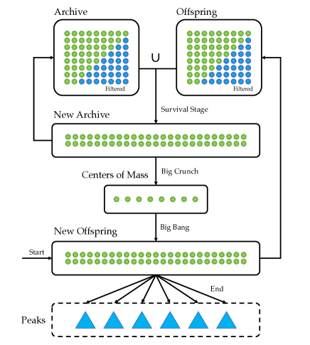
Figure 1: Basic framework of MGP-BBBC.

In this work, we propose a novel MMEA that adapts the Big Bang-Big Crunch algorithm (BBBC)[30] to solve MMOPs. We selected this algorithm based on its significantly better performance in single global optimization with respect to other classic EAs [31], and we propose to investigate its performances when extended to multimodal optimization. Our algorithm, namely the Multiple Global Peaks BBBC algorithm (MGP-BBBC), is a cluster-based method and a niching-based extension of the k-Cluster BBBC algorithm (k-BBBC)[22]. MGP-BBBC overcomes k-BBBC’s limitation of knowing the number of optima sought by using a nonparametric clustering method and aims at retrieving only the global peaks rather than the local as well. Besides a termination condition (often based on a maximum number of generations $g$) and the MMOP to be solved $f$, MGP-BBBC only features two user-defined parameters: the size of the population $n$ and the clustering bandwidth $h$.

Fig. 1 shows the basic framework of MGP-BBBC, in which each component brings a different contribution to solve the challenge of MMOPs. MGP-BBBC proposes: a survival stage that allows isolated individuals with worse fitness to win the environmental selection, such that small and sharp peaks are not missed; the big-crunch operator that reduces the population into different centers of mass and assigns them a number of desired offspring based on the niche count of their respective cluster, to increase the selection pressure of isolated individuals; and the big-bang operator that produces offspring by dynamically turning exploration into exploitation in the second half of the generation loop, targeting specific high levels of accuracy. We evaluated the performance of MGP-BBBC on the widely used CEC’2013 benchmark set containing twenty multimodal test functions. Compared with the state-of-the-art multimodal optimization algorithms, MGP-BBBC performs better than ten over thirteen algorithms and performs competitively against the other three.

The rest of the paper is organized as follows: Sec. 2 describes the original BBBC algorithm; Sec. 3 describes the proposed MGP-BBBC algorithm; Sec. 4 presents the experimental studies; and finally, Sec. 5 summarizes the work and presents possible future ideas.

2 Big Bang-Big Crunch Algorithm

The Big Bang-Big Crunch (BBBC) algorithm was proposed by Erol et al. [30, 32] to address some of the biggest disadvantages of genetic algorithms: premature convergence, convergence speed, and execution time. Inspired by the evolution of the universe, it is composed of two phases: (i) explosion, or big bang, in which the energy dissipation produces disorder and randomness, and (ii) implosion, or big crunch, in which randomness is drawn back into a different order. BBBC creates an initial random population $P$ uniformly spread throughout the search space (bang), evaluates its individuals, and groups them into their center of mass (crunch). These two phases are repeated, generating new solutions progressively closer to the center of mass. Finally, the center of mass converges to the optimal solution of the problem.

BBBC features different big-crunch operators [32] to calculate the center of mass $c$. The simplest way is choosing the most fitting individual as in Eqn. (1).

$$c=\begin{dcases}\textbf{x}_{j}:f(\textbf{x}_{j})=\max_{i=1}^{n}{f(\textbf{x}_{i})}\;\text{if max}\\ \textbf{x}_{j}:f(\textbf{x}_{j})=\min_{i=1}^{n}{f(\textbf{x}_{i})}\;\text{if min}\end{dcases},\;\textbf{x}_{i}\in P$$ (1)

The big-bang operator generates new individuals $\textbf{x}^{new}$ for the next population as expressed in Eqn. (2). The center of mass $c$ is disturbed with a random number $r$, which is multiplied by the search space upper bound $\textbf{x}^{U}$ (to ensure the newly generated individual being within the search space) and divided by the current iteration step $i$ (to progressively reduce the extent of the expansion in the search space and guaranteeing convergence). Note that the iteration step can also be multiplied by a further parameter to adjust the extent of expansion and quicken convergence [33] – a property that MGP-BBBC uses for exploitation as discussed in Sec. 3.3.

$$\textbf{x}^{new}=c+\frac{\textbf{x}^{U}r}{i},\quad\textbf{x}\in P$$ (2)

3 Multiple Global Peaks BBBC

Multiple Global Peaks BBBC (MGP-BBBC) is a multimodal extension of the BBBC algorithm (Sec. 1). Similar to its predecessor k-BBBC [22], MGP-BBBC identifies the multiple centers of mass by dividing the population into clusters. However, while k-BBBC relied on k-means [34] and therefore required a given-fixed number of clusters, MGP-BBBC is based on the mean-shift clustering [35, 36], which automatically determines the number of clusters by identifying dense regions in the dataset space. Furthermore, unlike k-BBBC, MGP-BBBC amis at localizing only the global peaks, disregarding any local sub-optimal solution.

input : Population size $n$, number of generations $g$, clustering bandwidth $h$, optimization problem $f$

output : Archive of elites $A$

1 begin

2       $O\leftarrow\textnormal{{randomInitialization}}(n)$;

3       $A\leftarrow\emptyset$;

4       $th\leftarrow h$;

5       for $it\leftarrow 1$ to $g$ do

6             if $it\neq 1$ then

7                   $O\leftarrow\textnormal{{bigBang}}(COM,it,g,OPC,f)$;

8                  

9            $O\leftarrow\textnormal{{evaluation}}(O,f)$;

10             $A,th\leftarrow\textnormal{{survival}}(O,A,th)$;

11             $COM,OPC\leftarrow\textnormal{{bigCrunch}}(A,h)$;

12            

13      return $A$;

14

Algorithm 1 MGP-BBBC

Algorithm 1 shows MGP-BBBC’s framework. The input parameters are the population size $n$, the maximum number of generations $g$ (which can also be replaced by a maximum number of function evaluations), the clustering bandwidth for the mean-shift clustering $h$ (defined in Sec. 3.2, which significantly affects the performance as detailed in Sec. 4.4), and the optimization problem $f$ (which includes the objective function, its dimensionality, search bounds, and constraints if any). The multiple global peaks are stored in an archive of elites $A$, separated from the rest of the population, which we will refer to as the population of offspring $O$. it initializes $O$ with $n$ randomly generated individuals within the problem’s bounds (line 2) and $A$ to an empty set (line 3); then, in the generational loop (lines 5-10), it evaluates $O$ (line 8, this procedure is reported in the supplementary material under Algorithm S.1), identifies elites to store in $A$ with a survival stage (line 9), crunches the elites to their centers of mass $C$ through clustering (line 10), and generates a new population from $C$ with a given number of offspring per each center of mass $OPC$ (line 7). The following subsection will describe each of these phases.

In MGP-BBBC, both $O$ and $A$ have the same size $n$. Each individual in the population is an object containing the values of the decision variables (attribute .x), the fitness (attribute .fit), and an additional boolean tag for removal from the population during filtering (attribute .tag, reported only in the supplementary material under Algorithm S.3).

input : Offspring population $O$, archive of elites $A$, filtering threshold $th$

output : New archive of elites $A$, updated filtering threshold $th$

1 begin

2       $n\leftarrow$ size of $O$;

3       if $A\neq\emptyset$ then

4             $D_{A}\leftarrow\textnormal{{pairwiseDistances}}(A)$;

5             $D_{O}\leftarrow\textnormal{{pairwiseDistances}}(O)$;

6             do

7                   $A^{\prime}\leftarrow\textnormal{{filtering}}(A,D_{A},th)$;

8                   $O^{\prime}\leftarrow\textnormal{{filtering}}(O,D_{O},th)$;

9                   $A\leftarrow O^{\prime}\cup A^{\prime}$;

10                   $n^{\prime}\leftarrow$ size of $A$;

11                   if $n^{\prime}<n$ then

12                         $th\leftarrow th\cdot 0.9$;

13                        

14                  

15            while $n^{\prime}<n$;

16            $\textnormal{{sort}}(A)$ by fitness;

17             resize $A$ by keeping the first $n$ individuals;

18            

19      else

20             $A\leftarrow O$;

21            

22      return $A,th$;

23

Algorithm 2 Survival Stage

input : Population $P$

output : Array of pairwise distances $D$ (having $\frac{n-1}{2}$ rows, each of them storing (1) pairwise distance, (2) index of first individual in $P$, and (3) index of second individual in $P$

1 begin

2       $n\leftarrow$ size of $P$;

3       $n\leftarrow n\cdot\frac{n-1}{2}$;

4       $D\leftarrow\emptyset$;

5       for $k\leftarrow 1$ to $n$ do

6             for $j\leftarrow i+1$ to $|n|$ do

7                   $d.\texttt{dist}\leftarrow\norm{P_{i},P_{j}}^{2}$;

8                   $d.\texttt{ind1}\leftarrow i$;

9                   $d.\texttt{ind2}\leftarrow j$;

10                   $D\leftarrow D\cup\{d\}$;

11                  

12            

13      return $D$;

14

Algorithm 3 Pairwise Distances

input : Population $P$, array of pairwise distances $D$, proximity threshold $th$

output : Filtered population $P^{\prime}$

1 begin

2       $P^{\prime}\leftarrow\emptyset$;

3       for $i\leftarrow 1$ to $|P|$ do

4             $P_{i}.\texttt{tag}\leftarrow 0$;

5            

6      for $k\leftarrow 1$ to $|D|$ do

7             if $D_{k}.\texttt{dist}<th$ then

8                   $i\leftarrow D_{k}.\texttt{ind1}$;

9                   $j\leftarrow D_{k}.\texttt{ind2}$;

10                   if $P_{i}.\texttt{tag}=0\wedge P_{j}.\texttt{tag}=0$ then

11                         /* for maximization problems */
if $P_{i}.\texttt{fit}\geq P_{j}.\texttt{fit}$ then

12                               $P_{j}.\texttt{tag}\leftarrow 1$;

13                              

14                        else

15                               $P_{i}.\texttt{tag}\leftarrow 1$;

16                              

17                        

18                  

19            

20      for $i\leftarrow 1$ to $|P|$ do

21             if $P_{i}.\texttt{tag}=0$ then

22                   $P^{\prime}\leftarrow P^{\prime}\cup\{P_{i}\}$;

23                  

24            

25      return $P^{\prime}$;

26

Algorithm 4 Filtering Operation

3.1 Survival Stage

Algorithm 2 shows the survival stage, which identifies the elites in the population and stores them in an archive $A$ having the same size as the population $O$. An elite is defined as an individual with high fitness, and MGP-BBBC filters out non-elites with a $\mu+\lambda$ schema [37] (lines 14-15). However, by doing so, two suboptimal individuals close to the same peak might filter out a third isolated suboptimal individual with worse fitness but close to another peak – therefore, missing that peak. This is even more exacerbated in problems featuring peaks with different sizes of concave regions, such as the Vincent function shown in Fig. 2(a). It is more likely that a uniform exploration of the search space would generate elites around the large peak rather than the small one.

Therefore, before non-elite removal, MGP-BBBC applies a distance-based filtering operation: it calculates all the pairwise distances in the population $A$ and $O$ (lines 4-5), and then applies the filtering procedure shown in Fig. 2(b) on both populations separately (lines 7-8). For each pair of individuals, this operation removes the one with worse fitness if their distance is smaller than a threshold $th$, allowing far away individuals to dominate over individuals in high-density regions. The pseudocode of the pairwise distances and the filtering operation are reported in Algorithm 3 and 4, respectively. The new archive of elites $A$ is then composed of the union of the filtered populations (line 9).

However, the size of the new archive $A$ must be greater or equal to the desired population size $n$ for the $\mu+\lambda$ schema to work. This might not always be the case, depending on the extent of filtering performed: the larger the threshold $th$, the more individuals will be filtered out. Therefore, MGP-BBBC dynamically tunes the value of the threshold starting from the same value as the clustering bandwidth $h$ (line 4 of Algorithm 1) and decreasing it by a small amount (i.e., by $10\%$) until the size of the archive is greater or equal to $n$ (lines 6-13). As the generations increase and the population converges to the peaks, the value of $th$ will also decrease.

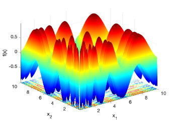
(a) Vincent with 2D

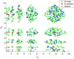
(b) Population Filtering

Figure 2: Distribution of elites (green and blue circles) around the global peaks (red crosses) for Vincent with 2D function ($F_{7}$ of CEC’2013 benchmark set). The plot shows that more elites tend to surround the prominent peaks (up-right area) due to the higher density of high fitness points rather than the smaller sharper ones (down-left area) – and many peaks in the down-left area are missed. The filtering procedure will remove points close to each other (blue circles), allowing MGP-BBBC to explore surroundings in low-density areas when producing new offspring.

Note that the first time MGP-BBBC calls the survival stage, $A$ will be empty (line 3) and, therefore, assigned directly to be filled with the individuals in the current population $O$ (lines 16-17). Furthermore, sorting (line 14) is based on the individuals’ fitness, and it is in descending or ascending order based on maximization or minimization problems, respectively.

With the time complexity of the pairwise distance calculation and filtering operation being both $\mathcal{O}(n^{2})$, the time complexity of the survival stage of MGP-BBBC is $\mathcal{O}(\delta_{th}\cdot n^{2}+n\log{n})$ – where the term $\delta_{th}$ indicates the number of decrements of $th$, which at most depends on its data type resolution until data underflow. If data underflow occurs, then the remainder in $A$ is filled with old elites randomly picked.

3.2 Big Crunch

Algorithm 5 shows the big-crunch operator of MGP-BBBC, which identifies the centers of mass $COM$ within the archive $A$. This operation relies on mean-shift clustering [35, 36], which iteratively shifts each point to a higher-density position until convergence. The points converging to the same position are assigned to the same cluster. The procedure is reported in the supplementary material under Algorithm S.2, and it uses a flat kernel function requiring a bandwidth parameter $h$. The kernel bandwidth defines the neighborhood size for density estimation, influencing how points are grouped into clusters: a smaller bandwidth results in more compact clusters, while a larger one creates broader clusters. However, the bandwidth’s impact on clustering is influenced by data density rather than directly by the space’s size, making it crucial to choose a bandwidth suited to the dataset’s scale for meaningful results (see Sec. 4.4). Due to the bandwidth’s geometrical role, MGP-BBBC uses its value $h$ to initialize the threshold $th$ of the filtering in the survival stage (see Sec. 3.1).

Once the big-bang operator retrieves a set of clusters $C$ (line 2), it identifies the individual with the best fitness for each cluster (lines 6-9), which is added into the set $COM$ (line 10). Lastly, the big-bang operator defines the number of desired offspring that will be generated for each center of mass: ultimately, the overall number of offspring must be equal to $n$; however, the number of clusters (and thus, centers of mass) retrieved by the mean-shift clustering varies based on the input dataset. In early generations, it is likely that the big-bang operator will retrieve many centers of mass, whereas in late generations, there will be fewer. Therefore, MGP-BBBC assigns a desired number of offspring per center of mass $OPC$ (which total sums up to $n$) based on the niche count $NC$ for each cluster, stored at line 11. Specifically, it assigns more offspring to centers of mass having a niche count smaller than the average of $NC$, to promote isolated individuals and prevent high-density regions from being overcrowded. The procedure is reported in Algorithm 6 and executed at line 12.

With the time complexity of the mean-shift clustering being $\mathcal{O}(n^{2})$ (the number of iterations for convergence is not an input, and the bandwidth $h$ influences the algorithm’s behavior but does not change the fundamental complexity), a number of clusters that is upper bounded by $n$ and therefore $\mathcal{O}(n)$ for both finding the best individual for each cluster and calculating $OPC$, the time complexity of the big-crunch operator of MGP-BBBC is dominated by the clustering: $\mathcal{O}(n^{2})$.

input : Archive $A$, clustering bandwidth $h$

output : Array of centers of mass $COM$, array containing number of desired offspring per each center of mass $OPC$

1 begin

2       $C\leftarrow\textnormal{{meanShiftClustering}}(A.\texttt{x},h)$;

3       $COM\leftarrow\emptyset$;

4       $NC\leftarrow\emptyset$;

5       for $i\leftarrow 1$ to $|C|$ do

6             $c_{\text{best}}\leftarrow(C_{i_{1}})$;

7             for $c_{j}\in C_{i}$ do

8                   /* for maximization problems */
if $c_{\text{best}}.\texttt{fit}<c_{j}.\texttt{fit}$ then

9                         $c_{\text{best}}\leftarrow c_{j}$;

10                        

11                  

12            

13            $COM\leftarrow COM\cup\{c_{\text{best}}\}$;

14             $NC\leftarrow NC\cup\{|C_{i}|\}$;

15            

16      $OPC\leftarrow\textnormal{{offspringPerCOM}}(|A|,NC)$;

17       return $COM,OPC$;

18

Algorithm 5 Big Crunch

input : Size of desired offspring population $n$, niche count per center of mass $NC$

output : Array containing number of desired offspring per each center of mass $OPC$

1 begin

2       $OPC\leftarrow\emptyset$;

3       $avg\leftarrow\textnormal{{mean}}(NC)$;

4       for $i\leftarrow 1$ to $|NC|$ do

5             $OPC_{i}\leftarrow\textnormal{{round}}(avg)$;

6            

7      $n^{\prime}\leftarrow\textnormal{{sum}}(OPC)$;

8       if $n^{\prime}<n$ then

9             for $i\leftarrow 1$ to $\textnormal{{mod}}(n,n^{\prime})$ do

10                   do

11                         $j\leftarrow\textnormal{{randi}}(1,|NC|)$;

12                        

13                  while $NC_{j}>\textnormal{{floor(}}\textnormal{\emph{avg}}\textnormal{{)}}$;

14                  $OPC_{j}\leftarrow OPC_{j}+1$;

15                  

16            

17      else if $n^{\prime}>n$ then

18             for $i\leftarrow 1$ to $n^{\prime}-n$ do

19                   do

20                         $j\leftarrow\textnormal{{randi}}(1,|NC|)$;

21                        

22                  while $NC_{j}<\textnormal{{floor(}}\textnormal{\emph{avg}}\textnormal{{)}}$;

23                  $OPC_{j}\leftarrow OPC_{j}-1$;

24                  

25            

26      return $OPC$;

27

Algorithm 6 Offspring per Center of Mass

input : Array of centers of mass $COM$, generation number $it$, max number of generations $g$, array containing the number of desired offspring per each center of mass $OPC$, optimization problem $f$

output : Offspring population $O$

1 begin

2       $O\leftarrow\emptyset$;

3       $e\leftarrow\textnormal{{getExtent}}(it,g,f)$;

4       for $i\leftarrow 1$ to $|COM|$ do

5             for $j\leftarrow 1$ to $OPC_{i}$ do

6                   $X\leftarrow COM_{i}.\texttt{x}+e\cdot\textnormal{{rand}}(-1,1)$;

7                   $X\leftarrow\textnormal{{min}}(\textnormal{{max}}(X,f.\texttt{lowB}),f.\texttt{uppB})$;

8                  

9                  $O\leftarrow O\cup\{X\}$;

10                  

11            

12      

13      return $O$;

14

Algorithm 7 Big Bang

input : Current iteration counter $it$, max number of generations $g$, optimization problem $f$

output : Extent of expansion $e$

1 begin

2       if $it<g\cdot 0.6$ then

3             $e_{1}\leftarrow\frac{f.\texttt{uppB}-f.\texttt{lowB}}{4}$;

4             $a\leftarrow\frac{e_{1}-1.0\cdot 10^{-1}}{\log\left(g\cdot 0.6\right)}$;

5             $e\leftarrow e_{1}-a\cdot\log\left(it+1\right)$;

6            

7      else

8             $I\leftarrow\left\{1.0\cdot 10^{-1},1.0\cdot 10^{-2},1.0\cdot 10^{-3},1.0\cdot 10^{-4},1.0\cdot 10^{-5}\right\}$;

9             $z\leftarrow\textnormal{{floor}}(\frac{g-it}{5})$;

10             for $i\leftarrow 1$ to $5$ do

11                   if $z\cdot(i-1)\leq it\wedge it<z\cdot i$ then

12                         $e\leftarrow I_{i}$;

13                        

14                  

15            

16      return $e$;

17

Algorithm 8 Get Bang Extent of Expansion

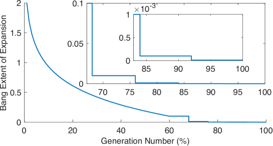
Figure 3: Reduction of the bang extent of expansion over generations. In the example, the extent starts from $2.0$ and decreases logarithmically until the $60\%$ of the total number of generations (exploration phase) when it reaches a value of $1.0E-01$. After that, it decreases with constant steps to target the other levels of accuracy ($1.0E-02$, $1.0E-03$, $1.0E-04$, and $1.0E-05$) in an equal number of generations (exploitation phase). Zoomed-in plots allow readers to appreciate the details of the exploitation phase.

3.3 Big Bang

Algorithm 7 shows the big-bang operator of MGP-BBBC, which generates new offspring $O$ from the centers of mass $COM$ retrieved by the big-crunch operator (see Sec. 5). While generating offspring, it is essential to properly balance exploration and exploitation to retrieve peaks with high accuracy. To achieve this balance, MGP-BBBC dynamically tunes the extent of expansion of the big-bang operator (line 2). While the standard BBBC algorithm decrements the extent linearly as specified in Eqn. (2), MGP-BBBC divides it into two trends based on the total number of generations $g$ – as shown in Fig. 3. During the first $60\%$ of generations, the extent is decreased logarithmically from a starting value (empirically set to be one-fourth of the problem’s bound when it was observed a population distributed on the search rather than on the bounds) to $1.0E-01$: in this phase, MGP-BBBC will explore the surroundings of the centers of mass, localizing as many global peaks as possible. During the last $40\%$ of generations, the extent will follow a constant trend with five uniformly distributed steps, going from $1.0E-01$ to $1.0E-05$: in this phase, MGP-BBBC will exploit the centers of mass, converging with high accuracy to the respective global peak. The pseudocode of the procedure is reported in Algorithm 8.

Once the extent of expansion $e$ is set for its current iteration, the big-bang operator applies it on every center of mass (line 4), producing a number of offspring defined by the respective element in $OPC$ (line 5). Each offspring is produced by applying a random disturbance with, at most, a magnitude equal to $e$ (lines 6-8). Note that the new individual $X$ is generated within the bounds of the search space with the filtering formula at line 7, which is applied to all decision variables and their respective bounds.

With the time complexity of calculating the extent being constant, the complexity of the big-bang operator is only determined linearly by the amount of offspring to be produced: $\mathcal{O}(nd)$, where $d$ is the dimensionality of the MMOP.

4 Experimental Study

Table 1: Properties of the twenty multimodal test functions in the CEC’2013 benchmark set

Function	Name	Dimension Size	No. of Global Optima	No. of Local Optima	Max Function Evaluations
$F_{1}$	Five-Uneven-Peak Trap	1	2	3	${5.0}\mathrm{E}{+04}$
$F_{2}$	Equal Maxima	1	5	0	${5.0}\mathrm{E}{+04}$
$F_{3}$	Uneven Decreasing Maxima	1	1	4	${5.0}\mathrm{E}{+04}$
$F_{4}$	Himmelblau	2	4	0	${5.0}\mathrm{E}{+04}$
$F_{5}$	Six-Hump Camel Back	2	2	2	${5.0}\mathrm{E}{+04}$
$F_{6}$	Shubert with 2D	2	18	many	${2.0}\mathrm{E}{+05}$
$F_{7}$	Vincent with 2D	2	36	0	${2.0}\mathrm{E}{+05}$
$F_{8}$	Shubert with 3D	3	81	many	${4.0}\mathrm{E}{+05}$
$F_{9}$	Vincent with 3D	3	216	0	${4.0}\mathrm{E}{+05}$
$F_{10}$	Modified Rastrigin	2	12	0	${2.0}\mathrm{E}{+05}$
$F_{11}$	Composition Function 1 with 2D	2	6	many	${2.0}\mathrm{E}{+05}$
$F_{12}$	Composition Function 2 with 2D	2	8	many	${2.0}\mathrm{E}{+05}$
$F_{13}$	Composition Function 3 with 2D	2	6	many	${2.0}\mathrm{E}{+05}$
$F_{14}$	Composition Function 3 with 3D	3	6	many	${4.0}\mathrm{E}{+05}$
$F_{15}$	Composition Function 4 with 3D	3	8	many	${4.0}\mathrm{E}{+05}$
$F_{16}$	Composition Function 3 with 5D	5	6	many	${4.0}\mathrm{E}{+05}$
$F_{17}$	Composition Function 4 with 5D	5	8	many	${4.0}\mathrm{E}{+05}$
$F_{18}$	Composition Function 3 with 10D	10	6	many	${4.0}\mathrm{E}{+05}$
$F_{19}$	Composition Function 4 with 10D	10	8	many	${4.0}\mathrm{E}{+05}$
$F_{20}$	Composition Function 4 with 20D	20	8	many	${4.0}\mathrm{E}{+05}$

4.1 Benchmark Functions and Performance Metrics

We used the CEC’2013 benchmark set [38] to evaluate MGP-BBBC performances. The CEC’2013 benchmark set contains twenty multimodal maximization problems, listed in Table 1 with their properties. Specifically, $F_{1}-F_{3}$ are simple mono-dimensional functions, $F_{4}-F_{7}$ and $F_{10}$ are scalable two-dimensional functions, $F_{8}-F_{9}$ are scalable three-dimensional functions, and $F_{11}-F_{20}$ are complex composition functions with dimensionality ranging from two to twenty.

We executed each problem by setting a maximum number of function evaluations (MaxFEs) based on the procedure established in the literature [38], which we report in the rightmost column of Table 1. MaxFEs sets the total number of runs (NR) for each problem, given the population size. Based on this, we evaluated the algorithm’s performance with the following two metrics:

• peak ratio (PR), the average percentage of global peaks found over multiple runs, defined in Eqn. (3) as the sum of the number of global peaks for each run (NPF) divided by the total number of global peaks (TPN) times the total number of runs (NR); and

  $$\text{PR}=\frac{\sum^{\text{NR}}_{i=1}{\text{NPF}_{i}}}{\text{TNP}\cdot\text{NR}}$$ (3)

• success ratio (SR), the percentage of successful runs among multiple runs (i.e., runs that correctly retrieved all global optima), defined in Eqn. (4) as the ratio between the number of successful (NSR) and the total number of runs (NR).

  $$\text{SR}=\frac{\text{NSR}}{\text{NR}}$$ (4)

Table 2: MGP-BBBC Best Parameter Settings

Func.	Pop. Size ($n$)	$h$		Func.	Pop. Size ($n$)	$h$
$F_{1}$	1000	0.80		$F_{11}$	1000	0.40
$F_{2}$	1000	0.08		$F_{12}$	1000	0.60
$F_{3}$	1000	0.80		$F_{13}$	1000	0.40
$F_{4}$	1000	0.80		$F_{14}$	1000	1.40
$F_{5}$	1000	0.80		$F_{15}$	500	2.00
$F_{6}$	1000	0.20		$F_{16}$	1000	3.60
$F_{7}$	500	0.20		$F_{17}$	500	4.00
$F_{8}$	1000	0.60		$F_{18}$	500	4.00
$F_{9}$	1000	0.40		$F_{19}$	500	6.00
$F_{10}$	1000	0.40		$F_{20}$	500	10.00

Lastly, we analyzed the results based on three accuracy levels: $\varepsilon={1.0}\mathrm{E}{-03}$, $\varepsilon={1.0}\mathrm{E}{-04}$, and $\varepsilon={1.0}\mathrm{E}{-05}$. Based on the procedure established in the literature [39, 5], we mainly discuss the results with accuracy $\varepsilon={1.0}\mathrm{E}{-04}$, whereas the results with other levels are reported in the supplementary material.

4.2 Compared Algorithms and Parameter Configurations

We compared MGP-BBBC with its base version k-BBBC [22] and twelve other MMOEAs from the state-of-the-art: SSGA [27], SDE-GA, RSCMSA [28], RLSIS, HillVallEA [29], FastNichingEP, EMSO-MMO, CMSA-ES-DIPS, ANBNWI-DE, DIDE [26], MOMMOP [40], and EMO-MMO [41] – most of these algorithms participated to competitions in either CEC or GECCO throughout 2017 and 2020 (the latest at the time of this work). The settings of MGP-BBBC were set accordingly to Sec. 4.4 and reported on Table 2, whereas the results of the state-of-the-art algorithms were collected from the CEC repository or according to their corresponding references.

We ran fifty independent runs (NR$=50$) and averaged the results for a fair comparison. We used the Wilcoxon rank-sum test [42] to statistically evaluate the results, with significance level $\alpha=0.05$. In the tables reporting the results, we added a $+$ sign to identify when MGP-BBBC is significantly better, a $-$ sign when it is significantly worse, and a $\approx$ sign when results are not significantly different.

Table 3: Experimental results of peak ratio and success rate on the CEC’2013 benchmark set at the accuracy level $\varepsilon=1.0E-04$

Func.	MGP-BBBC		k-BBBC		SSGA		SDE-GA		RSCMSA		RLSIS		HillVallEA
	PR	SR	PR	SR	PR	SR	PR	SR	PR	SR	PR	SR	PR	SR
$F_{1}$	1.000	1.000	1.000($\approx$)	1.000	1.000($\approx$)	1.000	1.000($\approx$)	1.000	1.000($\approx$)	1.000	1.000($\approx$)	1.000	1.000($\approx$)	1.000
$F_{2}$	1.000	1.000	1.000($\approx$)	1.000	1.000($\approx$)	1.000	1.000($\approx$)	1.000	1.000($\approx$)	1.000	1.000($\approx$)	1.000	1.000($\approx$)	1.000
$F_{3}$	1.000	1.000	1.000($\approx$)	1.000	1.000($\approx$)	1.000	1.000($\approx$)	1.000	1.000($\approx$)	1.000	1.000($\approx$)	1.000	1.000($\approx$)	1.000
$F_{4}$	1.000	1.000	1.000($\approx$)	1.000	0.155($+$)	0.000	1.000($\approx$)	1.000	0.995($\approx$)	0.980	1.000($\approx$)	1.000	1.000($\approx$)	1.000
$F_{5}$	1.000	1.000	1.000($\approx$)	1.000	0.460($+$)	0.200	1.000($\approx$)	1.000	0.980($\approx$)	0.960	1.000($\approx$)	1.000	1.000($\approx$)	1.000
$F_{6}$	1.000	1.000	0.943($+$)	0.280	1.000($\approx$)	1.000	1.000($\approx$)	1.000	0.999($\approx$)	0.980	0.872($+$)	0.100	1.000($\approx$)	1.000
$F_{7}$	0.998	0.920	0.744($+$)	0.000	0.901($+$)	0.000	1.000($-$)	1.000	0.962($+$)	0.280	0.920($+$)	0.000	1.000($-$)	1.000
$F_{8}$	1.000	1.000	0.000($+$)	0.000	1.000($\approx$)	1.000	1.000($\approx$)	1.000	0.871($+$)	0.000	0.189($+$)	0.000	0.920($+$)	0.000
$F_{9}$	0.477	0.000	0.005($+$)	0.000	0.518($-$)	0.000	0.986($-$)	0.020	0.627($-$)	0.000	0.584($-$)	0.000	0.945($-$)	0.000
$F_{10}$	1.000	1.000	1.000($\approx$)	1.000	1.000($\approx$)	1.000	1.000($\approx$)	1.000	1.000($\approx$)	1.000	1.000($\approx$)	1.000	1.000($\approx$)	1.000
$F_{11}$	1.000	1.000	1.000($\approx$)	1.000	1.000($\approx$)	1.000	1.000($\approx$)	1.000	0.997($\approx$)	0.980	1.000($\approx$)	1.000	1.000($\approx$)	1.000
$F_{12}$	1.000	1.000	0.920($+$)	0.360	1.000($\approx$)	1.000	1.000($\approx$)	1.000	0.948($+$)	0.580	0.988($+$)	0.900	1.000($\approx$)	1.000
$F_{13}$	1.000	1.000	0.993($\approx$)	0.960	0.957($+$)	0.760	0.920($+$)	0.520	0.997($\approx$)	0.980	0.993($\approx$)	0.960	1.000($\approx$)	1.000
$F_{14}$	0.930	0.580	0.857($+$)	0.140	0.727($+$)	0.020	0.670($+$)	0.000	0.810($+$)	0.060	0.833($+$)	0.140	0.917($\approx$)	0.560
$F_{15}$	0.718	0.000	0.658($+$)	0.000	0.563($+$)	0.000	0.750($-$)	0.000	0.748($-$)	0.000	0.798($-$)	0.200	0.750($-$)	0.000
$F_{16}$	0.707	0.000	0.710($\approx$)	0.000	0.673($+$)	0.000	0.667($+$)	0.000	0.667($+$)	0.000	0.677($+$)	0.000	0.687($\approx$)	0.000
$F_{17}$	0.598	0.000	0.543($+$)	0.000	0.485($+$)	0.000	0.703($-$)	0.000	0.703($-$)	0.000	0.845($-$)	0.280	0.750($-$)	0.000
$F_{18}$	0.663	0.000	0.440($+$)	0.000	0.307($+$)	0.000	0.667($\approx$)	0.000	0.667($\approx$)	0.000	0.667($\approx$)	0.000	0.667($\approx$)	0.000
$F_{19}$	0.355	0.000	0.375($\approx$)	0.000	0.023($+$)	0.000	0.555($-$)	0.000	0.503($-$)	0.000	0.610($-$)	0.040	0.585($-$)	0.000
$F_{20}$	0.358	0.000	0.000($+$)	0.000	0.000($+$)	0.000	0.455($-$)	0.000	0.483($-$)	0.000	0.423($-$)	0.000	0.483($-$)	0.000
Total $+$ (Significantly better)			10		11		3		5		6		1
Total $\approx$ (Not sig. different)			10		8		11		10		9		13
Total $-$ (Significantly worse)			0		1		6		5		5		6
Func.	FastNichingEP		EMSO-MMO		CMSA-ES-DIPS		ANBNWI-DE		DIDE		MOMMOP		EMO-MMO
	PR	SR	PR	SR	PR	SR	PR	SR	PR	SR	PR	SR	PR	SR
$F_{1}$	0.910($+$)	0.820	1.000($\approx$)	1.000	1.000($\approx$)	1.000	1.000($\approx$)	1.000	1.000($\approx$)	1.000	1.000($\approx$)	1.000	1.000($\approx$)	1.000
$F_{2}$	1.000($\approx$)	1.000	1.000($\approx$)	1.000	1.000($\approx$)	1.000	0.988($\approx$)	0.940	1.000($\approx$)	1.000	1.000($\approx$)	1.000	1.000($\approx$)	1.000
$F_{3}$	1.000($\approx$)	1.000	1.000($\approx$)	1.000	1.000($\approx$)	1.000	1.000($\approx$)	1.000	1.000($\approx$)	1.000	1.000($\approx$)	1.000	1.000($\approx$)	1.000
$F_{4}$	0.975($+$)	0.900	0.990($\approx$)	0.960	0.700($+$)	0.180	0.990($\approx$)	0.960	1.000($\approx$)	1.000	0.985($+$)	0.940	1.000($\approx$)	1.000
$F_{5}$	1.000($\approx$)	1.000	1.000($\approx$)	1.000	0.440($+$)	0.200	1.000($\approx$)	1.000	1.000($\approx$)	1.000	1.000($\approx$)	1.000	1.000($\approx$)	1.000
$F_{6}$	0.496($+$)	0.000	1.000($\approx$)	1.000	1.000($\approx$)	1.000	1.000($\approx$)	1.000	1.000($\approx$)	1.000	1.000($\approx$)	1.000	1.000($\approx$)	1.000
$F_{7}$	0.516($+$)	0.000	0.970($+$)	0.740	0.539($+$)	0.000	0.946($+$)	0.140	0.921($+$)	0.040	1.000($-$)	1.000	1.000($-$)	1.000
$F_{8}$	0.259($+$)	0.000	0.988($+$)	0.720	0.594($+$)	0.000	0.924($+$)	0.000	0.692($+$)	0.000	1.000($\approx$)	1.000	1.000($\approx$)	1.000
$F_{9}$	0.013($+$)	0.000	0.546($-$)	0.000	0.184($+$)	0.000	0.644($-$)	0.000	0.571($-$)	0.000	1.000($-$)	0.920	0.950($-$)	0.000
$F_{10}$	1.000($\approx$)	1.000	1.000($\approx$)	1.000	1.000($\approx$)	1.000	0.998($\approx$)	0.980	1.000($\approx$)	1.000	1.000($\approx$)	1.000	1.000($\approx$)	1.000
$F_{11}$	0.673($+$)	0.000	0.907($+$)	0.500	0.967($+$)	0.820	0.990($\approx$)	0.940	1.000($\approx$)	1.000	0.710($+$)	0.040	1.000($\approx$)	1.000
$F_{12}$	0.740($+$)	0.000	0.988($+$)	0.920	0.995($\approx$)	0.960	0.923($+$)	0.380	1.000($\approx$)	1.000	0.955($+$)	0.660	1.000($\approx$)	1.000
$F_{13}$	0.710($+$)	0.040	0.810($+$)	0.300	0.980($+$)	0.880	1.000($\approx$)	1.000	0.987($+$)	0.920	0.667($+$)	0.000	0.997($+$)	0.980
$F_{14}$	0.627($+$)	0.000	0.563($+$)	0.000	0.820($+$)	0.160	0.890($+$)	0.340	0.773($+$)	0.020	0.667($+$)	0.000	0.733($+$)	0.060
$F_{15}$	0.160($+$)	0.000	0.460($+$)	0.000	0.665($+$)	0.000	0.738($-$)	0.000	0.748($-$)	0.000	0.618($+$)	0.000	0.595($+$)	0.000
$F_{16}$	0.537($+$)	0.000	0.343($+$)	0.000	0.573($+$)	0.000	0.690($\approx$)	0.000	0.667($+$)	0.000	0.630($+$)	0.000	0.657($+$)	0.000
$F_{17}$	0.135($+$)	0.000	0.210($+$)	0.000	0.625($\approx$)	0.000	0.665($-$)	0.000	0.593($+$)	0.000	0.505($+$)	0.000	0.335($+$)	0.000
$F_{18}$	0.113($+$)	0.000	0.163($+$)	0.000	0.607($+$)	0.000	0.667($\approx$)	0.000	0.667($\approx$)	0.000	0.497($+$)	0.000	0.327($+$)	0.000
$F_{19}$	0.013($+$)	0.000	0.208($+$)	0.000	0.525($-$)	0.000	0.550($-$)	0.000	0.543($-$)	0.000	0.230($+$)	0.000	0.135($+$)	0.000
$F_{20}$	0.000($+$)	0.000	0.108($+$)	0.000	0.440($-$)	0.000	0.240($+$)	0.000	0.355($+$)	0.000	0.125($+$)	0.000	0.080($+$)	0.000
$+$	16		12		11		5		7		11		8
$\approx$	4		7		7		11		10		7		10
$-$	0		1		2		4		3		2		2

4.3 Comparison With State-of-the-Art Algorithms

Table 3 reports the experimental results of PR and SR on the CEC’2013 benchmark set with accuracy level $\varepsilon={1.0}\mathrm{E}{-04}$. The values are the best retrieved by MGP-BBBC and the other state-of-the-art algorithms – best PR and SR for each function are bolded. MGP-BBBC performed the best on twelve out of twenty functions, non-significantly different than the algorithms retrieving the best for two functions, and competitively on the other six functions.

MGP-BBBC features a performance of both PF and SR $=1.000$ in the functions $F_{1}-F_{6}$, $F_{8}$, $F_{10}-F_{13}$ – no other algorithm performs a perfect PR and SR past this point. The performance on $F_{7}$ (Vincent 2D), which features a sine function with a decreasing frequency, is also high: MGP-BBBC features the highest PR ($0.998$) and SR ($0.920$) among nine over thirteen algorithms, except for SDE-GA, HillVallEA, MOMMOP, and EMO-MMO (SR=$1.000$). In its three-dimensional counterpart $F_{9}$ (Vincent 3D), however, MGP-BBBC features a lower PR ($0.477$) than most of the other algorithms – this is possibly due to the high number of global peaks ($216$) and the respective MGP-BBBC’s requirement of a large population because of its cluster-based nature. Remarkably, MGP-BBBC features the best PR $=0.930$ among every algorithm on $F_{14}$ (a 3D composite function), competing only with HillVallEA, which features a not significantly lower PR. In the low-dimensionality composite functions $F_{15}$ (3D) and $F_{17}$ (5D), MGP-BBBC features a PR $=0.718$ and $=0.598$, respectively; both significantly worse than five algorithms out of thirteen: SDE-GA ($0.750$ and $0.703$), RSCMSA ($0.748$ and $0.703$), RLSIS ($0.798$ and $0.845$), HillVallEA ($0.750$ and $0.750$), and ANBNWI-DE ($0.738$ and $0.665$). However, in the 5D composite function $F_{16}$, MGP-BBBC features the second highest (non-significant) PR $=0.707$ against the best $0.710$ of k-BBBC, showing that BBBC algorithm is the best strategy for this function. In the 10D composite functions $F_{18}-F_{19}$, MGP-BBBC performs inconsistently: it ranks non-significantly different than the bests on $F_{18}$ with PR $=0.663$ on a par with SDE-GA, RSCMSA, RLSIS, and HillVallEA (demonstrating MGP-BBBC’s ability to handle high dimensionality); however, it ranks far from the best algorithms on $F_{19}$ with PR $=0.355$ against RLSIS ($0.610$) or HillVallEA ($0.585$). Lastly, on the 20D function $F_{20}$, MGP-BBBC features a PR value of $0.358$, not too far from the best $0.483$ of RSCMSA and HillVallEA – still outperforming eight over thirteen algorithms on this high-dimensional function.

At the bottom of each column, we reported the numbers of functions for which MGP-BBBC performed significantly better ($+$), worse ($-$), or not significantly different ($\approx$) according to the Wilcoxon rank-sum test. These numbers show that, in terms of PR, MGP-BBBC performs competitively compared to all the algorithms (i.e., the number of $+$ and $\approx$ is higher than the number of $-$) and performs better than ten out of thirteen algorithms (i.e., the number of $+$ is higher than the number of $-$), with only SDE-GA and HillVallEA outperforming it and with RSCMSA having same performances. Specifically, there are five out of thirteen cases in which the number of $+$ is higher than the sum of $-$ and $\approx$ (SSGA, FastNichingEP, EMSO-MMO, CMSA-ES-DIPS, and MOMMOP).

The experimental results for the accuracy levels $\varepsilon={1.0}\mathrm{E}{-03}$ and $\varepsilon={1.0}\mathrm{E}{-05}$ can be found in the supplementary material (Table S.I and S.II, respectively), further validating the competitive performance of MGP-BBBC.

4.4 Parameter Analysis

MGP-BBBC features two user-defined parameters: the population size $n$ (same value for both offspring and archive) and the clustering kernel bandwidth $h$ (see Sec. 3.2). While the first one is a common parameter of EAs, the second is specific to the clustering algorithm and depends on the optimization problem (i.e., bounds, landscape, number of optima).

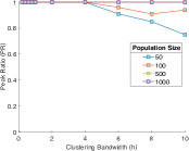
(a) $F_{1}$

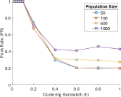
(b) $F_{2}$

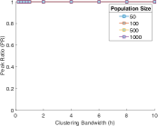
(c) $F_{3}$

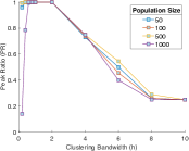
(d) $F_{4}$

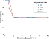
(e) $F_{5}$

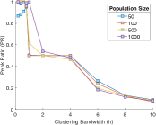
(f) $F_{6}$

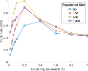
(g) $F_{7}$

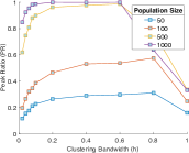
(h) $F_{8}$

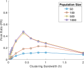
(i) $F_{9}$

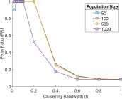
(j) $F_{10}$

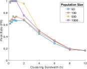
(k) $F_{11}$

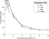
(l) $F_{12}$

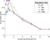
(m) $F_{13}$

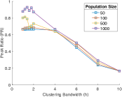
(n) $F_{14}$

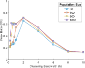
(o) $F_{15}$

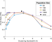
(p) $F_{16}$

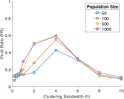
(q) $F_{17}$

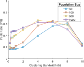
(r) $F_{18}$

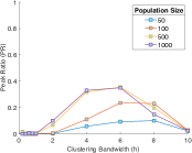
(s) $F_{19}$

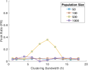
(t) $F_{20}$

Figure 4: Changes in the PR values (at the accuracy level $\varepsilon=1.0E-04$) with different Population Size (n) and Clustering Bandwith (h) on CEC’2013 benchmark set.

In terms of space geometry, the kernel bandwidth defines the radius of a sphere (in a multidimensional space) within which points are considered neighbors. The choice of kernel bandwidth significantly impacts the clustering result. Smaller bandwidths lead to tighter, more compact clusters and can result in more clusters, as points need to be closer to each other to be considered part of the same cluster. This makes clustering more sensitive to noise and outliers, as small changes in position can lead to different cluster assignments. On the other hand, larger bandwidths lead to more diffuse clusters, with the risk of merging two nearby clusters into a single cluster. However, this makes the clustering more robust to noise and outliers, as points farther apart can still be grouped together. Unfortunately, the relationship between kernel bandwidth and the size of the space is not linear. While the choice of bandwidth can be influenced by the scale of the data or the density of points, it is not directly proportional to the size of the space. Instead, it is related to the density of points and the desired level of granularity in the clustering result. This makes it essential to choose a bandwidth that is appropriate for the scale of the features in the dataset to achieve meaningful clustering results and requires us to select a proper value for each problem.

For a comprehensive parameter analysis, we first ran a preliminary study to observe which values to test on a large scale for both parameters. We observed that population sizes larger than 1000 individuals significantly reduce the performance of MGP-BBBC, except for problem $F_{17}$; however, this large number did not allow us to perform a full experiment due to high computational time: we set the tests for the population size to $n\in\{50,100,500,1000\}$. For the kernel bandwidth, we observed different ranges for different problems: the first thirteen problems of CEC’2013 required small bandwidth $h<1.0$, whereas the more complex composite functions required a large bandwidth $h<18.00$ – however, we clarify that we did not observe any strong correlation between the bandwidth $h$ and the search space (in terms of bounds, area, and diagonal of the search space) that would allow us to set a unique range of bandwidth for all problems. Once selected the range for each parameter, we choose a $4\times 10$ set of combinations (i.e., four values for $n$ and ten for $h$).

To observe how the values of these parameters affect the results of MGP-BBBC, we compared the best result for each function against each combination with the Wilcoxon rank-sum test at the significance level $\alpha=0.05$ (results are reported in the supplementary material under Tables S.III and S.IV for accuracy $\varepsilon=1.0E-03$, S.V and S.VI for $\varepsilon=1.0E-04$, and S.VII and S.VIII for $\varepsilon=1.0E-05$). The tables indicate the number of settings that performed significantly worse ($-$) or non-significantly different ($\approx$) than the best setting in terms of both population size (rows) and bandwidth (columns). The trend for each problem is graphically depicted in the supplementary material under Fig. S.1, S.2, and S.3 for accuracy $\varepsilon=1.0E-04$ only.

Lastly, we adopted Friedman’s test with the Bonferroni-Dunn procedure [42] to test the robustness of MGP-BBBC. Since the selected values of $h$ differ from problem to problem, Friedman’s test can analyze the results for solving each problem separately; however, since the population size was set to be the same for all problems, we ran the Friedman’s test to analyze the effect of the population size on all twenty problems as well. Table 4 shows the results of the population size among all the problems, whereas Tables from S.IX to S.XXVIII of the supplementary material show the results of both population size and bandwidth for each problem. The p-value shows the result of the Bonferroni-Dunn procedure; “Y” indicates that there is a significant difference (at the significance level $\alpha=0.05$) between the corresponding pairwise settings, whereas “N” indicates no significant difference.

The results show that MGP-BBBC’s performance improves as the population size increases; however, there are no significant differences between $n=500$ and $n=1000$ overall. Beyond this point, it is not worth investigating – although there might be some good results for $n=800$. Fig. 4 also show similar trends for $n=500$ and $n=1000$, with the only exception of $F_{20}$. In this problem, $n=500$ is the only setting that provided results, whereas the other population sizes show flat low trends; however, according to the Bonferroni-Dunn procedure (Tab. S.XXVIII), there is no statistical difference between $n=500$ and $n=1000$ for $F_{20}$ – this is possibly due to the large observation range of $h\in[2.0,18.0]$.

Table 4: Experimental results of Friedman Test with Bonferroni-Dunn Procedure on Population Size ($n$) over all the functions of CEC’2013

pair		1.00E-03		pair		1.00E-04		pair		1.00E-05
n1	n2	p-value	$\alpha=0.05$	n1	n2	p-value	$\alpha=0.05$	n1	n2	p-value	$\alpha=0.05$
50.00	100.00	0.003596	Y	50.00	100.00	0.002889	Y	50.00	100.00	0.001775	Y
50.00	500.00	1.70E-23	Y	50.00	500.00	6.78E-22	Y	50.00	500.00	1.71E-20	Y
50.00	1000.00	2.74E-25	Y	50.00	1000.00	2.18E-22	Y	50.00	1000.00	3.97E-20	Y
100.00	500.00	9.94E-11	Y	100.00	500.00	1.69E-09	Y	100.00	500.00	2.96E-08	Y
100.00	1000.00	6.11E-12	Y	100.00	1000.00	8.04E-10	Y	100.00	1000.00	5.03E-08	Y
500.00	1000.00	1	N	500.00	1000.00	1	N	500.00	1000.00	1	N
Not Significantly Different		1		Not Significantly Different		1		Not Significantly Different		1
Significantly Different		5		Significantly Different		5		Significantly Different		5

Regarding the clustering kernel bandwidth $h$, there is no significant impact on the performance of the problems $F_{1}-F_{5}$, $F_{10}$, and $F_{19}-F_{20}$, whereas for the other problems observe significant distance. From the trends shown in Fig. 4, it is observable that smaller bandwidths are usually more promising than large bandwidths, resulting in a higher number of clusters and, therefore, centers of mass. However, determining the appropriate size for a “small” bandwidth varies depending on the specific problem. We observe that problems with high dimensionality require higher bandwidths; this can also depend on how far the peaks are in the space, which cannot be estimated without knowing the landscape.

The best settings for each problem of CEC’2013, adopted in the comparison of Sec. 4.3, are reported in Table 2: we kept both $n$ and $h$ consistent when multiple combinations yielded the same best performance. Note that the best for $F_{16}$ was found during the preliminary observations.

5 Conclusion

In this work, we propose the MGP-BBBC algorithm for MMOPs. MGP-BBBC is the multimodal extension of the BBBC algorithm [30, 32], and an improved version of k-BBBC [22] based on clustering. MGP-BBBC stores the elites in an archive and applies a survival stage to the archive and the newly generated offspring: both populations are filtered separately to remove elite individuals too close to each other, ensuring that elites around sharp peaks are not lost in favor of elites around wide peaks. Then, MGP-BBBC produces a new archive of elites, on which the big-crunch operator is applied to retrieve centers of mass through clustering: this operation promotes isolated individuals by assigning them more offspring than individuals having high niche count in their cluster. Lastly, the centers of mass go through the big-bang operator, which produces new offspring by dynamically balancing exploration and exploitation during different generations. This operation allows MGP-BBBC to correctly converge to the peaks with the desired level of accuracy.

We conducted experiments on twenty multimodal test functions from the CEC’2013 benchmark set. The results show that the overall performance of MGP-BBBC is better than ten out of thirteen state-of-the-art multimodal optimization algorithms and performs competitively against the other three. In the future, we will extend MGP-BBBC by testing other clustering methods (e.g., with Gaussian kernel), and we will investigate whether it is possible to formalize a relationship between the clustering bandwidth and the search space to remove the burden of selecting this parameter ad-hoc. Additionally, we will test MGP-BBBC on constrained MMOPs and use it in real-world applications, such as finding multiple configurations for soft growing robots to solve a specific task with alternative optimal designs [43].

Supplementary information

The article has accompanying supplementary material, including minor algorithms and tables with additional results.

Acknowledgements

The author would like to thank Dr. Ali Ahrari for providing relevant insights on algorithm comparisons, Ahmet Astar, Ozan Nurcan, Emir Ozen, Erk Demirel, and Ozan Kutlar for helping in running experiments.

Declarations

Funding This work is funded by TUBİTAK within the scope of the 2232-B International Fellowship for Early Stage Researchers Program number 121C145.

Competing interests The authors have no relevant financial or non-financial interests to disclose.

Authors’ contributions

Fabio Stroppa is the only author of the work.

Ethics approval This is an observational study. The Institutional Review Board of Kadir Has University has confirmed that no ethical approval is required.

Consent to participate Not required.

Consent for publication No individual person’s data in any form is disclosed in the paper.

Code or data availability

The code is publicly available on MathWorks File Exchange: https://www.mathworks.com/matlabcentral/fileexchange/171184.

References

- \bibcommenthead
- Preuss [2015] Preuss, M.: Multimodal Optimization by Means of Evolutionary Algorithms. Springer, New York City (2015)
- Zaman et al. [2017] Zaman, F., Elsayed, S.M., Ray, T., Sarkerr, R.A.: Evolutionary algorithms for finding nash equilibria in electricity markets. IEEE Transactions on Evolutionary Computation 22(4), 536–549 (2017)
- Vidanalage et al. [2018] Vidanalage, B.D.S.G., Toulabi, M.S., Filizadeh, S.: Multimodal design optimization of v-shaped magnet ipm synchronous machines. IEEE Transactions on Energy Conversion 33(3), 1547–1556 (2018)
- Cuevas and Reyna-Orta [2014] Cuevas, E., Reyna-Orta, A.: A cuckoo search algorithm for multimodal optimization. Hindawi The Scientific World Journal 2014 (2014) https://doi.org/10.1155/2014/497514
- Deb and Saha [2012] Deb, K., Saha, A.: Multimodal optimization using a bi-objective evolutionary algorithm. MIT Press Evolutionary Computation 20(1), 27–62 (2012) https://doi.org/10.1162/EVCO_a_00042
- Deb and Srinivasan [2008] Deb, K., Srinivasan, A.: Innovization: Discovery of innovative design principles through multiobjective evolutionary optimization. Multiobjective Problem Solving from Nature: From Concepts to Applications, 243–262 (2008) https://doi.org/10.1007/978-3-540-72964-8_12
- Nomaguchi et al. [2016] Nomaguchi, Y., Kawakami, K., Fujita, K., Kishita, Y., Hara, K., Uwasu, M.: Robust design of system of systems using uncertainty assessment based on lattice point approach: Case study of distributed generation system design in a japanese dormitory town. Fuji Technology Press Ltd. International Journal of Automation Technology 10(5), 678–689 (2016)
- Dizangian and Ghasemi [2015] Dizangian, B., Ghasemi, M.: Reliability-based design optimization of complex functions using self-adaptive particle swarm optimization method. International Journal of Optimization in Civil Engineering 5(2), 151–165 (2015) https://doi.org/N.D.
- Wong et al. [2012] Wong, K.-C., Wu, C.-H., Mok, R.K., Peng, C., Zhang, Z.: Evolutionary multimodal optimization using the principle of locality. Elsevier Information Sciences 194, 138–170 (2012) https://doi.org/10.1016/j.ins.2011.12.016
- Goldberg [1989] Goldberg, D.E.: Genetic Protocols in Search, Optimization and Machine Learning. Addison-Wesley Longman, Boston, Mass, USA (1989). https://doi.org/N.D.
- Holland [1975] Holland, J.: Adaptation in natural and artificial systems, university of michigan press. Ann Arbor 7, 390–401 (1975) https://doi.org/10.1137/1018105
- Izzo et al. [2012] Izzo, D., Ruciński, M., Biscani, F.: The generalized island model. In: Parallel Architectures and Bioinspired Algorithms, pp. 151–169. Springer, ??? (2012). https://doi.org/10.1007/978-3-642-28789-3_7
- Gordon and Thein [2004] Gordon, V.S., Thein, J.: Visualization tool for a terrain-based genetic algorithm. In: IEEE International Conference on Tools with Artificial Intelligence, pp. 400–406 (2004). https://doi.org/10.1109/ICTAI.2004.121
- Kashtiban et al. [2016] Kashtiban, A., Khanmohammadi, S., Asghari, K.: Solving multimodal optimization problems based on efficient partitioning of genotypic search space. Turkish Journal of Electrical Engineering and Computer Sciences 24(2), 621–638 (2016) https://doi.org/10.3906/elk-1307-184
- Thomsen et al. [2000] Thomsen, R., Rickers, P., Krink, T.: A religion-based spatial model for evolutionary algorithms. In: International Conference on Parallel Problem Solving from Nature, pp. 817–826 (2000). https://doi.org/10.1007/3-540-45356-3_80 . Springer
- Liang and Leung [2011] Liang, Y., Leung, K.-S.: Genetic algorithm with adaptive elitist-population strategies for multimodal function optimization. Elsevier Applied Soft Computing 11(2), 2017–2034 (2011) https://doi.org/10.1016/j.asoc.2010.06.017
- Li et al. [2002] Li, J.-P., Balazs, M.E., Parks, G.T., Clarkson, P.J.: A species conserving genetic algorithm for multimodal function optimization. MIT Press Evolutionary Computation 10(3), 207–234 (2002) https://doi.org/10.1162/106365602760234081
- Miller and Shaw [1996] Miller, B.L., Shaw, M.J.: Genetic algorithms with dynamic niche sharing for multimodal function optimization. In: IEEE International Conference on Evolutionary Computation, pp. 786–791 (1996). https://doi.org/10.1109/ICEC.1996.542701
- Pétrowski [1996] Pétrowski, A.: A clearing procedure as a niching method for genetic algorithms. In: IEEE International Conference on Evolutionary Computation, pp. 798–803 (1996). https://doi.org/10.1109/ICEC.1996.542703
- Li et al. [2016] Li, X., Epitropakis, M.G., Deb, K., Engelbrecht, A.: Seeking multiple solutions: An updated survey on niching methods and their applications. IEEE Transactions on Evolutionary Computation 21(4), 518–538 (2016)
- Thomsen [2004] Thomsen, R.: Multimodal optimization using crowding-based differential evolution. In: IEEE Congress on Evolutionary Computation, pp. 1382–1389 (2004). https://doi.org/10.1109/CEC.2004.1331058
- Yenin et al. [2023] Yenin, K.E., Sayin, R.O., Arar, K., Atalay, K.K., Stroppa, F.: Multi-modal optimization with k-cluster big bang-big crunch algorithm. arXiv preprint arXiv:2401.06153 (2023)
- Yin and Germay [1993] Yin, X., Germay, N.: A fast genetic algorithm with sharing scheme using cluster analysis methods in multimodal function optimization. In: Springer Artificial Neural Nets and Genetic Algorithms, pp. 450–457 (1993). https://doi.org/10.1007/978-3-7091-7533-0_65 . Springer
- Chen et al. [2009] Chen, G., Low, C.P., Yang, Z.: Preserving and exploiting genetic diversity in evolutionary programming algorithms. IEEE Transactions on Evolutionary Computation 13(3), 661–673 (2009) https://doi.org/10.1109/TEVC.2008.2011742
- Hong et al. [2022] Hong, H., Jiang, M., Feng, L., Lin, Q., Tan, K.C.: Balancing exploration and exploitation for solving large-scale multiobjective optimization via attention mechanism. In: IEEE Congress on Evolutionary Computation, pp. 1–8 (2022). https://doi.org/10.1109/CEC55065.2022.9870430
- Chen et al. [2019] Chen, Z.-G., Zhan, Z.-H., Wang, H., Zhang, J.: Distributed individuals for multiple peaks: A novel differential evolution for multimodal optimization problems. IEEE Transactions on Evolutionary Computation 24(4), 708–719 (2019)
- De Magalhães et al. [2014] De Magalhães, C.S., Almeida, D.M., Barbosa, H.J.C., Dardenne, L.E.: A dynamic niching genetic algorithm strategy for docking highly flexible ligands. Elsevier Information Sciences 289, 206–224 (2014)
- Ahrari et al. [2017] Ahrari, A., Deb, K., Preuss, M.: Multimodal optimization by covariance matrix self-adaptation evolution strategy with repelling subpopulations. MIT Press Evolutionary computation 25(3), 439–471 (2017)
- Maree et al. [2018] Maree, S.C., Alderliesten, T., Thierens, D., Bosman, P.A.: Real-valued evolutionary multi-modal optimization driven by hill-valley clustering. In: Genetic and Evolutionary Computation Conference, pp. 857–864 (2018). ACM Press
- Erol and Eksin [2006] Erol, O.K., Eksin, I.: A new optimization method: big bang–big crunch. Advances in Engineering Software 37(2), 106–111 (2006) https://doi.org/10.1016/j.advengsoft.2005.04.005
- Akbas et al. [2024] Akbas, B., Yuksel, H.T., Soylemez, A., Zyada, M.E., Sarac, M., Stroppa, F.: The impact of evolutionary computation on robotic design: A case study with an underactuated hand exoskeleton. In: IEEE International Conference on Robotics and Automation (ICRA) (2024)
- Genç et al. [2010] Genç, H.M., Eksin, I., Erol, O.K.: Big bang-big crunch optimization algorithm hybridized with local directional moves and application to target motion analysis problem. In: International Conference on Systems, Man and Cybernetics, pp. 881–887. IEEE, ??? (2010). https://doi.org/10.1109/ICSMC.2010.5641871
- Genc et al. [2013] Genc, H.M., Eksin, I., Erol, O.K.: Big bang-big crunch optimization algorithm with local directional moves. Turkish Journal of Electrical Engineering and Computer Sciences 21(5), 1359–1375 (2013) https://doi.org/10.3906/elk-1106-46
- Ahmed et al. [2020] Ahmed, M., Seraj, R., Islam, S.M.S.: The k-means algorithm: A comprehensive survey and performance evaluation. MDPI Electronics 9(8), 1295 (2020) https://doi.org/10.3390/electronics9081295
- Fukunaga and Hostetler [1975] Fukunaga, K., Hostetler, L.: The estimation of the gradient of a density function, with applications in pattern recognition. IEEE Transactions on Information Theory 21(1), 32–40 (1975)
- Cheng [1995] Cheng, Y.: Mean shift, mode seeking, and clustering. IEEE Transactions on Pattern Analysis and Machine Intelligence 17(8), 790–799 (1995)
- Beyer and Schwefel [2002] Beyer, H.-G., Schwefel, H.-P.: Evolution strategies – a comprehensive introduction. Natural Computing 1, 3–52 (2002)
- Li et al. [2013] Li, X., Engelbrecht, A., Epitropakis, M.G.: Benchmark functions for cec’2013 special session and competition on niching methods for multimodal function optimization. RMIT Evolutionary Computation and Machine Learning (2013)
- Wang et al. [2017] Wang, Z.-J., Zhan, Z.-H., Lin, Y., Yu, W.-J., Yuan, H.-Q., Gu, T.-L., Kwong, S., Zhang, J.: Dual-strategy differential evolution with affinity propagation clustering for multimodal optimization problems. IEEE Transactions on Evolutionary Computation 22(6), 894–908 (2017)
- Wang et al. [2014] Wang, Y., Li, H.-X., Yen, G.G., Song, W.: Mommop: Multiobjective optimization for locating multiple optimal solutions of multimodal optimization problems. IEEE Transactions on Cybernetics 45(4), 830–843 (2014)
- Cheng et al. [2017] Cheng, R., Li, M., Li, K., Yao, X.: Evolutionary multiobjective optimization-based multimodal optimization: Fitness landscape approximation and peak detection. IEEE Transactions on Evolutionary Computation 22(5), 692–706 (2017)
- Demšar [2006] Demšar, J.: Statistical comparisons of classifiers over multiple data sets. The Journal of Machine Learning Research 7, 1–30 (2006)
- Stroppa [2024] Stroppa, F.: Design optimizer for planar soft-growing robot manipulators. Elsevier Engineering Applications of Artificial Intelligence 130, 107693 (2024)