A Hybrid Graph Neural Network for Enhanced EEG-Based Depression Detection

Abstract

Graph neural networks (GNNs) are becoming increasingly popular for EEG-based depression detection. However, previous GNN-based methods fail to sufficiently consider the characteristics of depression, thus limiting their performance. Firstly, studies in neuroscience indicate that depression patients exhibit both common and individualized brain abnormal patterns. Previous GNN-based approaches typically focus either on fixed graph connections to capture common abnormal brain patterns or on adaptive connections to capture individualized patterns, which is inadequate for depression detection. Secondly, brain network exhibits a hierarchical structure, which includes the arrangement from channel-level graph to region-level graph. This hierarchical structure varies among individuals and contains significant information relevant to detecting depression. Nonetheless, previous GNN-based methods overlook these individualized hierarchical information. To address these issues, we propose a Hybrid GNN (HGNN) that merges a Common Graph Neural Network (CGNN) branch utilizing fixed connection and an Individualized Graph Neural Network (IGNN) branch employing adaptive connections. The two branches capture common and individualized depression patterns respectively, complementing each other. Furthermore, we enhance the IGNN branch with a Graph Pooling and Unpooling Module (GPUM) to extract individualized hierarchical information. Extensive experiments on two public datasets show that our model achieves state-of-the-art performance. The code and models are available at https://github.com/wyy0925/HGNN_DeprDetect.

1 Introduction

Depression is a medical condition that includes abnormalities of mood, cognition and neurovegetative functions[1]. Depression has become a significant public health issue, affecting more than 300 million people worldwide[2] and causing about 850,000 suicides each year[3]. Clinically, doctors often diagnose depression through face-to-face interviews and questionnaires such as the Patient Health Questionnaire 9-item (PHQ-9)[4]. The former primarily relies on the doctor’s experience and subjective judgment, while the latter depends on the patient’s self-reported feelings and can easily be concealed by the patient. Therefore, there is an urgent need for an objective and accurate method for the diagnosis of depression[5].

Electroencephalography (EEG) provides an objective measurement of brain activity, which presents advantages over traditional methods for diagnosing depression[7]. EEG channels are distributed on irregular grids and convolutional neural networks (CNN)[26, 14] cannot represent such non-Euclidean structured data well. Recently, graph neural networks (GNNs), with the strength of modeling non-Euclidean structured data, have been successfully applied to the classification of EEG signals and the detection of depression[28, 16, 13, 20, 10, 43, 45, 17, 46]. GNN-based methods can effectively uncover disease-related patterns and detect depression based on the complex interactions between different electrodes[48]. However, these GNN-based methods are not specifically tailored for the detection of depression and fail to sufficiently consider the characteristics of depression, leading to suboptimal detection performance.

Firstly, graph connections in previous GNN-based methods typically fall into two categories: fixed connections[16, 28, 13, 20, 10] and instance-adaptive connections[43, 45, 17, 46]. The fixed graph connections can uncover the common patterns among depressed patients for stable detection of depression. Conversely, the instance-adaptive connections consider individual differences and capture individualized patterns. Despite their widespread use, researchers usually select only one type of connections for the construction of graph. However, neuroscience research reveals that depressed individuals exhibit both common and individualized abnormal patterns in their brain networks[41, 42]. Specifically, depression patients commonly exhibit abnormal activity in the default mode network (DMN)[41], while various subtypes of depression demonstrate individualized abnormal patterns in cognitive control network (CCN)[47]. This physiological behavior indicates that only constructing one type of graph connections is inadequate for the complete interpretation of depression, which motivates us to integrate both types of graph connections in depression detection.

Secondly, hierarchical structure serves as a key characteristic for detecting depression, while previous GNN-based methods typically overlook this. This structure includes the arrangement from channel-level graph to region-level graph, with nodes representing channels and regions respectively[38, 44]. The hierarchical structure varies among individuals and contains substantial depression-related information[39]. Previous study investigates the hierarchical structure based on individualized brain connectivity, finding that EEG channels in the frontal lobe of depression patients tend to be partitioned into different regions in the region-level graph, whereas those in healthy individuals tend to cluster within the same region in the region-level graph[19]. Inspired by these studies, we enhance the GNN model for depression detection by incorporating a module designed to extract hierarchical information from individualized graph connections.

In this paper, we propose a hybrid GNN model, which combines the two methods of constructing graph connections, to enhance the detection of depression. The hybrid GNN comprises a Common Graph Neural Network (CGNN) branch and an Individualized Graph Neural Network (IGNN) branch. The CGNN employs a fixed graph connection and the IGNN adaptively builds graph connections according to different input instances. These two branches complement each other, compensating for their respective shortcomings. The CGNN captures common depression-related abnormal patterns for robust performance of detection, while IGNN is responsible for addressing the individual differences that CGNN overlooks. More than that, when the capture of individualized patterns is obscured by noise, CGNN could provide a reliable baseline for depression detection. As discussed, individualized hierarchical information serves as a key characteristic for depression detection. To provide our model with this significant information, we embed a graph pooling and unpooling module (GPUM) into IGNN. The graph pooling operation automatically aggregates EEG channels into brain regions and captures the individualized hierarchical information. The unpooling operation in the module helps to integrate the hierarchical information with the original features captured by IGNN.

Overall, the main contributions of the work are summarized as follows:

• We propose a hybrid GNN for EEG-based depression detection, which includes CGNN and IGNN, to capture common depression-related patterns and tackle individual differences simultaneously.

• We integrate a Graph Pooling and Unpooling Module (GPUM) with IGNN to extract individualized hierarchical information.

• We conduct extensive experiments on two public datasets, namely MODMA and HUSM. The experimental results confirm the effectiveness of our model.

2 Methodology

2.1 Overview

The framework of the proposed HybGNN is shown in Fig.1. The input of our model is the raw data segments of the EEG signal and a 1-D CNN is designed to extract the temporal features. Two key parts in the proposed HybGNN model are summarized as follows: 1) To simultaneously identify common depression-related patterns and address individual differences, we propose two branches of GNNs: the Common Graph Neural Network (CGNN, shown in the upper branch of the figure) and the Individualized Graph Neural Network (IGNN, shown in the lower branch of the figure). 2) To further extract hierarchical information, a Graph Pooling and Unpooling Module (GPUM) is applied in the IGNN. The details of the model are introduced in the following sections.

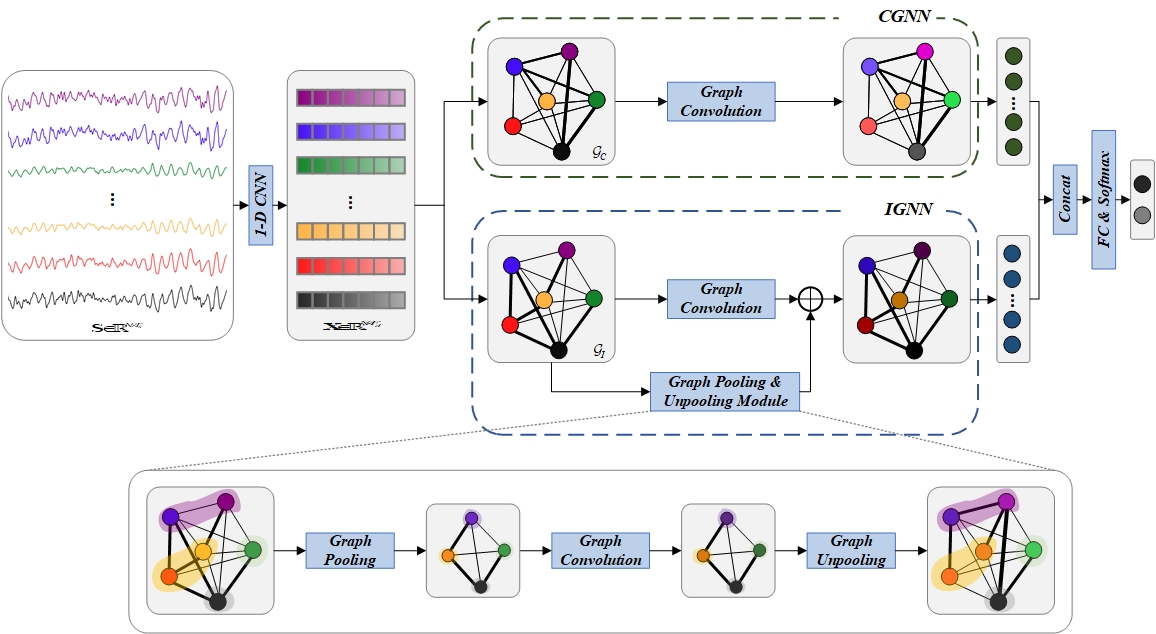
Figure 1: The framework of the proposed HybGNN

2.2 EEG Temporal Feature Extraction

1-D CNN has been widely used in multivariate time series, such as biomedical data, due to its competitive performance, as well as its real-time and low-cost hardware implementation compared to RNN-based methods[25]. We employ a 1-D CNN module to extract temporal dependencies within each electrode, which is operated on time dimension and ensures that the spatial information remains as it is, to construct a graph in the next step.

A raw EEG sample is denoted by $\boldsymbol{S}\in{\mathbb{R}}^{N\times{T_{s}}}$, where the sample originates from $N$ EEG electrodes and each electrode has $T_{s}$ time stamps. We use the 1-D CNN to extract temperal features from the raw EEG sample $\boldsymbol{S}$ and the output of 1-D CNN can be denoted as $\boldsymbol{X}\in{\mathbb{R}}^{N\times{F}_{d}}$, where $N$ is the number of EEG electrodes and ${F}_{d}$ is the number of features on each electrode.

2.3 CGNN and IGNN

2.3.1 Definition of Brain Network

A brain network can be defined as a graph in the form of $\mathcal{G}=\begin{Bmatrix}\mathcal{V},\mathcal{E},\boldsymbol{A}\end{Bmatrix}$, where $\mathcal{V}$ represents the set of nodes with the number of $\left|\mathcal{V}\right|=N$, and each node in the network represents an EEG electrode. $\mathcal{E}$ represents the set of edges, which indicates the relationships between the nodes. $\boldsymbol{A}\in{\mathbb{R}}^{N\times N}$ denotes the adjacency matrix, whose element ${a}_{ij}$ measures the importance of the connection between the $i$th node and the $j$th one. In our model, $\boldsymbol{X}\in{\mathbb{R}}^{N\times{F}_{d}}$, which denotes the EEG features matrix extracted by 1-D CNN above, is transformed into two graphs: ${\mathcal{G}}_{C}$ and ${\mathcal{G}}_{I}$. ${\mathcal{G}}_{C}$ denotes the graph in the CGNN and ${\mathcal{G}}_{I}$ denotes the graph in the IGNN.

2.3.2 Construction of CGNN

Previous researchers have identified several common abnormal patterns that indicate depression, which are shared by most patients and remain stable over time[41]. The existence of these common abnormalities greatly raises the probability of depression. To uncover these common abnormal patterns, we design a fixed graph connection.

However, due to the brain’s complexity and the unclear mechanisms of depression, direct definition of the fixed graph connections is difficult. Therefore, instead of attempting to define the fixed graph connection, we make it learnable through an adjacency matrix. This matrix enables the model to explore the common graph connection from the training data automatically. Once training is complete, the matrix becomes fixed and will be applied to all input instances. The common adjacency matrix can be denoted as ${\boldsymbol{A}}_{C}\in{\mathbb{R}}^{N\times N}$.

2.3.3 Construction of IGNN

To tackle the individual differences and reveal the individual-specific abnormal patterns for the detection of depression, we design the IGNN model, where the graph is constructed based on instance data. We already have $\boldsymbol{X}=\begin{Bmatrix}{x}_{m}^{T}\end{Bmatrix}_{m=1}^{N},x_{m}\in{\mathbb{R}}^{F_{d}}$, which represents the output from the 1-D CNN applied to each EEG channel. Then we use a graph construction function $h(x_{i},x_{j})$, to construct the similarities between the features of two nodes, thereby constructing the adjacency matrix. The element $a_{ij}$ in the adjacency matrix is defined by:

$$a_{ij}=softmax(h({x}_{i},{x}_{j}))=\frac{exp(h({x}_{i},{x}_{j}))}{\textstyle\sum_{i=1}^{N}exp(h({x}_{i},{x}_{j}))},$$

$$h({x}_{i},{x}_{j})=({x}_{i}^{T}{W}_{1})({x}_{j}^{T}{W}_{2})^{T},$$ (1)

where ${W}_{1}\in\mathbb{R}^{F_{d}\times F_{m}}$ and ${W}_{2}\in\mathbb{R}^{F_{d}\times F_{m}}$ are projection matrices. $exp(\cdot)$ denotes exponential function. Addtionally, the softmax function is applied to normalize these similarities between the two nodes, where the value of $a_{ij}$ is within the range of $[0,1]$. Then, we obtain the individualized adjacency matrix $A_{I}=\begin{Bmatrix}a_{ij}\end{Bmatrix}_{i,j=1}^{N}\in\mathbb{R}^{N\times N}$.

2.3.4 Graph Convolution in CGNN and IGNN

After the construction of the two graphs, we perform graph convolution operations within the two GNNs respectively to extract richer spatial features. Generally, GNNs perform a feature transformation on $X\in\mathbb{R}^{N\times F_{d}}$ and produce an output $Y\in\mathbb{R}^{N\times d}$, where $d$ represents the output feature dimension. We adopt the popular graph convolutional networks (GCNs)[30] and the transformation of the feature between adjacent layers of GCNs can be written as follows:

$$H^{(l)}=\sigma\left(\tilde{D}^{-\frac{1}{2}}\tilde{A}\tilde{D}^{-\frac{1}{2}}H^{(l-1)}W^{(l-1)}\right),$$ (2)

where $l=1,2,...,L$. $L$ denotes number of layers. $\tilde{A}=A+I$, $\tilde{D}=\sum_{j}\tilde{A}_{ij}$, $H^{(0)}=X$, $H^{(L)}=Y$. $H^{(l)}$ denotes the output of $l$ layers of GCNs. $W^{(l-1)}\in\mathbb{R}^{F_{d}\times d}$ denotes a trainable weight matrix at layer $l-1$. To capture different level information of the graph, the $L$ step graph convolutional operations can be defined as:

$${f}_{GCN}^{L}=\displaystyle\sum_{l=0}^{L}\hat{A}^{l}XW^{(l)},$$ (3)

where $\hat{A}=\tilde{D}^{-\frac{1}{2}}\tilde{A}\tilde{D}^{-\frac{1}{2}}$, $W^{(l)}\in\mathbb{R}^{{F_{d}}\times{d}}$ denotes a linear transformation in layer $l$. Then, the output of the graph convolution in the two branches above can be defined as follows:

$$Y_{C}=\displaystyle\sum_{l=0}^{L}\hat{A}_{C}^{l}XW_{F}^{(l)},$$

$$Y_{I}=\displaystyle\sum_{l=0}^{L}\hat{A}_{I}^{l}XW_{I}^{(l)},$$ (4)

where $Y_{C}\in\mathbb{R}^{{N}\times{d}}$ and $Y_{I}\in\mathbb{R}^{{N}\times{d}}$ denote the graph convolution results of CGNN and IGNN respectively. $W_{C}^{(l)}\in\mathbb{R}^{F_{d}\times{d}}$ and $W_{I}^{(l)}\in\mathbb{R}^{F_{d}\times{d}}$ denote linear transformation in each branch.

2.4 Graph Pooling and Unpooling Module

Hierarchical structure refers to the arrangement from channel-level graph to region-level graph. In order to extract individualized hierarchical information, we embed a graph pooling and unpooling module (GPUM) into the IGNN, which is illustrated in Fig.1. Since how to partition EEG channels into brain regions is not well-defined, we propose an adaptive pooling operation to automatically determine these brain regions instead of manually defining them.

In graph pooling, an assignment matrix is learned that takes into account both the adjacency matrix and the node features. Suppose that the number of nodes is $N$, the number of regions is $N_{r}$, and the assignment matrix is denoted as $R\in\mathbb{R}^{N\times N_{r}}$. Each row of the assignment matrix represents an original node and each column represents a region. $R$ performs a assignment of each original node to a region. This assignment varies adaptively according to the EEG instances, defined as

$$R=softmax(\hat{A_{I}}XQ),$$ (5)

where $X\in\mathbb{R}^{N\times F_{d}}$ is the input features, $\hat{A_{I}}$ is the normalized adjacency matrix defined above in the IGNN and $Q\in\mathbb{R}^{F_{d}\times N_{r}}$ denotes the parameter matrix to fuse the features. The assignment matrix $R$ generates a new coarsened adjacency matrix representing the relationships between the regions and a new matrix of embeddings for the each region:

$$A_{r}=R^{T}A_{I}R\in\mathbb{R}^{N_{r}\times N_{r}},$$

$$X_{r}=R^{T}{X}\in\mathbb{R}^{N_{r}\times F_{d}},$$ (6)

where $A_{r}$ denotes the adjacency matrix in the graph of regions and $X_{r}$ denotes the features of the regions. Then a ${L}^{\prime}$ step graph convolution is performed on the regions and the result of the operation $Y_{r}\in\mathbb{R}^{N_{r}\times d}$ is defined by:

$$Y_{r}=\displaystyle\sum_{l^{\prime}=0}^{{L}^{\prime}}\hat{A}_{r}^{{l}^{\prime}}{X_{r}}W_{r}^{(l^{\prime})},$$ (7)

where $W_{r}^{(l^{\prime})}\in{\mathbb{R}}^{F_{d}\times d}$ denotes the parameter matrix. To combine the features of regions with original graph features, a graph unpooling operation is introduced using the assignment matrix $R$ and the result can be denoted as:

$$Y_{r}^{\prime}=RY_{r}\in\mathbb{R}^{N\times d}.$$ (8)

Then, with the same dimension, we can merge the information of brain regions to the original graph features. The output of IGNN with GPUM and the final output of the two graph models is formulated as:

$$Y_{I}^{\prime}=Y_{I}\oplus Y_{r}^{\prime}\in\mathbb{R}^{N\times d},$$

$$Y_{all}=[Y_{I}^{\prime}\mid\mid Y_{C}]\in\mathbb{R}^{N\times 2d},$$ (9)

where $\oplus$ denotes the element-wise addition, $\mid\mid$ denotes the concatenation operator, $Y_{I}^{\prime}$ denotes the output of IGNN with the GPUM, $Y_{I}$ denotes the output of IGNN without the GPUM, $Y_{C}$ denotes the output of CGNN above and $Y_{all}$ denotes the final output of two GNNs.

2.5 Loss Function

Note that the membership for each brain region should be clearly defined, i.e., one node comes to one region in assignment matrix $R$. So an entropy minimization regularization is composed to each row of $R$, encouraging the rows to be approximately one-hot vectors[23]. Consequently, our model aims to minimize both the cross-entropy loss and the entropy minimization loss of the assignment matrix $R$. The loss can be formulated as follows:

$$\mathcal{L}=-\sum_{c=1}^{C}y_{c}\log\hat{y}_{c}-\lambda\sum_{i=1}^{N}\sum_{j=1}^{N_{r}}R_{ij}\log R_{ij},$$ (10)

where $C$ denotes number of classes, $y_{c}\in\{0,1\}$, $\hat{y}_{c}\in[0,1]$. If the sample belongs to the $c$-th class, then $y_{c}=1$, otherwise $y_{c}=0$. $\hat{y}_{c}$ represents the predicted probability that the sample is classified into the $c$-th class. The second term is the entropy minimization loss, where $\lambda$ is the regularization coefficient, $N$ is the number of nodes and $N_{r}$ is the number of regions.

3 Experiments

3.1 Datasets and preprocessing

Two public datasets are used to validate the effectiveness of the proposed model. We mainly focus on the resting-state EEG data in the two datasets.

1)MODMA: Multi-modal Open Dataset for Mental Disorder Analysis (MODMA)[32] consists of EEG data from 24 depression patients and 29 healthy controls(HCs). Each subject has 5 minutes of resting-state data acquired by an EEG cap with 128 channels.

2)HUSM: The Hospital University Sains Malaysia (HUSM)[34] dataset conprises EEG data from 34 depression patients and 30 HCs. Each participant was recorded for two conditions with a 19-channels EEG cap: 5 minutes with eyes closed and 5 minutes with eyes open.

We first perform pre-processing following the previous studies[14]. For the MODMA dataset, we only use the 19 channels in the 10-20 system to evaluate the generalizability of our method and to be consistent with HUSM dataset. We follow the previous study[14] to divide the EEG signals into multiple fragments and each fragment has data of 4 s with 75% overlap, based on which we obtain 6864 MDD segments and 8294 HC segments. For the HUSM dataset, we divided the EEG recordings into non-overlapping 4-second segments and combined the eyes-closed and eyes-open data. After removing subjects with missing data, we obtained 3726 MDD segments and 3588 HC segments.

3.2 Implementation Details

We follow previous studies[10, 20, 13] and perform a ten-fold cross-validation on each dataset to obtain reliable evaluation results. Furthermore, to prevent information leakage, the data from a subject is used exclusively in either the training set or the test set. To thoroughly assess depression detection performance, accuracy (ACC), recall (REC), precision (PRE), and F1 score (F1) are used as evaluation metrics in experiments.

We implement HybGNN using PyTorch libraries[49] on a NVIDIA GeForce RTX 4060. For the MODMA dataset, the learning rate is set to 0.09, the maximum number of epochs is set to 100 and the number of regions $N_{r}$ is set to 5. For the HUSM dataset, the learning rate is set to 0.001, the maximum number of epochs is set to 60 and the $N_{r}$ is set to 4. For both datasets, the number of GCN layers $L$ in two branches is set to $2$, and the number of GCN layers $L^{\prime}$ in GPUM is set to $1$. The batch size is set to 128, and the regularization coefficient $\lambda$ is set to $10^{-5}$.

3.3 Compared method

To evaluate the proposed HybGNN model, we perform a quantitative comparison with several other approaches applied in the depression detection as well as those popular in other EEG tasks: EEGNet[26], DeprNet[14], GCN[30], DGCNN[28], MSTGNN[33], SGP[13], IGCNN[10], SDGCN[20]. Notably, EEGNet and DeprNet are CNN-based, while the others are GNN-based. For the aforementioned GNN-based approaches, all graph models employ the same 1-D CNN (proposed in Sec 2.2) as the temporal feature extractor. To ensure a convincing comparison with the proposed method, we directly run (or reproduce) the codes of the compared methods on our datasets.

4 Results and Discussion

4.1 Comparison of Depression Detection Performance

The results of the detection performance comparison on the MODMA and HUSM datasets are summarized in Table 1. Our proposed model outperforms other methods across most metrics on both datasets, demonstrating its effectiveness in depression detection. Specifically, our HybGNN achieves superior detection results. On the MODMA dataset, it gains a 1.69% higher accuracy and a 0.017 higher F1 score compared to SDGCN, which achieves the second-best result on this dataset. Similarly, on the HUSM dataset, HybGNN achieves a 1.45% higher accuracy and a 0.025 higher F1 score compared to IGCNN. Although they are all graph-based approaches, our model stands out in its ability to represent the brain connection better and integrate hierarchical information.

Our model improves EEG-based detection on MODMA and HUSM dataset, achieving the highest accuracy (95.42% on MODMA, 93.50% on HUSM), precision (94.44% on MODMA, 93.37% on HUSM), and F1 score (0.955 on MODMA, 0.941 on HUSM). While DGCNN achieves the highest recall on MODMA (98.19%), our model still performs competitively with a recall of 97.18%.

Table 1: Comparison of detection performance on the MODMA and HUSM datasets

Methods	MODMA				HUSM
	ACC(%)	REC(%)	PRE(%)	F1	ACC(%)	REC(%)	PRE(%)	F1
EEGNet [26]	86.45	88.45	87.98	0.858	81.26	78.83	76.14	0.761
DeprNet [14]	90.06	92.39	88.46	0.897	87.68	91.20	84.68	0.874
SGP [13]	73.99	72.51	74.63	0.722	90.49	84.70	89.69	0.856
GCN [30]	89.48	93.38	86.02	0.887	90.13	94.05	87.95	0.904
DGCNN [28]	91.48	98.19	86.35	0.911	91.06	91.28	92.88	0.915
IGCNN [10]	92.89	97.02	90.40	0.933	92.05	90.80	91.27	0.916
MSTGNN [33]	93.14	93.47	92.70	0.927	90.90	89.63	90.91	0.900
SDGCN [20]	93.73	97.23	91.20	0.938	90.73	90.19	92.42	0.907
Ours	95.42	97.18	94.44	0.955	93.50	95.91	93.37	0.941

4.2 Ablation Studies

To further verify the validity of the key components in our model, we conduct an ablation study. In the experiment, we initially consider the CGNN as the baseline framework. Subsequently, we progressively integrate additional components, including CGNN, IGNN (without GPUM) and GPUM to construct the proposed model. Additionally, we explore the optimal integration of the GPUM module.

Specifically, Variant a, b, c are generated to verify the effectiveness of CGNN, IGNN (without GPUM) and GPUM respectively, with Variant a serving as the baseline. Variant d, e are generated to explore the optimal integration of the GPUM and compare with our HGNN. The specific process is described as follows:

• Variant a: CGNN without GPUM.

• Variant b: IGNN without GPUM.

• Variant c: CGNN without GPUM + IGNN without GPUM.

• Variant d: CGNN with GPUM + IGNN without GPUM.

• Variant e: CGNN with GPUM + IGNN with GPUM.

• Ours: CGNN without GPUM + IGNN with GPUM.

The results are shown in Table 2. Firstly, by comparing the Variant a, b with Variant c, we notice a decrease in depression detection accuracy on both datasets without CGNN or IGNN. This leads us to conclude that CGNN and IGNN together improve the accuracy of depression detection. Secondly, Comparing the Variant c with our model reveals that GPUM module effectively aids in extracting hierarchical information, thereby improving depression detection accuracy. Additionally, by comparing the Variant d, e with our model, we infer that integrating GPUM with the IGNN yields the best performance. This proves that hierarchical information based on individualized graph connections is more discriminative. In summary, the ablation study demonstrates the effectiveness of each key component in our model.

Table 2: The results of the ablation study

Methods	MODMA				HUSM
	ACC(%)	REC(%)	PRE(%)	F1	ACC(%)	REC(%)	PRE(%)	F1
Variant a	91.91	95.43	88.78	0.913	91.56	91.71	92.49	0.918
Variant b	93.72	95.60	93.82	0.943	92.05	92.90	92.73	0.926
Variant c	94.58	96.96	93.10	0.948	92.21	96.78	90.77	0.934
Variant d	94.96	95.34	94.41	0.949	92.94	94.21	92.85	0.931
Variant e	94.24	96.99	93.92	0.951	93.38	95.45	93.54	0.940
Ours	95.42	97.18	94.44	0.955	93.50	95.91	93.37	0.941

4.3 Hyperparameter Optimization

The outcomes of hyperparameter optimization are depicted in Figure 2. Regarding the number of regions $N_{r}$, the proposed model maintains optimal performance for HUSM at $N_{r}=4$, and for MODMA at $N_{r}=5$. Regarding the regularization coefficient $\lambda$, the proposed model obtains the best performance at $\lambda=10^{-5}$ for the both datasets.

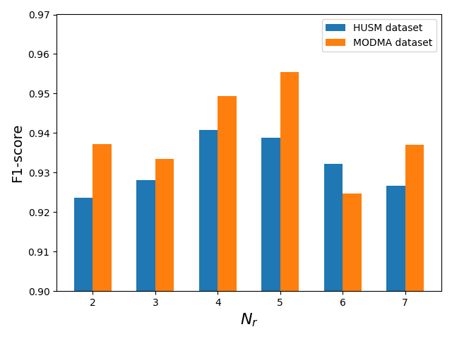
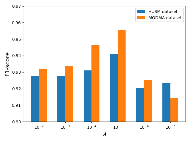
Figure 2: Hyperparameter optimization for the number of regions $N_{r}$ and regularization coefficient $\lambda$

5 Conclusion

In this paper, we introduce a hybrid graph neural network (HybGNN) for depression detection using EEG data. Our HybGNN framework incorporates both a common graph neural network (CGNN) branch and an individualized graph neural network (IGNN) branch to identify depression-related patterns while accommodating individual variations. Additionally, the IGNN includes a graph pooling and unpooling module (GPUM) to extract individualized hierarchical information. Extensive experiments on two public datasets demonstrate that HybGNN achieves state-of-the-art performance.

5.0.1

The authors have no competing interests to declare that are relevant to the content of this article.

References

- [1] Fava, M., Kendler, K.S.: Major depressive disorder. Neuron 28(2), 335–341 (2000)
- [2] Otte, C., Gold, S.M., Penninx, B.W., Pariante, C.M., Etkin, A., Fava, M., Mohr, D.C., Schatzberg, A.F.: Major depressive disorder. Nature reviews Disease primers 2(1), 1–20 (2016)
- [3] Seedat, S., Scott, K.M., Angermeyer, M.C., Berglund, P., Bromet, E.J., Brugha, T.S., Demyttenaere, K., De Girolamo, G., Haro, J.M., Jin, R., et al.: Cross-national associations between gender and mental disorders in the world health organization world mental health surveys. Archives of general psychiatry 66(7), 785–795 (2009)
- [4] Cummins, N., Sethu, V., Epps, J., Williamson, J.R., Quatieri, T.F., Krajewski, J.: Generalized two-stage rank regression framework for depression score prediction from speech. IEEE Transactions on Affective Computing 11(2), 272–283 (2017)
- [5] Chen, J., Lv, Y.n., Li, X.b., Xiong, J.j., Liang, H.t., Xie, L., Wan, C.y., Chen, Y.q., Wang, H.s., Liu, P., et al.: Urinary metabolite signatures for predicting elderly stroke survivors with depression. Neuropsychiatric Disease and Treatment pp. 925–933 (2021)
- [6] Calear, A.L., Christensen, H.: Systematic review of school-based prevention and early intervention programs for depression. Journal of adolescence 33(3), 429–438 (2010)
- [7] Acharya, U.R., Sudarshan, V.K., Adeli, H., Santhosh, J., Koh, J.E., Adeli, A.: Computer-aided diagnosis of depression using eeg signals. European neurology 73(5-6), 329–336 (2015)
- [8] Peng, H., Xia, C., Wang, Z., Zhu, J., Zhang, X., Sun, S., Li, J., Huo, X., Li, X.: Multivariate pattern analysis of eeg-based functional connectivity: A study on the identification of depression. Ieee Access 7, 92630–92641 (2019)
- [9] Zhang, B., Cai, H., Song, Y., Tao, L., Li, Y.: Computer-aided recognition based on decision-level multimodal fusion for depression. IEEE Journal of Biomedical and Health Informatics 26(7), 3466–3477 (2022)
- [10] Zhu, J., Jiang, C., Chen, J., Lin, X., Yu, R., Li, X., Hu, B.: Eeg based depression recognition using improved graph convolutional neural network. Computers in Biology and Medicine 148, 105815 (2022)
- [11] Shen, J., Zhang, Y., Liang, H., Zhao, Z., Zhu, K., Qian, K., Dong, Q., Zhang, X., Hu, B.: Depression recognition from eeg signals using an adaptive channel fusion method via improved focal loss. IEEE Journal of Biomedical and Health Informatics (2023)
- [12] Shen, J., Zhang, Y., Liang, H., Zhao, Z., Dong, Q., Qian, K., Zhang, X., Hu, B.: Exploring the intrinsic features of eeg signals via empirical mode decomposition for depression recognition. IEEE Transactions on Neural Systems and Rehabilitation Engineering 31, 356–365 (2022)
- [13] Chen, T., Guo, Y., Hao, S., Hong, R.: Exploring self-attention graph pooling with eeg-based topological structure and soft label for depression detection. IEEE transactions on affective computing 13(4), 2106–2118 (2022)
- [14] Seal, A., Bajpai, R., Agnihotri, J., Yazidi, A., Herrera-Viedma, E., Krejcar, O.: Deprnet: A deep convolution neural network framework for detecting depression using eeg. IEEE Transactions on Instrumentation and Measurement 70, 1–13 (2021)
- [15] Sharma, G., Joshi, A.M., Gupta, R., Cenkeramaddi, L.R.: Depcap: a smart healthcare framework for eeg based depression detection using time-frequency response and deep neural network. IEEE Access (2023)
- [16] Wang, D., Lei, C., Zhang, X., Wu, H., Zheng, S., Chao, J., Peng, H.: Identification of depression with a semi-supervised gcn based on eeg data. In: 2021 IEEE International Conference on Bioinformatics and Biomedicine (BIBM). pp. 2338–2345. IEEE (2021)
- [17] Shen, J., Chen, J., Ma, Y., Cao, Z., Zhang, Y., Hu, B.: Explainable depression recognition from eeg signals via graph convolutional network. In: 2023 IEEE International Conference on Bioinformatics and Biomedicine (BIBM). pp. 1406–1412. IEEE (2023)
- [18] Yu, M., Hillebrand, A., Tewarie, P., Meier, J., van Dijk, B., Van Mieghem, P., Stam, C.J.: Hierarchical clustering in minimum spanning trees. Chaos: An Interdisciplinary Journal of Nonlinear Science 25(2) (2015)
- [19] Li, X., Jing, Z., Hu, B., Zhu, J., Zhong, N., Li, M., Ding, Z., Yang, J., Zhang, L., Feng, L., et al.: A resting-state brain functional network study in mdd based on minimum spanning tree analysis and the hierarchical clustering. Complexity 2017 (2017)
- [20] Cui, W., Sun, M., Dong, Q., Guo, Y., Liao, X.F., Li, Y.: A multiview sparse dynamic graph convolution-based region-attention feature fusion network for major depressive disorder detection. IEEE Transactions on Computational Social Systems (2023)
- [21] Venkatapathy, S., Votinov, M., Wagels, L., Kim, S., Lee, M., Habel, U., Ra, I.H., Jo, H.G.: Ensemble graph neural network model for classification of major depressive disorder using whole-brain functional connectivity. Frontiers in Psychiatry 14, 1125339 (2023)
- [22] Jiang, X., Shen, Y., Yao, J., Zhang, L., Xu, L., Feng, R., Cai, L., Liu, J., Chen, W., Wang, J.: Connectome analysis of functional and structural hemispheric brain networks in major depressive disorder. Translational psychiatry 9(1), 136 (2019)
- [23] Ying, Z., You, J., Morris, C., Ren, X., Hamilton, W., Leskovec, J.: Hierarchical graph representation learning with differentiable pooling. Advances in neural information processing systems 31 (2018)
- [24] Gao, H., Ji, S.: Graph u-nets. In: international conference on machine learning. pp. 2083–2092. PMLR (2019)
- [25] Kiranyaz, S., Avci, O., Abdeljaber, O., Ince, T., Gabbouj, M., Inman, D.J.: 1d convolutional neural networks and applications: A survey. Mechanical systems and signal processing 151, 107398 (2021)
- [26] Lawhern, V.J., Solon, A.J., Waytowich, N.R., Gordon, S.M., Hung, C.P., Lance, B.J.: Eegnet: a compact convolutional neural network for eeg-based brain–computer interfaces. Journal of neural engineering 15(5), 056013 (2018)
- [27] Salvador, R., Suckling, J., Coleman, M.R., Pickard, J.D., Menon, D., Bullmore, E.: Neurophysiological architecture of functional magnetic resonance images of human brain. Cerebral cortex 15(9), 1332–1342 (2005)
- [28] Song, T., Zheng, W., Song, P., Cui, Z.: Eeg emotion recognition using dynamical graph convolutional neural networks. IEEE Transactions on Affective Computing 11(3), 532–541 (2018)
- [29] Vaswani, A., Shazeer, N., Parmar, N., Uszkoreit, J., Jones, L., Gomez, A.N., Kaiser, Ł., Polosukhin, I.: Attention is all you need. Advances in neural information processing systems 30 (2017)
- [30] Kipf, T.N., Welling, M.: Semi-supervised classification with graph convolutional networks. arXiv preprint arXiv:1609.02907 (2016)
- [31] Meunier, D., Lambiotte, R., Bullmore, E.T.: Modular and hierarchically modular organization of brain networks. Frontiers in neuroscience 4, 7572 (2010)
- [32] Cai, H., Gao, Y., Sun, S., Li, N., Tian, F., Xiao, H., Li, J., Yang, Z., Li, X., Zhao, Q., et al.: Modma dataset: A multi-modal open dataset for mental-disorder analysis. arxiv 2020. arXiv preprint arXiv:2002.09283
- [33] Jia, Z., Lin, Y., Wang, J., Ning, X., He, Y., Zhou, R., Zhou, Y., Li-wei, H.L.: Multi-view spatial-temporal graph convolutional networks with domain generalization for sleep stage classification. IEEE Transactions on Neural Systems and Rehabilitation Engineering 29, 1977–1986 (2021)
- [34] Mumtaz, W., Xia, L., Mohd Yasin, M.A., Azhar Ali, S.S., Malik, A.S.: A wavelet-based technique to predict treatment outcome for major depressive disorder. PloS one 12(2), e0171409 (2017)
- [35] Hu, J., Shen, L., Sun, G.: Squeeze-and-excitation networks. In: Proceedings of the IEEE conference on computer vision and pattern recognition. pp. 7132–7141 (2018)
- [36] Chollet, F.: Xception: Deep learning with depthwise separable convolutions. In: Proceedings of the IEEE conference on computer vision and pattern recognition. pp. 1251–1258 (2017)
- [37] Grattarola, D., Zambon, D., Bianchi, F.M., Alippi, C.: Understanding pooling in graph neural networks. IEEE transactions on neural networks and learning systems (2022)
- [38] Bullmore, E., Sporns, O.: Complex brain networks: graph theoretical analysis of structural and functional systems. Nature reviews neuroscience 10(3), 186–198 (2009)
- [39] Chen, C.H., Gutierrez, E., Thompson, W., Panizzon, M.S., Jernigan, T.L., Eyler, L.T., Fennema-Notestine, C., Jak, A.J., Neale, M.C., Franz, C.E., et al.: Hierarchical genetic organization of human cortical surface area. Science 335(6076), 1634–1636 (2012)
- [40] Park, H.J., Friston, K.: Structural and functional brain networks: from connections to cognition. Science 342(6158), 1238411 (2013)
- [41] Mulders, P.C., van Eijndhoven, P.F., Schene, A.H., Beckmann, C.F., Tendolkar, I.: Resting-state functional connectivity in major depressive disorder: a review. Neuroscience & Biobehavioral Reviews 56, 330–344 (2015)
- [42] Kaiser, R.H., Whitfield-Gabrieli, S., Dillon, D.G., Goer, F., Beltzer, M., Minkel, J., Smoski, M., Dichter, G., Pizzagalli, D.A.: Dynamic resting-state functional connectivity in major depression. Neuropsychopharmacology 41(7), 1822–1830 (2016)
- [43] Song, T., Liu, S., Zheng, W., Zong, Y., Cui, Z.: Instance-adaptive graph for eeg emotion recognition. In: Proceedings of the AAAI Conference on Artificial Intelligence. vol. 34, pp. 2701–2708 (2020)
- [44] Xue, Y., Zheng, W., Zong, Y., Chang, H., Jiang, X.: Adaptive hierarchical graph convolutional network for eeg emotion recognition. In: 2022 International Joint Conference on Neural Networks (IJCNN). pp. 1–8. IEEE (2022)
- [45] Jia, Z., Lin, Y., Wang, J., Zhou, R., Ning, X., He, Y., Zhao, Y.: Graphsleepnet: Adaptive spatial-temporal graph convolutional networks for sleep stage classification. In: IJCAI. vol. 2021, pp. 1324–1330 (2020)
- [46] Luo, G., An, P., Li, Y., Hong, R., Chen, S., Rao, H., Chen, W.: Exploring adaptive graph topologies and temporal graph networks for eeg-based depression detection. IEEE Transactions on Neural Systems and Rehabilitation Engineering (2023)
- [47] Beijers, L., Wardenaar, K.J., van Loo, H.M., Schoevers, R.A.: Data-driven biological subtypes of depression: systematic review of biological approaches to depression subtyping. Molecular psychiatry 24(6), 888–900 (2019)
- [48] Klepl, D., Wu, M., He, F.: Graph neural network-based eeg classification: A survey. IEEE Transactions on Neural Systems and Rehabilitation Engineering (2024)
- [49] Paszke, A., Gross, S., Massa, F., Lerer, A., Bradbury, J., Chanan, G., Killeen, T., Lin, Z., Gimelshein, N., Antiga, L., et al.: Pytorch: An imperative style, high-performance deep learning library. Advances in neural information processing systems 32 (2019)