Fast and Efficient Bayesian Analysis of Structural Vector Autoregressions Using the R Package bsvars (Version 3.2)

Tomasz Woźniak Fast and Efficient Bayesian Analysis of Structural Vector Autoregressions Using the R Package bsvars bsvars: Bayesian Estimation of Structural Vector Autoregressions The R package bsvars provides a wide range of tools for empirical macroeconomic and financial analyses using Bayesian Structural Vector Autoregressions. It uses frontier econometric techniques and C++ code to ensure fast and efficient estimation of these multivariate dynamic structural models, possibly with many variables, complex identification strategies, and non-linear characteristics. The models can be identified using adjustable exclusion restrictions and heteroskedastic or non-normal shocks. They feature a flexible three-level equation-specific local-global hierarchical prior distribution for the estimated level of shrinkage for autoregressive and structural parameters. Additionally, the package facilitates predictive and structural analyses such as impulse responses, forecast error variance and historical decompositions, forecasting, statistical verification of identification and hypotheses on autoregressive parameters, and analyses of structural shocks, volatilities, and fitted values. These features differentiate bsvars from existing R packages that either focus on a specific structural model, do not consider heteroskedastic shocks, or lack the implementation using compiled code. Bayesian inference, Structural VARs, Gibbs sampler, exclusion restrictions, heteroskedasticity, non-normal shocks, forecasting, structural analysis, R Bayesian inference, Structural VARs, Gibbs sampler, exclusion restrictions, heteroskedasticity, non-normal shocks, forecasting, structural analysis, R Tomasz Woźniak
University of Melbourne
Department of Economics
111 Barry Street
3053 Carlton, VIC, Australia
E-mail:
URL: https://bsvars.org
 

1 Introduction

Since the publication of the seminal paper by Sims (1980) Structural Vector Autoregressions (SVARs) have become benchmark models for empirical macroeconomic analyses. Subsequently, they have found numerous applications in other fields and are now indispensable in everyday work at central banks, treasury departments and other economic governance institutions, as well as in finance, insurance, banking, and economic consulting.

The great popularity of these multivariate dynamic structural models was gained because they incorporate the reduced and structural forms into a unified framework. On the one hand, they capture the essential properties of macroeconomic and financial time series such as persistence, dynamic effects, system modelling, and potentially time-varying conditional variances. On the other hand, they control for the structure of an economy, system, or market through the contemporaneous effects and, thus, they identify contemporaneously and temporarily uncorrelated shocks that can be interpreted structurally. All these features make it possible to estimate the dynamic causal effects of the shocks on the measurements of interest reliably. These effects are interpreted as the propagation of the well-isolated and unanticipated cause – a structural shock – in the considered system of variables throughout the predictable future.

This flexibility comes at a cost of dealing with local identification of the model, sharply growing dimension of the parameter space with the increasing number of variables, and the estimation of latent variables. Bayesian inference provides original solutions to each of these challenges often deciding on the feasibility of the analyses with a demanded model including many variables, conditional heteroskedasticity, and sophisticated identification of the structural shocks. In this context, Markov Chain Monte Carlo methods grant certainty of reliable estimation thanks to simple convergence diagnostics but they might incur substantial computational cost.

The paper at hand and the corresponding package bsvars by Woźniak (2024) for R (R Core Team, 2021) provide tools for empirical macroeconomic and financial analyses using Bayesian SVARs. It addresses the considered challenges by choosing a convenient model formulation, applying frontier econometric and numerical techniques, and relying on compiled code written using C++ to ensure fast and efficient estimation. Additionally, it offers a great flexibility in choosing the model specification and identification pattern, modifying the prior assumptions, and accessing interpretable tabulated or plotted outputs. Therefore, the package makes it possible to benefit from the best of the two facilities: the convenience of data analysis using R and the computational speed using pre-compiled code written in C++.

More specifically, the package uses the SVAR models featuring a standard reduced form VAR equation following Bańbura et al. (2010) (see also Woźniak, 2016) and a structural equation linking the reduced form error term to the structural shocks via the structural matrix as in Lütkepohl et al. (2024) and Chan et al. (2024). The normal prior distribution for the autoregressive parameters implements the interpretability of the Minnesota prior by Doan et al. (1984) by centring it around the mean that reflects unit-root nonstationarity or stationarity of the variables with an adjustable level of shrinkage depending on the equation and exhibiting exponential decay with the increasing autoregressive lag order. The prior distribution for the structural matrix is generalised-normal by Waggoner and Zha (2003a) which preserves the shape of the likelihood function (see Woźniak and Droumaguet, 2015). Both of these priors are combined with the flexible three-level equation-specific local-global hierarchical prior distribution for the estimated level of shrinkage as in Lütkepohl et al. (2024) improving the model fit. The estimation of the level of shrinkage was shown to substantially improve forecasting performance of VAR models by Giannone et al. (2015). Additionally, these specification choices lead to an efficient equation-by-equation Gibbs sampler for the posterior distribution of the autoregressive and structural parameters proposed by Chan et al. (2024) and Waggoner and Zha (2003a) respectively.

Figure 1: The hexagonal package logo features an impulse response that can be fully reproduced using the bsvars package following a script available at: github.com/bsvars/hex/blob/main/bsvars/bsvars.R

All the structural models in the bsvars package can be identified using highly adaptable exclusion restrictions proposed by Waggoner and Zha (2003a) and use the structural matrix sign normalisation by Waggoner and Zha (2003b). However, one might also choose to include additional sources of identification through heteroskedasticity following the ideas by Rigobon (2003) or by non-normal shocks as proposed by Lanne and Lütkepohl (2010). Therefore, the package offers a range of models for structural shocks conditional variance including a homoskedastic model with time-invariant variances. The list of heteroskedastic specifications is opened by Stochastic Volatility (SV) model in two versions: non-centred as in Lütkepohl et al. (2024) and centred used by Chan et al. (2024), and is followed by the Markov-switching heteroskedasticity (MSH) model proposed by Brunnermeier et al. (2021). The implementations of the MSH models follows that by Woźniak and Droumaguet (2015) in two versions: with stationary Markov process and its sparse version that facilitates the estimation of the number of states and non-parametric interpretations. Similarly, models with non-normal shocks are implemented in three versions including Student-t distributed shocks proposed by Lanne et al. (2017), and those following the normal mixture (MIX) model: with a finite number of components as in Frühwirth-Schnatter (2006) and in its sparse representation serving as an approximation of a non-parametric infinite mixture inspired by Malsiner-Walli et al. (2016).

The R package bsvars implements a wide range of tools for structural and predictive analyses. The former encompasses the methods comprehensively revised by (Kilian and Lütkepohl, 2017, Chapter 4: SVAR Tools) and include the impulse response functions, forecast error variance decompositions, historical decompositions, as well as the basic analysis of fitted values, structural shocks, conditional standard deviations and regime probabilities for MSH and MIX models. The predictive analysis includes Bayesian forecasting implemented through an algorithm sampling from the predictive density of the unknown future values of the dependent variables, and conditional forecasting of a number of variables given other variables’ projections. Methods summary() and plot() support the user in the interpretations and visualisation of such analyses.

A distinguishing feature of the package are the Bayesian model diagnostic tools for the verification of identification and hypotheses on autoregressive parameters using posterior odds ratios. The posterior odds for hypotheses expressed as sharp restrictions on parameters are computed using Savage-Dickey Density Ratios (SDDRs) by Verdinelli and Wasserman (1995). The SDDRs representing Bayes factors are reliable, precisely estimated, and straightforward to compute once the posterior sample is available. As shown by Lütkepohl and Woźniak (2020) and Lütkepohl et al. (2024), SDDRs are a pragmatic tool for the Bayesian assessment of a null hypothesis of homoskedasticity in heteroskedastic models allowing to verify partial or global identification through heteroskedasticity. A similar argument applies for the verification of identification in non-normal models. Additionally, the package’s general implementation of SDDRs for the autoregressive parameters facilitates verification of restrictions on any conditional mean parameters of the model, such as e.g., hypotheses of exogeneity or Granger non-causality.

Finally, the package bsvars is highly integrated in terms of workflows, objects, and code compatibility with an R package bsvarSIGNs by Wang and Woźniak (2024) focusing on SVAR models identified using sign (Rubio-Ramirez et al., 2010), sign and zero (Arias et al., 2018), and narrative restrictions (Antolín-Díaz and Rubio-Ramírez, 2018). The bsvarSIGNs package usage compatibility and its complementarity in terms of the implemented SVAR identification methods constitutes an additional appeal of the bsvars package.

Multivariate dynamic modelling, both Bayesian and frequentist, has found some traction in R in the recent years, which resulted in many new packages available on the CRAN repository. Two packages, MTS by Tsay et al. (2022) and vars by Pfaff (2008), cover a wide range of benchmark models for multivariate time series analysis in economics in finance. Other packages provide functionality for reduced-form models estimation and forecasting implementing regularisation, such as the BigVAR package by Nicholson et al. (2023), bigtime by Wilms et al. (2023), and VARshrink by Lee and Kim (2019), or Bayesian shrinkage, such as the bvartools package by Mohr (2022), bayesianVARs by Gruber (2024), or BGVAR by Boeck et al. (2020). All of these specification are proven to be highly beneficial for forecasting in particular contexts.

Notable implementations of structural models include packages focusing on specific models important from the point of view of historical developments in the field, namely, the package BVAR by Kuschnig and Vashold (2021) providing tools for the estimation and analysis proposed by Giannone et al. (2015), package bvarsv by Krueger (2015) focusing on the heteroskedastic VAR proposed by Primiceri (2005), and package FAVAR by Chen and Chen (2022) implementing the factor-augmented model by Bernanke et al. (2005). Other two packages that have been archived and are no longer available on CRAN are the package MSBVAR by Brandt (2006) focusing on the Markov switching model by Sims and Zha (2006) and package VARsignR by Danne (2015) provided a treatment of Bayesian SVARs identified via sign restrictions by Uhlig (2005), Rubio-Ramirez et al. (2010), and Fry and Pagan (2011). Some other packages focus on the implementation of research code for families of models focused around a theme, such as the aforementioned package bsvarSIGNs for sign-restricted SVARs, package gmvarkit by Virolainen (2024a) implementing frequentist SVARs with non-Gaussian identification by Kalliovirta et al. (2016) and Virolainen (2024d), or package sstvars by Virolainen (2024c) focusing on smooth-transition non-linearity in the structural models by Virolainen (2024b), Anderson and Vahid (1998), and Lütkepohl and Netšunajev (2017). Importantly, there exists a whole universe of MATLAB libraries for structural macroeconomics analyses. However, the code is available mostly from authors’ websites and without structured documentation. This family of libraries is not surveyed here but we single out the BEAR toolkit by Dieppe and van Roye (2024) and Dynare by Dynare Team (2024) providing comprehensive set of methods and extensive documentation.

However, the most relevant package to compare bsvars to is the svars package by Lange et al. (2021) focusing on frequentist inference for SVAR models identified via exclusion restrictions, heteroskedasticity, and non-normal shocks and implementing a range of models that are feasible to estimate using the maximum likelihood method. The similarity to the functionality of package bsvars include the selection of models, such as the MSH and with non-normal residuals, as well as the selection of tools for structural analyses including impulse responses, historical and forecast error variance decompositions. However, the package svars implements maximum likelihood and bootstrap procedures for the analysis of the model parameters and offers some specification testing procedures.

In this context, the bsvars package implements a range of novel solutions and models for Bayesian analysis. One differentiating example is the implementation of the SVAR models with SV that is not covered by the package svars. This model is particularly important in the context of recent developments clearly indicating that SV is the single extension of VARs leading to marginally largest improvements in the model fit and forecasting performance as shown e.g. by Clark and Ravazzolo (2015), Chan and Eisenstat (2018), Carriero et al. (2019), Chan (2020), and Bertsche and Braun (2022). Another such example are sparse MSH and MIX models based on hierarchical prior structures deciding on their frequentist implementation infeasibility. Additionally, the package bsvars provides unique Bayesian statistical procedures for the verification of partial identification through heteroskedasticity and non-normality using method verify_identification(). The verification of identification for such flexible models as those considered in the package is not feasible in the frequentist framework. Finally, the package benefits from the advantage of Bayesian approach that facilitates the estimation for models with potentially many variables, autoregressive lags inflating the dimension of parameters space, Markov-switching regimes or normal mixture components, all of which are the factors constraining the feasibility of maximum likelihood approaches.

2 Bayesian Analysis of Structural VARs

This section scrutinises the modelling framework used in the package focusing on the specification of the models, prior distributions, hypotheses verification tools, and estimation. The reader is referred to (Kilian and Lütkepohl, 2017, Chapter 4: SVAR Tools) for the exposition of the standard tools for the analysis of SVAR models, such as the impulse responses, forecast error variance and historical decompositions, as their implementation in the package closely follows this resource.

2.1 Structural VARs

All of the models in the package bsvars share the reduced and structural form equations, as well as the hierarchical prior distributions for these parameters following Lütkepohl et al. (2024). The reduced form equation is the VAR equation with $p$ lags specified for an $N$-vector $\mathbf{y}_{t}$ collecting observations on $N$ variables at time $t$:

$$\mathbf{y}_{t} =\mathbf{A}_{1}\mathbf{y}_{t-1}+\dots+\mathbf{A}_{p}\mathbf{y}_{t-p}+\mathbf{A}_{d}\mathbf{d}_{t}+\boldsymbol{\varepsilon}_{t},$$ (1)

where $\mathbf{A}_{i}$ are $N\times N$ matrices of autoregressive slope parameters, $\mathbf{d}_{t}$ is a $D$-vector of deterministic terms, always including a constant term, and possibly dummy and exogenous variables, $\mathbf{A}_{d}$ is an $N\times D$ matrix of the corresponding parameters, and $\boldsymbol{\varepsilon}_{t}$ collects the $N$ reduced form error terms. Collect all the autoregressive matrices and the slope terms in an $N\times(Np+D)$ matrix $\mathbf{A}=\begin{bmatrix}\mathbf{A}_{1}&\dots&\mathbf{A}_{p}&\mathbf{A}_{d}\end{bmatrix}$ and the explanatory variables in a $(Np+D)$-vector $\mathbf{x}_{t}=\begin{bmatrix}\mathbf{y}_{t-1}^{\prime}&\dots&\mathbf{y}_{t-p}^{\prime}&\mathbf{d}_{t}^{\prime}\end{bmatrix}^{\prime}$. Then equation (1) can be written in the matrix form as

$$\mathbf{y}_{t} =\mathbf{A}\mathbf{x}_{t}+\boldsymbol{\varepsilon}_{t}.$$ (2)

Each of the rows of the matrix $\mathbf{A}$, denoted by $[\mathbf{A}]_{n\cdot}$ follows a multivariate conditional normal prior distribution, given the equation-specific shrinkage hyper-parameter $\gamma_{A.n}$, with the mean vector $\underline{\mathbf{m}}_{n.A}$ and the covariance $\gamma_{A.n}\underline{\Omega}_{A}$, denoted by:

$$[\mathbf{A}]_{n\cdot}^{\prime}\mid\gamma_{A.n}\sim\mathcal{N}_{Np+D}\left(\underline{\mathbf{m}}_{n.A},\gamma_{A.n}\underline{\boldsymbol{\Omega}}_{A}\right),$$ (3)

where $\underline{\mathbf{m}}_{n.A}$ is specified in-line with the Minnesota prior by Doan et al. (1984) as a vector of zeros if all of the variables are stationary, or containing value 1 in its $n\textsuperscript{th}$ element if the $n\textsuperscript{th}$ variable is unit-root nonstationary. By default, $\underline{\boldsymbol{\Omega}}_{A}$ is a diagonal matrix with vector $\begin{bmatrix}\mathbf{p}^{-2\prime}\otimes\boldsymbol{\imath}_{N}^{\prime}&100\boldsymbol{\imath}_{D}^{\prime}\end{bmatrix}^{\prime}$ on the main diagonal, where $\mathbf{p}$ is a vector containing a sequence of integers from 1 to $p$ and $\boldsymbol{\imath}_{N}$ is an $N$-vector of ones. Both, $\underline{\mathbf{m}}_{n.A}$ and $\underline{\boldsymbol{\Omega}}_{A}$ can be modified by the user. This specification includes the shrinkage level exponentially decaying with the increasing lag order, relatively large prior variances for the deterministic term parameters, and the flexibility of the hierarchical prior that leads to the estimation of the level of shrinkage as proposed by Giannone et al. (2015). The latter feature is facilitated by assuming a 3-level local-global hierarchical prior on the equation-specific reduced form parameters shrinkage given by

$$\gamma_{A.n}|s_{A.n} \sim\mathcal{IG}2\left(s_{A.n},\underline{\nu}_{A}\right),$$ (4)

$$s_{A.n}|s_{A} \sim\mathcal{G}\left(s_{A},\underline{a}_{A}\right),$$ (5)

$$s_{A} \sim\mathcal{IG}2\left(\underline{s}_{s_{A}},\underline{\nu}_{s_{A}}\right),$$ (6)

where $\mathcal{G}$ and $\mathcal{IG}2$ are gamma and inverted gamma 2 distributions (see Bauwens et al., 1999, Appendix A), hyper-parameters $\gamma_{A.n}$, $s_{A.n}$, and $s_{A}$ are estimated, and $\underline{\nu}_{A}$, $\underline{a}_{A}$, $\underline{s}_{s_{A}}$, and $\underline{\nu}_{s_{A}}$ are all set by default to value 10 to assure appropriate level of shrinkage towards the prior mean. The values of the hyper-parameters that are underlined in our notation can be modified by the user.

The structural form equation determines the linear relationship between the reduced-form innovations $\boldsymbol{\varepsilon}_{t}$ and the structural shocks $\mathbf{u}_{t}$ using the $N\times N$ structural matrix $\mathbf{B}_{0}$:

$$\mathbf{B}_{0}\boldsymbol{\varepsilon}_{t}=\mathbf{u}_{t}.$$ (7)

The structural matrix specifies the contemporaneous relationship between the variables in the system and determines the identification of the structural shocks from vector $\mathbf{u}_{t}$. Its appropriate construction may grant specific interpretation to one or many of the shocks. The package bsvars facilitates the identification of the structural matrix and the shocks via exclusion restrictions (see Kilian and Lütkepohl, 2017, Chapter 8) and/or through heteroskedasticity or non-normal shocks (Kilian and Lütkepohl, 2017, Chapter 14). The zero restrictions are imposed on the structural matrix row-by-row following the framework proposed by Waggoner and Zha (2003a) via the following decomposition of the $n\textsuperscript{th}$ row of the structural matrix, denoted by $[\mathbf{B}_{0}]_{n\cdot}$:

$$[\mathbf{B}_{0}]_{n\cdot}=\mathbf{b}_{n}\mathbf{V}_{n},$$ (8)

where $\mathbf{b}_{n}$ is a $1\times r_{n}$ vector collecting the elements to be estimated and the $r_{n}\times N$ matrix $\mathbf{V}_{n}$ including zeros and ones placing the estimated elements in the demanded elements of $[\mathbf{B}_{0}]_{n\cdot}$.

The structural matrix $\mathbf{B}_{0}$ follows a conditional generalised-normal prior distribution by Waggoner and Zha (2003a) recently revised by Arias et al. (2018) that is proportional to:

$$\mathbf{B}_{0}\mid\gamma_{B.1},\dots,\gamma_{B.N}\sim|\det(\mathbf{B}_{0})|^{\underline{\nu}_{B}-N}\exp\left\{-\frac{1}{2}\sum_{n=1}^{N}\gamma_{B.n}^{-1}\mathbf{b}_{n}\underline{\boldsymbol{\Omega}}_{B.n}^{-1}\mathbf{b}_{n}^{\prime}\right\},$$ (9)

where $\underline{\boldsymbol{\Omega}}_{B.n}$ is an $r_{n}\times r_{n}$ scale matrix set to the identity matrix by default, $\underline{\nu}_{B}\geq N$ is a shape parameter, and $\gamma_{B.n}$ is an equation-specific structural parameter shrinkage. The shape parameter $\underline{\nu}_{B}$ set to $N$ by default makes this prior a conditional, zero-mean $r_{n}$-variate normal prior distribution for $\mathbf{b}_{n}$ with the diagonal covariance and the diagonal element $\gamma_{B.n}$. The shape parameter can be modified by the user though.

This prior specification is complemented by a 3-level local-global hierarchical prior on the equation-specific structural parameters shrinkage given by

$$\gamma_{B.n}|s_{B.n} \sim\mathcal{IG}2\left(s_{B.n},\underline{\nu}_{b}\right),$$ (10)

$$s_{B.n}|s_{B} \sim\mathcal{G}\left(s_{B},\underline{a}_{B}\right),$$ (11)

$$s_{B} \sim\mathcal{IG}2\left(\underline{s}_{s_{B}},\underline{\nu}_{s_{B}}\right),$$ (12)

where hyper-parameters $\gamma_{B.n}$, $s_{B.n}$, and $s_{B}$ are estimated and $\underline{\nu}_{b}$, $\underline{a}_{B}$, $\underline{s}_{s_{B}}$, and $\underline{\nu}_{s_{B}}$ are fixed to values 10, 10, 1, and 100 respectively to assure a flexible dispersed distribution a priori but they can be modified by the user.

Finally, all of the models share the zero-mean conditional normality of the structural shocks given the past observations with the diagonal covariance matrix containing the $N$-vector of structural shock variances, $\boldsymbol{\sigma}_{t}^{2}$, on the main diagonal:

$$\mathbf{u}_{t}\mid\mathbf{x}_{t},\boldsymbol{\sigma}_{t}^{2}\sim\mathcal{N}_{N}\left(\mathbf{0}_{N},\text{diag}\left(\boldsymbol{\sigma}_{t}^{2}\right)\right).$$ (13)

The diagonal covariance matrix, together with the joint normality, implies contemporaneous independence of the structural shocks which is the essential feature allowing for the estimation of dynamic effects to a well-isolated cause that is not influenced by other factors in the SVAR models.

The model parts described in the current section are common to all the models considered in the package bsvars. Note that identification of the structural matrix here must be assured by the exclusion restrictions only in the homoskedastic model. Heteroskedastic and non-normal specifications might not require the exclusion restrictions to identify the structural matrix. Still, such restrictions might occur beneficial from the point of view of the model fit sharpening shock identification. Such alternative model specifications are distinguished by the characterisation of the conditional variances collected in vector $\boldsymbol{\sigma}_{t}^{2}$.

2.2 Models for Conditional Variances

The bsvars package offers a selection of alternative specifications for structural shocks conditional variance process.

2.2.1 Homoskedastic model

The first such specification is a homoskedastic model for which the conditional variance of every shock is equal to

$$\sigma_{n.t}^{2}=1$$ (14)

for all $t$. This setup results in a simple SVAR model that is quick to estimate. Note that in this model, the conditional covariance of the data vector, $\mathbf{y}_{t}$ is equal to $(\mathbf{B}_{0}^{\prime}\mathbf{B}_{0})^{-1}$. The point at which this model is standardized as in equation (14) is the benchmark value for the all other heteroskedastic models whose conditional variances hover around value 1.

2.2.2 Stochastic Volatility

The heteroskedastic model with Stochastic Volatility is implemented in two versions: non-centred by Lütkepohl et al. (2024) and centred Chan et al. (2024). In these models, the conditional variances for each of the shocks are given by

non-centred: $$\sigma_{n.t}^{2} =\exp\left\{\omega_{n}h_{n.t}\right\}$$ (15)

centred: $$\sigma_{n.t}^{2} =\exp\left\{\tilde{h}_{n.t}\right\},$$ (16)

where the parameter $\omega_{n}$ denotes the plus-minus square root of the conditional variance for the log-conditional variance process and will be referred to as the volatility of the log-volatility, whereas $h_{n.t}$ and $\tilde{h}_{n.t}$ are the log-volatility processes following autoregressive equations

non-centred: $$h_{n.t} =\rho_{n}h_{n.t-1}+v_{n.t}, v_{n.t}\sim\mathcal{N}\left(0,1\right)$$ (17)

centred: $$\tilde{h}_{n.t} =\rho_{n}\tilde{h}_{n.t-1}+\tilde{v}_{n.t}, \tilde{v}_{n.t}\sim\mathcal{N}\left(0,\sigma_{v}^{2}\right)$$ (18)

with the initial values $h_{n.0}=\tilde{h}_{n.0}=0$, where $\rho_{n}$ is the autoregressive parameter, $v_{n.t}$ and $\tilde{v}_{n.t}$ are the SV normal innovations, and $\sigma_{v}^{2}$ is the conditional variance of $\tilde{h}_{n.t}$ in the centred parameterisation.

The priors for these models include a uniform distribution for the autoregressive parameter

$$\rho_{n}\sim\mathcal{U}(-1,1),$$ (19)

which assures the stationarity of the log-volatility process and sets its unconditional expected value to $E[h_{n.t}]=E[\tilde{h}_{n.t}]=0$. The prior distribution for the volatility of the log-volatility parameter in the non-centred and the conditional variance of the log-volatility in the centred parameterisation follow a multi-level hierarchical structures given by:

non-centred: $$\omega_{n}\mid\sigma_{\omega.n}^{2} \sim\mathcal{N}\left(0,\sigma_{\omega.n}^{2}\right),\qquad\sigma_{\omega.n}^{2}\mid s_{\sigma}\sim\mathcal{G}(s_{\sigma},\underline{a}_{\sigma}),\qquad s_{\sigma}\sim\mathcal{IG}2(\underline{s},\underline{\nu})$$ (20)

centred: $$\sigma_{v}^{2}\mid s_{v} \sim\mathcal{IG}2(s_{v},\underline{a}_{v}),\qquad s_{v}\mid s_{\sigma}\sim\mathcal{G}(s_{\sigma},\underline{a}_{\sigma}),\qquad s_{\sigma}\sim\mathcal{IG}2(\underline{s},\underline{\nu})$$ (21)

where parameters $\sigma_{\omega.n}^{2}$ and $s_{v}$ follow gamma distribution with expected value equal to $s_{\sigma}\underline{a}_{\sigma}$. In this hierarchical structure the hyper-parameters $\omega_{n}$, $\sigma_{\omega.n}^{2}$, $\sigma_{v}^{2}$, $s_{v}$, and $s_{\sigma}$ are estimated, while $\underline{a}_{v}$, $\underline{a}_{\sigma}$, $\underline{\nu}$, and $\underline{s}$ are set to values 1, 1, 1, and 0.1, respectively, by default and can be modified by the user.

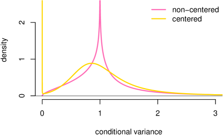
Figure 2: Marginal prior density of a structural shock conditional variance in the two SV models. Source: Lütkepohl et al. (2024).

Both of the SV models share a number of features, such as the flexibility of hierarchical priors with estimated hyper-parameters granting better fit to data and improved forecasting performance, and they facilitate the identification of the structural matrix $\mathbf{B}_{0}$ and shocks through heteroskedasticity following the original ideas by Bertsche and Braun (2022) and Lewis (2021). However, they differ with respect to the features analysed by Lütkepohl et al. (2024) that are presented in Figure 2 plotting the marginal prior distribution of the conditional variances, $\sigma_{n.t}^{2}$, in the two SV models. These densities are implied by the SV model specifications presented in this section. The centred parameterisation concentrate the prior probability mass around point 1 only mildly and goes to infinity when the conditional variance goes to zero. The non-centred parameterisation, on the other hand, concentrates the prior probability mass around point 1 more strongly, goes to zero when the conditional variance goes to zero, and features fat right tail. Finally, in the non-centred parameterisation homoskedasticity can be verified by checking the restriction $\omega_{n}=0$ (see Lütkepohl et al., 2024).

2.2.3 Markov-switching heteroskdasticity

In another heteroskedastic model, the MSH one, the time-variation of the conditional variances is determined by a discrete-valued Markov process $s_{t}$ with $M$ regimes:

$$\sigma_{n.t}^{2}=\sigma_{n.s_{t}}^{2}.$$ (22)

All of the variances switch their values at once according to the latent Markov process takes the values $s_{t}=m\in\{1,\dots,M\}$. The properties of the Markov process itself are determined by the transition matrix $\mathbf{P}$ whose $[\mathbf{P}]_{i.j}$ element denotes the transition probability from regime $i$ to regime $j$ over the next period. The process’ initial probabilities are estimated and denoted by the $M$-vector $\boldsymbol{\pi}_{0}$. In this model used by Brunnermeier et al. (2021), the variances in the $n\textsuperscript{th}$ equation sum to $M$, each of them has the prior expected value equal to 1, and their regimes are given equal prior probabilities of occurrence equal to $M^{-1}$. Therefore, the prior for the conditional variances is the $M$-variate Dirichlet distribution:

$$M^{-1}\left(\sigma_{n.1}^{2},\dots,\sigma_{n.M}^{2}\right)\sim\mathcal{D}irichlet_{M}(\underline{e}_{\sigma},\dots,\underline{e}_{\sigma}),$$ (23)

where the hyper-parameter $\underline{e}_{\sigma}=1$ is fixed. Each of the rows of the transition matrix as well as the initial state probabilities follow the Dirichlet distribution as well:

$$[\mathbf{P}]_{m\cdot} \sim\mathcal{D}irichlet_{M}(\underline{e},\dots,\underline{e})$$ (24)

$$\boldsymbol{\pi}_{0} \sim\mathcal{D}irichlet_{M}(\underline{e}_{0},\dots,\underline{e}_{0}).$$ (25)

The package bsvars offers two alternative models based on MSH. The first is characterised by a stationary Markov process with no absorbing state, and with a positive minimum number of regime occurrences following Droumaguet et al. (2017). In this model, the hyper-parameter $\underline{e}=\underline{e}_{0}$ is fixed to 1 by default and can be modified by the user. The other model represents a novel proposal of a sparse representation that fixes the number of regimes to an over-fitting value $M=20$ (or specified by the user). In this model, many of the regimes will have zero occurrences throughout the sample, which allows the number of regimes with non-zero occurrences to be estimated following the ideas by Malsiner-Walli et al. (2016). Its prior specification is complemented by a hierarchical prior for the hyper-parameter $\underline{e}$:

$$\underline{e}\sim\mathcal{IG}2\left(\underline{s}_{e},\underline{\nu}_{e}\right).$$ (26)

Due to its construction, the sparse MSH model excludes regime-specific interpretation of parameters. Instead, the estimated sequence of conditional variances, $\sigma_{n.t}^{2}$, enjoys standard interpretations. Furthermore, both MSH models provide identification through heteroskedasticity following the ideas by Lanne et al. (2010) and Lütkepohl and Woźniak (2020). The latter paper provides framework for verifying the identification, which in the bsvars package is implemented by verifying the homoskedasticity hypothesis represented by a restriction setting the conditional variances to 1, $\sigma_{n.m}^{2}=1$ for all $m$.

2.3 Models with Non-Normal Shocks

Identification of the structural shocks through non-normality is implemented in the package using the mixture of normal component model (MIX) following the proposal by Lanne and Lütkepohl (2010) and the Student-t distributed shocks as suggested by Lanne et al. (2017).

2.3.1 Mixture of normal components

In this model, the structural shocks follow a conditional $N$-variate normal distribution given the state variable $s_{t}=m\in\{1,\dots,M\}$;

$$u_{t}\mid\mathbf{x}_{t},s_{t}=m,\boldsymbol{\sigma}_{m}^{2}\sim\mathcal{N}_{N}\left(\mathbf{0}_{N},\text{diag}\left(\boldsymbol{\sigma}_{m}^{2}\right)\right),$$ (27)

and where the states are predicted to occur in the next period with probability $\boldsymbol{\pi}_{0}$. The prior specification for these models closely follows that for the MSH models, with the Dirichlet prior for the regime probabilities, $\boldsymbol{\pi}_{0}$, as in (25), and that for the conditionals variances, $\boldsymbol{\sigma}_{m}^{2}$, as in (23).

As long as the predictive state probabilities are constant in these models the classification of the observations into the regimes is performed using filtered and smoothed probabilities, or the posterior realisations of the state allocations $s_{t}$ (see Song and Woźniak, 2021, for a recent review of the methods).

The MIX model comes in two versions as well. The first is the finite mixture model (see e.g. Frühwirth-Schnatter, 2006) in which the number of states, $M$, is fixed and the unconditional state probabilities, $\boldsymbol{\pi}_{0}$, are strictly positive. The latter condition requires non-zero regime occurrences over the sample, a condition that is imposed in the package implementation. An alternative specification is referred to as the sparse mixture model and is based on the proposal by Malsiner-Walli et al. (2016). In this model, the number of the finite mixture components is set to be larger than the real number of the components. Consequently, the number of components with non-zero probability of occurrence is estimated, which is facilitated by allowing the remaining components to have zero occurrences. This sparse structure of normal components implemented thanks to the prior specified for the hyper-parameter $\underline{e}$ of Dirichlet distribution as in equation (26).

The MIX models facilitate the identification through non-normality as proposed by Lanne and Lütkepohl (2010). The hypothesis of normality for a shock, contradicting its identification, is verified by checking whether restriction $\sigma_{n.m}^{2}=1$ holds for all $m$.

2.3.2 Student-t shocks

The Bayesian implementation of the Student-t model follows closely that by Geweke (1993) and is implemented using an inverse gamma scale of normal distribution. Therefore, the conditional normality of the structural shocks from equation (13) is complemented by the marginal prior distributions for variances

$$\sigma_{n.t}^{2}\mid\nu\sim\mathcal{IG}2(\nu-2,\nu).$$ (28)

Such a construction of the structural shock density results in a marginal density for the $n$th shock being a zero-mean, unit-variance Student-t distribution with $\nu>2$ degrees of freedom (see Bauwens et al., 1999)

$$u_{n.t}\mid\mathbf{x}_{t},\nu\sim t\left(0,1,\nu\right).$$ (29)

In this model, the only role of $\sigma_{n.t}^{2}$ is to be integrated out for the sake of specifying the demanded marginal density for the structural shocks.

The prior distribution for the degrees of freedom parameter is set to

$$p(\nu)=\frac{1}{(\nu-1)^{2}}.$$ (30)

This prior density is proper and setting it implies the estimation of the degrees of freedom parameters. Its particular form is further motivated by the fact that it facilitates identification through non-normality verification for a shock by checking the restriction $\nu\rightarrow\infty$ (see also Jensen and Maheu, 2013).

2.4 Hypothesis Verification Using SDDRs

The bsvars package includes unique procedures for the verification of identification and hypotheses on autoregressive parameters. They are based on posterior odds ratio computed using the SDDR by Verdinelli and Wasserman (1995). Consider a general specification of a hypothesis represented by sharp restrictions on the parameters of the model, denoted by $\mathcal{H}_{0}$, and its complement denoted by $\mathcal{H}_{1}$. The SDDR is specified by

$$\frac{\Pr[\mathcal{H}_{0}\mid data]}{\Pr[\mathcal{H}_{1}\mid data]}=SDDR=\frac{p(\mathcal{H}_{0}\mid data)}{p(\mathcal{H}_{0})},$$ (31)

where the LHS equality represents its interpretation as the posterior odds ratio, whereas the RHS equality provides the equivalent form that makes its computation straightforward. Consequently, SDDRs report the ratio of the posterior probability of the restriction to the posterior probability of the unrestricted model. Therefore, a value of the SDDR greater than one provides evidence in favour of the restriction $\mathcal{H}_{0}$, whereas its value less than one provides evidence against this hypothesis, or in favour of $\mathcal{H}_{1}$.

The SDDR computation requires the estimation of the unrestricted model under $\mathcal{H}_{1}$ and the computation of the ratio of the marginal posterior ordinate to the marginal prior ordinate both evaluated at the restriction $\mathcal{H}_{0}$. The specification of the models included in the bsvars package facilitate fast estimation of both ordinates using the estimator proposed by Gelfand and Smith (1990).

2.4.1 Identification verification

In order to verify the identification of structural shocks through time-varying volatility (or non-normality) one needs to verify the hypothesis of homoskedasticity (normality) of individual shocks, which allows them to make probabilistic statements regarding partial or global identification (see Lütkepohl and Woźniak, 2020; Lütkepohl et al., 2024; Lanne et al., 2017). The model is globally identified iff no more than one structural shock is homoskedastic (normal). An individual shock is identified iff it is heteroskedastic (non-normal) or if it is the only homoskedastic (normal) shock in the system.

According to Lütkepohl et al. (2024) the hypothesis of homoskedasticity of the $n$th shock in the non-centred SV model is represented by the restriction

$$\mathcal{H}_{0}:\quad\omega_{n}=0$$ (32)

whereas in the MSH models it given by

$$\mathcal{H}_{0}:\quad\sigma_{n.1}^{2}=\dots\sigma_{n.M}^{2}=1.$$ (33)

The verification of normality of the $n$th shock in the MIX models is performed using the restriction in equation (33), whereas in the Student-t model it is given by

$$\mathcal{H}_{0}:\quad\nu\rightarrow\infty,$$ (34)

as in the limit, the Student-t distribution becomes normal. The model specification makes Bayesian verification of this uncommon restriction straightforward.

2.4.2 Verifying autoregressive specification

Finally, the package makes it possible to verify restrictions on the autoregressive parameters in the form of

$$\mathcal{H}_{0}:\quad\mathbf{S}\text{vec}(\mathbf{A})=\mathbf{r},$$ (35)

where $\text{vec}(\mathbf{A})$ is a vectorised matrix $\mathbf{A}$, $\mathbf{S}$ is an $r\times N(Np+D)$ selection matrix picking $r$ elements of $\mathbf{A}$ to be restricted to the values in the $r$-vector $\mathbf{r}$. Note that the specification of the hierarchical prior leading to the estimated level of autoregressive shrinkage makes the verification of such restrictions less depending on arbitrary choices.

2.5 Posterior Samplers and Computational Details

In this section, we explain bsvars package’s implementation of fast and efficient estimation algorithms obtained thanks to the application of appropriate model specification and frontier econometric techniques best described in Lütkepohl et al. (2024) and Woźniak and Droumaguet (2015).

The objective for choosing the model equations and the prior distributions was to make the estimation using Gibbs sampler technique (see e.g. Casella and George, 1992) and well-specified easy-to-sample-from full conditional posterior distributions. Therefore, the package relies on the reduced form equation (2) for the VAR model. This choice is fairly uncommon in the SVAR literature but it simplifies the estimation of the autoregressive parameters $\mathbf{A}$ directly in the form as they are used for the computations of impulse responses or forecast error variance decomposition. This choice combined with the prior in (3) and specification of the structural form equation (7) facilitates the application of the row-by-row sampler by Chan et al. (2024). As shown by Carriero et al. (2022), relative to the joint estimation of the matrix $\mathbf{A}$ in one step, a usual practice in reduced form VARs, the row-by-row estimation in SVARs can reduce computational complexity of Bayesian estimation from $\mathcal{O}(N^{6})$ to $\mathcal{O}(N^{4})$.

The estimation of the structural form equation (7) is implemented following the quickly converging, efficient, and providing excellent mixing sampling algorithm by Waggoner and Zha (2003a). It offers a flexible framework for setting exclusion restrictions and was also adapted to the SVARs identified through heteroskedasticity and non-normality by Woźniak and Droumaguet (2015). The unique formulation of this equation is particularly convenient for complex heteroskedastic models facilitating the row-by-row estimation of matrix $\mathbf{A}$ and Gibbs sampler for the heteroskedastic process.

The estimation of the Stochastic Volatility models is particularly requiring due to the $N$ independent $T$-valued latent volatility processes estimation that it involves. The implementation of crucial techniques is particularly important here. The sampling algorithms use the 10-component auxiliary mixture technique by Omori et al. (2007) that facilitates the estimation of the log-volatility using the simulation smoother by McCausland et al. (2011) for conditionally Gaussian linear state-space models greatly speeding up the computations (see Woźniak, 2021, for the computational times comparison for various estimation algorithms). Application of appropriate numerical techniques reduces the complexity from $\mathcal{O}(T^{3})$ to $\mathcal{O}(T)$.

Additionally, our specification facilitates the algorithms to estimate heteroskedastic process if the signal from the data is strong, but it also allows them to heavily shrink the posterior towards homoskedasticity, as in equation (14), otherwise. The package implements the adaptation of the ancillarity-sufficiency interweaving strategy that is shown by Kastner and Frühwirth-Schnatter (2014) to improve the efficiency of the sampler when heteroskedasticity is uncertain. Our implementation of the sampling algorithm closely follows the algorithms from package stochvol with adaptations necessary for the SVAR modelling.

The estimation of the Markov switching and mixture models benefits mainly from the implementation of the forward-filtering backward-sampling estimation algorithm for the Markov process $s_{t}$ by Chib (1996) in C++. However, an additional step of choosing the parameterisation of the conditional variances as in equation (23), requiring sampling from a new distribution defined by Woźniak and Droumaguet (2015), assures excellent mixing and sampling efficiency improvements relative to alternative ways of standardising these parameters.

All of the estimation routines for the Markov chain Monte Carlo estimation of the models and those for low level processing of the rich estimation output are implemented based using compiled code in C++. This task is facilitated by the Rcpp package by Eddelbuettel et al. (2011) and Eddelbuettel (2013). The bsvars package relies heavily on linear algebra and pseudo-random number generators. The former is implemented using the package RcppArmadillo by Eddelbuettel and Sanderson (2014) that is a collection of headers linking to the C++ library armadillo by Sanderson and Curtin (2016), as well as on several utility functions for operations on tri-diagonal matrices from package stochvol by Hosszejni and Kastner (2021). The latter refers to the algorithms from the standard normal distribution using package RcppArmadillo, truncated normal distribution RcppTN by Olmsted (2017) implementing the efficient sampler by Robert (1995), and generalised inverse Gaussian distribution using package GIGrvg by Leydold and Hörmann (2017) implementing the sampler by Hörmann and Leydold (2014). All of these developments make the algorithms computationally fast. Still, Bayesian estimation of multivariate dynamic structural models is a requiring task that might take a little while. To give users a better idea of the remaining time the package displays a progress bar implemented using the package RcppProgress by Forner (2020). Finally, the rich structure of the model specification including the prior distributions, identification pattern, and starting values, as well as the rich outputs from the estimation algorithms are organised using dedicated classes within the R6 package by Chang (2021) functionality.

3 Workflows for SVAR analysis

The bsvars package allows the users to design their workflows in several ways. The three main stages include model specification, estimation, and post-estimation analysis.

3.1 The Basic Workflow (also with a Pipe)

The basics of the workflow are presented for the case of a simple homoskedastic SVAR model. Begin by uploading the package and a sample data matrix for the analysis of the US fiscal policy, and setting the seed for the sake of reproducibility:

R> library(bsvars) R> data(us_fiscal_lsuw) R> set.seed(1)

Specify the SVAR model with a lower triangular structural matrix and one autoregressive lag both being the default settings by executing:

R> spec = specify_bsvar$new(us_{f}iscal_{l}suw)\CodeOutput Theidentificationissettothedefaultoptionoflower-triangularstructuralmatrix.\par Theobject\texttt{spec}includesanumberofobjectsthatdefinethemodel,suchasthedatamatrices,fixedhyper-parametersofthepriordistribution,identificationpattern,andstartingvalues.TheestimationofthemodelusingtheMonteCarloMarkovChain(MCMC)methodsisperformedintwosteps.First,theobject\texttt{spec}withmodelspecificationisprovidedtothe\texttt{estimate()}functiontoperform\texttt{1000}iterationsoftheGibbssampler.Thisburn-instageisrunforthealgorithmtoachieveconvergencetothestationaryposteriordistribution.Inthesecondstep,theobject\texttt{burn}isprovidedtothe\texttt{estimate()}functiontoperform\texttt{10000}iterationsoftheGibbssamplerandsavethemintheobject\texttt{post}:\par\CodeChunk\CodeInput R>burn=estimate(spec,1000)R>post=estimate(burn,10000)\par Inthelattercase,thefunction\texttt{estimate()}extractsthelastdrawoftheparametersfromthepreviousrun,usesitasstartingvaluesforthefinalrunoftheestimationalgorithm,andcontinuestheMarkovchainprovidingsamplefromthetargetposteriordistribution.Thiswayofdesigningthe\texttt{estimate()}functionallowstheusertoruntheestimationinseveralsteps,whichisparticularlyusefulforthemodelsrequiringlongerrunsofthesamplingalgorithmtoachieveconvergence.Theusercandiscardthedrawsfromthepreviousstepandcontinuetheestimationinasmanysubsequent\texttt{estimate()}functionrunsasrequired.\par Theposterioroutputisnormalisedwithrespecttothesignsofthestructuralmatrixfollowingtheprocedureby\cite[cite]{\@@bibref{Authors Phrase1YearPhrase2}{WaggonerZha2003norm}{\@@citephrase{(}}{\@@citephrase{)}}}inanautomatedwaybyrunningfunction\texttt{normalise\_posterior()}withintheexecutionofthefunction\texttt{estimate()}.\par Subsequently,usetheestimationoutputtoforecast,say,fourperiodsahead:\par\CodeChunk\CodeInput R>fore=forecast(post,4);summary(fore)\par computeandplotimpulseresponses:\par\CodeChunk\CodeInput R>irfs=compute_{i}mpulse_{r}esponses(post,4);plot(irfs)\par verifywhetherthethirdvariableGrangercausesthefirst:\par\CodeChunk\CodeInput R>H0=matrix(NA,3,4);H0[1,3]=0R>sddr=verify_{a}utoregression(post,H0)R>summary(sddr)\par orperformanyotherpost-estimationanalysis.\par Thesameworkflowcanbecodedusingthe\texttt{\textbar{}\textgreater{}}pipe.Weproposethattheuserbindsthemodelspecificationwiththeestimation:\par\CodeChunk\CodeInput R>set.seed(1)R>us_{f}iscal_{l}suw|>+specify_{b}svar$new()|>+estimate(S=1000)|>+estimate(S=10000)->post\par toobtainexactlythesamedrawsfromtheposteriordistributionasinthepreviousworkflowcollectedinobject\texttt{post}.Thepost-estimationanalysiscanthenbeexecutedby:\par\CodeChunk\CodeInput R>post|>forecast(horizon=4)|>summary()R>post|>compute_{i}mpulse_{r}esponses(horizon=4)|>plot()R>post|>verify_{a}utoregression(hypothesis=H0)|>summary()\par Userpreferences,convenience,andspecificprojectrequirementsshoulddecideontheimplementationoftheprocedureinascript.\par$

3.2 Customizing The Workflow

The package offers a range of models, post-estimation methods, and a set of functions for each of the stages of analysis. The full extent of workflow customization is presented in Figure 3.

Figure 3: Workflow for SVAR analysis

The top of the Figure presents functions to specify the model. Here users can choose a homoskedastic model, one with normal mixture (MIX), Markov-switching heteroskedasticity (MSH), Stochastic Volatility (SV), or t-distributed errors. Then the model can be estimated using the estimate() function repeatedly as long as necessary to obtain $S$ draws from the posterior distribution in the final run. It is recommended then that the user verifies the draws of the $N\times N$ structural matrix contained in an $N\times N\times S$ array post$posterior$B for uni-modality. The lack of thereof may indicate that the automated manner of normalising the posterior draws using function normalise_posterior() was not successful and more work needs to be done here. The default calibration of this algorithm is found to be sufficient for models with exclusion restrictions though.

Given the posterior output, the user can proceed to forecasting, hypotheses verification, or analysis of interpretable quantities. No particular ordering of the operations is recommended and users should implement their competence in the subject matter and consider their project’s requirements here. Forecasting is performed using the forecast() function and includes the possibility of generating conditional predictions given future projections of some of the variables provided in argument conditional_forecast. The user can verify hypotheses about the model parameters using the verify_autoregression() and verify_identification() functions implementing the computation of SDDRs. Finally, the user can compute interpretable quantities such as structural shocks’ conditional standard deviations, fitted values, historical decompositions, impulse responses, MIX and MSH models’ regime probabilities, structural shocks, and forecast error variance decompositions using an appropriate method listed in the last block in Figure 3. The package documentation provides all the necessary details on the arguments and outputs of the functions, which enables further customization of the workflow.

3.3 Generics, Methods, and Functions

Table 1: Summary of package’s generics, methods, and functions

generic or function	first argument class	output class	plot	summary
Specify a model
specify_bsvar	matrix	BSVAR, R6
specify_bsvar_mix	matrix	BSVARMIX, R6
specify_bsvar_msh	matrix	BSVARMSH, R6
specify_bsvar_sv	matrix	BSVARSV, R6
specify_bsvar_t	matrix	BSVART, R6
Estimate a model
estimate	(model classes)	(posterior classes)		✓
	(posterior classes)	(posterior classes)		✓
Normalise posterior output (if necessary)
normalise_posterior	(posterior classes)	(posterior classes)
Forecast
forecast	(posterior classes)	Forecasts	✓	✓
Compute interpretable quantities
compute_conditional_sd	(posterior classes)	PosteriorSigma	✓	✓
compute_fitted_values	(posterior classes)	PosteriorFitted	✓	✓
compute_historical_decompositions	(posterior classes)	PosteriorHD	✓	✓
compute_impulse_responses	(posterior classes)	PosteriorIR	✓	✓
compute_regime_probabilities	(posterior classes)	PosteriorRegimePr	✓	✓
compute_structural_shocks	(posterior classes)	PosteriorShocks	✓	✓
compute_variance_decompositions	(posterior classes)	PosteriorFEVD	✓	✓
Verify hypotheses
verify_autoregression	(posterior classes)	SDDRautoregression		✓
verify_identification	(posterior classes)	(sddr classes)		✓
Classes explanation
(model classes) include BSVAR, BSVARMIX, BSVARMSH, BSVARSV, BSVART
(posterior classes) include PosteriorBSVAR, PosteriorBSVARMIX, PosteriorBSVARMSH, PosteriorBSVARSV, PosteriorBSVART
(sddr classes) include SDDRidSV, SDDRidMIX, SDDRidMSH, SDDRidT

Note: The last two columns indicate availability a dedicated plot or summary method.

The workflows described in this section are possible thanks to a deliberate design of the package’s generics, methods, and functions listed in Table 1. The functions specifying the model are created using the R6 classes to facilitate the management of this complicated object. All the specification details can be adjusted by the user by modifying the elements of the specification object, such as the spec object, that is of a class indicating the specified model, e.g. BSVAR, BSVARSV, … . These objects inherit properties of the list class as well.

All other functions listed in Table 1 define generics that find their particular methods depending on the class of their first argument. Such a construction assures that appropriate estimation algorithm is applied to the model specified by the user. This applies, to all the subsequent stages of the workflow, such as forecasting, hypotheses verification, and computation of interpretable quantities that are performed using the exact algorithms required by the particular specification.

This can be illustrated for the workflow described in the current section. Executing the specification function specify_bsvar$new() creates an object of class BSVAR. Therefore, in the second step the estimate() generic implements method for homoskedastic SVAR model coded in estimate.BSVAR() creating object of class PosteriorBSVAR, which is followed by execution of the method estimate.PosteriorBSVAR() that continues the model estimation using MCMC methods. Consequently, the forecasting is performed using method forecast.PosteriorBSVAR(), impulse responses are computed for this model using method compute_impulse_responses.PosteriorBSVAR(), and the SDDR is estimated using the algorithm dedicated to this particular model using method verify_autoregression.PosteriorBSVAR(). A dedicated set of summary() and plot() methods greatly simplifies the user experience and their workflows.

Finally, generics are designed to be used in other packages with the first implementation in the R package bsvarSIGNs by Wang and Woźniak (2024) providing methods for SVAR models identified with sign, zero, and narrative restrictions.

4 Conclusion

The bsvars package offers fast and efficient algorithms for Bayesian estimation of Structural VARs with a range of specifications for the volatility or distributions of the structural shocks. Thanks to the application of the frontier econometric and numerical techniques the package makes the estimation of multivariate dynamic structural models feasible even for a larger number of variables, complex identification strategies, and non-linear specifications. Its strong reliance on algorithms written in C++ makes it possible to benefit from the best of the two worlds: the convenience of data analysis using R and the computational speed using pre-compiled code written in C++. Finally, the package provides essential generics for applied analyses that facilitate developing coherent workflows for the dependent packages, such as the bsvarSIGNs, package greatly extending the set of models available to the users.

References

- Anderson and Vahid (1998) Anderson HM, Vahid F (1998). “Testing multiple equation systems for common nonlinear components.” Journal of Econometrics, 84(1), 1–36. https://doi.org/10.1016/S0304-4076(97)00076-6.
- Antolín-Díaz and Rubio-Ramírez (2018) Antolín-Díaz J, Rubio-Ramírez JF (2018). “Narrative sign restrictions for SVARs.” 108(10), 2802–2829. 10.1257/aer.20161852.
- Arias et al. (2018) Arias JE, Rubio-Ramírez JF, Waggoner DF (2018). “Inference Based on Structural Vector Autoregressions Identified with Sign and Zero Restrictions: Theory and Applications.” Econometrica, 86(2), 685–720. https://doi.org/10.3982/ECTA14468.
- Bańbura et al. (2010) Bańbura M, Giannone D, Reichlin L (2010). “Large Bayesian Vector Auto Regressions.” Journal of Applied Econometrics, 92, 71– 92. 10.1002/jae.1137.
- Bauwens et al. (1999) Bauwens L, Richard J, Lubrano M (1999). Bayesian inference in dynamic econometric models. Oxford University Press, USA. 10.1093/acprof:oso/9780198773122.001.0001.
- Bernanke et al. (2005) Bernanke BS, Boivin J, Eliasz P (2005). “Measuring the Effects of Monetary Policy: A Factor-Augmented Vector Autoregressive (FAVAR) Approach*.” The Quarterly Journal of Economics, 120(1), 387–422. 10.1162/0033553053327452.
- Bertsche and Braun (2022) Bertsche D, Braun R (2022). “Identification of structural vector autoregressions by stochastic volatility.” Journal of Business & Economic Statistics, 40(1), 328–341. 10.1080/07350015.2020.1813588.
- Boeck et al. (2020) Boeck M, Feldkircher M, Huber F (2020). BGVAR: Bayesian Global Vector Autoregressions. R package version 2.5.7, URL https://CRAN.R-project.org/package=BGVAR.
- Brandt (2006) Brandt PT (2006). \pkgMSBVAR: Bayesian Vector Autoregression Models, Impulse Responses and Forecasting. R package version 0.1.1, URL https://CRAN.R-project.org/package=MSBVAR.
- Brunnermeier et al. (2021) Brunnermeier M, Palia D, Sastry KA, Sims CA (2021). “Feedbacks: Financial Markets and Economic Activity.” American Economic Review, 111(6), 1845–1879. ISSN 0002-8282. 10.1257/aer.20180733.
- Carriero et al. (2022) Carriero A, Chan J, Clark TE, Marcellino M (2022). “Corrigendum to “Large Bayesian vector autoregressions with stochastic volatility and non-conjugate priors” [J. Econometrics 212 (1) (2019) 137–154].” Journal of Econometrics, 227(2), 506–512. https://doi.org/10.1016/j.jeconom.2021.11.010.
- Carriero et al. (2019) Carriero A, Clark TE, Marcellino M (2019). “Large Bayesian vector autoregressions with stochastic volatility and non-conjugate priors.” Journal of Econometrics, 212(1), 137–154. 10.1016/j.jeconom.2019.04.024.
- Casella and George (1992) Casella G, George EI (1992). “Explaining the Gibbs Sampler.” The American Statistician, 46(3), 167–174. 10.1080/00031305.1992.10475878.
- Chan (2020) Chan JC (2020). “Large Bayesian VARs: A flexible Kronecker error covariance structure.” Journal of Business & Economic Statistics, 38(1), 68–79. 10.1080/07350015.2018.1451336.
- Chan and Eisenstat (2018) Chan JC, Eisenstat E (2018). “Bayesian model comparison for time-varying parameter VARs with stochastic volatility.” Journal of Applied Econometrics, 33(4), 509–532. 10.1002/jae.2617.
- Chan et al. (2024) Chan JCC, Koop G, Yu X (2024). “Large Order-Invariant Bayesian VARs with Stochastic Volatility.” Journal of Business & Economic Statistics, 42(2), 825–837. 10.1080/07350015.2023.2252039.
- Chang (2021) Chang W (2021). \pkgR6: Encapsulated Classes with Reference Semantics. R package version 2.5.1, URL https://CRAN.R-project.org/package=R6.
- Chen and Chen (2022) Chen P, Chen C (2022). FAVAR: Bayesian Analysis of a FAVAR Model. R package version 0.1.3, URL https://CRAN.R-project.org/package=FAVAR.
- Chib (1996) Chib S (1996). “Calculating posterior distributions and modal estimates in Markov mixture models.” Journal of Econometrics, 75(1), 79–97. 10.1016/0304-4076(95)01770-4.
- Clark and Ravazzolo (2015) Clark TE, Ravazzolo F (2015). “Macroeconomic Forecasting Performance Under Alternative Specification of Time-Varying Volatility.” Journal of Applied Econometrics, 30, 551–575. 10.1002/jae.2379.
- Danne (2015) Danne C (2015). “\pkgVARsignR: Estimating VARs using sign restrictions in R.” MPRA Paper, 69429, 1–16. URL https://mpra.ub.uni-muenchen.de/68429/.
- Dieppe and van Roye (2024) Dieppe A, van Roye B (2024). The BEAR toolbox. MatLab library version 5.2.1, URL https://github.com/european-central-bank/BEAR-toolbox/.
- Doan et al. (1984) Doan T, Litterman RB, Sims CA (1984). “Forecasting and Conditional Projection Using Realistic Prior Distributions.” Econometric Reviews, 3(June 2013), 37–41. 10.1080/07474938408800053.
- Droumaguet et al. (2017) Droumaguet M, Warne A, Woźniak T (2017). “Granger Causality and Regime Inference in Markov Switching VAR Models with Bayesian Methods.” Journal of Applied Econometrics, 32(4), 802–818. 10.1002/jae.2531.
- Dynare Team (2024) Dynare Team (2024). Dynare: Reference Manual, Release 6.1. URL https://www.dynare.org/.
- Eddelbuettel (2013) Eddelbuettel D (2013). Seamless R and C++ Integration with \pkgRcpp. Springer, New York, NY. 10.1007/978-1-4614-6868-4.
- Eddelbuettel et al. (2011) Eddelbuettel D, François R, Allaire J, Ushey K, Kou Q, Russel N, Chambers J, Bates D (2011). “\pkgRcpp: Seamless R and C++ integration.” Journal of Statistical Software, 40(8), 1–18. 10.18637/jss.v040.i08.
- Eddelbuettel and Sanderson (2014) Eddelbuettel D, Sanderson C (2014). “\pkgRcppArmadillo: Accelerating R with high-performance C++ linear algebra.” Computational Statistics & Data Analysis, 71, 1054–1063. 10.1016/j.csda.2013.02.005.
- Forner (2020) Forner K (2020). \pkgRcppProgress: An Interruptible Progress Bar with OpenMP Support for C++ in R Packages. R package version 0.4.2, URL https://CRAN.R-project.org/package=RcppProgress.
- Frühwirth-Schnatter (2006) Frühwirth-Schnatter S (2006). Finite Mixture and Markov Switching Models. Springer. 10.1007/978-0-387-35768-3.
- Fry and Pagan (2011) Fry R, Pagan A (2011). “Sign restrictions in structural vector autoregressions: A critical review.” Journal of Economic Literature, 49(4), 938–60. 10.1257/jel.49.4.938.
- Gelfand and Smith (1990) Gelfand AE, Smith AFM (1990). “Sampling-Based Approaches to Calculating Marginal Densities.” Journal of the American Statistical Association, 85(410), 398–409. 10.1080/01621459.1990.10476213.
- Geweke (1993) Geweke J (1993). “Bayesian treatment of the independent student-t linear model.” Journal of Applied Econometrics, 8(S1), S19–S40. 10.1002/jae.3950080504.
- Giannone et al. (2015) Giannone D, Lenza M, Primiceri GE (2015). “Prior selection for Vector Autoregressions.” Review of Economics and Statistics, 97(2), 436–451. 10.1162/REST_a_00483.
- Gruber (2024) Gruber L (2024). bayesianVARs: MCMC Estimation of Bayesian Vectorautoregressions. R package version 0.1.3, URL https://CRAN.R-project.org/package=bayesianVARs.
- Hörmann and Leydold (2014) Hörmann W, Leydold J (2014). “Generating generalized inverse Gaussian random variates.” Statistics and Computing, 24(4), 547–557. 10.1007/s11222-013-9387-3.
- Hosszejni and Kastner (2021) Hosszejni D, Kastner G (2021). “Modeling Univariate and Multivariate Stochastic Volatility in R with \pkgstochvol and \pkgfactorstochvol.” Journal of Statistical Software, 100(12). 10.18637/jss.v100.i12.
- Jensen and Maheu (2013) Jensen MJ, Maheu JM (2013). “Bayesian semiparametric multivariate GARCH modeling.” Journal of Econometrics, 176(1), 3–17. 10.1016/j.jeconom.2013.03.009.
- Kalliovirta et al. (2016) Kalliovirta L, Meitz M, Saikkonen P (2016). “Gaussian mixture vector autoregression.” Journal of Econometrics, 192(2), 485–498. 10.1016/j.jeconom.2016.02.012.
- Kastner and Frühwirth-Schnatter (2014) Kastner G, Frühwirth-Schnatter S (2014). “Ancillarity-sufficiency interweaving strategy (ASIS) for boosting MCMC estimation of stochastic volatility models.” Computational Statistics & Data Analysis, 76, 408 – 423. https://doi.org/10.1016/j.csda.2013.01.002.
- Kilian and Lütkepohl (2017) Kilian L, Lütkepohl H (2017). Structural Vector Autoregressive Analysis. Cambridge University Press, Cambridge. 10.1017/9781108164818.
- Krueger (2015) Krueger F (2015). \pkgbvarsv: Bayesian Analysis of a Vector Autoregressive Model with Stochastic Volatility and Time-Varying Parameters. R package version 1.1, URL https://CRAN.R-project.org/package=bvarsv.
- Kuschnig and Vashold (2021) Kuschnig N, Vashold L (2021). “\pkgBVAR: Bayesian Vector Autoregressions with Hierarchical Prior Selection in R.” Journal of Statistical Software, 100(14), 1–27. 10.18637/jss.v100.i14.
- Lange et al. (2021) Lange A, Dalheimer B, Herwartz H, Maxand S (2021). “\pkgsvars: An R Package for Data-Driven Identification in Multivariate Time Series Analysis.” Journal of Statistical Software, 97(5), 1–34. 10.18637/jss.v097.i05.
- Lanne and Lütkepohl (2010) Lanne M, Lütkepohl H (2010). “Structural Vector Autoregressions With Nonnormal Residuals.” Journal of Business & Economic Statistics, 28(1), 159–168. 10.1198/jbes.2009.06003.
- Lanne et al. (2010) Lanne M, Lütkepohl H, Maciejowska K (2010). “Structural vector autoregressions with Markov switching.” Journal of Economic Dynamics and Control, 34, 121–131. 10.1016/j.jedc.2009.08.002.
- Lanne et al. (2017) Lanne M, Meitz M, Saikkonen P (2017). “Identification and estimation of non-Gaussian structural vector autoregressions.” Journal of Econometrics, 196(2), 288–304. 10.1016/j.jeconom.2016.06.002.
- Lee and Kim (2019) Lee N, Kim SH (2019). VARshrink: Shrinkage Estimation Methods for Vector Autoregressive Models. R package version 0.3.1, URL https://CRAN.R-project.org/package=VARshrink.
- Lewis (2021) Lewis DJ (2021). “Identifying Shocks via Time-Varying Volatility.” The Review of Economic Studies, 88(6), 3086–3124. 10.1093/restud/rdab009.
- Leydold and Hörmann (2017) Leydold J, Hörmann W (2017). \pkgGIGrvg: Random Variate Generator for the GIG Distribution. R package version 0.5, URL https://CRAN.R-project.org/package=GIGrvg.
- Lütkepohl et al. (2024) Lütkepohl H, Shang F, Uzeda L, Woźniak T (2024). “Partial Identification of Heteroskedastic Structural VARs: Theory and Bayesian Inference.” Working paper, University of Melbourne. 10.48550/arXiv.2404.11057.
- Lütkepohl and Woźniak (2020) Lütkepohl H, Woźniak T (2020). “Bayesian inference for structural vector autoregressions identified by Markov-switching heteroskedasticity.” Journal of Economic Dynamics and Control, 113, 103862. 10.1016/j.jedc.2020.103862.
- Lütkepohl and Netšunajev (2017) Lütkepohl H, Netšunajev A (2017). “Structural vector autoregressions with smooth transition in variances.” Journal of Economic Dynamics and Control, 84, 43–57. https://doi.org/10.1016/j.jedc.2017.09.001.
- Malsiner-Walli et al. (2016) Malsiner-Walli G, Frühwirth-Schnatter S, Grün B (2016). “Model-based clustering based on sparse finite Gaussian mixtures.” Statistics and computing, 26(1), 303–324. 10.1007/s11222-014-9500-2.
- McCausland et al. (2011) McCausland WJ, Miller S, Pelletier D (2011). “Simulation smoothing for state–space models: A computational efficiency analysis.” Computational Statistics & Data Analysis, 55(1), 199–212. 10.1016/j.csda.2010.07.009.
- Mohr (2022) Mohr FX (2022). \pkgbvartools: Bayesian Inference of Vector Autoregressive and Error Correction Models. R package version 0.2.1, URL https://CRAN.R-project.org/package=bvartools.
- Nicholson et al. (2023) Nicholson W, Matteson D, Bien J, Wilms I (2023). BigVAR: Dimension Reduction Methods for Multivariate Time Series. R package version 1.1.2, URL https://CRAN.R-project.org/package=BigVAR.
- Olmsted (2017) Olmsted J (2017). \pkgRcppTN: Rcpp-Based Truncated Normal Distribution RNG and Family. R package version 0.2-2, URL https://CRAN.R-project.org/package=RcppTN.
- Omori et al. (2007) Omori Y, Chib S, Shephard N, Nakajima J (2007). “Stochastic Volatility with Leverage: Fast and Efficient Likelihood Inference.” Journal of Econometrics, 140(2), 425–449. 10.1016/j.jeconom.2006.07.008.
- Pfaff (2008) Pfaff B (2008). “VAR, SVAR and SVEC Models: Implementation Within R Package \pkgvars.” Journal of Statistical Software, 27(4), 1–32. 10.18637/jss.v027.i04.
- Primiceri (2005) Primiceri GE (2005). “Time Varying Structural Vector Autoregressions and Monetary Policy.” The Review of Economic Studies, 72(3), 821–852. 10.1111/j.1467-937X.2005.00353.x.
- R Core Team (2021) R Core Team (2021). R: A Language and Environment for Statistical Computing. R Foundation for Statistical Computing, Vienna, Austria. URL https://www.R-project.org/.
- Rigobon (2003) Rigobon R (2003). “Identification through heteroskedasticity.” Review of Economics and Statistics, 85, 777–792. https://doi.org/10.1162/003465303772815727.
- Robert (1995) Robert CP (1995). “Simulation of truncated normal variables.” Statistics and Computing, 5(2), 121–125. 10.1007/BF00143942.
- Rubio-Ramirez et al. (2010) Rubio-Ramirez JF, Waggoner DF, Zha T (2010). “Structural vector autoregressions: Theory of identification and algorithms for inference.” The Review of Economic Studies, 77(2), 665–696. 10.1111/j.1467-937X.2009.00578.x.
- Sanderson and Curtin (2016) Sanderson C, Curtin R (2016). “\pkgArmadillo: a template-based C++ library for linear algebra.” Journal of Open Source Software, 1(2), 26. 10.21105/joss.00026.
- Sims (1980) Sims CA (1980). “Macroeconomics and reality.” Econometrica, 48(1), 1–48. 10.2307/1912017.
- Sims and Zha (2006) Sims CA, Zha T (2006). “Were There Regime Switches in U.S. Monetary Policy?” American Economic Review, 96(1), 54–81. 10.1257/000282806776157678.
- Song and Woźniak (2021) Song Y, Woźniak T (2021). “Markov Switching.” In Oxford Research Encyclopedia of Economics and Finance. 10.1093/acrefore/9780190625979.013.174.
- Tsay et al. (2022) Tsay RS, Wood D, Lachmann J (2022). \pkgMTS: All-Purpose Toolkit for Analyzing Multivariate Time Series (MTS) and Estimating Multivariate Volatility Models. R package version 1.2.1, URL http://CRAN.R-project.org/package=MTS.
- Uhlig (2005) Uhlig H (2005). “What are the effects of monetary policy on output? Results from an agnostic identification procedure.” Journal of Monetary Economics, 52(2), 381–419. 10.1016/j.jmoneco.2004.05.007.
- Verdinelli and Wasserman (1995) Verdinelli I, Wasserman L (1995). “Computing Bayes Factors Using a Generalization of the Savage-Dickey Density Ratio.” Journal of the American Statistical Association, 90(430), 614–618. 10.1080/01621459.1995.10476554.
- Virolainen (2024a) Virolainen S (2024a). gmvarkit: Estimate Gaussian and Student’s t Mixture Vector Autoregressive Models. R package version 2.1.2, URL https://CRAN.R-project.org/package=gmvarkit.
- Virolainen (2024b) Virolainen S (2024b). “Identification by non-Gaussianity in structural threshold and smooth transition vector autoregressive models.” 10.48550/arXiv.2404.19707. 2404.19707.
- Virolainen (2024c) Virolainen S (2024c). sstvars: Toolkit for Reduced Form and Structural Smooth Transition Vector Autoregressive Models. R package version 1.0.1, URL https://CRAN.R-project.org/package=sstvars.
- Virolainen (2024d) Virolainen S (2024d). “A Statistically Identified Structural Vector Autoregression with Endogenously Switching Volatility Regime.” Journal of Business & Economic Statistics, 0(0), 1–20. 10.1080/07350015.2024.2322090.
- Waggoner and Zha (2003a) Waggoner DF, Zha T (2003a). “A Gibbs sampler for structural vector autoregressions.” Journal of Economic Dynamics and Control, 28(2), 349–366. 10.1016/S0165-1889(02)00168-9.
- Waggoner and Zha (2003b) Waggoner DF, Zha T (2003b). “Likelihood preserving normalization in multiple equation models.” Journal of Econometrics, 114(2), 329–347. https://doi.org/10.1016/S0304-4076(03)00087-3.
- Wang and Woźniak (2024) Wang X, Woźniak T (2024). \pkgbsvarSIGNs: Bayesian SVARs with Sign, Zero, and Narrative Restrictions. R package version 1.0, URL https://CRAN.R-project.org/package=bsvarSIGNs.
- Wilms et al. (2023) Wilms I, Matteson DS, Bien J, Basu S, Nicholson W, Wegner E (2023). bigtime: Sparse Estimation of Large Time Series Models. R package version 0.2.3, URL https://CRAN.R-project.org/package=bigtime.
- Woźniak (2016) Woźniak T (2016). “Bayesian Vector Autoregressions.” Australian Economic Review, 49(3), 365–380. 10.1111/1467-8462.12179.
- Woźniak (2021) Woźniak T (2021). “Simulation Smoother using \pkgRcppArmadillo.” RcppGallery, URL: https://gallery.rcpp.org/articles/simulation-smoother-using-rcpparmadillo/, (Accessed on 5 September 2021).
- Woźniak (2024) Woźniak T (2024). \pkgbsvars: Bayesian Estimation of Structural Vector Autoregressive Models. R package version 3.2, URL http://CRAN.R-project.org/package=bsvars.
- Woźniak and Droumaguet (2015) Woźniak T, Droumaguet M (2015). “Assessing Monetary Policy Models: Bayesian Inference for Heteroskedastic Structural VARs.” University of Melbourne Working Papers Series, 2017. 10.13140/RG.2.2.19492.55687.