Spatial-Mamba: Effective Visual State Space
Models via Structure-aware State Fusion

Abstract

Selective state space models (SSMs), such as Mamba (Gu & Dao, 2023), highly excel at capturing long-range dependencies in 1D sequential data, while their applications to 2D vision tasks still face challenges. Current visual SSMs often convert images into 1D sequences and employ various scanning patterns to incorporate local spatial dependencies. However, these methods are limited in effectively capturing the complex image spatial structures and the increased computational cost caused by the lengthened scanning paths. To address these limitations, we propose Spatial-Mamba, a novel approach that establishes neighborhood connectivity directly in the state space. Instead of relying solely on sequential state transitions, we introduce a structure-aware state fusion equation, which leverages dilated convolutions to capture image spatial structural dependencies, significantly enhancing the flow of visual contextual information. Spatial-Mamba proceeds in three stages: initial state computation in a unidirectional scan, spatial context acquisition through structure-aware state fusion, and final state computation using the observation equation. Our theoretical analysis shows that Spatial-Mamba unifies the original Mamba and linear attention under the same matrix multiplication framework, providing a deeper understanding of our method. Experimental results demonstrate that Spatial-Mamba, even with a single scan, attains or surpasses the state-of-the-art SSM-based models in image classification, detection and segmentation. Source codes and trained models can be found at https://github.com/EdwardChasel/Spatial-Mamba.

1 Introduction

State space models (SSMs) are powerful tools for analyzing dynamic systems with hidden states, and they have long been utilized in fields like control theory, signal processing, and economics (Friston et al., 2003; Hafner et al., 2019; Gu et al., 2020). SSMs have been recently introduced into deep learning (Gu et al., 2021a), especially in natural language processing (NLP) (Gu & Dao, 2023), thanks to their use of specially parameterized matrices. A major advancement is the introduction of selective mechanisms and hardware-aware optimizations for parallel computing, as demonstrated by Mamba (Gu & Dao, 2023), which selectively retains or discards information based on the relevance of each element in a sequence, efficiently modeling long-distance dependencies with linear complexity.

The significant success of Mamba in NLP inspires researchers to investigate how SSMs can be applied to visual tasks. Unlike 1D sequences, visual data are typically characterized by 2D spatial structures. Therefore, it is crucial to maintain the spatial dependencies within images while adapting the information selection and propagation mechanisms in Mamba. Existing visual SSMs (Zhu et al., 2024; Liu et al., 2024; Yang et al., 2024; Huang et al., 2024; He et al., 2024a; Xiao et al., 2024) often use some scanning strategies to flatten 2D visual data into several 1D sequences from different directions, and then process the flattened 1D sequences using the original Mamba. These scanning strategies can be broadly categorized into three types: sweeping scan, continuous scan and local scan, as shown in Figs. 1(a)-1(c), respectively.

Vim (Zhu et al., 2024) and VMamba (Liu et al., 2024) employ sweeping bidirectional scan and four-way scan, which are illustrated in Fig. 1(a). These strategies aim to reduce spatial direction sensitivity and adapt the network architecture for visual tasks. Yang et al. (2024) argued that sweeping scans neglect the importance of spatial continuity, and they introduced a continuous scanning order, as shown in Fig. 1(b), to better integrate the inductive biases from visual data. Huang et al. (2024) argued that scanning the entire image may not effectively capture local spatial relationships. Instead, they presented LocalMamba by using several local scanning modes, as shown in Fig. 1(c), which divides an image into distinct windows to capture local dependencies. Beyond the above mentioned scanning patterns, other scanning methods such as Hilbert scanning (He et al., 2024a) and dynamic tree scanning (Xiao et al., 2024) have also been proposed to adapt SSMs to visual tasks.

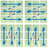
(a) Sweeping Scan

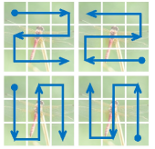
(b) Continuous Scan

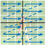
(c) Local Scan

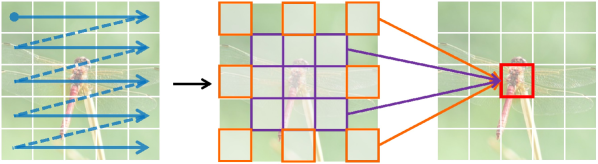
(d) Structure-aware state fusion with unidirectional scan

Figure 1: Illustration of the scanning patterns of existing visual SSMs (from sub-figures (a) to (c)) and our proposed Spatial-Mamba with structure-aware state fusion (sub-figure (d)).

While the existing scanning strategies partially address the issue of aligning spatial structures with sequential SSMs, they are limited in model effectiveness and efficiency. On one hand, directional scanning inevitably alters the spatial relationships between pixels, disrupting the inherent spatial context in an image. For example, in the sweeping scan (Fig. 1(a)), the distance between a pixel and its left or right neighbor is 1, while its distance to the top or bottom neighbor equals to the image width. This distortion can hinder the models to understand the spatial relationships in the original visual data. On the other hand, the fixed scanning paths, such as the commonly used four-directional scan (Figs. 1(a) and  1(b)), are not effective enough to capture the complex and varying spatial relationships in an image, while introducing more scanning directions would also result in excessive computations. Therefore, it is imperative to explore how to design more effective and structure-aware SSMs for visual tasks.

To achieve this goal, we make an important attempt in this paper and present Spatial-Mamba, which is designed to capture the spatial dependencies of neighboring features in the latent state space. The processing flow of Spatial-Mamba consists of three stages. First, as shown in the left of Fig. 1(d), visual data are converted into sequential data using unidirectional sweeping scan. The state variables are computed based on the state transition equations of the original SSMs and then reshaped back into the visual format. Second, the state variables are processed through a structure-aware state fusion (SASF) equation, which employs dilated convolutions to re-weight and merge nearby state variables, as shown in the left of Fig. 1(d). Finally, these structure-aware state variables are fed into the observation equation to produce the final output variables. The SASF equation not only enables efficient skip connections between non-sequential elements in sequences but also enhances the model ability to capture spatial relationships, leading to more accurate representations of the underlying visual structure. Furthermore, we show that Spatial-Mamba, original Mamba and linear attention can all be represented under the same framework using structured matrices, which offers a more coherent understanding of our proposed method. We validate the superiority of Spatial-Mamba across fundamental vision tasks such as image classification, detection, and segmentation. The results demonstrate that Spatial-Mamba, even with a single scan, achieves or surpasses the performance of recent state-of-the-arts using different scanning strategies.

2 Related Work

State space models (SSMs). Gu et al. (2021b) firstly introduced the linear state space layer (LSSL) into the HiPPO framework (Gu et al., 2020) to efficiently handle the long-range dependencies in long sequences. Gu et al. (2021a) then significantly improved the efficiency of SSMs by representing the parameters as diagonal plus low-rank matrix. The so-called S4 model triggers a wave of structured SSMs (Smith et al., 2022; Fu et al., 2022; Gupta et al., 2022; Gu & Dao, 2023). Smith et al. (2022) proposed S5 by introducing parallel scans to S4 layer while maintaining the computational efficiency of S4. Recently, Gu & Dao (2023) developed Mamba, which incorporates a data-dependent selection mechanism into S4 layer and simplifies the computation and architecture in a hardware-friendly way, achieving Transformer-like modeling capability with linear complexity. Building on that, Dao & Gu (2024) presented Mamba2, which reveals the connections between SSMs and attention with specific structured matrix. This framework simplifies the parameter matrix to a scalar representation, making it feasible to explore larger and more expressive state spaces without sacrificing efficiency.

Visual SSMs. Although traditional SSMs perform well in processing NLP sequential data and capturing temporal dependencies, they struggle in handling multi-dimensional spatial structure inherent in visual data. This limitation poses a challenge for developing effective visual SSMs. S4ND (Nguyen et al., 2022) is among the first SSM-based models for multi-dimensional data, which separates each dimension with an independent 1D SSM. Baron et al. (2023) generalized S4ND as a discrete multi-axial system and proposed the 2D-SSM spatial layer, successfully extending the 1D SSMs to 2D SSMs. More recent visual SSMs prefer to design multiple scanning orders or patterns to maintain the spatial consistency, including bidirectional (Liu et al., 2024), four-way (Zhu et al., 2024), continuous (Yang et al., 2024), zigzag (Hu et al., 2024), window-based (Huang et al., 2024), and topology-based scanning (He et al., 2024a; Xiao et al., 2024). These visual SSMs have been used in multimodal foundation models (Qiao et al., 2024; Mo & Tian, 2024), image restoration (Guo et al., 2024; Shi et al., 2024), medical image analysis (Yue & Li, 2024; Ma et al., 2024; He et al., 2024b; Liao et al., 2024) and other visual tasks (Chen et al., 2024; Li et al., 2024; Yao et al., 2024), demonstrating the potential of SSMs in visual data understanding.

3 Preliminaries

SSMs are commonly used for analyzing sequential data and modeling continuous linear time-invariant (LTI) systems (Williams & Lawrence, 2007). An input sequence $\displaystyle u(t)\in\mathbb{R}$ is transformed into an output sequence $\displaystyle y(t)\in\mathbb{R}$ through a state variable $\displaystyle x(t)\in\mathbb{C}^{N}$. Here, $t>0$ represents the time index, and $N$ indicates the dimension of the state variable. This dynamic system can be described by the linear state transition and observation equations (Kalman, 1960): $\displaystyle x^{\prime}(t)={\bm{A}}x(t)+{\bm{B}}u(t),y(t)={\bm{C}}x(t)+{\bm{D}}u(t)$, where $\displaystyle{\bm{A}}\in\mathbb{C}^{N\times N}$ is the state transition matrix, $\displaystyle{\bm{B}}$, $\displaystyle{\bm{C}}\in\mathbb{C}^{N}$ and $\displaystyle{\bm{D}}\in\mathbb{C}^{1}$ control the dynamics of the system. The state transition and observation equations describe how the system evolves over time and how the state variables relate to the observed outputs.

To effectively integrate continuous-time SSMs into the deep learning framework, it is essential to discretize the continuous-time models. One commonly employed technique is the Zero-Order Hold (ZOH) discretization (Gu & Dao, 2023). The ZOH method approximates the continuous-time system by holding the input constant over each discrete time interval. Specifically, given a timescale $\mathbf{\Delta}$, which represents the interval between discrete time steps, and defining $\overline{{\bm{A}}}$ and $\overline{{\bm{B}}}$ as discrete parameters, the ZOH rule is applied as $\displaystyle\overline{{\bm{A}}}=e^{\mathbf{\Delta}{\bm{A}}}$ and $\overline{{\bm{B}}}=(\mathbf{\Delta}{\bm{A}})^{-1}(e^{\mathbf{\Delta}{\bm{A}}}-I)\mathbf{\Delta}{\bm{B}}$.

However, real-world processes often change over time and cannot be accurately described by a LTI system. As highlighted in Mamba (Gu & Dao, 2023), time-varying systems can focus more on relevant information and offer a more accurate and realistic representation of dynamic systems. In Mamba, the parameters of the SSMs are made context-aware and adaptive through selective functions. This is achieved by modifying the parameters $\mathbf{\Delta},{\bm{B}},{\bm{C}}$ as simple functions of the input sequence $u_{t}$, resulting in input-dependent parameters $\mathbf{\Delta}_{t}=s_{\Delta}(u_{t}),{\bm{B}}_{t}=s_{B}(u_{t})$ and ${\bm{C}}_{t}=s_{C}(u_{t})$. Then the input-dependent discrete parameters $\overline{{\bm{A}}}_{t}$ and $\overline{{\bm{B}}}_{t}$ can be calculated accordingly. Consequently, the discrete state transition and observation equations can be calculated as follows:

$$x_{t}=\overline{{\bm{A}}}_{t}x_{t-1}+\overline{{\bm{B}}}_{t}u_{t},\quad y_{t}={\bm{C}}_{t}x_{t}+{\bm{D}}u_{t}.$$ (1)

A simplified illustration of the above process is shown in Fig. 2(a).

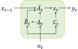
(a) SSM in Mamba

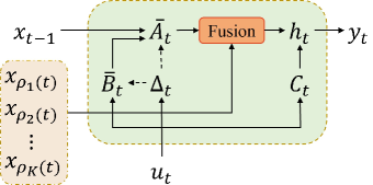
(b) SSM in Spatial-Mamba

Figure 2: Illustrations of the SSM in (a) Mamba and (b) our Spatial-Mamba, where the residual term $\displaystyle{\bm{D}}$ is omitted. In (b), ‘Fusion’ refers to our proposed structure-aware state fusion (SASF) equation.

(a) Input

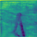
(b) Original state $x_{t}$

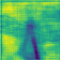
(c) Fused state $h_{t}$

(d) Original state $x_{t}$

(e) Fused state $h_{t}$

Figure 3: Visualization of state variables before and after applying the SASF equation. Sub-figures (b) and (c) show the mean of state variables across all channels in the first layer of Spatial-Mamba, while sub-figures (d) and (e) display the state variables for a specific channel in the last layer.

4 Spatial-Mamba

4.1 Formulation of Spatial-Mamba

Spatial-Mamba is designed to capture the spatial dependencies of neighboring features in the latent state space. To achieve this goal, different from previous methods (Zhu et al., 2024; Liu et al., 2024; Huang et al., 2024) that commonly employ multiple scanning directions, we introduce a new structure-aware state fusion (SASF) equation into the original Mamba formulas (refer to Eq. (1)). The entire process of Spatial-Mamba can be described by three equations: the state transition equation, the SASF and the observation equation, which are formulated as:

$$x_{t}=\overline{{\bm{A}}}_{t}x_{t-1}+\overline{{\bm{B}}}_{t}u_{t},\quad h_{t}=\sum_{k\in\Omega}\alpha_{k}x_{\rho_{k}(t)},\quad y_{t}={\bm{C}}_{t}h_{t}+{\bm{D}}u_{t},$$ (2)

where $x_{t}$ is the original state variable, $h_{t}$ is the structure-aware state variable, $\Omega$ is the neighbor set, and $\rho_{k}(t)$ is the index of the $k$-th neighbor of position $t$. Fig. 2(b) illustrates the SSM flow in the proposed Spatial-Mamba. Compared with the original Mamba in Fig. 2(a), we can see that the original state variable $x_{t}$ is directly influenced by its previous state $x_{t-1}$, while the structure-aware state variable $h_{t}$ incorporates additional neighboring state variables $x_{\rho_{1}(t)},x_{\rho_{2}(t)},\dots,x_{\rho_{K}(t)}$ through a fusion mechanism, where $K=|\Omega|$ denotes the size of neighbor set. By considering both temporal and spatial information, the fused state variable $h_{t}$ gains a richer context, leading to improved adaptability and a more comprehensive understanding of the image.

The proposed Spatial-Mamba can be implemented in three steps. As shown in Fig. 1(d), the input image is first flattened into a 1D sequence $u_{t}$, with which the state $x_{t}$ is computed using the state transition equation $x_{t}=\overline{{\bm{A}}}_{t}x_{t-1}+\overline{{\bm{B}}}_{t}u_{t}$. The computed states are then reshaped back into the 2D format. To enable each state to be aware of its neighboring states in the 2D space, we introduce the SASF equation $h_{t}=\sum_{k\in\Omega}\alpha_{k}x_{\rho_{k}(t)}$. For a state variable $x_{t}$, we apply linear weighting to its neighboring states $\rho_{k}(t)$ in the neighborhood $\Omega$ using weights $\alpha_{k}$ so that we can effectively integrate local dependency information into a new state $h_{t}$, resulting in a more contextually informative representation. Finally, the output is generated from this enriched state $h_{t}$ through the observation equation $y_{t}={\bm{C}}_{t}h_{t}+{\bm{D}}u_{t}$. This SASF approach helps the model to incorporate the local structural information in visual learning while retaining the benefits of original Mamba.

In practice, we simply employ multi-scale dilated convolutions (Yu, 2015) to linearly weight adjacent state variables, enhancing spatial relationship characterizations and enabling skip connections. Specifically, we use three $3\times 3$ depth-wise filters with dilation factors $d=1,3,5$ to construct the neighbor set $\Omega_{d}=\{(i,j)|i,j\in\{-d,0,d\}\}$. The SASF equation in Eq. (2) can be rewritten as:

$$h_{t}=\sum_{d=1,3,5}\sum_{i,j\in\Omega_{d}}k_{ij}^{d}\cdot x_{t+iw+j},$$ (3)

where $k_{ij}^{d}$ represents the filter weight for dilation factor $d$ at position $(i,j)$, $x_{t+iw+j}$ denotes the neighbor of the state $x_{t}$ located at the position $(i,j)$, and $w$ indicates the width of the image.

To gain an intuitive understanding of SASF, we visualize the original state variables and our proposed structure-aware state variables in Fig. 3. One can see that the original state $x_{t}$ (Fig. 3(b)) struggles to differentiate between the foreground and background. In contrast, the structure-aware state $h_{t}$ (Fig. 3(c)), which has been refined through a SASF process, effectively separates these regions. Moreover, the original state variable $x_{t}$ in Fig. 3(d) only shows horizontal attenuation along the scanning direction (gradually darkening from the brightest value in the upper left corner), while the fused state variable $h_{t}$ in Fig. 3(e) demonstrates decay along the horizontal, vertical and diagonal directions. This improvement stems from its ability to leverage spatial relationships within the image, leading to a more accurate and context-aware representation.

4.2 Network Architecture

The overall architecture of Spatial-Mamba is depicted in Fig. 4. It consists of four successive stages, resembling the structure of Swin-Transformer (Liu et al., 2021). We introduce three variants of Spatial-Mamba model at different scales: Spatial-Mamba-T (tiny), Spatial-Mamba-S (small), and Spatial-Mamba-B (base). The detailed configurations are provided in Appendix A. Specifically, an input image $I\in\mathbb{R}^{H\times W\times 3}$ is first processed by an overlapped stem layer to generate a 2D feature map with dimension of $\frac{H}{4}\times\frac{W}{4}\times C$. This feature map is then fed into four successive stages. Each stage comprises multiple Spatial-Mamba blocks, followed by a down-sampling layer with a factor of 2 (except for the last stage), resulting in hierarchical features. Finally, a head layer is employed to process these features to produce corresponding image representations for specific downstream tasks.

The Spatial-Mamba block forms the fundamental building unit of our architecture, which consists of a Structure-aware SSM and a Feed-Forward Network (FFN) with skip connections, as illustrated in the bottom left of Fig. 4. Building upon the Mamba block design (Gu & Dao, 2023), the Structure-aware SSM, illustrated in the bottom right of Fig. 4, is implemented by substituting the original 1D causal convolution with a $3\times 3$ depth-wise convolution and replacing the original S6 module with our proposed SASF module, achieving local neighborhood connectivity in state spaces with linear complexity. Moreover, a local perception unit (LPU) (Guo et al., 2022) is employed before the Spatial-Mamba block and FFN to extract local information inside image patches.

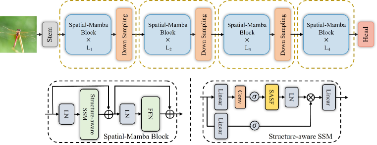
Figure 4: Overall network architecture of Spatial-Mamba.

4.3 Connection with Original Mamba and Linear Attention

We analyze in-depth the similarities and disparities among linear attention (Katharopoulos et al., 2020), original Mamba (Gu & Dao, 2023) and our Spatial-Mamba, providing a better understanding of the working mechanism of our proposed method. Detailed derivations are provided in Appendix B.

Linear attention is an improved self-attention (SA) mechanism, reducing the computational complexity of SA to linear by using a kernel function $\phi$. For an input sequence $u_{t}$, the query $q_{t}$, key $k_{t}$, and value $v_{t}$ are computed by projecting $u_{t}$ with different weight matrices. In autoregressive models, to prevent the model from attending to future tokens, the $t$-th query is restricted by the previous keys, i.e., $k_{s},s\leq t$. Thus, if the kernel function $\phi$ is an identity map, the calculation of single head linear attention without normalization can be formulated as: $y_{t}=\sum_{s\leq t}q_{t}(k_{s}^{T}v_{s})$. Letting $x_{t}=\sum_{s\leq t}k_{s}^{T}v_{s}$, then we have $x_{t}=x_{t-1}+k_{t}^{T}v_{t}$. The linear attention can be rewritten as $y_{t}=q_{t}x_{t}$. This reveals that linear attention is actually a special case of linear recursion. The hidden state variable $x_{t}$ is updated by the outer-product $k_{s}^{T}v_{s}$, and the final output $y_{t}$ is observed by multiplying $x_{t}$ with the query $q_{t}$. If we define ${\bm{C}}_{t}=q_{t}$ and $\overline{{\bm{B}}}_{s}=k_{s}^{T}$, the linear attention can be expressed in a form similar to that of SSM:

$$y_{t}=\sum_{s\leq t}{\bm{C}}_{t}\overline{{\bm{B}}}_{s}v_{s},$$ (4)

where $v_{s}$ is a linear transformation of $u_{s}$, i.e., $v_{s}=\text{Linear}(u_{s}).$

Mamba is essentially defined in Eq. (1). By setting the initial state variable $x_{0}$ to zero, the state variables can be derived recursively as $x_{t}=\sum_{s\leq t}\overline{{\bm{A}}}_{s:t}^{\times}\overline{{\bm{B}}}_{s}u_{s}$. Here, $\overline{{\bm{A}}}_{s:t}^{\times}:=\Pi_{i=s+1}^{t}\overline{{\bm{A}}}_{i}$ denotes the product of the state transition matrices with indices from $s+1$ to $t$ for $s<t$, and its value is $1$ when $s=t$. The final output of the observation equation without ${\bm{D}}u_{t}$ can be rewritten as:

$$y_{t}=\sum_{s\leq t}{\bm{C}}_{t}\ \overline{{\bm{A}}}_{s:t}^{\times}\ \overline{{\bm{B}}}_{s}u_{s}.$$ (5)

Spatial-Mamba. Based on Eq. (2) and Eq. (5), the structure-aware state variables from our proposed SASF equation can be expressed as $h_{t}=\sum_{k\in\Omega}\ \sum_{s\leq\rho_{k}(t)}\alpha_{k}\overline{{\bm{A}}}_{s:{\rho_{k}(t)}}^{\times}\ \overline{{\bm{B}}}_{s}u_{s}$. By omitting $Du_{t}$ for simplicity of expression, the final output of Spatial-Mamba can be reformulated as follows:

$$y_{t}=\sum_{k\in\Omega}\sum_{s\leq\rho_{k}(t)}\alpha_{k}\ {\bm{C}}_{t}\ \overline{{\bm{A}}}_{s:\rho_{k}(t)}^{\times}\ \overline{{\bm{B}}}_{s}u_{s}.$$ (6)

(a) Linear attention

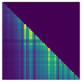
(b) Mamba

(c) Spatial-Mamba

Figure 5: Visualization of matrices ${\bm{M}}$ for linear attention, Mamba and Spatial-Mamba.

Remarks. From the above analysis, we can see that all the three paradigms — linear attention, Mamba, and Spatial-Mamba — can be modeled within a unified matrix multiplication framework, specifically $y={\bm{M}}u$. The differences lie in the structure of ${\bm{M}}$. For both linear attention and Mamba, ${\bm{M}}$ takes the form of a lower triangular matrix, whereas for Spatial-Mamba, ${\bm{M}}$ is an adjacency matrix. Fig. 5 provides a visualization of these matrices. In linear attention, the positions of brighter values remain consistent along the vertical direction, which indicates that the SA mechanism puts its focus on a small set of image tokens. Mamba, on the other hand, shows a decaying pattern over time, which is attributed to the influence of its state transition matrix $\overline{{\bm{A}}}_{t}$. This dynamic transition allows Mamba to shift its focus among previous image tokens. Unlike linear attention and Mamba, our Spatial-Mamba considers the weighted summation of all states within a broader spatial neighborhood $\Omega$, allowing for a more comprehensive representation of spatial relationships.

5 Experimental Results

In this section, we conduct a series of experiments to compare Spatial-Mamba with leading benchmark models, including those based on Convolutional Neural Networks (CNNs) (Radosavovic et al., 2020; Liu et al., 2022; Yu & Wang, 2024), Vision Transformers (Dosovitskiy et al., 2020; Liu et al., 2021; Wang et al., 2022; Hassani et al., 2023), and recent visual SSMs (Nguyen et al., 2022; Zhu et al., 2024; Liu et al., 2024; Huang et al., 2024). Following previous works (Liu et al., 2021; 2024), we train three variants of Spatial-Mamba, namely Spatial-Mamba-T, Spatial-Mamba-S and Spatial-Mamba-B. The detailed configurations are provided in Appendix A. The performance evaluation is conducted on fundamental visual tasks, including image classification, object detection, and semantic segmentation.

5.1 Image Classification on ImageNet-1K

Table 1: Comparison of classification performance on ImageNet-1K, where ‘Throughput’ is measured using an A100 GPU with an input resolution of $224\times 224$.

Arch.	Method	Im. size	#Param. (M)	FLOPs (G)	Throughput$\uparrow$	Top-1 acc.$\uparrow$
CNN	RegNetY-4G	$224^{2}$	21M	4.0G	-	80.0
	RegNetY-8G	$224^{2}$	39M	8.0G	-	81.7
	RegNetY-16G	$224^{2}$	84M	16.0G	-	82.9
	ConvNeXt-T	$224^{2}$	29M	4.5G	1189	82.1
	ConvNeXt-S	$224^{2}$	50M	8.7G	682	83.1
	ConvNeXt-B	$224^{2}$	89M	15.4G	435	83.8
Transformer	ViT-B/16	$384^{2}$	86M	55.4G	-	77.9
	ViT-L/16	$384^{2}$	307M	190.7G	-	76.5
	DeiT-S	$224^{2}$	22M	4.6G	1759	79.8
	DeiT-B	$224^{2}$	86M	17.5G	500	81.8
	DeiT-B	$384^{2}$	86M	55.4G	498	83.1
	Swin-T	$224^{2}$	28M	4.5G	1244	81.3
	Swin-S	$224^{2}$	50M	8.7G	718	83.0
	Swin-B	$224^{2}$	88M	15.4G	458	83.5
	NAT-T	$224^{2}$	28M	4.3G	-	83.2
	NAT-S	$224^{2}$	51M	7.8G	-	83.0
	NAT-B	$224^{2}$	90M	13.7G	-	84.3
SSM	S4ND-ConvNeXt-T	$224^{2}$	30M	-	683	82.2
	S4ND-ViT-B	$224^{2}$	89M	-	397	80.4
	ViM-S	$224^{2}$	26M	-	811	80.5
	VMamba-T	$224^{2}$	30M	4.9G	1686	82.6
	VMamba-S	$224^{2}$	50M	8.7G	877	83.6
	VMamba-B	$224^{2}$	89M	15.4G	646	83.9
	LocalVMamba-T	$224^{2}$	26M	5.7G	394	82.7
	LocalVMamba-S	$224^{2}$	50M	11.4G	227	83.7
	Spatial-Mamba-T	$224^{2}$	27M	4.5G	1438	83.5
	Spatial-Mamba-S	$224^{2}$	43M	7.1G	988	84.6
	Spatial-Mamba-B	$224^{2}$	96M	15.8G	665	85.3

Settings. We first evaluate the representation learning capabilities of Spatial-Mamba in image classification on ImageNet-1K (Deng et al., 2009). We adopted the experimental configurations used in previous works (Liu et al., 2021; 2024), which are detailed in Appendix A. We compare our method with state-of-the-art approaches, including RegNetY (Radosavovic et al., 2020), ConvNeXt (Liu et al., 2022), ViT (Dosovitskiy et al., 2020), DeiT (Touvron et al., 2021), Swin (Liu et al., 2021), NAT (Hassani et al., 2023), S4ND (Nguyen et al., 2022), Vim (Zhu et al., 2024), VMamba (Liu et al., 2024), and LocalVMamba (Huang et al., 2024).

Table 2: Comparison of object detection and instance segmentation performance on COCO with Mask R-CNN (He et al., 2017) detector. FLOPs are calculated with input resolution of $1280\times 800$.

Mask R-CNN 1$\times$ schedule
Backbone	AP${}^{\text{b}}\uparrow$	AP${}^{\text{b}}_{50}$$\uparrow$	AP${}^{\text{b}}_{75}$$\uparrow$	AP${}^{\text{m}}\uparrow$	AP${}^{\text{m}}_{50}$$\uparrow$	AP${}^{\text{m}}_{75}$$\uparrow$	#Param.	FLOPs
ResNet-50	38.2	58.8	41.4	34.7	55.7	37.2	44M	260G
Swin-T	42.7	65.2	46.8	39.3	62.2	42.2	48M	267G
ConvNeXt-T	44.2	66.6	48.3	40.1	63.3	42.8	48M	262G
PVTv2-B2	45.3	66.1	49.6	41.2	64.2	44.4	45M	309G
ViT-Adapter-S	44.7	65.8	48.3	39.9	62.5	42.8	48M	403G
MambaOut-T	45.1	67.3	49.6	41.0	64.1	44.1	43M	262G
VMamba-T	47.3	69.3	52.0	42.7	66.4	45.9	50M	271G
LocalVMamba-T	46.7	68.7	50.8	42.2	65.7	45.5	45M	291G
Spatial-Mamba-T	47.6	69.6	52.3	42.9	66.5	46.2	46M	261G
ResNet-101	38.2	58.8	41.4	34.7	55.7	37.2	63M	336G
Swin-S	44.8	68.6	49.4	40.9	65.3	44.2	69M	354G
ConvNeXt-S	45.4	67.9	50.0	41.8	65.2	45.1	70M	348G
PVTv2-B3	47.0	68.1	51.7	42.5	65.2	45.7	63M	397G
MambaOut-S	47.4	69.1	52.4	42.7	66.1	46.2	65M	354G
VMamba-S	48.7	70.0	53.4	43.7	67.3	47.0	70M	349G
LocalVMamba-S	48.4	69.9	52.7	43.2	66.7	46.5	69M	414G
Spatial-Mamba-S	49.2	70.8	54.2	44.0	67.9	47.5	63M	315G
Swin-B	46.9	-	-	42.3	66.3	46.0	88M	496G
ConvNeXt-B	47.0	69.4	51.7	42.7	66.3	46.0	107M	486G
PVTv2-B5	47.4	68.6	51.9	42.5	65.7	46.0	102M	557G
ViT-Adapter-B	47.0	68.2	51.4	41.8	65.1	44.9	102M	557G
MambaOut-B	47.4	69.3	52.2	43.0	66.4	46.3	100M	495G
VMamba-B	49.2	71.4	54.0	44.1	68.3	47.7	108M	485G
Spatial-Mamba-B	50.4	71.8	55.3	45.1	69.1	49.1	115M	494G
Mask R-CNN 3$\times$ MS schedule
Backbone	AP${}^{\text{b}}\uparrow$	AP${}^{\text{b}}_{50}$$\uparrow$	AP${}^{\text{b}}_{75}$$\uparrow$	AP${}^{\text{m}}\uparrow$	AP${}^{\text{m}}_{50}$$\uparrow$	AP${}^{\text{m}}_{75}$$\uparrow$	#Param.	FLOPs
Swin-T	46.0	68.1	50.3	41.6	65.1	44.9	48M	267G
ConvNeXt-T	46.2	67.9	50.8	41.7	65.0	44.9	48M	262G
NAT-T	47.7	69.0	52.6	42.6	66.1	45.9	48M	258G
VMamba-T	48.8	70.4	53.5	43.7	67.4	47.0	50M	271G
LocalVMamba-T	48.7	70.1	53.0	43.4	67.0	46.4	45M	291G
Spatial-Mamba-T	49.3	70.7	54.3	43.6	67.6	46.9	46M	261G
Swin-S	48.2	69.8	52.8	43.2	67.0	46.1	69M	354G
ConvNeXt-S	47.9	70.0	52.7	42.9	66.9	46.2	70M	348G
NAT-S	48.4	69.8	53.2	43.2	66.9	46.5	70M	330G
VMamba-S	49.9	70.9	54.7	44.2	68.2	47.7	70M	349G
LocalVMamba-S	49.9	70.5	54.4	44.1	67.8	47.4	69M	414G
Spatial-Mamba-S	50.5	71.5	55.5	44.6	68.7	47.8	63M	315G

Results. Tab. 1 presents a comprehensive comparison between Spatial-Mamba against state-of-the-art methods. Notably, Spatial-Mamba-T achieves a top-1 accuracy of 83.5%, outperforming the CNN-based ConvNext-T by 1.4% with similar amount of parameters and GFLOPs. Compared to Transformer-based methods, Spatial-Mamba-T exceeds Swin-T by 2.2% and NAT-T by 0.3%. In comparison with SSM-based methods, Spatial-Mamba-T outperforms VMamba-T by 1.0% and LocalVMamba-T by 0.8%. For other variants, Spatial-Mamba also shows advantages. Specifically, Spatial-Mamba-S and Spatial-Mamba-B achieve top-1 accuracies of 84.6% and 85.3%, respectively, surpassing NAT-S and NAT-B by margins of 1.6% and 1.0%, and VMamba-S and VMamba-B by 1.0% and 1.4%. While Spatial-Mamba-T is slightly slower than VMamba-T due to architectural differences, the Small and Base variants of Spatial-Mamba are faster than their VMamba counterparts. Moreover, both of them are significantly faster than CNN and Transformer-based methods.

5.2 Object Detection and Instance Segmentation on COCO

Settings. We evaluate Spatial-Mamba in object detection and instance segmentation tasks using COCO 2017 dataset (Lin et al., 2014) and MMDetection library (Chen et al., 2019). We adopt Mask R-CNN (He et al., 2017) as detector head, apply Spatial-Mamba-T/S/B pre-trained on ImageNet-1K as backbones. Following common practices (Liu et al., 2021; 2024), we fine-tune the pre-trained models for 12 epochs (1$\times$ schedule) and 36 epochs with multi-scale inputs (3$\times$ schedule). During training, AdamW optimizer is adopted with an initial learning rate of 0.0001 and a batch size of 16.

Results. Detailed results on COCO are reported in Tab. 2. It can be seen that all variants of Spatial-Mamba outperform their competitors under different schedules. For 1$\times$ schedule, Spatial-Mamba-T achieves a box mAP of 47.6 and a mask mAP of 42.9, surpassing Swin-T/VMamba-T by 4.9/0.3 in box mAP and 3.6/0.2 in mask mAP with fewer parameters and FLOPs, respectively. Similarly, Spatial-Mamba-S/B demonstrate superior performance to other methods under the same configuration. Furthermore, these trends of improved performance hold with the 3$\times$ multi-scale training schedule. Notably, Spatial-Mamba-S achieves the highest box mAP of 50.5 and mask mAP of 44.6, surpassing VMamba-S with a considerable gain of 0.6 and 0.4, respectively.

5.3 Semantic Segmentation on ADE20K

Table 3: Comparison of semantic segmentation on ADE20K with UPerNet (Xiao et al., 2018) segmentor. FLOPs are calculated with input resolution of $512\times 2048$. ‘SS’ and ‘MS’ represent single-scale and multi-scale testing, respectively.

Method	Crop size	mIoU (SS) $\uparrow$	mIoU (MS) $\uparrow$	#Param.	FLOPs
DeiT-S + MLN	$512^{2}$	43.1	43.8	58M	1217G
Swin-T	$512^{2}$	44.4	45.8	60M	945G
ConvNeXt-T	$512^{2}$	46.0	46.7	60M	939G
NAT-T	$512^{2}$	47.1	48.4	58M	934G
MambaOut-T	$512^{2}$	47.4	48.6	54M	938G
VMamba-T	$512^{2}$	48.0	48.8	62M	949G
LocalVMamba-T	$512^{2}$	47.9	49.1	57M	970G
Spatial-Mamba-T	$512^{2}$	48.6	49.4	57M	936G
DeiT-B + MLN	$512^{2}$	45.5	47.2	144M	2007G
Swin-S	$512^{2}$	47.6	49.5	81M	1039G
ConvNeXt-S	$512^{2}$	48.7	49.6	82M	1027G
NAT-S	$512^{2}$	48.0	49.5	82M	1010G
MambaOut-S	$512^{2}$	49.5	50.6	76M	1032G
VMamba-S	$512^{2}$	50.6	51.2	82M	1028G
LocalVMamba-S	$512^{2}$	50.0	51.0	81M	1095G
Spatial-Mamba-S	$512^{2}$	50.6	51.4	73M	992G
Swin-B	$512^{2}$	48.1	49.7	121M	1188G
ConvNeXt-B	$512^{2}$	49.1	49.9	122M	1170G
NAT-B	$512^{2}$	48.5	49.7	123M	1137G
MambaOut-B	$512^{2}$	49.6	51.0	112M	1178G
VMamba-B	$512^{2}$	51.0	51.6	122M	1170G
Spatial-Mamba-B	$512^{2}$	51.8	52.6	127M	1176G

Settings. To assess the performance of Spatial-Mamba on semantic segmentation task, we train our models with the widely used UPerNet segmentor (Xiao et al., 2018) and MMSegmenation toolkit (Contributors, 2020). Consistent with previous work (Liu et al., 2021; 2024), we pre-train our model on ImageNet-1K, and use it as the backbone to train UPerNet on ADE20K dataset (Zhou et al., 2019). This training process encompasses 160K iterations with a batch size of 16. The AdamW is used as the optimizer with a weight decay of 0.01. The learning rate is set to $6\times 10^{-5}$ with a linear learning rate decay. All the input images are cropped into $512\times 512$.

Results. The results on semantic segmentation are summarized in Tab. 3. Spatial-Mamba variants consistently achieve impressive performance. For instance, Spatial-Mamba-T attains a single-scale mIoU of 48.6 and a multi-scale mIoU of 49.4. This signifies an improvement of 1.5 mIoU over NAT-T and 0.6 mIoU over VMamba-T in single-scale input. This advantage is maintained with multi-scale input, where Spatial-Mamba-T is 1.0 mIoU higher than NAT-T and 0.6 mIoU higher than VMamba-T. Furthermore, Spatial-Mamba-B achieves the best performance with a multi-scale mIoU of 52.6.

5.4 Ablation Studies

In this section, we ablate various key components of Spatial-Mamba-T on ImageNet-1K classification task in Tab. 4. Based on the configurations of Swin-T (Liu et al., 2021), we construct the baseline model as Spatial-Mamba-T but without the SASF module. This baseline uses a $4\times 4$ convolution with a stride of $4$ as stem layer and merges $2\times 2$ neighboring patches for down-sampling.

Neighbor set. First, adjustments to the neighbor set $\Omega$ reveal that increasing the size from a $3\times 3$ neighbourhood to $5\times 5$ results in a gradual improvement in accuracy, from 82.3% to 82.5%, albeit with a corresponding decrease in throughput. Furthermore, employing a broader dilated neighbor set with factors $d=1,3,5$ increases the accuracy to 82.7%, while reducing throughput to 1158. This suggests a trade-off between speed and larger neighbor set.

Table 4: Ablation studies on Spatial-Mamba-T for neighbor set $\Omega$ and other module designs.

Module design	#Param. (M)	FLOPs (G)	Throughput $\uparrow$	Top-1 acc.$\uparrow$
Baseline	25M	4.4G	1706	82.0
$\Omega=\{3\times 3\}$	25M	4.4G	1557	82.3
$\Omega=\{5\times 5\}$	25M	4.5G	1461	82.5
$\Omega=\left\{\Omega_{d}|d=1,3,5\right\}$	25M	4.5G	1209	82.7
$+$ Overlapped Stem	27M	4.5G	1158	82.9
$+$ LPU	27M	4.5G	1065	83.3
$+$ Re-Param	27M	4.5G	1438	83.3
$+$ MESA	27M	4.5G	1438	83.5

Local enhancement. We replace the original non-overlapped stem and down-sampling layer with overlapped convolutions (refer to as ‘Overlapped Stem’ in Tab. 4), resulting in a gain of 0.2% in accuracy. We also incorporate the LPU (Guo et al., 2022), a depth-wise convolution placed at the top of each block and FFN, further increasing the accuracy by 0.4%. These modifications enrich the local information available between image patches before processing by the SASF module, enabling it to better capture structural dependencies.

Optimization. To further enhance the model efficiency, we implement the SASF module using re-parameterization techniques (Ding et al., 2022) and optimize the CUDA kernels. This accelerates the model by at least 30% and boosts the throughput from 1065 to 1438. Finally, integrating MESA (Du et al., 2022) to mitigate overfitting provides an additional 0.2% accuracy improvement.

In addition, we also provide some qualitative results in Appendix C, and a comparative analysis of the Effective Receptive Fields (ERF) (Ding et al., 2022) of various models is provided in Appendix D.

6 Conclusion

We presented in this paper Spatial-Mamba, a novel state space model designed for visual tasks. The key of Spatial-Mamba lied in the proposed structure-aware state fusion (SASF) module, which effectively captured image spatial dependencies and hence improved the contextual modeling capability. We performed extensive experiments on fundamental vision tasks of image classification, detection and segmentation. The results showed that with SASF, Spatial-Mamba surpassed the state-of-the-art state space models with only one signal scan, demonstrating its strong visual feature learning capability. We also analyzed in-depth the relationships of Spatial-Mamba with the original Mamba and linear attention, and unified them under the same matrix multiplication framework, offering a deeper understanding of the self-attention mechanism for visual representation learning.

Appendix A Detailed Experiment Settings

Network architecture. The detailed architecture of Spatial-Mamba models are outlined in Tab. 5. Following the common four-stage hierarchical framework(Liu et al., 2021; Han et al., 2024), we constructed the Spatial-Mamba models by stacking proposed Spatial-Mamba blocks at each stage. Specifically, an input image with resolution of $224\times 224$ is firstly processed by a stem layer, which consists of convolutions, Batch Normalization (BN) layers and GELU activation function. The kernel size is $3\times 3$ with a stride of 2 at first and last convolutions and a stride of 1 for the others. Each stage contains multiple Spatial-Mamba blocks, following by a down-sampling layer except the last one. The down-sampling layer consists of a $3\times 3$ convolution with a stride of 2 and a Layer Normalization (LN) layer. Each block incorporates a structure-aware SSM layer and a Feed-Forward Network (FFN), both with residual connections. The structure-aware SSM contains a SASF branch with a 2D depth-wise convolution and a multiplicative gate branch with activation function, as illustrated in Fig. 4. The expand ratio of SSM is set to 2, doubling the number of channels. We modify the embedding dimension and number of blocks to build our Spatial-Mamba-T/S/B models.

Settings for ImageNet-1K classification. The Spatial-Mamba-T/S/B models are trained from scratch for 300 epochs using AdamW optimizer with betas set to (0.9, 0.999), momentum of 0.9 and batch size of 1024. The initial learning rate is set to 0.001 with a weight decay of 0.05 and a cosine annealing learning rate schedule is adopted with a warm-up of 20 epochs. We adopt the common data augmentation strategies consisted with previous work(Liu et al., 2021; 2024). Moreover, label smoothing (0.1), exponential moving average (EMA) and MESA(Du et al., 2022) are also applied. The drop path rate is set to 0.2 for Spatial-Mamba-T, 0.3 for Spatial-Mamba-S and 0.5 for Spatial-Mamba-B.

Table 5: Architectures of Spatial-Mamba models, where Linear refers to a linear layer, DWConv represents a depth-wise convolution layer, SASF module refers to Fig. 4 in Sec. 4.2 of the main paper, and FFN is a Feed-Forward Network.

Layer	Output size	Spatial-Mamba-T	Spatial-Mamba-S	Spatial-Mamba-B
Stem	$56\times 56$	Conv $3\times 3$ stride 2, BN, GELU; Conv $3\times 3$ stride 1, BN; Conv $3\times 3$ stride 2, BN
Stage1	$28\times 28$	Spatial-Mamba Blocks	Spatial-Mamba Blocks	Spatial-Mamba Blocks
		$\left[\begin{array}[]{c}\text{Linear 64 $\rightarrow$ 128}\\ \text{DWConv 128}\\ \text{SASF 128}\\ \text{Linear 128 $\rightarrow$ 64}\\ \text{FFN 64}\end{array}\right]\times$ 2	$\left[\begin{array}[]{c}\text{Linear 64 $\rightarrow$ 128}\\ \text{DWConv 128}\\ \text{SASF 128}\\ \text{Linear 128 $\rightarrow$ 64}\\ \text{FFN 64}\end{array}\right]\times$ 2	$\left[\begin{array}[]{c}\text{Linear 96 $\rightarrow$ 192}\\ \text{DWConv 192}\\ \text{SASF 192}\\ \text{Linear 192 $\rightarrow$ 96}\\ \text{FFN 96}\end{array}\right]\times$ 2
		Down Sampling Conv $3\times 3$ stride 2, LN
Stage2	$14\times 14$	Spatial-Mamba Blocks	Spatial-Mamba Blocks	Spatial-Mamba Blocks
		$\left[\begin{array}[]{c}\text{Linear 128 $\rightarrow$ 256}\\ \text{DWConv 256}\\ \text{SASF 256}\\ \text{Linear 256 $\rightarrow$ 128}\\ \text{FFN 128}\end{array}\right]\times$ 4	$\left[\begin{array}[]{c}\text{Linear 128 $\rightarrow$ 256}\\ \text{DWConv 256}\\ \text{SASF 256}\\ \text{Linear 256 $\rightarrow$ 128}\\ \text{FFN 128}\end{array}\right]\times$ 4	$\left[\begin{array}[]{c}\text{Linear 192 $\rightarrow$ 384}\\ \text{DWConv 384}\\ \text{SASF 384}\\ \text{Linear 384 $\rightarrow$ 192}\\ \text{FFN 192}\end{array}\right]\times$ 4
		Down Sampling Conv $3\times 3$ stride 2, LN
Stage3	$7\times 7$	Spatial-Mamba Blocks	Spatial-Mamba Blocks	Spatial-Mamba Blocks
		$\left[\begin{array}[]{c}\text{Linear 256 $\rightarrow$ 512}\\ \text{DWConv 512}\\ \text{SASF 512}\\ \text{Linear 512 $\rightarrow$ 256}\\ \text{FFN 256}\end{array}\right]\times$ 8	$\left[\begin{array}[]{c}\text{Linear 256 $\rightarrow$ 512}\\ \text{DWConv 512}\\ \text{SASF 512}\\ \text{Linear 512 $\rightarrow$ 256}\\ \text{FFN 256}\end{array}\right]\times$ 21	$\left[\begin{array}[]{c}\text{Linear 384 $\rightarrow$ 768}\\ \text{DWConv 768}\\ \text{SASF 768}\\ \text{Linear 768 $\rightarrow$ 384}\\ \text{FFN 384}\end{array}\right]\times$ 21
		Down Sampling Conv $3\times 3$ stride 2, LN
Stage4	$7\times 7$	Spatial-Mamba Blocks	Spatial-Mamba Blocks	Spatial-Mamba Blocks
		$\left[\begin{array}[]{c}\text{Linear 512 $\rightarrow$ 1024}\\ \text{DWConv 1024}\\ \text{SASF 1024}\\ \text{Linear 1024 $\rightarrow$ 512}\\ \text{FFN 512}\end{array}\right]\times$ 4	$\left[\begin{array}[]{c}\text{Linear 512 $\rightarrow$ 1024}\\ \text{DWConv 1024}\\ \text{SASF 1024}\\ \text{Linear 1024 $\rightarrow$ 512}\\ \text{FFN 512}\end{array}\right]\times$ 5	$\left[\begin{array}[]{c}\text{Linear 768 $\rightarrow$ 1536}\\ \text{DWConv 1536}\\ \text{SASF 1536}\\ \text{Linear 1536 $\rightarrow$ 768}\\ \text{FFN 768}\end{array}\right]\times$ 5
Head	$1\times 1$	Average pool, Linear 1000, Softmax

Appendix B Derivation of SSM Formulas

Recall the definition of Mamba in Eq. (1), by defining the initial state $x_{0}$ as zero, the state transition equation in the recursive form can be rewritten as follows:

$$x_{t} =\overline{{\bm{A}}}_{t}x_{t-1}+\overline{{\bm{B}}}_{t}u_{t}$$ (7)

$$=\overline{{\bm{A}}}_{t}\left(\overline{{\bm{A}}}_{t-1}x_{t-2}+\overline{{\bm{B}}}_{t-1}u_{t-1}\right)+\overline{{\bm{B}}}_{t}u_{t}$$

$$=\overline{{\bm{A}}}_{t}\left(\overline{{\bm{A}}}_{t-1}\left(\overline{{\bm{A}}}_{t-2}x_{t-3}+\overline{{\bm{B}}}_{t-2}u_{t-2}\right)+\overline{{\bm{B}}}_{t-1}u_{t-1}\right)+\overline{{\bm{B}}}_{t}u_{t}$$

$$=\overline{{\bm{A}}}_{t}\overline{{\bm{A}}}_{t-1}\overline{{\bm{A}}}_{t-2}x_{t-3}+\overline{{\bm{A}}}_{t}\overline{{\bm{A}}}_{t-1}\overline{{\bm{B}}}_{t-2}u_{t-2}+\overline{{\bm{A}}}_{t}\overline{{\bm{B}}}_{t-1}u_{t-1}+\overline{{\bm{B}}}_{t}u_{t}$$

$$=\overline{{\bm{A}}}_{t}\dots\overline{{\bm{A}}}_{1}x_{0}+\overline{{\bm{A}}}_{t}\dots\overline{{\bm{A}}}_{2}\overline{{\bm{B}}}_{1}u_{1}+\cdots+\overline{{\bm{A}}}_{t}\overline{{\bm{A}}}_{t-1}\overline{{\bm{B}}}_{t-2}u_{t-2}+\overline{{\bm{A}}}_{t}\overline{{\bm{B}}}_{t-1}u_{t-1}+\overline{{\bm{B}}}_{t}u_{t}$$

$$=\sum_{s\leq t}\overline{{\bm{A}}}_{s:t}^{\times}\ \overline{{\bm{B}}}_{s}u_{s},\quad\text{where }\overline{{\bm{A}}}_{s:t}^{\times}:=\begin{cases}\overline{{\bm{A}}}_{t}\overline{{\bm{A}}}_{t-1}\dots\overline{{\bm{A}}}_{s+1}&s<t\\ 1&s=t\end{cases}.$$

By omitting term ${\bm{D}}_{t}u_{t}$ for simplicity, and multiplying by ${\bm{C}}_{t}$ according to the observation equation, we derive the final output $y_{t}=\sum_{s\leq t}{\bm{C}}_{t}\ \overline{{\bm{A}}}_{s:t}^{\times}\ \overline{{\bm{B}}}_{s}u_{s}$. Defining the input vector $u=\left[u_{1},\cdots,u_{L}\right]^{T}\in\mathbb{R}^{L}$ with sequences length $L$ and corresponding output vector $y\in\mathbb{R}^{L}$, then the above calculation can be written with in matrix multiplication framework, i.e. $y={\bm{M}}u$, where ${\bm{M}}$ is a structured lower triangular matrix and ${\bm{M}}_{ij}={\bm{C}}_{i}\overline{{\bm{A}}}_{j:i}^{\times}\overline{{\bm{B}}}_{j}$.

Similarly, we can also represent Spatial-Mamba in the same matrix transformation form. Based on Eq. (2) and Eq. (7), the SASF equation can be rewritten as $h_{t}=\sum_{k\in\Omega}\sum_{s\leq\rho_{k}(t)}\alpha_{k}\overline{{\bm{A}}}_{s:\rho_{k}(t)}^{\times}\overline{{\bm{B}}}_{s}u_{s}$. Then by multiplying ${\bm{C}}_{t}$ with out term ${\bm{D}}_{t}u_{t}$, we derive the final output of Spatial-Mamba, i.e. $y_{t}=\sum_{k\in\Omega}\sum_{s\leq\rho_{k}(t)}\alpha_{k}{\bm{C}}_{t}\overline{{\bm{A}}}_{s:\rho_{k}(t)}^{\times}\overline{{\bm{B}}}_{s}u_{s}$. This can also be concisely represented as a matrix multiplication form $y={\bm{M}}u$, where ${\bm{M}}$ is a structured adjacency matrix and ${\bm{M}}_{ij}=\sum_{k}{\bm{C}}_{i}\overline{{\bm{A}}}_{j:\rho_{k}(i)}^{\times}\overline{{\bm{B}}}_{j}$.

Appendix C Effective Receptive Field (ERF)

We compare the Effective Receptive Field (ERF) of the center pixel on popular backbone networks before and after training, as shown in Fig. 6. Our Spatial-Mamba-T and Deit-S, Vim-S and VMamba-T all show a global ERF. In addition, after training, both Vim-S and VMamba-T exhibit noticeable accumulation contributions along either horizontal or vertical directions, which is attributed to their multi-directional fusion mechanisms. In contrast, our unidirectional Spatial-Mamba-T effectively eliminates this phenomenon.

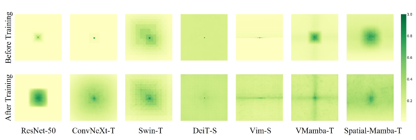
Figure 6: Comparison of Effective Receptive Field (ERF) among popular backbone networks.

Appendix D More Qualitative Results

In this section, we present the visualization results for object detection and instance segmentation tasks in Fig. 7 and for semantic segmentation task in Fig. 8. Compared with VMamba, our Spatial-Mamba demonstrates superior performance in both tasks, producing more accurate detections with higher confidence levels and more refined segmentations, particularly in areas where local structure information is crucial. For example, in the second row of Fig. 7, VMamba mistakenly identifies the shoes on a skateboard as a person, likely because observing the shoes from only four directions makes them resemble a human. Our method avoids this mistake by simultaneously perceiving the shoes and their surrounding context. Similarly, in the semantic segmentation task, as shown in the second and third rows of Fig. 8, our approach achieves more precise segmentations of the structure of trees and doors. These results highlight the effectiveness of our proposed Spatial-Mamba in leveraging local structural information for better visual understanding.

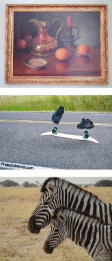
(a) Input

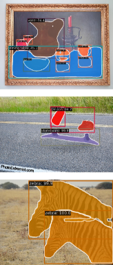
(b) VMamba

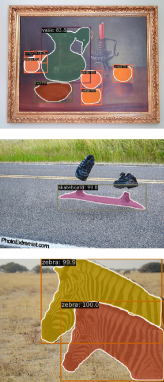
(c) Spatial-Mamba

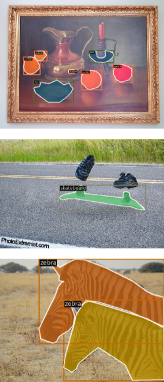
(d) Ground Truth

Figure 7: Visualization examples for object detection and instance segmentation tasks on COCO dataset with Mask R-CNN 1$\times$ schedule between VMamba and Spatial-Mamba.

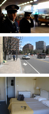
(a) Input

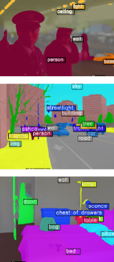
(b) VMamba

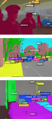
(c) Spatial-Mamba

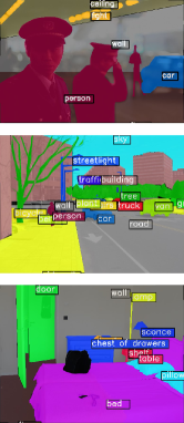
(d) Ground Truth

Figure 8: Visualization examples for semantic segmentation task on ADE20K dataset with single-scale inputs between VMamba and Spatial-Mamba.

References

- Baron et al. (2023) Ethan Baron, Itamar Zimerman, and Lior Wolf. A 2-dimensional state space layer for spatial inductive bias. In The Twelfth International Conference on Learning Representations, 2023.
- Chen et al. (2024) Guo Chen, Yifei Huang, Jilan Xu, Baoqi Pei, Zhe Chen, Zhiqi Li, Jiahao Wang, Kunchang Li, Tong Lu, and Limin Wang. Video mamba suite: State space model as a versatile alternative for video understanding. arXiv preprint arXiv:2403.09626, 2024.
- Chen et al. (2019) Kai Chen, Jiaqi Wang, Jiangmiao Pang, Yuhang Cao, Yu Xiong, Xiaoxiao Li, Shuyang Sun, Wansen Feng, Ziwei Liu, Jiarui Xu, et al. Mmdetection: Open mmlab detection toolbox and benchmark. arXiv preprint arXiv:1906.07155, 2019.
- Contributors (2020) MMSegmentation Contributors. Mmsegmentation: Openmmlab semantic segmentation toolbox and benchmark, 2020.
- Dao & Gu (2024) Tri Dao and Albert Gu. Transformers are ssms: Generalized models and efficient algorithms through structured state space duality. arXiv preprint arXiv:2405.21060, 2024.
- Deng et al. (2009) Jia Deng, Wei Dong, Richard Socher, Li-Jia Li, Kai Li, and Li Fei-Fei. Imagenet: A large-scale hierarchical image database. In 2009 IEEE conference on computer vision and pattern recognition, pp. 248–255. Ieee, 2009.
- Ding et al. (2022) Xiaohan Ding, Xiangyu Zhang, Jungong Han, and Guiguang Ding. Scaling up your kernels to 31x31: Revisiting large kernel design in cnns. In Proceedings of the IEEE/CVF conference on computer vision and pattern recognition, pp. 11963–11975, 2022.
- Dosovitskiy et al. (2020) Alexey Dosovitskiy, Lucas Beyer, Alexander Kolesnikov, Dirk Weissenborn, Xiaohua Zhai, Thomas Unterthiner, Mostafa Dehghani, Matthias Minderer, Georg Heigold, Sylvain Gelly, et al. An image is worth 16x16 words: Transformers for image recognition at scale. arXiv preprint arXiv:2010.11929, 2020.
- Du et al. (2022) Jiawei Du, Daquan Zhou, Jiashi Feng, Vincent Tan, and Joey Tianyi Zhou. Sharpness-aware training for free. Advances in Neural Information Processing Systems, 35:23439–23451, 2022.
- Friston et al. (2003) Karl J Friston, Lee Harrison, and Will Penny. Dynamic causal modelling. Neuroimage, 19(4):1273–1302, 2003.
- Fu et al. (2022) Daniel Y Fu, Tri Dao, Khaled K Saab, Armin W Thomas, Atri Rudra, and Christopher Ré. Hungry hungry hippos: Towards language modeling with state space models. arXiv preprint arXiv:2212.14052, 2022.
- Gu & Dao (2023) Albert Gu and Tri Dao. Mamba: Linear-time sequence modeling with selective state spaces. arXiv preprint arXiv:2312.00752, 2023.
- Gu et al. (2020) Albert Gu, Tri Dao, Stefano Ermon, Atri Rudra, and Christopher Ré. Hippo: Recurrent memory with optimal polynomial projections. Advances in neural information processing systems, 33:1474–1487, 2020.
- Gu et al. (2021a) Albert Gu, Karan Goel, and Christopher Ré. Efficiently modeling long sequences with structured state spaces. arXiv preprint arXiv:2111.00396, 2021a.
- Gu et al. (2021b) Albert Gu, Isys Johnson, Karan Goel, Khaled Saab, Tri Dao, Atri Rudra, and Christopher Ré. Combining recurrent, convolutional, and continuous-time models with linear state space layers. Advances in neural information processing systems, 34:572–585, 2021b.
- Guo et al. (2024) Hang Guo, Jinmin Li, Tao Dai, Zhihao Ouyang, Xudong Ren, and Shu-Tao Xia. Mambair: A simple baseline for image restoration with state-space model. arXiv preprint arXiv:2402.15648, 2024.
- Guo et al. (2022) Jianyuan Guo, Kai Han, Han Wu, Yehui Tang, Xinghao Chen, Yunhe Wang, and Chang Xu. Cmt: Convolutional neural networks meet vision transformers. In Proceedings of the IEEE/CVF conference on computer vision and pattern recognition, pp. 12175–12185, 2022.
- Gupta et al. (2022) Ankit Gupta, Albert Gu, and Jonathan Berant. Diagonal state spaces are as effective as structured state spaces. Advances in Neural Information Processing Systems, 35:22982–22994, 2022.
- Hafner et al. (2019) Danijar Hafner, Timothy Lillicrap, Jimmy Ba, and Mohammad Norouzi. Dream to control: Learning behaviors by latent imagination. arXiv preprint arXiv:1912.01603, 2019.
- Han et al. (2024) Dongchen Han, Ziyi Wang, Zhuofan Xia, Yizeng Han, Yifan Pu, Chunjiang Ge, Jun Song, Shiji Song, Bo Zheng, and Gao Huang. Demystify mamba in vision: A linear attention perspective. arXiv preprint arXiv:2405.16605, 2024.
- Hassani et al. (2023) Ali Hassani, Steven Walton, Jiachen Li, Shen Li, and Humphrey Shi. Neighborhood attention transformer. In Proceedings of the IEEE/CVF Conference on Computer Vision and Pattern Recognition, pp. 6185–6194, 2023.
- He et al. (2024a) Haoyang He, Yuhu Bai, Jiangning Zhang, Qingdong He, Hongxu Chen, Zhenye Gan, Chengjie Wang, Xiangtai Li, Guanzhong Tian, and Lei Xie. Mambaad: Exploring state space models for multi-class unsupervised anomaly detection. arXiv preprint arXiv:2404.06564, 2024a.
- He et al. (2017) Kaiming He, Georgia Gkioxari, Piotr Dollár, and Ross Girshick. Mask r-cnn. In Proceedings of the IEEE international conference on computer vision, pp. 2961–2969, 2017.
- He et al. (2024b) Wei He, Kai Han, Yehui Tang, Chengcheng Wang, Yujie Yang, Tianyu Guo, and Yunhe Wang. Densemamba: State space models with dense hidden connection for efficient large language models. arXiv preprint arXiv:2403.00818, 2024b.
- Hu et al. (2024) Vincent Tao Hu, Stefan Andreas Baumann, Ming Gui, Olga Grebenkova, Pingchuan Ma, Johannes Fischer, and Bjorn Ommer. Zigma: Zigzag mamba diffusion model. arXiv preprint arXiv:2403.13802, 2024.
- Huang et al. (2024) Tao Huang, Xiaohuan Pei, Shan You, Fei Wang, Chen Qian, and Chang Xu. Localmamba: Visual state space model with windowed selective scan. arXiv preprint arXiv:2403.09338, 2024.
- Kalman (1960) Rudolph Emil Kalman. A new approach to linear filtering and prediction problems. 1960.
- Katharopoulos et al. (2020) Angelos Katharopoulos, Apoorv Vyas, Nikolaos Pappas, and François Fleuret. Transformers are rnns: Fast autoregressive transformers with linear attention. In International conference on machine learning, pp. 5156–5165. PMLR, 2020.
- Li et al. (2024) Kunchang Li, Xinhao Li, Yi Wang, Yinan He, Yali Wang, Limin Wang, and Yu Qiao. Videomamba: State space model for efficient video understanding. arXiv preprint arXiv:2403.06977, 2024.
- Liao et al. (2024) Weibin Liao, Yinghao Zhu, Xinyuan Wang, Cehngwei Pan, Yasha Wang, and Liantao Ma. Lightm-unet: Mamba assists in lightweight unet for medical image segmentation. arXiv preprint arXiv:2403.05246, 2024.
- Lin et al. (2014) Tsung-Yi Lin, Michael Maire, Serge Belongie, James Hays, Pietro Perona, Deva Ramanan, Piotr Dollár, and C Lawrence Zitnick. Microsoft coco: Common objects in context. In Computer Vision–ECCV 2014: 13th European Conference, Zurich, Switzerland, September 6-12, 2014, Proceedings, Part V 13, pp. 740–755. Springer, 2014.
- Liu et al. (2024) Yue Liu, Yunjie Tian, Yuzhong Zhao, Hongtian Yu, Lingxi Xie, Yaowei Wang, Qixiang Ye, and Yunfan Liu. Vmamba: Visual state space model. arXiv preprint arXiv:2401.10166, 2024.
- Liu et al. (2021) Ze Liu, Yutong Lin, Yue Cao, Han Hu, Yixuan Wei, Zheng Zhang, Stephen Lin, and Baining Guo. Swin transformer: Hierarchical vision transformer using shifted windows. In Proceedings of the IEEE/CVF international conference on computer vision, pp. 10012–10022, 2021.
- Liu et al. (2022) Zhuang Liu, Hanzi Mao, Chao-Yuan Wu, Christoph Feichtenhofer, Trevor Darrell, and Saining Xie. A convnet for the 2020s. In Proceedings of the IEEE/CVF conference on computer vision and pattern recognition, pp. 11976–11986, 2022.
- Ma et al. (2024) Jun Ma, Feifei Li, and Bo Wang. U-mamba: Enhancing long-range dependency for biomedical image segmentation. arXiv preprint arXiv:2401.04722, 2024.
- Mo & Tian (2024) Shentong Mo and Yapeng Tian. Scaling diffusion mamba with bidirectional ssms for efficient image and video generation. arXiv preprint arXiv:2405.15881, 2024.
- Nguyen et al. (2022) Eric Nguyen, Karan Goel, Albert Gu, Gordon Downs, Preey Shah, Tri Dao, Stephen Baccus, and Christopher Ré. S4nd: Modeling images and videos as multidimensional signals with state spaces. Advances in neural information processing systems, 35:2846–2861, 2022.
- Qiao et al. (2024) Yanyuan Qiao, Zheng Yu, Longteng Guo, Sihan Chen, Zijia Zhao, Mingzhen Sun, Qi Wu, and Jing Liu. Vl-mamba: Exploring state space models for multimodal learning. arXiv preprint arXiv:2403.13600, 2024.
- Radosavovic et al. (2020) Ilija Radosavovic, Raj Prateek Kosaraju, Ross Girshick, Kaiming He, and Piotr Dollár. Designing network design spaces. In Proceedings of the IEEE/CVF conference on computer vision and pattern recognition, pp. 10428–10436, 2020.
- Shi et al. (2024) Yuan Shi, Bin Xia, Xiaoyu Jin, Xing Wang, Tianyu Zhao, Xin Xia, Xuefeng Xiao, and Wenming Yang. Vmambair: Visual state space model for image restoration. arXiv preprint arXiv:2403.11423, 2024.
- Smith et al. (2022) Jimmy TH Smith, Andrew Warrington, and Scott W Linderman. Simplified state space layers for sequence modeling. arXiv preprint arXiv:2208.04933, 2022.
- Touvron et al. (2021) Hugo Touvron, Matthieu Cord, Matthijs Douze, Francisco Massa, Alexandre Sablayrolles, and Hervé Jégou. Training data-efficient image transformers & distillation through attention. In International conference on machine learning, pp. 10347–10357. PMLR, 2021.
- Wang et al. (2022) Wenhai Wang, Enze Xie, Xiang Li, Deng-Ping Fan, Kaitao Song, Ding Liang, Tong Lu, Ping Luo, and Ling Shao. Pvt v2: Improved baselines with pyramid vision transformer. Computational Visual Media, 8(3):415–424, 2022.
- Williams & Lawrence (2007) Robert L. Williams and Douglas A. Lawrence. Linear state-space control systems —— observability. 10.1002/9780470117873:149–184, 2007.
- Xiao et al. (2018) Tete Xiao, Yingcheng Liu, Bolei Zhou, Yuning Jiang, and Jian Sun. Unified perceptual parsing for scene understanding. In Proceedings of the European conference on computer vision (ECCV), pp. 418–434, 2018.
- Xiao et al. (2024) Yicheng Xiao, Lin Song, Shaoli Huang, Jiangshan Wang, Siyu Song, Yixiao Ge, Xiu Li, and Ying Shan. Grootvl: Tree topology is all you need in state space model. arXiv preprint arXiv:2406.02395, 2024.
- Yang et al. (2024) Chenhongyi Yang, Zehui Chen, Miguel Espinosa, Linus Ericsson, Zhenyu Wang, Jiaming Liu, and Elliot J Crowley. Plainmamba: Improving non-hierarchical mamba in visual recognition. arXiv preprint arXiv:2403.17695, 2024.
- Yao et al. (2024) Jing Yao, Danfeng Hong, Chenyu Li, and Jocelyn Chanussot. Spectralmamba: Efficient mamba for hyperspectral image classification. arXiv preprint arXiv:2404.08489, 2024.
- Yu (2015) F Yu. Multi-scale context aggregation by dilated convolutions. arXiv preprint arXiv:1511.07122, 2015.
- Yu & Wang (2024) Weihao Yu and Xinchao Wang. Mambaout: Do we really need mamba for vision? arXiv preprint arXiv:2405.07992, 2024.
- Yue & Li (2024) Yubiao Yue and Zhenzhang Li. Medmamba: Vision mamba for medical image classification. arXiv preprint arXiv:2403.03849, 2024.
- Zhou et al. (2019) Bolei Zhou, Hang Zhao, Xavier Puig, Tete Xiao, Sanja Fidler, Adela Barriuso, and Antonio Torralba. Semantic understanding of scenes through the ade20k dataset. International Journal of Computer Vision, 127:302–321, 2019.
- Zhu et al. (2024) Lianghui Zhu, Bencheng Liao, Qian Zhang, Xinlong Wang, Wenyu Liu, and Xinggang Wang. Vision mamba: Efficient visual representation learning with bidirectional state space model. arXiv preprint arXiv:2401.09417, 2024.