Identification by non-Gaussianity in structural threshold and smooth transition vector autoregressive models

Savi Virolainen
University of Helsinki

Linear structural vector autoregressive models can be identified statistically without imposing restrictions on the model if the shocks are mutually independent and at most one of them is Gaussian. We show that this result extends to structural threshold and smooth transition vector autoregressive models incorporating a time-varying impact matrix defined as a weighted sum of the impact matrices of the regimes. Our empirical application studies the effects of the climate policy uncertainty shock on the U.S. macroeconomy. In a structural logistic smooth transition vector autoregressive model consisting of two regimes, we find that a positive climate policy uncertainty shock decreases production in times of low economic policy uncertainty but slightly increases it in times of high economic policy uncertainty. The introduced methods are implemented to the accompanying R package sstvars.

Keywords: smooth transition vector autoregression, nonlinear SVAR, identification by non-Gaussianity, non-Gaussian SVAR

1 Introduction

Smooth transition vector autoregressive (STVAR) models (Anderson and Vahid, 1998) have been widely adopted in empirical macroeconomics due to their ability to flexibly capture nonlinear data generating dynamics and gradual shifts in parameter values. Such variation may arise due to wars, business cycle fluctuations, or policy shifts, for example. Structural STVAR model are particularly useful, as they facilitate tracing out the causal effects of economic shocks, which may vary in time depending on the initial state of the economy as well as on the sign and size of the shock. In order to estimate their effects, the economic shocks need to be identified. Conventional identification methods typically rely on restrictive assumptions such as zero contemporaneous interactions among some of the variables or long-term neutrality of the shocks. Such restrictions are advantageous when based on economic reasoning, but often they are economically implausible and imposed just to obtain some identification reasonable enough. To overcome this issue, statistical identification methods have been developed.

There are two main branches in the statistical identification literature: identification by heteroskedasticity (Rigobon, 2003, Lanne et al., 2010, Bacchiocchi and Fanelli, 2015, Lütkepohl and Netšunajev, 2017, Virolainen, forthcoming, and others) and identification by non-Gaussianity (Lanne et al., 2017, Maxand, 2020, Lanne and Luoto, 2021, Lanne et al., 2023, Anttonen et al., forthcoming, and others). Under certain statistical conditions, both types of identification methods typically identify the shocks of a linear structural vector autoregressive (SVAR) model without imposing further restrictions. However, identification by heteroskedasticity has the major drawback in nonlinear SVAR models that for each shock, it restricts the relative magnitudes of the impact responses of the variables to stay constant over time (see the discussion in Virolainen, forthcoming, Sections 3.1 and 4). This is an undesired property, as it would be generally desirable to accommodate time-variation in the (relative) impact responses. Bacchiocchi and Fanelli (2015) propose an alternative framework for identification by heteroskedasticity, and allow for variation in the impact effects of the shocks across the volatility regimes, but their method requires imposing a number of unstable zero impact effect restrictions that can be challenging to justify economically. To the best our knowledge, identifying nonlinear SVAR models by non-Gaussianity has not been studied in the previous literature.

This paper contributes to the literature on identification by non-Gaussianity by extending the framework proposed by Lanne et al. (2017) to STVAR models (we consider threshold vector autoregressive models, Tsay, 1998, as special cases of STVAR models). A key difference to linear vector autoregressive (VAR) models is that in STVAR models, the impact matrix should generally be time-varying to facilitate time-variation in the impact responses of the variables to the shocks. This complicates the identification, since instead of identifying a static impact matrix as in Lanne et al. (2017), the parameters of the time-varying impact matrix need to be identified. Similarly to Lanne et al. (2017), however, it turns out that a sufficient identification condition is that the shocks are mutually independent and at most one of them is Gaussian. We show that under this condition, when the impact matrix of a STVAR model is defined as a weighted sum of the impact matrices of the regimes, the shocks are readily identified. The weights of the impact matrices are the transition weights of the regimes, which we assume to be either exogenous or, for a $p$th order model, functions of the preceding $p$ observations.

In line with statistical identification literature, labelling the identified shocks by the economic shocks of interest requires external information, for instance, in the form of economic short-run restrictions. Due to identification, such overidentifying restrictions are testable. In turns out that the identification is often weak with respect to the ordering and signs of the columns of the impact matrices of the some of the regimes. It is, however, important that the columns of the impact matrices are in a correct order, because a shock is labelled to one of the columns of the time-varying impact matrix, and it thus needs to be labelled to the same column in each of the impact matrices of the regimes. Using an inappropriate ordering or signs of the columns in some of the regime-specific impact matrices would, hence, result in impulse response functions that do not estimate the effects of the intended shock but of a linear combination of the structural shocks. Therefore, we propose a procedure to facilitate reliable labelling of the shocks by making use of short-run sign restrictions, which can be also be combined with testable zero restrictions and other types of information. In addition to introducing the identification results, we make use of the results of Saikkonen (2008) to present sufficient conditions for establishing stationarity, ergodicity, and mixing properties of our structural STVAR model. Our identification results do not, however, require stationarity.

Developments related to ours include the new framework of Morioka et al. (2021) called independent innovation analysis (IIA). Morioka et al. (2021) propose using IIA for directly estimating the (conditionally) contemporaneously independent innovations of a general nonlinear VAR model without assuming a specific functional form for the model. They show that under a certain set of (fairly general) assumptions, their method consistently estimates the independent innovations up to permutation and scalar component-wise invertible transformations. In applied macroeconometrics, the main interest is, however, typically in computing the (generalized) impulse response functions or performing other analyses that require obtaining an estimate for the parameters of the model. Estimating the parameters of a STVAR model using the framework of Morioka et al. (2021) requires first estimating the independent innovations using a specific machine learning algorithm (see Morioka et al., 2021), and then using the estimates of the innovations to obtain estimates of the parameters. However, it is not obvious how to estimate the parameters of the model from the innovations obtained by IIA, as they are identified only up to permutation and component-wise invertible transformations, and different parameter estimates would be obtained with different transformations. Moreover, Morioka et al. (2021) assume that the innovations are from a distribution in an exponential family, thereby excluding various distributions such as the popular Student’s $t$ distribution. Our approach, in turn, facilitates estimating the parameters directly by the method of maximum likelihood, and it does not exclude distributions of the independent shocks other than Gaussian distribution and those with infinite variance.

Our empirical application studies the macroeconomic effects of climate policy uncertainty shocks and consider a monthly U.S. data from 1987:4 to 2024:2. Following Gavriilidis et al. (2023), we measure climate policy uncertainty (CPU) with the CPU index (Gavriilidis, 2021), which is constructed based on the amount of newspaper coverage on topics related climate policy uncertainty. We fit a two-regime logistic STVAR model (Anderson and Vahid, 1998) using the first lag of the economic policy uncertainty index (Baker et al., 2016) as the switching variable and allowing for smooth transitions in the intercept parameters as well as in the impact matrix. We find that a positive CPU shock decreases production in times of low economic policy uncertainty, while production slightly increases in times of high economic policy uncertainty. Consumer prices, in turn, increase more significantly when the level of economic policy uncertainty is high than when it is low. Our results are, therefore, somewhat contrary to Gavriilidis et al. (2023), who found a positive CPU decreasing real activity and increasing prices, thus, transmitting to the U.S. economy as a supply shock.

The rest of this paper is organized as follows. Section 2 presents the considered framework of reduced form STVAR models and provides examples of the covered models. Section 3 discusses identification of the shocks in structural STVAR model, presents our results on identification by non-Gaussianity, and describes a procedure to facilitate reliable labelling the shocks in the presence of weak identification. Section 4 presents sufficient conditions for establishing stationarity, ergodicity, and mixing properties of our structural STVAR model. Section 5 discusses estimation of the parameters by the method of maximum likelihood, Section 6 presents the empirical application, and Section 7 concludes. Appendices give proofs for the stated lemmas, propositions, and theorem, as well as details related to the empirical application. Finally, the introduced methods have been implemented to the accompanying R package sstvars (Virolainen, 2024).

2 Reduced form STVAR models

Let $y_{t}$, $t=1,2,...$, be the $d$-dimensional time series of interest and $\mathcal{F}_{t-1}$ denote the $\sigma$-algebra generated by the random vectors $\{y_{t-j},j>0\}$. We consider STVAR models with $M$ regimes and autoregressive order $p$ assumed to satisfy

$$y_{t} =\sum_{m=1}^{M}\alpha_{m,t}\mu_{m,t}+u_{t},\quad u_{t}\sim MD(0,\Omega_{y,t},\nu),$$ (2.1)

$$\mu_{m,t} =\phi_{m,0}+\sum_{i=1}^{p}A_{m,i}y_{t-i},\quad m=1,...,M,$$ (2.2)

where $\phi_{1,0},...,\phi_{M,0}\in\mathbb{R}^{d}$, $m=1,...,M$, are the intercept parameters; $A_{1,i},...,A_{M,i}\in\mathbb{R}^{d\times d}$, $i=1,...,p$, are the autoregression matrices; $u_{t}$ is a martingale difference sequence of reduced form innovations; $\Omega_{y,t}$ is the positive definite conditional covariance matrix of $u_{t}$ (conditional on $\mathcal{F}_{t-1}$), which may depend on $\alpha_{1,t},...,\alpha_{M,t}$ and $y_{t-1},...,y_{t-p}$; and $\nu$ collects any other parameters the distribution of $u_{t}$ depends on. The transition weights $\alpha_{m,t}$ are assumed to be either nonrandom and exogenous or $\mathcal{F}_{t-1}$-measurable functions of $\{y_{t-j},j=1,...,p\}$, and they satisfy $\sum_{m=1}^{M}\alpha_{m,t}=1$ at all $t$. Thus, the types of transition weights typically used in macroeconomic applications are accommodated. The transition weights express the proportions of the regimes the process is on at each point of time and determine how the process shifts between them.

It is easy to see that, conditional on $\mathcal{F}_{t-1}$, the conditional mean of the above-described process is $\mu_{y,t}\equiv E[y_{t}|\mathcal{F}_{t-1}]=\sum_{m=1}^{M}\alpha_{m,t}\mu_{m,t}$, a a weighted sum the regime-specific means $\mu_{m,t}$ with the weights given by the transition weights $\alpha_{m,t}$. The conditional covariance matrix is $\Omega_{y,t}$, but discussion on its specification is postponed to Section 3. See Hubrich and Teräsvirta (2013) for survey on STVAR literature, including also specifications more general than ours.

It is often assumed that the coefficient matrices $A_{m,i}$, $i=1,...,p$, satisfy the usual stability condition $\det\left(I_{d}-\sum_{i=1}^{p}A_{m,i}z^{i}\right)\neq 0\ \ \text{for}\ \ |z|\leq 1,$ for each of the regimes $m=1,...,M$. However, this condition does not necessarily ensure that the model is stationary (see Kheifets and Saikkonen, 2020, and the references therein). If the transition weights are exogenous, it might be particularly challenging to establish the stationarity of the model. Assuming endogenous transition weights, we present sufficient conditions for establishing ergodicity, stationary, and mixing properties of our structural STVAR model in Section 4. Nevertheless, our main identification results discussed in Section 3 do not require stationarity of the model.

The above-described framework of STVAR models accommodates various types of transition weights employed in empirical macroeconomics. To provide a few examples, consider first the Threshold VAR (TVAR) models (Tsay, 1998), which are obtained from (2.1) and (2.2) by assuming that the transition weights are defined as

$$\alpha_{m,t}=\left\{\begin{matrix}1&\text{if}\ \ r_{m-1}<z_{t}\leq r_{m},\\ 0&\text{otherwise},\phantom{aaaaaaa}\end{matrix}\right.$$ (2.3)

where $r_{0}\equiv-\infty$, $r_{M}\equiv\infty$, $m=1,...,M$, are threshold parameters, and $z_{t}$ is a switching variable. At each $t$‚ the model defined in Equations (2.1), (2.2) and (2.3) reduces to a linear VAR corresponding to one of the regimes that is determined according to the level of the switching variable $z_{t}$, which can be either exogenous or a lagged endogenous variable.

Another popular specification is to assume two-regimes ($M=2$) and logistic transition weights. In the logistic STVAR model (Anderson and Vahid, 1998), the transition weights vary according a logistic function as

$$\alpha_{1,t}=1-\alpha_{2,t}\ \ \text{and}\ \ \alpha_{2,t}=[1+\exp\{-\gamma(z_{t}-c)\}]^{-1},$$ (2.4)

where $z_{t}$ is the switching variable, $c\in\mathbb{R}$ is a location parameter, and $\gamma>0$ is a scale parameter. The location parameter $c$ determines the mid point of the transition function, i.e., the value of the (lagged) switching variable when the weights are equal. The scale parameter $\gamma$, in turn, determines the smoothness of the transitions (smaller $\gamma$ implies smoother transitions), and it is assumed strictly positive so that $\alpha_{2,t}$ is increasing in $z_{t}$. The switching variable $z_{t}$ can be an exogenous variable, a lagged endogenous variable, or it can be a linear combination of multiple such variables.

In addition specifying the transition weights or error processes $u_{t}$ in various ways, different types of models can be obtained by imposing parameter restrictions to the model defined in (2.1)-(2.2). For instance, a model that is linear the in the autoregressive (AR) coefficients is obtained by assuming that they are constants across the regimes, i.e., $A_{m,i}=A_{i}$ and $\phi_{m,0}=\phi_{0}$ for all $i=1,...,p$ and $M=1,...,M$. The resulting model then simplifies to

$$y_{t}=\phi_{0}+\sum_{i=1}^{p}A_{i}y_{t-i}+u_{t},\quad u_{t}\sim MD(0,\Omega_{y,t},\nu).$$ (2.5)

The linear model in (2.5) is typically substantially easier to estimate and has much less parameters than the fully nonlinear specification in (2.1)-(2.2), so it is more feasible in large scale VAR analyses, but it can still accommodate shifts in the volatility regime through the error process $u_{t}$.

Imposing constant AR matrices across the regimes but allowing the intercepts to vary in time is a particularly useful special case of (2.1)-(2.2), as constant AR matrices substantially decreases the number parameters compared to the fully nonlinear specification, but it sill allows time-varying condition mean via the time-varying intercepts as well as shifts in the volatility regime through the error process $u_{t}$. This specification is obtained from (2.1)-(2.2) by assuming $A_{m,i}=A_{i}$ for all $i=1,...,p$ and $M=1,...,M$, simplifying the model to:

$$y_{t}=\sum_{m=1}^{M}\alpha_{m,t}\phi_{m,0}+\sum_{i=1}^{p}A_{i}y_{t-i}+u_{t},\quad u_{t}\sim MD(0,\Omega_{y,t},\nu).$$ (2.6)

Finally, note that while we focus on TVAR and STVAR models here for concreteness and because these models are implemented to the accompanying R package sstvars (Virolainen, 2024), the identification results of this paper directly extend to other nonlinear SVAR models. This includes also models incorporating discrete regime switches such as Markov-Switching VAR models (Krolzig, 1997) and mixture VAR models (e.g., Fong et al., 2007), and more generally models whose impact matrix is defined as a weighted sum of the impact matrices of the regimes and the time $t$ weights are known at the time $t$.

3 Structural STVAR models identified by non-Gaussianity

3.1 Structural STVAR models

A structural STVAR model is obtained from the reduced form model defined in Section 2 by identifying the serially and mutually uncorrelated structural shocks $e_{t}=(e_{1t},...,e_{dt})$ $(d\times 1)$ from the reduced form innovations $u_{t}$. Specifically, the structural shocks are recovered from the reduced form shocks with the transformation

$$e_{t}=B_{y,t}^{-1}u_{t},$$ (3.1)

where $B_{y,t}$ is an invertible ($d\times d$) impact matrix that governs the contemporaneous relationships of the shocks and may depend on $\alpha_{1,t},...,\alpha_{M,t}$ and $y_{t-1},...,y_{t-p}$. In other words, assuming a unit variance normalization for the structural shocks, the identification problem amounts to finding an impact matrix $B_{y,t}$ such that $\Omega_{y,t}=B_{y,t}B_{y,t}^{\prime}$. The impact matrix is not, however, generally uniquely identified without imposing further restrictions on the model, since there exists many such decompositions of $\Omega_{y,t}$. Various types of restrictions that recover the structural shocks have been proposed in the literature. Many of them are discussed in Ramey (2016) and Kilian and Lütkepohl (2017), for example.

Following the literature on statistical identification by non-Gaussianity in the framework proposed by Lanne et al. (2017), our identifying restriction is that the shocks are mutually independent and that at most one of them is Gaussian. In the case of Gaussian shocks, different decompositions of the conditional covariance matrix $\Omega_{y,t}=B_{y,t}B_{y,t}^{\prime}$ lead to observationally equivalent models. But when the shocks are mutually independent and at most of them is Gaussian, different decompositions generally lead to models that are not observationally equivalent (see Lanne et al., 2017). This implies that if a model with mutually independent non-Gaussian shocks is parametrized with the conditional covariance matrix $\Omega_{y,t}$, the decomposition that identifies the shocks needs to be imposed prior to estimation. In this case, the identification problem does not deviate from the conventional Gaussian specification. Therefore, instead of parametrizing the model with the conditional covariance matrix, we parametrize the structural model directly with the impact matrix $B_{y,t}$ and study its identification. Lanne et al. (2017) show that in a linear SVAR model incorporating mutually independent shocks at most one of which is Gaussian, the impact matrix is readily identified (up ordering and scales of its columns) without additional restrictions. We extend their result to a time-varying impact matrix.

In order to parametrize the model directly with the impact matrix, we make the identity $u_{t}=B_{y,t}e_{t}$ explicit in Equation (2.1) as

$$y_{t}=\sum_{m=1}^{M}\alpha_{m,t}\left(\phi_{m,0}+\sum_{i=1}^{p}A_{m,i}y_{t-i}\right)+B_{y,t}e_{t},\quad e_{t}\sim IID(0,I_{d},\nu),$$ (3.2)

where $e_{t}$ are independent and identically distributed structural errors with identity covariance matrix and a distribution that may depend on the parameter $\nu$.

Since we incorporate time-variation in the impact matrix, its functional form needs to be specified. A natural specification for a STVAR model is to assume a constant impact matrix for each of the regimes and define the impact matrix of the process to be their weighted sum as

$$B_{y,t}=\sum_{m=1}^{M}\alpha_{m,t}B_{m},$$ (3.3)

where $B_{1},...,B_{M}$ are invertible $(d\times d)$ impact matrices of the regimes. Also the impact matrix $B_{y,t}$ needs to be invertible to ensure positive definiteness of the conditional covariance matrix, which does not automatically follow from the invertibility of $B_{1},...,B_{M}$. Nevertheless, it turns out that $B_{y,t}$ defined in (3.3) is invertible for all $t$ almost everywhere in $[B_{1}:...:B_{M}]\in\mathbb{R}^{d\times dM}$, as is stated in the following lemma (which is proven in Appendix A.1).

Lemma 1.

Suppose $B_{1},...,B_{M}$ are invertible $(d\times d)$ matrices and $\alpha_{1,t},...,\alpha_{M,t}$ scalars such that $\sum_{m=1}^{M}\alpha_{m,t}=1$ and $\alpha_{m,t}\geq 0$ for all $t$ and $m=1,...,M$. Then, the matrix $B_{y,t}=\sum_{m=1}^{M}\alpha_{m,t}B_{m}$ is invertible for all $t$ almost everywhere in $[B_{1}:...:B_{M}]\in\mathbb{R}^{d\times dM}$.

The result of Lemma 1 holds almost everywhere in $[B_{1}:...:B_{M}]\in\mathbb{R}^{d\times dM}$, which means that the set where the matrices $B_{1},...,B_{M}$ that are such that $B_{y,t}$ is singular for some $t$ has a Lebesgue measure zero. This implies that invertible matrices $B_{1},...,B_{M}$ generally lead to an invertible impact matrix $B_{y,t}$, excluding some specific values of $B_{1},...,B_{M}$ for which this result does not hold (e.g., if $B_{2}=-B_{1}$, $B_{y,t}=0$ when $\alpha_{1,t}=\alpha_{2,t}=0.5$). To further improve intuition, observe that the result of Lemma 1 implies that if the matrices $B_{1},...,B_{M}$ are drawn by random from a continuous distribution, the probability of obtaining matrices such that $B_{y,t}$ is singular for some $t$ is zero. In practice, the parameter space should be simply restricted in the estimation so that parameter values leading to an impact matrix $B_{t}$ that is singular for some $t=1,...,T$ are excluded.

Assuming impact matrix of the form (3.3), the conditional covariance matrix of $y_{t}$, conditional on $\mathcal{F}_{t-1}$, is obtained as

$$\Omega_{y,t}=\left(\sum_{m=1}^{M}\alpha_{m,t}B_{m}\right)\left(\sum_{m=1}^{M}\alpha_{m,t}B_{m}\right)^{\prime}=\sum_{m=1}^{M}\alpha_{m,t}^{2}\Omega_{m}+\sum_{m=1}^{M}\sum_{n=1,n\neq m}^{M}\alpha_{m,t}\alpha_{n,t}\Omega_{m,n},$$ (3.4)

where $\Omega_{m}\equiv B_{m}B_{m}^{\prime}$ and $\Omega_{m,n}\equiv B_{m}B_{n}^{\prime}$. The conditional covariance matrix of $y_{t}$ can be thereby described as a weighted sum of $M^{2}$ matrices with the weights varying in time according to the transition weights $\alpha_{m,t}$, $m=1,...,M$. To facilitate the interpretation of the conditional covariance matrix (3.4), suppose the process is completely in one of the regimes at some $t$, i.e., $\alpha_{\tilde{m},t}=1$ for some $\tilde{m}\in\{1,...,M\}$ and $\alpha_{m,t}=0$ for $m\neq\tilde{m}$. Then, $\Omega_{y,t}$ reduces to $B_{\tilde{m}}B_{\tilde{m}}^{\prime}=\Omega_{\tilde{m}}$, implying that this constitutes as the conditional covariance matrix of the regime $\tilde{m}$. When the process is not completely in any of the regimes, $\alpha_{\tilde{m},t}\in(0,1)$ for some regime $\tilde{m}$‚ $\Omega_{y,t}$ depends both on the conditional covariance matrices of the regimes $\Omega_{1},...,\Omega_{M}$ and on the cross terms $\Omega_{m,n}$. Hence, this specification of the structural model is different to the conventional reduced form STVAR specification in which the conditional covariance matrix of $y_{t}$ has the form $B_{y,t}B_{y,t}^{\prime}=\sum_{m=1}^{M}\alpha_{m,t}\Omega_{m}$ for the covariance matrices $\Omega_{1},...,\Omega_{M}$ of the regimes.

Specifying the conditional covariance matrix as $\Omega_{y,t}=\sum_{m=1}^{M}\alpha_{m,t}\Omega_{m}$ would either require parametrizing the model directly with $\Omega_{y,t}$ or imposing some specific structure on $B_{y,t}$ that would ensure that this identity holds at all $t$. In the former case, identification of the shocks requires further restrictions to be imposed on the model (even when the shocks are non-Gaussian) as discussed in the beginning of this section. In the latter case, the restrictions are implicitly imposed by the specific form of the impact matrix ensuring that $B_{y,t}B_{y,t}=\sum_{m=1}^{M}\alpha_{m,t}\Omega_{m}$ for all $t$. One of such parametrizations of $B_{y,t}$ aligns with the identification by heteroskedasticity (Lütkepohl and Netšunajev, 2017), which restricts the relative impact responses of the variables to each shock time-invariant (see also the related discussion in Virolainen, forthcoming). In either case, the identifying restrictions may be challenging to justify economically. Our specification of $\Omega_{y,t}$ in (3.3) and (3.4), in turn, facilitates exploiting non-Gaussianity of the shocks in their identification, as we show the next section.

3.2 Identification of the shocks by non-Gaussianity

The key identification assumption is that structural shocks $e_{t}=(e_{1t},...,e_{dt})$ are a mutually independent IID sequence with zero mean and identity covariance matrix as the following assumption states.

Assumption 1.

1. The structural error process $e_{t}=(e_{1t},...,e_{dt})$ is a sequence of independent and identically distributed random vectors such that $e_{t}$ is independent of $\mathcal{F}_{t-1}$ and with each component $e_{it}$, $i=1,...,d$, having zero mean and unit variance.

2. The components of $e_{t}=(e_{1t},...,e_{dt})$ are (mutually) independent and at most one them has a Gaussian marginal distribution.

Note that the assumption of a unit variance of $e_{it}$, $i=1,...,d$, is merely a normalization since the variance of the shocks is captured by the impact matrix $B_{y,t}$. Also, due to the time-variation of the impact matrix (3.3), Assumption 1 does not imply that the reduced form innovations $u_{t}$ are independent nor that they are identically distributed.

The next lemma then shows that, conditionally on $\mathcal{F}_{t-1}$, the impact matrix $B_{y,t}$ is uniquely identified up to ordering and sign of its columns at each $t$. This means that only the impact matrices that are obtained by reordering or changing the signs of the columns of $B_{y,t}$ are observationally equivalent. This lemma, which is mostly similar to Proposition 1 in Lanne et al. (2017), is in the following sections made use to show that the parameters in the impact matrices $B_{1},...,B_{M}$ of the regimes in (3.3) are identified.

Lemma 2.

Consider the STVAR model defined in Equations (3.2) and (3.3) with Assumption 1 satisfied. Then, conditionally on $\mathcal{F}_{t-1}$, at each $t$, $B_{y,t}$ is uniquely identified up to ordering and signs of its columns almost everywhere in $[B_{1}:...:B_{M}]\in\mathbb{R}^{d\times dM}$.

Lemma 2 is proven in Appendix A.2.

We have concluded that at each $t$, conditionally on $\mathcal{F}_{t-1}$, the impact matrix $B_{y,t}$ is unique up to ordering and signs of its columns under Assumption 1. In other words, at each $t$‚ changing ordering and signs of the columns of $B_{y,t}$ would lead to a model that is observationally equivalent with the original one, but changing $B_{y,t}$ in any other way would lead to a model that is not observationally equivalent with the original one. The result holds only almost everywhere in $[B_{1}:...:B_{M}]\in\mathbb{R}^{d\times dM}$, because $B_{y,t}$ is invertible almost everywhere by Lemma 1. If the impact matrix is time-invariant as in Lanne et al. (2017), i.e., $B_{y,t}=B$ for some constant matrix $B$, it follows that the structural shocks are identified up to ordering and sign. Such statistically identified shocks can then be labelled by economic shocks based on external information or by imposing economically motivated overidentifying restrictions, for example (see Lanne et al., 2017). However, when the impact matrix varies in time, two complications arise. First, the impact matrix $B_{y,t}$ is not a matrix of constant parameters, but a function of parameters, and it needs to be shown that the parameters in the specific functional form of $B_{y,t}$ are identified. Second, since the identification of $B_{y,t}$ at each $t$ is only up to ordering and signs of its columns, its unique identification requires that the parameters in the functional form of $B_{y,t}$ are restricted so that it fixes the ordering and signs of $B_{y,t}$.

To address these complications, consider our functional form of $B_{y,t}$ in Equation (3.3), which defines $B_{y,t}$ as a weighted sum of the impact matrices of the regimes $B_{1},...,B_{M}$ with the weights given by the transition weights $\alpha_{m,t}$, $m=1,...,M$. In order to fix the ordering and signs of the columns of $B_{y,t}$ it then suffices to fix the ordering and signs of the columns of $B_{1},...,B_{M}$. This requires such constraints to be imposed on $B_{1},...,B_{M}$ that under these constraints, reordering or changing the signs of the columns of any of $B_{m}$ would lead to an impact matrix $B_{y,t}$ that is not observationally equivalent to the original one at some $t$. In other words, under the constraints, changing the ordering or signs of the columns of any of $B_{m}$ should lead an impact matrix $B_{y,t}$ that, at some $t$, cannot be obtained by reordering or changing the signs of the columns of the original one.

It is not immediately obvious what is the best strategy for fixing the ordering and signs of the columns of $B_{1},...,B_{M}$, as depending of the transition weights and distributions of the shocks, constraints that are not restrictive in some specifications can be overidentifying in others. Conversely, constraints that are identifying in some specifications may not be enough for identification in others. Therefore, it is useful to divide the discussion on the identification in two separate cases: when the transition weights are binary (i.e., $\alpha_{m,t}\in\{0,1\}$) and when the transition weights exhibit more variation.

3.3 Identification of the shocks in TVAR models

Suppose the transition weights are binary, $\alpha_{m,t}\in\{0,1\}$, for all $t$ and $m=1,...,M$. Then, at every $t$, the process is completely in one of the regimes and the impact matrix is $B_{y,t}=B_{m}$ for the regime $m$ with $\alpha_{m,t}=1$. By Lemma 2, the impact matrix $B_{y,t}$ is thereby identified up to ordering and signs of its columns in each of the regimes, implying that identification is obtained by fixing the ordering and signs of the columns of $B_{1},...,B_{M}$. However, whether fixing the ordering or signs of the columns of $B_{m}$, $m=1,...,M$‚ separately in each regime is overidentifying depends on the distributions of the shocks $e_{t}=(e_{1t},...,e_{dt})$.

For instance, suppose the shocks follow independent Student’s $t$ distributions. Then, the signs of the columns of $B_{m}$ can be fixed in each regime separately without loss of generality due to the symmetry of the Student’s $t$ distribution. But fixing the ordering of the columns in each regime separately would generally be overidentifying, because the $i$th column of $B_{m}$ is related to the $i$th shock, and each shock has its own degrees of freedom parameter that affects the density of the distribution (and is in our specification shared across the regimes). Fixing the ordering of the columns of $B_{1}$ would thereby effectively fix the ordering of the columns of $B_{2},...,B_{M}$ without restricting the model when the degrees of freedom parameter values are not equal for any of the shocks. On the other hand, if the degrees of freedom parameter values of some of the shocks are equal, the ordering of the corresponding columns can be changed in each regime separately without changing the underlying model. If the degrees of freedom parameter values are close to each other, reordering the columns of $B_{m}$ in one of the regimes without reordering them in the other regimes accordingly would have only a small effect of the density of the model (or to the fit of an estimated model), thereby resulting in a weak identification with respect to the ordering of the columns of $B_{2},...,B_{M}$.

As the required identification conditions depend on the distributions of the shocks, it useful to make some assumptions on them. Namely, we assume that the distributions of the shocks are continuous and none of the them are identical to each other in the sense that the values of their density functions are unequal almost everywhere in $\mathbb{R}$. This assumption allows to effectively fix the ordering of the columns of $B_{2},...,B_{M}$ by fixing the ordering of the columns of $B_{1}$, since changing the ordering would change the distribution of the corresponding shocks in some of the regimes relative to Regime 1. If this assumption is close to break (e.g., when degrees of freedom parameter values of independent Student’s $t$ distributions are close to each other or very large), the identification is weak with respect to the ordering of the columns. Labelling the shocks based on the estimates the columns of each $B_{m}$ may then be unreliable, as small changes in the data could result in changes in the ordering of columns in some of the regimes. Therefore, we propose a procedure to facilitate reliable labelling of the shocks in the presence of such weak identification in Section 3.5.

The following proposition, which is proved in Appendix A.3, formally states the identification results for TVAR models.

Proposition 1.

Consider the STVAR model defined in Equations (3.2) and (3.3) with $B_{1},...,B_{M}$ invertible, Assumption 1 satisfied and $\alpha_{m,t}\in\{0,1\}$ for all $t$ and $m=1,...,M$. Denote the density function of the distribution of the shock $e_{it}$ as $d_{e_{i}}(\cdot;0,1,\nu_{i})$, where $\nu_{i}$ denotes the parameters of the distribution other than mean and variance. Suppose the observed time series is $y_{-p+1},...,y_{0},y_{1},...,y_{T}$ and assume the following conditions hold:

1. the signs of the columns of $B_{m}$ are fixed for each $m=1,...,M$,

2. the ordering of the columns of $B_{1}$ is fixed, and

3. $e_{it}$ follow continuous distributions with $d_{e_{i}}(x;0,1,\nu_{i})\neq d_{e_{j}}(x;0,1,\nu_{j})$ almost everywhere in $x\in\mathbb{R}$ for $i\neq j=1,....,d$.

Then, almost everywhere in $(y_{1},...,y_{T})\in\mathbb{R}^{T}$, the matrices $B_{1},...,B_{M}$ are uniquely identified.

Condition (a) of Proposition 1 grants an arbitrary identification with respect to the signs of the shocks. If the distributions of the shocks are symmetric, which is typically assumed in nonlinear SVAR models, any fixed signs can be assumed without loss of generality. However, if the distributions of the shocks are not symmetric, the signs of the columns of the impact matrices may affect the density of the model, implying that fixing the signs is an overidentifying restriction. Condition (b) fixes the ordering and signs of the columns of $B_{1}$. Any fixed ordering of the columns can be assumed without loss generality. For instance, if the first nonzero entry in each column of $B_{1}$ is assumed positive, Condition (a) is satisfied by the positivity assumption, and Condition (b) is satisfied by assuming that these entries are in a decreasing order, given that none of the entries are exactly equal to each other. Condition (c), in turn, is concerned with the distributions of the shocks. It ensures that changing the ordering of the columns of $B_{2},...,B_{M}$ while keeping the ordering of the columns of $B_{1}$ fixed would change the joint density of the model. Thus, combined with Condition (b), it leads to identification with respect to ordering of the columns of $B_{1},...,B_{M}$.

To exemplify, independent Student’s $t$ distributions satisfy Condition (c) if they have a different value of the degrees of freedom parameter for each of the shocks, as then the shapes of the distributions are different so that the densities of the distributions are different almost everywhere in $\mathbb{R}$. If the degrees of freedom parameter values are close to each other or very large, Condition (c) is close to breaking because the shapes of the distributions are similar, resulting in weak identification with respect to the ordering of the columns of $B_{2},...,B_{M}$. Moreover, since the independent Student’s $t$ distributions are symmetric about zero, fixing the signs of the columns of $B_{1},...,B_{M}$ is not restrictive, as switching the signs would just switch signs of the corresponding shocks.

The result of Proposition 1 holds only almost everywhere in $(y_{1},...,y_{T})\in\mathbb{R}^{T}$, because with some specific observations (e.g., if they are all zeros), changing the ordering of the columns of $B_{2},...,B_{M}$ would not change the joint density of the model. Since the probability of obtaining such observations is zero, this does not have any practical implications. Finally, note that while we focus on TVAR models here, as they are special cases of STVAR models, the results of Proposition 1 directly extend also to other models incorporating discrete regime switches such as Markov-Switching VAR models (Krolzig, 1997) and mixture VAR models (e.g., Fong et al., 2007), for example.

3.4 Identification of the shocks in STVAR models

Having established the identification result for TVAR models, or more generally to models incorporating discrete regime switches, we now assume that the transition weights exhibit more variation. Because the variation in the transition weights then translates to variation in the impact matrix (3.3), which is at each $t$ identified up to ordering and signs of its columns (by Lemma 2), the identification result can be stated without making further assumptions about the distributions of the shocks other than those in Assumption 1. Specifically, under the conditions of the following proposition (which is proven in Appendix A.4), the matrices $B_{1},...,B_{M}$ are uniquely identified almost everywhere in $[B_{1}:...:B_{M}]\in\mathbb{R}^{d\times dM}$.

Proposition 2.

Consider the STVAR model defined in Equations (3.2), (3.3) with Assumption 1 satisfied. Suppose the following conditions hold:

1. the ordering and signs of the columns of $B_{1}$ are fixed,

2. the vector $(\alpha_{1,t},...,\alpha_{M,t})$ takes a value for some $t$ such that none of its entries is zero, and

3. the vector $(\alpha_{1,t},...,\alpha_{M,t})$ and all its subvectors $(\alpha_{n_{1},t},...,\alpha_{n_{M^{\circ}},t})$, $n_{l}\in\mathbb{M^{\circ}}$, $\mathbb{M^{\circ}}\subset\{1,...,M\}$, where $M^{\circ}\geq 2$ denotes the number of elements in $\mathbb{M^{\circ}}$, take at least $M+1$ linearly independent values.

Then, almost everywhere in $[B_{1}:...:B_{M}]\in\mathbb{R}^{d\times dM}$, the matrices $B_{1},...,B_{M}$ are uniquely identified.

Proposition 2 essentially states that if the structural shocks are independent and at most one of them is Gaussian (Assumption 1), the impact matrices $B_{1},...,B_{M}$, and hence, the structural shocks are identified. The result holds almost everywhere in $[B_{1}:...:B_{M}]\in\mathbb{R}^{d\times dM}$, which means that there can exist some specific parameter values $B_{1},...,B_{M}$ such that fixing the ordering and signs of the columns of $B_{1}$ does not fix the ordering and signs of the columns of $B_{2},...,B_{M}$, but this set has a Lebesgue measure zero in $\mathbb{R}^{d\times dM}$.

Condition (A) of Proposition 2 states that the ordering and signs of the columns of $B_{1}$ should be fixed, which fixes the ordering and signs of the columns of $B_{y,t}$. Switching the ordering of the columns of $B_{y,t}$ merely equals to switching the ordering of the shocks, so any fixed ordering of the columns of $B_{1}$ can be assumed without loss of generality. Furthermore, if the distributions of the shocks are symmetric, which is typically assumed in nonlinear SVAR models, also the signs of the columns $B_{1}$ can be fixed without loss of generality, as switching the sign of a column of $B_{y,t}$ equals to switching the sign of the corresponding shock. The ordering and signs of the columns of $B_{1}$ can be fixed, for example, by assuming that the first nonzero element in each column of $B_{1}$ is positive, these elements are not exactly equal to each other, and they are in a decreasing ordering. The assumption unequal first nonzero elemenents is not restrictive in practice, because the probability of obtaining an estimate such that some of the elements are exactly equal to each other within the numerical accuracy of modern statistical software is extremely small. See Lanne et al. (2017) for a more complicated strategy for fixing the ordering and signs (or more generally scalings) of the columns of a constant impact matrix that is valid without such additional assumption.

Condition (B) of Proposition 2 states that the transition weights should, for some $t$, be strictly positive for all of the regimes. If there are only two regimes, the requirement is merely that the regime-switches are not always discrete (in which case Proposition 1 would be more relevant). Condition (C), in turn, states that the transition weights should exhibit at least a certain small degree of variation. For instance, if there are only two regimes in the model, the transition weights should take at least $M+1$ distinct values, as the vectors $(\alpha_{1,t},\alpha_{2,t})$ with distinct $\alpha_{1,t}$ are always linearly independent due to the constraint $\sum_{m=1}^{M}\alpha_{m,t}=1$. In practice, Condition (C) should be satisfied for the observed time period $t=1,...,T$. This assumption is not, however, very restrictive, as the transition weights vary either depending on the preceding observations or some exogenous variables, and it is very uncommon that their variation would result in only a few distinct values of the transition weights (except when the regime switches are discrete).

The concerns of weak identification with respect to the ordering (and signs) of the columns of $B_{2},...,B_{M}$ with binary transition weights, discussed in Section 3.3, also translate to smooth transition models when the estimates of the transition weights are such that the weights are mostly close zero or one. Surprisingly, it turns out that even when there is a high degree of variation in the transition weights, the identification with respect to the ordering and signs and of the columns of $B_{2},...,B_{M}$ appears to be often (if not virtually always) very weak in practice, at least if the parameters are estimated by the method of maximum likelihood. Specifically, there is frequently a number of local maximums of the log-likelihood function that yield log-likelihoods very close to each other and correspond to otherwise mostly very similar parameter estimates, except that the ordering or signs of the columns of $B_{2},...,B_{M}$ differ.

This result seems surprising, as changing the ordering or signs of the columns of $B_{2},...,B_{M}$ clearly changes the evolution of $B_{y,t}$ when there is a lot of variation in the transition weights. However, when the estimates are adjusted (by maximum likelihood estimation) after changing the ordering and signs of $B_{2},...,B_{M}$ in a certain way, the resulting evolution of the impact matrix often explains the variation in the data practically equally well to the original one. In other words, while the underlying shocks appear to be often well identified within the regimes, different linear combinations of these shocks (the entries of $B_{y,t}e_{t}$) often explain the variation of the data practically equally well after adjusting the parameter values.

Weak identification with respect to the ordering and signs of the columns of $B_{2},...,B_{M}$ can be a problem in practice for labelling the shocks. This is because a shock is labelled to one of the columns of $B_{y,t}$, and different ordering or signs of the columns of $B_{2},...,B_{M}$ can thereby have a substantial effect on the (generalized) impulse response functions. Using a wrong ordering of the columns of $B_{2},...,B_{M}$ would essentially label the shock to a wrong column of the impact matrix in these regimes, implying that impulse response functions would not estimate of the effects of the intended shock but of a linear combination of the structural shocks. Therefore, in the next section, we propose a procedure to facilitate reliable labelling of the shocks by making use of short-run sign restrictions, which can also be combined with testable zero restrictions and other types of information.

3.5 Labelling the shocks

In the same manner to the linear SVAR model of Lanne et al. (2017), the statistically identified structural shocks do not necessarily have economic interpretations, and labelling them by economic shocks requires external information. Since labelling the shocks does not necessarily require imposing further restrictions on the model, our identification method facilitates identifying structural shocks with time-varying impact effects without having to impose restrictions on the impact responses of the variables. This is a major advantage compared statistical identification by heteroskedasticity, which restricts how the impact responses may vary in time (see Lütkepohl and Netšunajev, 2017). Moreover, in line statistical identification literature, any economically motivated overidentifying restrictions are testable, as the shocks are statistically identified.

Labelling the shocks based on the estimates of the impact matrices $B_{1},...,B_{M}$ might not always be straightforward, because the same shock needs to be associated to the same column of the impact matrix $B_{m}$ in all of the regimes. For example, if a positive supply shock should increase output and decrease prices at impact, labelling the $i$th shock as the supply shock requires that the $i$th column of all $B_{1},...,B_{M}$ satisfy such signs of the impact responses of the variables. If the required signs are not satisfied by the estimates of $B_{1},...,B_{M}$, the appropriate overidentifying restrictions can be imposed on $B_{1},...,B_{M}$. In particular, due to the problem of weak identification with respect to the ordering and signs of the columns of $B_{2},...,B_{M}$, discussed in Sections 3.3 and 3.4, the ordering and signs of the columns of $B_{2},...,B_{M}$ is often practically arbitrary even when the ordering and signs are, in theory, uniquely identified by Proposition 2. Weak identification with respect to ordering and signs of the columns $B_{2},...,B_{M}$ is not, however, really an issue, as it implies that after adjusting the estimates (by estimation), models related to certain alternative orderings and signs of the columns of are practically equally plausible in the statistical sense. This gives room to employ the ordering and signs of the columns of $B_{2},...,B_{M}$ based on economic reasoning on the expected impact effects of the shocks, thus, facilitating economic interpretability of the statistically identified shocks.

Assuming that the parameters are estimated by the method of maximum likelihood (ML), in the presence of weak identification with respect to the ordering and signs of the columns, there are multiple local maximums points of the log-likelihood function such that their log-likelihoods are very close to each other. Since our estimation method discussed in Section 5, and implemented to the R package sstvars (Virolainen, 2024), produces a set of local solutions to the estimation problem, the researcher can check whether there are multiple local solutions that yield log-likelihoods close to each other. Given that such local solutions are otherwise mostly very similar but incorporating different ordering or signs of some of the columns of $B_{m}$ in some regime, the weak identification is related to the ordering and signs of the columns. In practice, one can simply choose among the almost equally well fitting local solutions the solution that facilitates labelling the shock(s) of interest to the same column of the impact matrix in all of the regimes. Formally, this procedure can be implemented by imposing economically motivated short-run sign restrictions on the impact matrices, which can also be supplemented with testable zero restrictions and other types of information.

To exemplify, consider the simplistic setup of two variables, an output variable and a price variable, two shocks, the aggregate supply shock and the aggregate demand shock, and two regimes ($M=2$). Suppose the estimates of the impact matrices of the two regimes that yield the highest log-likelihood are the following:

$$\hat{B}_{1}=\begin{bmatrix}0.67&\phantom{-}0.21\\ 0.06&-0.21\\ \end{bmatrix}\ \ \text{and}\ \ \hat{B}_{2}=\begin{bmatrix}-0.55&1.14\\ \phantom{-}0.49&0.09\\ \end{bmatrix}.$$ (3.5)

Then, suppose there exists another local solution solution that yields the second highest likelihood, almost equal to the highest log-likelihood but the estimates of the impact matrices are the following:

$$\hat{B}_{1}=\begin{bmatrix}0.59&\phantom{-}0.16\\ 0.05&-0.17\\ \end{bmatrix}\ \ \text{and}\ \ \hat{B}_{2}=\begin{bmatrix}1.05&\phantom{-}0.58\\ 0.18&-0.41\\ \end{bmatrix}.$$ (3.6)

In the estimates (3.5), the first shock moves output and prices to the same direction at impact in Regime 1 but to the opposite direction in Regime 2. The second shock in, turn, moves output and prices to the opposite directions in Regime 1 but to the same direction in Regime 2. Thus, neither of shocks can be labelled as the aggregate supply shock nor as the aggregate demand shock. On the other hand, in the estimates (3.6), the first shock moves output and prices to the same direction in both of the regimes, and it satisfies the same signs of the impact effects in both of the regimes, so it can be labelled as the aggregate supply shock. The second shock moves output and prices to the opposite directions, and it satisfies the same signs of the impact effects in both of the regimes, so it can be labelled as the supply shock.

In order to formally obtain the estimates in (3.6), a restricted ML estimation should be performed. Based on standard economic theory on the properties of aggregate supply and demand shocks, it is appropriate to impose the following sign restrictions on the impact responses of the variables:

$$B_{y,t}=\begin{bmatrix}+&+\\ +&-\\ \end{bmatrix}.$$ (3.7)

Since the solution (3.6) yields the second highest log-likelihood among all local solution, the restricted ML estimation imposing the above sign restrictions will yield the solution (3.6) as the restricted ML estimate. This procedure is reasonable statistically, as the two solutions have practically equally good fit in the statistical sense. On the other hand, this procedure is reasonable also economically, as economic theory suggests that in a correctly specified model involving an aggregate supply shock and an aggregate demand shock, the aggregate supply shock should move output and prices to the opposite directions and the aggregate demand shock to the same direction in both of the regimes.

If none of the alternative local solutions yielding almost equal log-likelihoods is such that the shock of interest can be labelled to same column $B_{1},...,B_{M}$, economic zero restrictions can be imposed on the impact matrices to facilitate the labelling of the shocks. Such zero restrictions are testable, as they are overidentifying. Furthermore, also other types of information than just sign or zero constraints on $B_{y,t}$ can be utilized in the labelling. For instance, if the shock of interest should or should not significantly move certain variables at impact, the corresponding estimates of $B_{1},...,B_{M}$ should satisfy this property. Lanne et al. (2017) go further and exploit more information by labelling the shocks based on the estimated impulse response functions.

4 Stationarity and ergodicity

Saikkonen (2008) derives a sufficient condition for ergodicity and stationarity of a smooth transition vector error correction (STVEC) model. Kheifets and Saikkonen (2020) make use of the results of Saikkonen (2008) to show that the stationarity condition readily applies for a STVAR model that can be obtained as a special case of the STVEC model of Saikkonen (2008). However, in both Saikkonen (2008) and Kheifets and Saikkonen (2020), the conditional covariance matrix of the process is defined as a weighted sum of positive definite error term covariance matrices of the regimes. As discussed in Section 3.1, the conditional covariance matrix (3.4) of our structural STVAR model has a different form, and therefore, our model cannot be directly obtained from the model of Saikkonen (2008). The applicability of the results of Saikkonen (2008) also requires that the weights are not exogenous but functions of the preceding $p$ observations (although the time $t$ weights are allowed to depend on the time $t$ observation of an IID process independent of $e_{t}$, we do not discuss this option further, as it violates our assumption of $\mathcal{F}_{t-1}$-measurable or nonrandom weights). Nonetheless, we will show in this section that the stationarity condition applies to our model as well.

The sufficient stationarity condition is expressed in terms of the joint spectral radius (JSR) of certain matrices. The JSR of a finite set of square matrices $\mathcal{A}$ is defined by

$$\rho(\mathcal{A})=\underset{j\rightarrow\infty}{\limsup}\left(\underset{A\in\mathcal{A}^{j}}{\sup}\rho(A)\right)^{1/j},$$ (4.1)

where $\mathcal{A}^{j}=\{A_{1}A_{2}...A_{j}:A_{i}\in\mathcal{A}\}$ and $\rho(A)$ is the spectral radius of the square matrix $A$.

Consider the companion form AR matrices of the regimes defined as

$$\boldsymbol{A}_{m}=\underset{(dp\times dp)}{\begin{bmatrix}A_{m,1}&A_{m,2}&\cdots&A_{m,p-1}&A_{m,p}\\ I_{d}&0&\cdots&0&0\\ 0&I_{d}&&0&0\\ \vdots&&\ddots&\vdots&\vdots\\ 0&0&\ldots&I_{d}&0\end{bmatrix}},\ m=1,...,M.$$ (4.2)

The following assumption collects sufficient conditions for establishing ergodicity, stationarity, and mixing properties of our structural STVAR model.

Assumption 2.

Suppose the following conditions hold:

1. $\rho(\{\boldsymbol{A}_{1},...,\boldsymbol{A}_{M}\})<1$,

2. The distribution of the $IID(0,I_{d},\nu)$ random vector $e_{t}$ has a (Lebesgue) density that is bounded away from zero on compact subsets of $\mathbb{R}^{d}$.

3. The transition weight $\alpha_{m,t}$ is an $\mathcal{F}_{t-1}$-measurable function of $\{y_{t-j},j=1,...,p\}$ for all $t$ and $m=1,...,M$.

Condition (I) states that the JSR of the companion form AR matrices of the regimes is strictly less than one, and it is analogous to Condition (10) of Saikkonen (2008). Note that this condition is sufficient but not necessary for ergodic stationarity of the process. Condition (II) is analogous Assumption 1 of Saikkonen (2008), and it is innocuous in practice but rules out bounded error distributions, for example. Finally, Condition (III) ensures that the assumptions for the transition function imposed by Saikkonen (2008) are satisfied. This condition rules out nonrandom exogenous weights, which are perfectly fine in terms of our main identification results discussed in Section 3.

The following theorem, which is analogous to Theorem 1 in Saikkonen (2008) and Theorem 1 in Kheifets and Saikkonen (2020), states the results.

Theorem 1.

Consider the STVAR process $y_{t}$ defined in Equations (3.2) and (3.3), and suppose Assumptions 1 and 2 are satisfied. Then, almost everywhere in $[B_{1}:...:B_{M}]\in\mathbb{R}^{d\times dM}$, the process $\boldsymbol{y}_{t}=(y_{t},...,y_{t-p+1})$ is a $(1+||x||^{2})$-geometrically ergodic Markov chain. Thus, there exists a choice of initial values $y_{0},...,y_{-p+1}$ such that the process $y_{t}$ is strictly stationary, second-order stationary, and $\beta$-mixing with geometrically decaying mixing numbers.

Theorem 1 is proven in Appendix 1. A notable difference of Theorem 1 to Theorem 1 of Saikkonen (2008) (and Theorem 1 of Kheifets and Saikkonen, 2020) is that our results holds only almost everywhere in $[B_{1}:...:B_{M}]\in\mathbb{R}^{d\times dM}$, while the result of Saikkonen (2008) holds everywhere. To be more specific, the result of Theorem 1 holds with such values of $B_{1},...,B_{M}$ such that the resulting impact matrix $B_{y,t}=\sum_{m=1}^{M}\alpha_{m,t}B_{m}$ is invertible for all $t$, and Lemma 1 shows that this holds everywhere expect in regions of $\mathbb{R}^{d\times dM}$ that have a zero Lebesgue measure.

Assumption 2 is sufficient for ergodic stationarity of our structural STVAR model, but Assumption 2(I) is computationally demanding to verify in practice (e.g., Chang and Blondel, 2013). This makes it poorly suitable for restricting the parameter space in the numerical maximum likelihood estimation of parameters discussed in Section 5. During estimation, this condition would have to be verified repeatedly a very large of times, thus, substantially increasing the computational cost of the estimation, making it extremely tedious. Therefore, it is useful make use of the following condition in the estimation, which is necessary for Assumption 2(I).

Condition 1.

$\max\{\rho(\boldsymbol{A}_{1}),...,\rho(\boldsymbol{A}_{M})\}<1$,

where $\rho(\boldsymbol{A}_{m})$ is the spectral radius of $\boldsymbol{A}_{m}$, $m=1,...,M$.

Condition 1 states the usual stability condition is satisfied by each of the regimes. It is necessary for Assumption 2(I), as $\max(\rho(\boldsymbol{A}_{1}),...,\rho(\boldsymbol{A}_{M}))\leq\rho(\{\boldsymbol{A}_{1},...,\boldsymbol{A}_{M}\})$ (see Kheifets and Saikkonen, 2020, and the references therein). Since our estimation method discussed in Section 5 results in a number of local solutions, the researcher can choose the best local solution whose stationarity can be verified by Assumption 2(I).

Several methods have been proposed for bounding the JSR, many of which are discussed in Chang and Blondel (2013). The accompanying R package sstvars (Virolainen, 2024) implements the branch-and-bound method of Gripenberg (1996), which works well for small matrices, but can be computationally extremely demanding if the matrices are large and a tight bound is required. The JSR toolbox in MATLAB (Jungers, 2023), on the other hand, automatically combines various methods to substantially enhance computational efficiency.

5 Estimation

The parameters of the structural STVAR model discussed in Section 3 can be estimated by the maximum likelihood (ML). Obtaining the log-likelihood function requires specifying a distribution for the structural errors $e_{t}=(e_{1t},...,e_{dt})$ satisfying Assumption 1. In our empirical application presented in Section 6, we assume that each shock $e_{it}$, $i=1,...,d$, follows a Student’s $t$ distribution with mean zero, variance one, and degrees of freedom $\nu_{i}\in(2,\infty)$. The assumption $\nu_{i}>2$ is made to ensure the existence of the second moments and the assumption $\nu_{i}<\infty$ is made to distinct the distribution from the Gaussian distribution.

In order to normalize the variances of the structural shocks to unity, differing from the standard form, we parametrize the Student’s $t$-distribution using its variance as a parameter together with the mean and degrees of freedom. Similar parametrization has been utilized previously in Virolainen (2022) and Meitz et al. (2023), for instance. The density function of such a $1$-dimensional $t$-distribution with mean $\mu_{i}$, variance $\sigma_{i}^{2}>0$, and $\nu_{i}>2$ degrees of freedom is

$$t_{1}(y_{it};\mu_{i},\sigma_{i}^{2},\nu_{i})=\frac{\Gamma\left(\frac{1+\nu_{i}}{2}\right)}{\sqrt{\pi(\nu_{i}-2)}\Gamma\left(\frac{\nu_{i}}{2}\right)}\sigma_{i}^{-1}\left(1+\frac{(y_{it}-\mu_{i})^{2}}{(\nu_{i}-2)\sigma_{i}^{2}}\right)^{-(1+\nu_{i})/2},$$ (5.1)

where $\Gamma\left(\cdot\right)$ is the gamma function.

We collect the parameters to the vector $\boldsymbol{\theta}=(\phi_{1,0},...,\phi_{m,0},\varphi_{1},...,\varphi_{M},\sigma,\alpha,\nu)$, where $\varphi_{m}=(\text{vec}(A_{m,1}),....,\text{vec}(A_{m,p}))$, $m=1,...,M$, $\sigma=(vec(B_{1}),...,vec(B_{M}))$, $\alpha$ contains the transition weight parameters (and is omitted if exogenous weights are used), and $\nu=(\nu_{1},...,\nu_{d})$ contains the degrees of freedom parameters. Indexing the observed data as $y_{-p+1},...,y_{0},y_{1},...,y_{T}$, the conditional log-likelihood function, conditional on the initial values $\boldsymbol{y}_{0}=(y_{0},...,y_{-p+1})$, is given as

$$L(\boldsymbol{\theta})=\sum_{t=1}^{T}\log\left(|\det(B_{y,t})|^{-1}\prod_{i=1}^{d}t_{1}(I_{d,i}^{\prime}B_{y,t}^{-1}(y_{t}-\mu_{t});0,1,\nu_{i})\right)$$ (5.2)

where the impact matrix $B_{y,t}$ is defined in Equation (3.3), $I_{d,i}$ is the $i$th column of the $(d\times d)$ identity matrix $I_{d}$, and the Student’s $t$ density $t_{1}(\cdot;0,1,\nu_{i})$ in (5.1). The ML estimator thus maximizes the log-likelihood function (5.2) with respect to the parameter $\boldsymbol{\theta}$.

In practice, maximizing the log-likelihood function typically requires numerical optimization techniques. Particularly if the transition weights are endogenous, there are often a very large number of modes in the surface of the log-likelihood function, and large areas in the parameter space where it is flat in multiple directions. To address these complexities, we follow Meitz et al. (2023) and Virolainen (2022, forthcoming) and adopt a two-phase estimation procedure, which is ran a large number of times. In the first phase, a genetic algorithm is employed to find starting values for a gradient based method. In the second phase, a variable metric is then initialized from each starting value found in the first phase, thereby often converging to a nearby local maximum. Some of the estimation rounds may end up in saddle points or points near the boundary of the parameters space (e.g., in points where $B_{t}$ is nearly singular for some $t$ or Condition 1, if imposed, is close to the breaking), and some of the local solutions might be inappropriate for statistical inference (e.g., there might be only a few observations from some of the regimes).

After the estimation rounds have been ran, the local solution that maximizes the log-likelihood among the appropriate local solutions can be selected. Then, if the transition weights are endogenous and one is interested in obtaining a stationary solution, the sufficient Assumption 2(I) for ergodic stationarity of the model can be checked for the local solutions of interest, and the best solution whose stationarity can be verified can be selected. If there are multiple such solutions that yield almost equal log-likelihood, indicating weak identification discussed, the best local solution that facilitates labelling the shock of interest to one of the columns of $B_{y,t}$ can selected based on the procedure discussed in Section 3.5. The accompanying R package sstvars (Virolainen, 2024) implements the two-phase estimation procedure and employs a modified genetic algorithm that works similarly to the one described in Virolainen (2022).

6 Empirical application

Our empirical application studies the macroeconomic effects of the climate policy uncertainty shock. Currently, there exists only a few studies on the subject. Fried et al. (2021) develop a dynamic general equilibrium model incorporating beliefs about future climate policy, and find that an increased climate policy risk decreases total capital stock, causing output and carbon emissions to decrease. Gavriilidis et al. (2023), in turn, propose a news based index on measuring climate policy uncertainty (CPU), and the study the effects of the CPU shock using a linear recursively identified SVAR model and local projections. They find that a positive shock to their CPU index (CPUI) decreases real activity and increases prices, thus, transmitting to the U.S. economy as a supply shock.

6.1 Data

For our SVAR analysis, we consider a monthly U.S. dataset consisting of six variables and covering the time period from 1987:4 to 2024:2. For measuring climate policy uncertainty, we make use of the CPUI data (Gavriilidis, 2021), whose availability determined the beginning of our sample period. The CPUI is constructed based on the amount of newspaper coverage on climate policy uncertainty topics. In order to control for general economic policy uncertainty, we also include the economic policy uncertainty index (EPUI) (Baker et al., 2016), which is based on newspaper coverage on topics related to economic policy uncertainty.

As a measure of real economic activity, we include the log of industrial production index (IPI), which is detrended by taking the first differences. For measuring the price level, we use the consumer price index (CPI) and the producer price index (PPI), which are detrended by taking the first differences. As a forward looking variable, the producer price index should also help distinguishing the effects of climate policy uncertainty shocks from climate policy actions (see Gavriilidis et al., 2023). Finally, as a measure of the monetary policy stance, we include an interest rate variable (RATE), which is the effective Federal funds rate that is replaced by the Wu and Xia (2016) shadow rate for the zero lower bound periods. The CPUI and EPUI data are retrieved from https://ww.policyuncertainty.com, whereas IPI, CPI, and the Federal funds rate are retrieved from the Federal reserve bank of St. Louis database and the Wu and Xia (2016) shadow rate from the Federal reserve bank of Atlanta’s website.

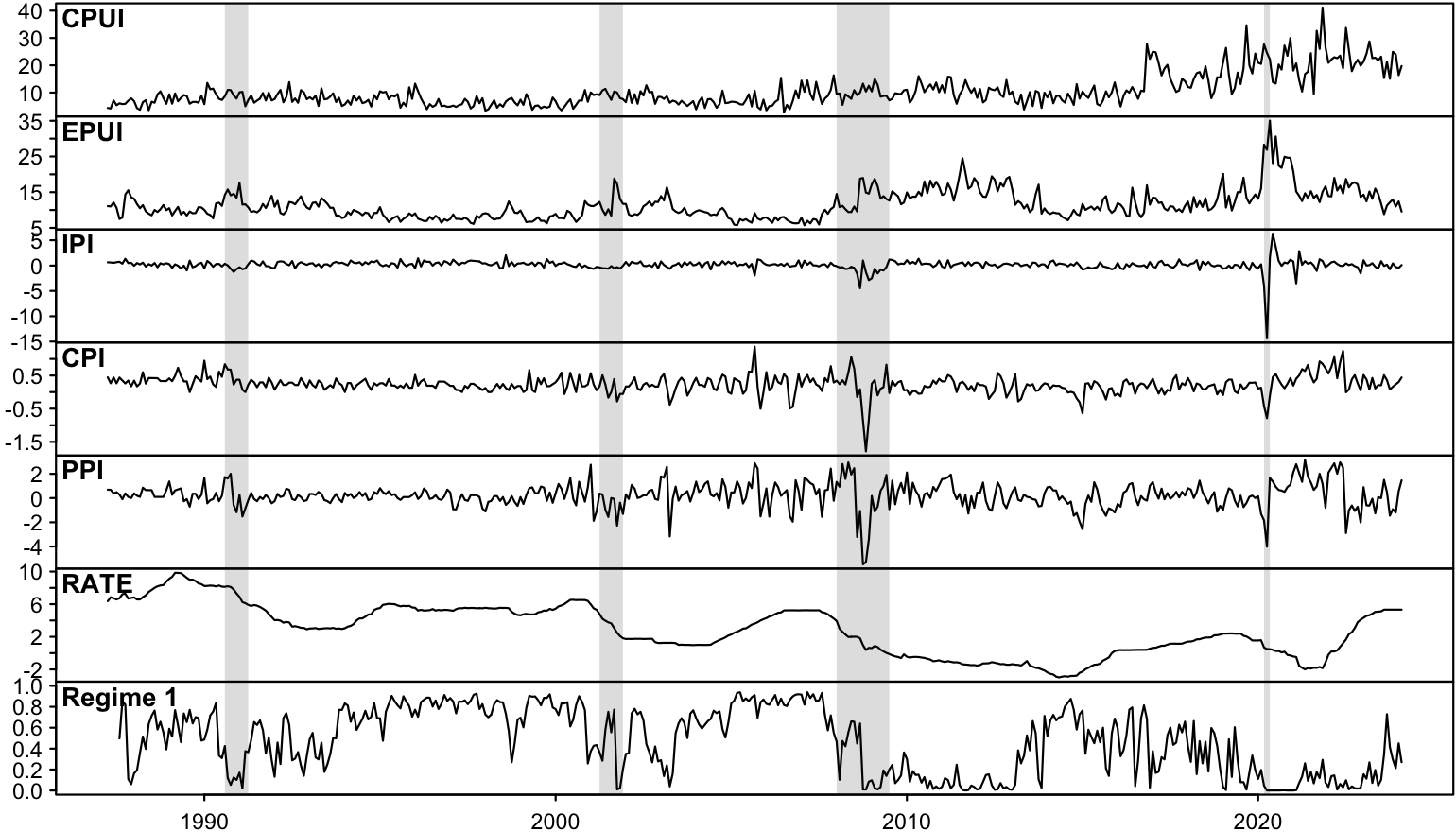
Figure 1: Monthly U.S. time series covering the period from 1987:4 to 2024:2. From top to bottom, the variables are the climate policy uncertainty index (divided by $10$), economic policy uncertainty index (divided by $10$), the log-differences of industrial production index, consumer price index, and producer price index (multiplied by $100$), and the effective federal funds rate replaced by the Wu and Xia (2016) shadow rate for the zero lower bound periods. The bottom panel shows the estimated transition weights of the first regime of the fitted two-regime fifth-order LSTVAR model. The shaded areas indicate the U.S. recessions defined by the NBER.

The series are presented in Figure 1. Both CPUI and EPUI show a generally increased level of uncertainty towards the end of the sample period, suggesting that a model accommodating shifts in the mean could be appropriate. Moreover, there is clearly variation on the volatility of the variables, so shifts the volatility regime should also be incorporated to the model.

6.2 Logistic STVAR model identified by non-Gaussianity

In order to specify the structural STVAR model (3.2)-(3.3), the transition weights and the distributions of the structural shocks need to be specified. As transition weights, we employ the popular logistic transition weights (Anderson and Vahid, 1998) given Equation (2.4) for a two-regime model. It facilitates smooth transition between the regimes depending the level of the switching variable, and it also nests the TVAR model (Tsay, 1998) as a special case when the scale parameter $\gamma$ tends to infinity. We specify the first lag of EPUI as the switching variable, thus accommodating shifts in its mean and allowing the effects of the CPU shock to vary depending the level of general economic policy uncertainty.

We assume that the structural shocks follow independent Student’s $t$ distributions, it being a fairly standard choice for modelling fat tailed data. Moreover, as the Gaussian distribution is obtained as special case of the $t$-distribution, with the degrees of freedom parameter value tending to infinity, the validity of the identifying Assumption 1 can be assessed based on the estimates of the degrees of freedom parameters. In order to maintain a reasonable number of parameters in model and avoid the problems of potentially imprecise estimates and overfitting, we assume that the autoregression matrices are constant across the regimes, i.e., employ the specification in Equation (2.6). Due to the time-varying intercepts and impact matrices, the model is still fairly general, allowing for shifts in the mean, volatility, and impact responses of the variables to the shocks.

Our two-regime logistic STVAR (LSTVAR) model then writes

$$\begin{aligned} y_{t}&=\sum_{i=1}^{p}A_{i}y_{t-i}+(1-\alpha_{2,t})(\phi_{1,0}+B_{1}e_{t})+[1+\exp\{-\gamma(y_{2t-1}-c)\}]^{-1}(\phi_{2,0}+B_{2}e_{t}),\\ e_{t}&\sim IID(0,I_{d},\nu),\end{aligned}$$ (6.1)

where $c$ is the location parameter, $\gamma>0$ is the scale parameter, $y_{2t-1}$ is the lagged EPUI, the structural shocks $e_{t}=(e_{1t},...,e_{dt})$ follow independent $t$-distributions with zero mean and unit variance, and $\nu=(\nu_{1},...,\nu_{d})$ contains the degrees of freedom parameters of the structural shocks. Finally, we select the autoregressive order $p=5$ for our model based on AIC.

The estimates of the transition weights of Regime 1 are presented in the bottom panel of Figure 1. They show that Regime 1 dominates in the periods of low economic policy uncertainty, whereas Regime 2 conversely dominates in the periods of high economic policy uncertainty. The location parameter estimate is $\hat{c}=9.80$ and the scale parameter estimate is $\hat{\gamma}=1.00$. Since the sample mean EPUI over our sample period is $11.48$, Regime 2 starts dominating roughly when EPUI surpasses its mean, and based on the small estimate of the scale parameter, the transitions between the regimes are smooth. Therefore, we label Regime 1 as the low economic policy uncertainty (EPU) regime and Regime 2 as the high EPU regime.

The estimates of the degrees of freedom parameters are small, $\hat{\nu}=(3.86,5.54,2.94,2.61,2.02,2.23)$, and therefore none of the shocks to be close to Gaussian, suggesting that Assumption 1 is satisfied. Then, we checked whether our model satisfies the stationarity condition of Theorem 1 by computing an upper bound for the joint spectral radius of the matrices $\boldsymbol{A}_{m}$ (4.2), $m=1,2$, using the JSR toolbox (Jungers, 2023) in MATLAB. The obtained upper bounds is $0.98$, which is strictly smaller than one, implying that our model satisfies Assumption 2 and is ergodic stationary by Theorem 1.

To assess the adequacy of our model, we utilize residual based model diagnostics to examine how well our model captures the autocorrelation structure, conditional heteroskedasticity, and distribution of the data. To that end, we plot several diagnostic figures, which are presented and discussed in more detail in Appendix A.6. The diagnostic figures show that our model captures the autocorrelation structure of the data reasonably well, but there is a large correlation coefficient in the crosscorrelation functions between two of the residual series. Also conditional heteroskedasticity is somewhat reasonably well captured, although there are a few relatively large correlation coefficients in the auto- and crosscorrelation functions of squared standardized residuals. The marginal distributions of the series are also reasonably well captured, but the distributions of two of the residual series are somewhat asymmetric. Nonetheless, in our view, the overall adequacy of our model is reasonable enough for impulse responses analysis. The estimates and model diagnostics are based on the final selected model after labelling the CPU shock as described in Section 6.3.

6.3 Labelling the CPU shock

The shocks of our structural LSTVAR model (6.1) are readily identified by Proposition 2. However, labelling the shocks requires external information. Moreover, due to the problem of weak identification discussed in Section 3.5, we should choose among the practically equally well fitting local solutions the solution that facilitates labelling the shock of interest to the same columns of the impact matrix in all of the regimes.

To estimates of $B_{1}$ and $B_{2}$ for the local solution with the highest obtained log-likelihood are the following:

$$\small\begin{aligned} &\hat{B}_{1}=\begin{bmatrix}\phantom{-}2.31&\phantom{-}1.31&\phantom{-}0.59&\phantom{-}0.52&\phantom{-}0.39&\phantom{-}0.24\\ \phantom{-}0.21&\phantom{-}6.50&\phantom{-}0.06&\phantom{-}0.49&\phantom{-}0.50&\phantom{-}0.48\\ -0.05&\phantom{-}0.53&\phantom{-}0.06&-0.08&-0.53&\phantom{-}0.04\\ -0.04&\phantom{-}0.07&\phantom{-}0.23&\phantom{-}0.01&\phantom{-}0.02&\phantom{-}0.08\\ -0.02&\phantom{-}0.32&\phantom{-}0.51&-0.59&\phantom{-}0.10&\phantom{-}0.20\\ -0.01&-0.09&-0.01&-0.01&\phantom{-}0.00&\phantom{-}0.19\\ \end{bmatrix},\\ &\hat{B}_{2}=\begin{bmatrix}\phantom{-}4.22&\phantom{-}1.59&\phantom{-}0.11&-0.27&-0.34&-0.21\\ \phantom{-}0.48&\phantom{-}1.30&\phantom{-}0.57&-0.08&-2.43&-0.57\\ \phantom{-}0.08&-3.90&\phantom{-}0.05&-0.07&-0.11&-0.09\\ \phantom{-}0.02&-0.17&\phantom{-}0.08&\phantom{-}0.23&\phantom{-}0.03&\phantom{-}0.01\\ \phantom{-}0.00&-0.56&\phantom{-}1.22&\phantom{-}0.50&\phantom{-}0.21&\phantom{-}0.05\\ \phantom{-}0.01&\phantom{-}0.00&-0.01&\phantom{-}0.02&-0.02&\phantom{-}0.34\\ \end{bmatrix},\end{aligned}$$ (6.2)

where the ordering of the variables is $y_{t}=(\text{CPUI}_{t},\text{EPUI}_{t},\text{IPI}_{t},\text{CPI}_{t},\text{PPI}_{t},\text{RATE}_{t})$, and the ordering and signs of the columns of $B_{1}$ and $B_{2}$ are fixed by normalizing the entries in the first row of $\hat{B_{1}}$ to be positive and in a decreasing order.

In terms of labelling the CPU shock based on the impact responses of the variables in the estimates of $B_{1}$ and $B_{2}$, there are several properties that are reasonable to expect from it. First, since the CPU shock is the shock to CPUI, the impact response of CPUI should be substantial, and it should have the same sign in $B_{1}$ and $B_{2}$. Second, as CPU contributes to the overall economic policy uncertainty, EPUI should increase or at least not significantly decrease in response to a positive CPU shock. The effects of the CPU shock on IPI can be more ambiguous. On the one hand, increased uncertainty about future climate policy can postpone investments and thereby decrease production. On the other hand, some of the firms anticipating future restrictive policies may accelerate production to preempt higher future costs. Anticipation of stricter regulations may also drive some of the firms investing towards future technologies, as proactive adaptation to anticipated climate policies may gain a competitive advantage. The effects of the CPU shock on the price level can be indirect or less immediate, translated through the effects on the aggregate demand, the production costs, or the level of production. The relationship between the CPU shock and the interest rate may also not be a direct one, as the Fed may not directly react to increased uncertainty but counteracts the economic impacts of the shock when they are observed.

Based on the estimates of $B_{1}$ in Equation (6.2), the only variable that moves substantially at impact in response to the first shock is CPUI, and the first shock has also clearly the highest impact effect on CPUI. The first shock also moves EPUI to the same direction with CPUI, in line with increased CPU contributing to the general level of economic policy uncertainty. Also the second shock moves CPUI significantly at impact, but it moves EPUI much more, so since CPUI and EPUI vary in the same scale, it does not appear to be a plausible CPU shock candidate. Therefore, the fist shock seems to be most reasonable candidate as the CPU shock. The estimates of $B_{2}$ in Equation (6.2) show that the first shock substantially moves CPUI at impact, while the response of CPUI to the other shocks is clearly smaller. Importantly, the sign of the responses of CPUI to the first shock is the same as in $\hat{B}_{1}$. Moreover, the first shock moves EPUI to the same direction with CPUI, thus, in line with what can be expected from a CPU shock. Overall, the first shock seems to be the most plausible CPU shock candidate, and hence, we deem it as the CPU shock. Since we labelled the CPUI shock in the local solution that obtained the highest likelihood, there is no need to consider other local solutions incorporating practically equal fit and mostly very similar estimates but different ordering and signs of the columns of $B_{2}$ (see Section 3.5).

6.4 Generalized impulse response functions

The effects of the structural shocks in our structural LSTVAR model may depend on the initial values as well as on the sign and size of the shock, which makes the conventional way of calculating impulse responses unsuitable. Therefore, we consider the general impulse reponse function (GIRF) (Koop et al., 1996) that accommodates such features and is defined as

$$\text{GIRF}(h,\delta_{i},\mathcal{F}_{t-1})=\text{E}[y_{t+h}|\delta_{i},\mathcal{F}_{t-1}]-\text{E}[y_{t+h}|\mathcal{F}_{t-1}],$$ (6.3)

where $h$ is the horizon. The first term on the right side of (6.3) is the expected realization of the process at time $t+h$ conditionally on a structural shock of sign and size $\delta_{i}\in\mathbb{R}$ in the $i$th element of $e_{t}$ at time $t$ and the previous observations. The latter term on the right side is the expected realization of the process conditionally on the previous observations only. The GIRF thus expresses the expected difference in the future outcomes when the structural shock of sign and size $\delta_{i}$ in the $i$th element hits the system at time $t$ as opposed to all shocks being random. The generalized impulse response functions also facilitate tracking the effects of the shock on the transition weights $\alpha_{m,t}$, $m=1,...,M$, by replacing $y_{t+h}$ with $\alpha_{m,t}$ on the right side of Equation (6.3).

As our structural LSTVAR model has a $p$-step Markov property, conditioning on (the $\sigma$-algebra generated by) the $p$ previous observations $\boldsymbol{y}_{t-1}=(y_{t-1},...,y_{t-p})$ is effectively the same as conditioning on $\mathcal{F}_{t-1}$ at the time $t$ and later. In order to study state dependence of the effects of the CPU shock, we obtain the histories $\boldsymbol{y}_{t-1}=(y_{t-1},...,y_{t-p})$ from low EPU and high EPU regimes separately. Specifically, for each regime, we take all of the length $p$ histories in the data that imply transition weights larger than $0.75$ for the given regime. For low EPU regime, there are $112$ such histories and for high EPU regime there are $202$. Then, we calculate the GIRF for each these length $p$ histories and take the sample mean to obtain a point estimate for the GIRF conditional on dominance of the given regime, whereas taking sample quantiles gives confidence intervals that reflect uncertainty about the initial state of the economy within the dominating regime. This way the GIRFs estimates the effects of the CPU shock in times of low EPU and high EPU in a way that reflects the observed data. Our Monte Carlo algorithm for computing the GIRF is similar to the one described in Lanne and Virolainen (2024), Appendix B.

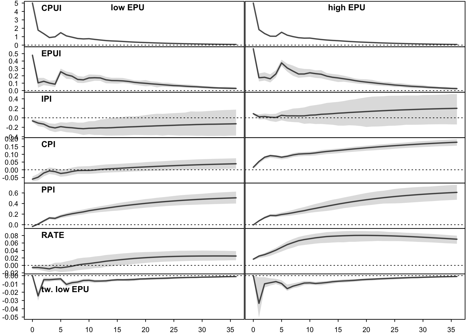
Figure 2: Generalized impulse response functions to the identified CPU shock $h=0,1,....,36$ months ahead. From top to bottom, the responses of CPUI, EPUI, IPI, CPI, PPI, the interest rate variable, and transition weights of Regime 1 are depicted in each row. The responses of IPI, CPI, and PPI are accumulated to ($100\times$)log-levels. The left column shows the responses to a positive one-standard-error CPU shock with initial values from Regime 1, whereas the right column shows the responses with initial values from Regime 2. All GIRFs have been scaled so that the instantaneous increase in CPUI is $5$. The shaded areas depict the $95\%$ confidence intervals that reflect uncertainty about the initial state of the economy within the regime.

The GIRFs to a one-standard-error positive CPU shock are presented in Figure 2. We also computed the GIRFs for two-standard-error and negative CPU shocks, but the responses were similar to the positive one-standard-error shock (after adjusting for the different sign or size), so they are not presented for brevity. The responses of CPUI and EPUI follow similar patterns during times of low and high EPU, with CPUI responding substantially and EPU more weakly, but the responses of the rest of the variables are different.

When the level of general economic policy uncertainty is low, production deceases, but when the level of EPU is high, production increases slightly. This observation could possibly be explained as follows. When EPU is low, firms may have a clearer view on the economic environment and afford to adopt a wait-and-see approach, postponing investments until the uncertainty resolves, thus, reducing production. On the other hand, when EPU is high, firms are already operating in a more unpredictable environment, with a new shock on CPU adding to the existing challenges but not fundamentally changing the level of general economic policy uncertainty. In such scenarios, firms might proceed with investments that had already been planned or accelerate production to hedge against multiple types of uncertainties. This could include ramping up production in sectors less likely to be immediately affected by the potential new regulations, or investing in a broader range of technologies to mitigate the impact of any single policy change. High levels uncertainty may also lead firms to capitalize on short term opportunities to maximize returns before any potential restrictive climate policies take effect.

Consumer prices decrease at first and then slightly increase when the level of EPU is low, while consumer prices increase more significantly when EPU is high. A possible explanation for the short-term decrease in consumer prices is a reduced consumer demand caused by postponed consumption in anticipation of new future policies leading to lower prices or greener alternatives. Consumption might be postponed also in the fear of increased maintenance and operation costs of certain products like gasoline vehicles. This effect on consumer prices can be more pronounced when overall economic policy uncertainty is low, because consumers might not feel as pressured by other economic concerns, and thus respond more directly to the climate policy uncertainty. In times of high EPU, consumer prices increase more substantially possibly because firms anticipating potential future regulations start adapting their operations proactively to meet the potential new regulations or to mitigate policy risk, increasing the production costs. When the overall economic policy uncertainty is high, firms might also have a more defence stance and pass more of the increased production costs to the consumers.

Producer prices increase permanently in times of both low and high EPU, possibly driven by anticipatory market adjustments to potential future costs of commodities. The effects of the CPU shock on the interest rate are quite small but seem consistent relative to the responses of the other variables. In particular, the interest rate increases as price increase, and the response is stronger during high EPU when the response of prices is also stronger. Finally, in both of the regimes, transition weights of the low EPU regime slightly decrease, which is expected as a positive CPU shock increases EPUI and thereby induces a shift towards the high EPU regime.

7 Conclusions

Linear structural vector autoregressive models can be identified statistically by non-Gaussianity without imposing restrictions on the model if the shocks are mutually independent and at most one of them is Gaussian (Lanne et al., 2017). We have shown that this result extends to structural threshold and smooth transition vector autoregressive models incorporating a time-varying impact matrix defined as a weighted sum of the impact matrices of the regimes. The weights of the impact matrices are the transition weights of the regimes, which we assume to be either exogenous or, for a $p$th order model, functions of the preceding $p$ observations. Thus, the types of transition weights typically used in macroeconomic applications are accommodated. The identification is often weak with respect to the ordering and signs of the columns of the impact matrices of the some of the regimes (after adjusting the parameter values), and an incorrect ordering or signs of the columns results in impulse response functions that do not estimate the effects of the intended shock but of a linear combination of the structural shocks. Therefore, we proposed a procedure to facilitate reliable labelling of the shocks by making use of short-run sign restrictions, which can be also be combined with testable economic zero restrictions and other types of information.

In addition to discussing the identification of the shocks, we have presented a sufficient condition for establishing stationarity, ergodicity, and mixing properties of our structural STVAR model. Stationarity is not, however, required for applicability of our identification results. We also discussed the estimation of the model parameters by the method maximum likelihood in case of independent Student’s $t$ shocks. The introduced methods have been implemented to the accompanying R package sstvars (Virolainen, 2024). Note that while this paper focuses in TVAR and STVAR models, our identification results directly extend to many other nonlinear SVAR models as well. This includes models incorporating discrete regime switches, such Markov-Switching VAR models and mixture VAR models, and more generally models whose impact matrix can be defined as a weighted sum of the impact matrices of the regimes and the time $t$ weights are known at the time $t$.

Our empirical application studied the macroeconomic effects of climate policy uncertainty shocks and considered a monthly U.S. data from 1987:4 to 2024:2. As a measure of climate policy uncertainty, we employed the CPU index (Gavriilidis, 2021) constructed based on the amount of newspaper coverage on climate policy uncertainty topic. We fitted a two-regime logistic STVAR model (Anderson and Vahid, 1998) using the first lag of the economic policy uncertainty index (Baker et al., 2016) as the switching variable and allowing for smooth transitions in the intercept parameters as well as in the impact matrix. We found that a positive CPU shock decreases production in times of low economic policy uncertainty, while production slightly increases in times of high economic policy uncertainty. Consumer prices, in turn, increase more significantly when the level of economic policy uncertainty is high than when it is low. Our results are, therefore, somewhat contrary to Gavriilidis et al. (2023), who found a positive CPU decreasing real activity and increasing prices, thus, transmitting to the U.S. economy as a supply shock.

Appendix A Proofs

A.1 Proof of Lemma 1

We start by showing that for all $\alpha_{1,t},...,\alpha_{M,t}$, the matrix $B_{y,t}=\sum_{m=1}^{M}\alpha_{m,t}B_{m}$ is invertible almost everywhere in $[B_{1}:...:B_{M}]\in\mathbb{R}^{d\times dM}$. First, note that by the constraints $\sum_{m=1}\alpha_{m,t}=1$ and $\alpha_{m,t}\geq 0$, $m=1,...,M$, we have $\alpha_{m,t}>0$ for some $m$ for all $t$. Therefore, for all $\alpha_{1,t},...,\alpha_{M,t}$, there exists invertible matrices $B_{1},...,B_{M}$ such that $B_{y,t}$ is invertible. The set of points $[B_{1}:...:B_{M}]\in\mathbb{R}^{d\times dM}$ (or equally $(vec(B_{1}),...,vec(B_{M}))\in\mathbb{R}^{Md^{2}}$) for which $B_{y,t}$ is singular is $S_{t}\equiv\{(vec(B_{1}),...,vec(B_{M})\in\mathbb{R}^{Md^{2}}|\det(\sum_{m=1}^{M}\alpha_{m,t}B_{m})=0\}$. Since the determinant of a matrix is polynomial in the entries of that matrix and the entries of $\sum_{m=1}^{M}\alpha_{m,t}B_{m}$ are linear combinations of the entries of $B_{1},...,B_{M}$, it follows that the determinant of $\sum_{m=1}^{M}\alpha_{m,t}B_{m}$ is a polynomial in the entries of $B_{1},...,B_{M}$. Denote this polynomial as $P_{t}(B_{1},...,B_{M})\equiv\det(\sum_{m=1}^{M}\alpha_{m,t}B_{m})$. Note that whenever $\alpha_{m,t}=0$, the impact matrices $B_{m}$ of the corresponding regimes drop out from $P_{t}(B_{1},...,B_{M})$, but in this case $P_{t}(B_{1},...,B_{M})$ can still be interpreted as a polynomial in the entries of $B_{1},...,B_{M}$ with the multipliers of the dropped entries being zero.

It then follows from Implicit function theorem that in the points $B^{0}=(vec(B_{1,0}),...,vec(B_{M,0}))\in\mathbb{R}^{Md^{2}}$ where the gradient of $P_{t}(B_{1},...,B_{M})$ is nonzero, the set $S_{t}$ is an $Md^{2}-1$-dimensional manifold locally in a neighbourhood of $B^{0}$. Because this argument applies at all points $B^{0}$ where the gradient of $P_{t}(B_{1},...,B_{M})$ is nonzero, it follows that the set $S_{t}$ is an $Md^{2}-1$-dimensional manifold in regions where this condition holds. Therefore, the Lebesque measure of the set $S_{t}$ is zero in $\mathbb{R}^{Md^{2}}$ in the region where the gradient of $P_{t}(B_{1},...,B_{M})$ is nonzero. On the other hand, by Sard’s theorem (Sard, 1994), the set of points where the gradient of $P_{t}(B_{1},...,B_{M})$ is zero has a Lebesgue measure zero in $\mathbb{R}^{Md^{2}}$. Since the union of two sets with a Lebesgue measure zero has a Lebesgue measure zero, these results can be combined to conclude that the $S_{t}$ has a Lebesgue measure zero in $\mathbb{R}^{Md^{2}}$.

Finally, note that since the above result holds for all $\alpha_{1,t},...,\alpha_{M,t}$, the set $S_{t}$ has a Lebesgue measure zero in $\mathbb{R}^{Md^{2}}$ for each $t$. Hence, the union $\cup_{t=1}^{\infty}S_{t}$ is a union of a countable number of measure zero sets and thus itself has a Lebesgue measure zero. It follows that the matrix $B_{y,t}$ is invertible for all $t$ almost everywhere in $[B_{1}:...:B_{M}]\in\mathbb{R}^{d\times dM}$, concluding the proof.∎

A.2 Proof of Lemma 2

For most parts, our proof is similar to the proof of Proposition 1 in Lanne et al. (2017) making use of results from independent component analysis (Comon, 1994). First, note that from Equation (3.2), we can rewrite the model as

$$y_{t}-\phi_{t}-\boldsymbol{A}_{t}\boldsymbol{y}_{t-1}=B_{y,t}e_{t},$$ (A.1)

where $\phi_{t}\equiv\sum_{m=1}^{M}\alpha_{m,t}\phi_{m,0}$ $(d\times 1)$, $\boldsymbol{A}_{t}\equiv[A_{y,t,1}:...:A_{y,t,p}]$ $(d\times dp)$, and $A_{y,t,i}\equiv\sum_{m=1}^{M}\alpha_{m,t}A_{m,i}$ contain the time-varying AR coefficients, and $\boldsymbol{y}_{t-1}=(y_{t-1},...,y_{t-p})$. Then, suppose Equation (A.1) holds also for some other coefficients, impact matrix, and shocks $\tilde{\phi}_{t},\tilde{\boldsymbol{A}}_{t}$, $\tilde{B}_{y,t}$, and $\tilde{e}_{t}$, i.e., $y_{t}-\tilde{\phi}_{t}-\tilde{\boldsymbol{A}}_{t}\boldsymbol{y}_{t-1}=\tilde{B}_{y,t}\tilde{e}_{t}$. By subtracting this identify from (A.1), we obtain

$$\tilde{\phi}_{t}-\phi_{t}+(\tilde{\boldsymbol{A}}_{t}-\boldsymbol{A}_{t})\boldsymbol{y}_{t-1} =B_{y,t}e_{t}-\tilde{B}_{y,t}\tilde{e}_{t}$$ (A.2)

Taking conditional expectation conditional on $\mathcal{F}_{t-1}$ gives

$$\tilde{\phi}_{t}-\phi_{t}+(\tilde{\boldsymbol{A}}_{t}-\boldsymbol{A}_{t})\boldsymbol{y}_{t-1} =0,$$ (A.3)

as $E[B_{y,t}e_{t}|\mathcal{F}_{t-1}]=E[\tilde{B}_{y,t}\tilde{e}_{t}|\mathcal{F}_{t-1}]=0$ (by $e_{t}\perp\!\!\!\!\perp\mathcal{F}_{t-1}$ and $E[e_{t}]=0$). By substituting this back to (A.2), we get

$$B_{y,t}e_{t}=\tilde{B}_{y,t}\tilde{e}_{t}.$$ (A.4)

Since $B_{y,t}$ is invertible almost everywhere in $[B_{1}:...:B_{M}]\in\mathbb{R}^{d\times dM}$ by Lemma 1, we can solve $e_{t}$ as $e_{t}=C\tilde{e}_{t}$, where $C=B_{y,t}^{-1}\tilde{B}_{y,t}$ is $\mathcal{F}_{t-1}$-measurable. By Assumption 1, the random variables $\tilde{e}_{1t},...,\tilde{e}_{dt}$ are mutually independent and at most one of them is Gaussian. Also the random variables $e_{1t},...,e_{dt}$ are mutually independent and at most one of them is Gaussian. Therefore, conditionally on $\mathcal{F}_{t-1}$, by Darmois-Skitovich theorem (Lemma A.1 in Lanne et al., 2017), at most on column of $C$ may contain more than one nonzero element. Suppose, say, the $k$th column of $C$ has at least two nonzero elements, $c_{ik}$ and $c_{jk}$, $i\neq j$. Then, $e_{it}=c_{ik}\tilde{e}_{kt}+\sum_{l=1,l\neq k}^{d}c_{il}\tilde{e}_{lt}$ and $e_{jt}=c_{jk}\tilde{e}_{kt}+\sum_{l=1,l\neq k}^{d}c_{jl}\tilde{e}_{lt}$ with $\tilde{e}_{kt}$ Gaussian (by Darmois-Skitovich theorem). This implies that $E[e_{it}e_{jt}]=c_{ik}c_{jk}\neq 0$ (since $E[\tilde{e}_{kt}^{2}]=1$) so that $e_{it}$ and $e_{jt}$ are not independent, which is a contradiction. Hence, each column of $C$ has at most one nonzero element.

Now, from the invertibility of $C$ it follows that each column of $C$ as exactly one nonzero element, and for the same reason, also that each row of $C$ has exactly one nonzero element. Therefore, there exists a permutation matrix $P$ and a diagonal matrix $D=\text{diag}(d_{1},...,d_{d})$ with nonzero diagonal elements such that $C=DP$. Together with $C=B_{y,t}^{-1}\tilde{B}_{y,t}$ this implies that $\tilde{B}_{y,t}=B_{y,t}DP$ and $\tilde{e}_{t}=P^{\prime}D^{-1}e_{t}$, concluding that $B_{y,t}$ is unique up to ordering of its columns and multiplying each column by a constant.

To complete proof, it needs to be shown that the diagonal elements of $D$ are either $1$ or $-1$. By the normalization of the unit variances of $e_{t}$ and $\tilde{e}_{t}$, $\text{Cov}(\tilde{e}_{t}|\mathcal{F}_{t-1})=\text{Cov}(Ce_{t}|\mathcal{F}_{t-1})=I_{d}$, which is equivalent to $C\text{Cov}(e_{t}|\mathcal{F}_{t-1})C^{\prime}=I_{d}$ and thereby $CC^{\prime}=I_{d}$. By substituting $C=DP$ to this expression, we obtain $DPP^{\prime}D^{\prime}=I_{d}$ and by the orthogonality of permutation matrix $DD^{\prime}=I_{d}$. That is, $d_{ii}^{2}=1$ for all $i=1,...,d$, so $d_{ii}=\pm 1$. Since diagonal elements of $D$ are, hence, either $1$ or $-1$, it follows that $B_{y,t}$ is unique up to ordering of its columns and changing all signs in a column almost everywhere in $[B_{1}:...:B_{M}]\in\mathbb{R}^{d\times dM}$.∎

A.3 Proof of Proposition 1

We start by showing that under the conditions of Proposition 1, the ordering and signs of the columns of $B_{y,t}$ are fixed for all $t$ in the sense that reordering or changing the signs of the columns of $B_{y,t}$ at any $t$ would lead to model that is not observationally equivalent with the original one. Specifically, we say that two models are observational equivalent if and only if their joint densities are equal. After that, we combine this result with Lemma 2 to show that $B_{1},...,B_{M}$ are uniquely identified.

Condition (a) readily fixes the signs of the columns of $B_{1},...,B_{M}$, so it suffices the check that under Conditions (c) and (b), changing the ordering of the columns of any of $B_{2},...,B_{M}$ would change the joint density of the model. Suppose the observed time series is $y_{t-p+1},...,y_{0},y_{1},...,y_{T}$ and denote $Y_{T}=(y_{T},...,y_{0})$. Conditional on the initial values $y_{t-p+1},...,y_{0}$, the joint density of the model is

$$f_{Y}(Y_{T})=\prod_{t=1}^{T}\left(|\det(B_{t})|^{-1}\prod_{i=1}^{d}d_{e_{i}}(I_{d,i}^{\prime}B_{y,t}^{-1}(y_{t}-\mu_{t});0,1,\nu_{i})\right),$$ (A.5)

where $I_{d,i}$ is the $i$th column of the $d$-dimensional identity matrix and $d_{e_{i}}(\cdot;0,1,\nu_{i})$ is the density function the $i$th shock. At each $t$, $B_{y,t}=B_{m}$ for the regime $m$ with $\alpha_{m,t}=1$, implying the that the density (A.5) can be expressed as

$$f_{Y}(Y_{T};B_{1},...,B_{M}) =\prod_{m=1}^{M}\prod_{t\in\mathcal{T}_{m}}f_{y}(y_{t}-\mu_{t};B_{m}),\ \ \text{and}$$ (A.6)

$$f_{y}(y_{t}-\mu_{t};B_{m}) =|\det(B_{m})|^{-1}\prod_{i=1}^{d}d_{e_{i}}(I_{d,i}^{\prime}B_{m}^{-1}(y_{t}-\mu_{t});0,1,\nu_{i}),$$ (A.7)

where $\mathcal{T}_{m}$, $m=1,...,M$, is the (nonempty) set of time indices that satisfy $\alpha_{m,t}=1$ for the regime $m$, and the dependence of the density functions $f_{Y}(\cdot;B_{1},...,B_{M})$ and $f_{y}(\cdot;B_{m})$ on the impact matrices $B_{1},...,B_{M}$ is now made explicit in the notation (but its dependence on the other parameters is omitted).

Denote by $\boldsymbol{\tau}_{m}=(\tau_{m1},...,\tau_{md})$ the permutation $\tau_{m1},...,\tau_{md}$ of the columns of $B_{m}$, and denote by $B_{m}(\boldsymbol{\tau}_{m})$ the impact matrix $B_{m}$ corresponding to the permutation $\boldsymbol{\tau}_{m}$ of its columns. Then, consider the permutations $\boldsymbol{\tau}_{1},\boldsymbol{\tau}_{2},...,\boldsymbol{\tau}_{M}$ and $\boldsymbol{\tau}_{1},\tilde{\boldsymbol{\tau}}_{2},...,\tilde{\boldsymbol{\tau}}_{M}$. By the invertibility of $B_{m}$, none of the entries in $B_{m}^{-1}(y_{t}-\mu_{t})$ are equal to each other almost everywhere in $Y_{T}\in\mathbb{R}^{T}$. Since reordering the columns of $B_{m}$ reorders the rows of $B_{m}^{-1}$, it then follows that if $\tilde{\boldsymbol{\tau}}_{m}\neq\boldsymbol{\tau}_{m}$, some of the entries in $B_{m}^{-1}(\boldsymbol{\tau}_{m})(y_{t}-\mu_{t})$ and $B_{m}^{-1}(\tilde{\boldsymbol{\tau}}_{m})(y_{t}-\mu_{t})$ are in a different order. Moreover, as $|\det(B_{m})|$ is invariant to the ordering of the columns of $B_{m}$, it follows from this and Condition (c) that, almost everywhere in $Y_{T}\in\mathbb{R}^{T}$, $f_{y}(y_{t}-\mu_{t};B_{m}(\boldsymbol{\tau}_{m}))\neq f_{y}(y_{t}-\mu_{t};B_{m}(\tilde{\boldsymbol{\tau}}_{m}))$ whenever $\tilde{\boldsymbol{\tau}}_{m}\neq\boldsymbol{\tau}_{m}$.

Therefore, as the shocks and thereby $y_{t}$ follows a continuous distribution, we have

$$\prod_{t\in\mathcal{T}_{m}}f_{y}(y_{t}-\mu_{t};B_{m}(\boldsymbol{\tau}_{m}))\neq\prod_{t\in\mathcal{T}_{m}}f_{y}(y_{t}-\mu_{t};B_{m}(\tilde{\boldsymbol{\tau}}_{m})),$$ (A.8)

and thus also

$$f_{Y}(Y_{T};B_{1}(\boldsymbol{\tau}_{1}),B_{2}(\boldsymbol{\tau}_{2}),...,B_{M}(\boldsymbol{\tau}_{M}))\neq f_{Y}(Y_{T};B_{1}(\boldsymbol{\tau}_{1}),B_{2}(\tilde{\boldsymbol{\tau}}_{2})...,B_{M}(\tilde{\boldsymbol{\tau}}_{M}))$$ (A.9)

almost everywhere in $Y_{T}\in\mathbb{R}^{T}$ whenever $\tilde{\boldsymbol{\tau}}_{m}\neq\boldsymbol{\tau}_{m}$ for any $m=2,...,M$. Since the this result holds almost everywhere in $Y_{T}\in\mathbb{R}^{T}$, and $B_{y,t}$ is here invertible for all invertible $B_{1},...,B_{M}$, the result holds almost everywhere in $Y_{T}\in\mathbb{R}^{T}$.

Finally, by Lemma 2, $B_{y,t}$ is identified up to ordering and signs of its columns at each $t$. Thus, each impact matrix $B_{1},...,B_{M}$ of the regimes is identified up to ordering signs of its columns. Under the conditions of Proposition 1, the signs of the columns of $B_{1},...,B_{M}$ and the ordering of the columns $B_{1}$ are directly fixed. Moreover, by the above discussion, different permutations of the columns of any of $B_{2},...,B_{M}$ lead to different values of the joint density function of the model almost everywhere in $Y_{T}\in\mathbb{R}^{T}$, i.e., to models that are not observationally equivalent. Thus, only models corresponding to the same permutations of the columns of $B_{2},...,B_{M}$ are observationally equivalent, implying that the matrices $B_{1},...,B_{M}$ are uniquely identified almost everywhere in $Y_{T}\in\mathbb{R}^{T}$.∎

A.4 Proof of Proposition 2

To proof consists of two parts. First, we show that almost everywhere in $[B_{1}:\cdots:B_{M}]\in\mathbb{R}^{d\times dM}$, if the ordering and signs of the columns of $B_{1}$ is fixed, changing ordering or signs of the columns of any of $B_{2},...,B_{M}$ leads to an impact impact matrix $B_{y,t}$ that cannot, at all $t$, be obtained by reordering or changing the signs of the columns of the original impact matrix. In other words, we show that fixing the ordering signs of the columns of $B_{1}$ effectively fixes the ordering and signs of the columns of $B_{2},...,B_{M}$ and thereby of $B_{y,t}$. Then, we make use of this result together with the result of Lemma 2 (that $B_{y,t}$ is identified up ordering and signs of its columns at each $t$) to show that the matrices $B_{1},...,B_{M}$ are uniquely identified almost everywhere in $[B_{1}:\cdots:B_{M}]\in\mathbb{R}^{d\times dM}$.

Denote by $\boldsymbol{\tau}_{m}=(\tau_{m1},...,\tau_{md})$ the permutation $\tau_{m1},...,\tau_{md}$ and $\boldsymbol{\iota}_{m}=(\iota_{m1},...,\iota_{md})$ the sign changes $\iota_{m1},...,\iota_{md}$ of the columns of $B_{m}$, respectively. Moreover, denote by $B_{m}(\boldsymbol{\tau}_{m},\boldsymbol{\iota}_{m})$ the invertible impact matrix $B_{m}$ corresponding to the permutation $\boldsymbol{\tau}_{m}$ and sign changes $\boldsymbol{\iota}_{m}$ of its columns. Then, consider the permutations $\boldsymbol{\tau}_{1},\boldsymbol{\tau}_{2},...,\boldsymbol{\tau}_{M}$ and $\boldsymbol{\tau}_{1},\tilde{\boldsymbol{\tau}}_{2},...,\tilde{\boldsymbol{\tau}}_{M}$ as well the sign changes $\boldsymbol{\iota}_{1},\boldsymbol{\iota}_{2},...,\boldsymbol{\iota}_{M}$ and $\boldsymbol{\iota}_{1},\tilde{\boldsymbol{\iota}}_{2},...,\tilde{\boldsymbol{\iota}}_{M}$. We start by showing that $B_{y,t}(\boldsymbol{\tau},\boldsymbol{\iota})\equiv\alpha_{1,t}B_{1}(\boldsymbol{\tau}_{1},\boldsymbol{\iota}_{1})+\sum_{m=2}^{M}\alpha_{m,t}B_{m}(\boldsymbol{\tau}_{m},\boldsymbol{\iota}_{m})$ cannot be obtained by reordering or changing the signs of the columns of $B_{y,t}(\tilde{\boldsymbol{\tau}},\tilde{\boldsymbol{\iota}})\equiv\alpha_{m,t}B_{1}(\boldsymbol{\tau}_{1},\boldsymbol{\iota}_{1})+\sum_{m=2}^{M}\alpha_{m,t}B_{m}(\tilde{\boldsymbol{\tau}}_{m},\tilde{\boldsymbol{\iota}}_{m})$ almost everywhere in $[B_{1},...,B_{M}]\in\mathbb{R}^{d\times Md}$ whenever $\boldsymbol{\tau}_{m}\neq\tilde{\boldsymbol{\tau}}_{m}$ or $\boldsymbol{\iota}_{m}\neq\tilde{\boldsymbol{\iota}}_{m}$ for any $m=2,...,M$.

At each time period $t$, the impact matrix $B_{y,t}(\tilde{\boldsymbol{\tau}},\tilde{\boldsymbol{\iota}})$ is obtained by reordering or changing the signs of the columns of $B_{y,t}(\boldsymbol{\tau},\boldsymbol{\iota})$ if and only if

$$\alpha_{1,t}B_{1}(\boldsymbol{\tau}_{1},\boldsymbol{\iota}_{1})+\sum_{m=2}^{M}\alpha_{m,t}B_{m}(\boldsymbol{\tau}_{m},\boldsymbol{\iota}_{m})=(\alpha_{m,t}B_{1}(\boldsymbol{\tau}_{1},\boldsymbol{\iota}_{1})+\sum_{m=2}^{M}\alpha_{m,t}B_{m}(\tilde{\boldsymbol{\tau}}_{m},\tilde{\boldsymbol{\iota}}_{m}))D_{t}P_{t}$$ (A.10)

for some $(d\times d)$ diagonal matrix $D_{t}$ with $\pm 1$ diagonal elements and some $(d\times d)$ permutation matrix $P_{t}$ (that may vary in time). Rearranging the above equation gives

$$\sum_{m=2}^{M}\alpha_{m,t}(B_{m}(\boldsymbol{\tau}_{m},\boldsymbol{\iota}_{m})-B_{m}(\tilde{\boldsymbol{\tau}}_{m},\tilde{\boldsymbol{\iota}}_{m})D_{t}P_{t})=-\alpha_{1,t}B_{1}(\boldsymbol{\tau}_{1},\boldsymbol{\iota}_{1})(I_{d}-D_{t}P_{t}).$$ (A.11)

Suppose first $D_{t}P_{t}=I_{d}$. Equation (A.12) then simplifies to

$$\sum_{m=2}^{M}\alpha_{m,t}(B_{m}(\boldsymbol{\tau}_{m},\boldsymbol{\iota}_{m})-B_{m}(\tilde{\boldsymbol{\tau}}_{m},\tilde{\boldsymbol{\iota}}_{m}))=0.$$ (A.12)

By Condition (B), the vector $(\alpha_{1,t},...,\alpha_{M,t})$ takes a value for some $t$ such that none of its entries is zero. At each such time period $t$, Equation (A.12) is nontrivial, as by invertibility, none of the columns of $B_{m}$ can be equal or negatives of each other. Hence, the set of matrices $B_{2},...,B_{M}$ that satisfy Equation (A.12) forms a subspace in $\mathbb{R}^{d\times d(M-1)}$ with the dimension of this subspace being less than $(M-1)d^{2}$, as it must satisfy a nontrivial linear equation. Consequently, the set of matrices $B_{2},...,B_{M}$ that satisfy Equation (A.12) has a Lebesgue measure zero in $[B_{2}:\cdots:B_{M}]\in\mathbb{R}^{d\times d(M-1)}$, implying that the set of matrices $B_{1},...,B_{M}$ satisfying this equation have a Lebesgue measure zero in $[B_{1}:\cdots:B_{M}]\in\mathbb{R}^{d\times Md}$.

Suppose then $D_{t}P_{t}\neq I_{d}$ and denote the left side of Equation (A.11) as $C_{t}\in\mathbb{R}^{d\times d}$. By Condition (B), the vector $(\alpha_{1,t},...,\alpha_{M,t})$ takes a value for some $t$ such that none of its entries is zero. At each such time period $t$, the right side of Equation (A.11) is nonzero, thus, implying that also $C_{t}$ is not a matrix zeros. Equation (A.11) is thereby nontrivial and can be expressed as

$$B_{1}(\boldsymbol{\tau}_{1},\boldsymbol{\iota}_{1})(I_{d}-D_{t}P_{t})=\alpha_{1,t}^{-1}C_{t}$$ (A.13)

The set of matrices $B_{1}$ that satisfy Equation (A.13) forms a subspace in $\mathbb{R}^{d\times d}$ with the dimension of this subspace being less than $d^{2}$, as it must satisfy a nontrivial linear equation. It follows that the set of matrices $B_{1}$ that satisfy Equation (A.13) has Lebesgue measure zero on $\mathbb{R}^{d\times d}$, and therefore, the set of matrices $B_{1},...,B_{M}$ that satisfy Equation (A.13) has a Lebesgue measure zero in $[B_{1}:\cdots B_{M}]\in\mathbb{R}^{d\times Md}$.

By the above discussion, for any single transformation $D_{t}P_{t}$ of $B_{y,t}$, the set of matrices $B_{1},...,B_{M}$ that satisfy Equation (A.11) for any time period when all the entries of $(\alpha_{1,t},...,\alpha_{M,t})$ are nonzero has a Lebesgue measure zero in $[B_{1}:\cdots B_{M}]\in\mathbb{R}^{d\times Md}$. Since there exists a finite number of such transformations and a countable union of measure zero sets has a measure zero, it follows that the set of matrices $B_{1},...,B_{M}$ that satisfy Equation (A.12) for all $t$ has a Lebesgue measure zero in $[B_{1}:\cdots:B_{M}]\in\mathbb{R}^{d\times Md}$.

Next, we make use of the above result together with Lemma 2 to show that $B_{1},...,B_{M}$ are uniquely identified $[B_{1}:\cdots:B_{M}]\in\mathbb{R}^{d\times Md}$. Consider the impact matrix $B_{y,t}=\sum_{m=1}^{M}\alpha_{m,t}B_{m}$ with some invertible $(d\times d)$ matrices $B_{1},...,B_{M}$. By Lemma 2, $B_{y,t}$ is uniquely identified at each $t$ up to ordering and signs of its columns (conditionally on $\mathcal{F}_{t-1}$). Since the ordering and signs of the columns of $B_{1}$ are fixed (Condition (A)), we then obtain from the above results that almost everywhere in $[B_{1}:...:B_{M}]\in\mathbb{R}^{d\times dM}$, reordering or changing the signs of the columns of $B_{2},...,B_{M}$ would, at some $t$, lead to an impact matrix that cannot obtained by reordering or changing the signs of the columns of $B_{y,t}$. Hence, reordering or changing the signs of the columns of any of $B_{2},...,B_{M}$ would lead to a model that is not observationally equivalent with the original one. The ordering and signs of the columns of $B_{1},...,B_{M}$ are thereby effectively fixed under Condition (A), implying that the ordering and signs of the columns of $B_{y,t}$ are also fixed for all $t$ (almost everywhere in $[B_{1}:...:B_{M}]\in\mathbb{R}^{d\times dM}$). Thus, $B_{y,t}$ is uniquely identified at all $t$.

Since $B_{y,t}$ is uniquely identified and two models are observationally equivalent if and only if they are observationally equivalent at all $t$, a unique identification of the matrices $B_{1},...,B_{M}$ is achieved if an impact matrix that is identical to $B_{y,t}$ for all $t$ cannot be obtained with any other invertible $(d\times d)$ matrices $\tilde{B}_{1},...,\tilde{B}_{M}$. Suppose an impact matrix identical to $B_{y,t}$ for all $t$ is obtained with some invertible $(d\times d)$ matrices $\tilde{B}_{1},...,\tilde{B}_{M}$. Then,

$$\sum_{m=1}^{M}\alpha_{m,t}(B_{m}-\tilde{B}_{m})=0,$$ (A.14)

for all $t$.

Denote the $ij$th element of $\tilde{B}_{m}$ as $\tilde{b}_{ij}^{(m)}$. At each $t$, Equation (A.14) then defines a system of linear equations involving $d^{2}$ equations and $Md^{2}$ variables $\tilde{b}_{ij}^{(m)}$, $j,i=1,...,d$, $m=1,...,M$. The weights $\alpha_{m,t}$ are treated as constant multipliers here, as they are predetermined at each $t$ (by $\mathcal{F}_{t-1}$-measurability or nonrandomness), and the parameters in $B_{1},...,B_{M}$ are also constants here. If $\alpha_{m,t}=0$ for some regimes $m$, the corresponding variables in $\tilde{B}_{m}$ drop out of the system of equations, however.

Under Condition (C), the vector $(\alpha_{1,t},...,\alpha_{M,t})$ and all its subvectors $(\alpha_{n_{1},t},...,\alpha_{n_{M^{\circ}},t})$, $n_{l}\in\mathbb{M^{\circ}}$, $\mathbb{M^{\circ}}\subset\{1,...,M\}$, where $M^{\circ}\geq 2$ denotes the number of elements in $\mathbb{M^{\circ}}$, take at least $M+1$ linearly independent values (plus one accounting for transition weights that equal to zero). Therefore, Equation (A.14) defined together for all $t$ defines a system of linear equations involving $Md^{2}$ variables and at least $Md^{2}$ linearly independent equations. Moreover, as $(\alpha_{1,t},...,\alpha_{M,t})$ and all its subvectors take at least $M+1$ linearly independent values, each variable $\tilde{b}_{ij}^{(m)}$ appears in at least $M$ linearly independent the equations. Thus, there exists at most one solution to this system of linear equations. Since one solution is $\tilde{B}_{m}=B_{m}$ for all $m=1,...,M$, this is the unique solution, concluding that the matrices $B_{1},...,B_{M}$ are uniquely identified almost everywehere in $[B_{1}:\cdots:B_{M}]\in\mathbb{R}^{d\times dM}$.∎

A.5 Proof of Theorem 1

Saikkonen (2008) establishes stationarity, ergodicity, and mixing properties of a STVEC model by making use of the theory of Markov chains. Kheifets and Saikkonen (2020), in turn, show that the results of Saikkonen (2008) are applicable to their STVAR model, as it can be obtained as a special case of the STVEC model of Saikkonen (2008). However, the results of Saikkonen (2008) and Kheifets and Saikkonen (2020) are not directly applicable to our structural STVAR model, because our model defines the conditional covariance matrix differently to the STVEC model of Saikkonen (2008) and STVAR model of Kheifets and Saikkonen (2020). Hence, certain steps need to be taken show the applicability of the results of Saikkonen (2008) to our structural STVAR model.

Note that by Assumption 2(II), Assumption 1 in Saikkonen (2008) is satisfied. Moreover, by the constraint $\sum_{m=1}^{M}\alpha_{m,t}=1$, Assumption 2(a) in Saikkonen (2008) satisfied, and as we assume that the set $\text{l}_{2}$ in Saikkonen (2008) is an empty set, also Assumption 2(b) is satisfied. Consequently, Condition (10) in Saikkonen (2008) is satisfied and by our Assumption 2(I) also Condition (19). The difference of our setup to the conditions of Theorem 1 of Saikkonen (2008) is that our STVAR model specifies the conditional covariance matrix differently to the STVEC model defined in Equation (8) of Saikkonen (2008).

Besides the conditional covariance matrix, our structural STVAR model defined in Equations (3.2) and (3.3) is obtained from the stochastic process $z_{t}$ defined in Equation (17) (or equally (15)) of Saikkonen (2008) as follows. First, we assume that the number of unit roots in the model is zero, so $n=r$ in Saikkonen (2008). Consequently, $z_{t}=y_{t}$ and, in the definition of the matrix $J$ defined above Equation (17) of Saikkonen (2008), $\beta=c=I_{d}$ (see Saikkonen, 2008, Note 2). The matrix $J$ is thereby nonsingular, and following Kheifets and Saikkonen (2020), we can choose the matrix $S$ in Equation (17) to be the inverse of $J^{\prime}$. Second, we assume the transition functions $h_{s}(S^{\prime}JZ_{t-1},\eta_{t})$ of Saikkonen (2008) are independent of the random variable $\eta_{t}$. Hence, the transition functions are functions of $Z_{t-1}=(y_{t-1},...,y_{t-p})$, and we can write $h_{s}(S^{\prime}JZ_{t-1},\eta_{t})=\alpha_{m,t}$. Using the notation of this paper, the first term on the right side of Equation (17) in Saikkonen (2008) then reduces to $\sum_{m=1}^{M}\alpha_{m,t}\sum_{i=1}^{p}A_{m,i}y_{t-i}$. Third, assume the set $\text{l}_{2}$ is empty, which implies that the second term on the right side of Equation (17), defined in Equation (11) of Saikkonen (2008), reduces to $\sum_{m=1}^{M}\alpha_{m,t}\phi_{m,0}$ (with the notation of this paper).

That is, the first two terms on the right side of Equation (17) in Saikkonen (2008), reduce to the first term on the right hand side of Equation (3.2) defining our structural STVAR model. The third term on the right side of Equation (17) in Saikkonen (2008), however, reduces to $(\sum_{m=1}^{M}\alpha_{m,t}\Omega_{m})^{1/2}e_{t}$, where $\Omega_{1},...,\Omega_{M}$ are positive definite $(d\times d)$ covariance matrices of the regimes. This is different to the second term of Equation (3.2), which takes the form $\sum_{m=1}^{M}\alpha_{m,t}B_{m}e_{t}$ when the impact matrix (3.3) is substituted to it. Nonetheless, it turns out that with only slight modifications, the proof of Theorem 1 in Saikkonen (2008) applies to our model as well.

The conditional covariance matrix is relevant in only a few places in the proof of Theorem 1 in Saikkonen (2008). Firstly, on page 312, Saikkonen (2008) makes use of the positive definiteness of the conditional covariance matrix $H(S^{\prime}JZ_{t-1})$ (or $\sum_{m=1}^{M}\alpha_{m,t}\Omega_{m}$ in our notation) to conclude that the smallest eigenvalue of $H(S^{\prime}Jx)$, $x\in\mathbb{R}^{dp}$, is bounded away from zero in compact subsets of $\mathbb{R}^{dp}$. Saikkonen (2008) argues that thereby by Theorem 2.2(ii) of Cline and Phu (1998), the Markov chain $Z_{t}$ is an irreducible and aperiodic T-chain on $\mathbb{R}^{dp}$, which is then used to conclude further results. Concerning our model, note that by Lemma 1, $B_{y,t}$ is invertible for all $t$ almost everywhere in $[B_{1}:...:B_{M}]\in\mathbb{R}^{d\times dM}$, implying that the conditional covariance matrix $B_{y,t}(\boldsymbol{y}_{t-1})B_{y,t}(\boldsymbol{y}_{t-1})^{\prime}$ is positive definite, where the dependence of the conditional covariance matrix on the $(dp\times 1)$ random vector $\boldsymbol{y}_{t-1}=(y_{t-1},...,y_{t-p})$ is made explicit in the notation. Hence, the smallest eigenvalue of $B_{y,t}(x)B_{y,t}(x)^{\prime}$, $x\in\mathbb{R}^{dp}$, is bounded away from zero in compact subsets of $\mathbb{R}^{dp}$. It follows from this, Equation (3.2), and the invertibility of $B_{y,t}$ that we can apply Theorem 2.2(ii) of Cline and Phu (1998) to conclude that the Markov chain $\boldsymbol{y}_{t}$ is an irreducible and aperiodic T-chain on $\mathbb{R}^{dp}$, similarly to the process $Z_{t-1}$ in Saikkonen (2008).

Secondly, the conditional covariance matrix appears in the proof of Saikkonen (2008) on page 313, where Saikkonen (2008) shows that an appropriate version of Condition (15.3) of Meyn and Tweedie (1993, p. 358) is satisfied. To show that this condition holds for our model, we need to show that an appropriate version of Equation (A.5) in Saikkonen (2008) holds for our model, i.e., that the term $E[\sup_{A\in\mathcal{A}^{j}}||AB_{y,t}(x)e_{t}||^{2}]$, where $j$ is a positive integer, is bounded from above by a finite real number.

Similarly to Saikkonen (2008, p. 313), clearly,

$$\sup\{||A||:A\in\cup_{j=1}^{N}\mathcal{A}^{j}\}<c,$$ (A.15)

where $||\cdot||$ is Eucledian norm, $N$ is a positive integer, and $c$ a finite real number. Hence, because $B_{y,t}(x)$ is a constant here, by Jensen’s inequality and submultiplicativity of norms, we have

$$E\left[\sup_{A\in\mathcal{A}^{j}}||AB_{y,t}(x)e_{t}||^{2}\right]\leq\sup_{A\in\mathcal{A}^{j}}||A||^{2}||B_{y,t}(x)||^{2}E[||e_{t}||]^{2},$$ (A.16)

where the right side is bounded from above by some finite constant (by (A.15) and the finite second moment of $e_{t}$ given by Assumption 1). Thus, an appropriate version of Equation (A.5) in Saikkonen (2008) holds for our model. Since the rest of the proof of Theorem 1 in Saikkonen (2008) thereby applies to our model as well, this concludes the proof.∎

A.6 Details on the empirical application

The ML estimation of the models, residual diagnostics, and estimation of the GIRFS are carried out with the R package sstvars (Virolainen, 2024) to which the methods introduced in this paper have been implemented. The R package sstvars also contains the dataset studied in the empirical application to facilitate reproduction of our results. In estimation, we consider only solutions that can deemed local maximums of the log-likelihood function.

In the below residual based model diagnostics, we have not labelled the residual series by any of the variables, because identification with respect to the ordering of the columns of $B_{2}$ is weak (see Section 3.5). Then, changing the ordering of the columns changes the ordering of the variables in the density function $t_{1}(I_{d,i}^{\prime}B_{y,t}^{-1}(y_{t}-\mu_{t});0,1,\nu_{i})$, thus, changing the ordering of the residuals in this regime. The residual time series can, therefore, be labelled only for the variables whose structural shocks have been labelled. Since we labelled the CPU shock as the first shock in Section 6.3, the first residual series constitutes the residuals of CPUI.

To study whether our model adequately captures the autocorrelation structure of the data, we depict the sample autocorrelation functions (ACF) and cross-correlation functions (CCF) of the residuals for the first $24$ lags in Figure 3. As the figure shows, there is not much autocorrelation left in the residuals, but there is a particularly large correlation coefficient (CC) in the first lag of the CCFs between the fourth and fifth residual series. There are also some moderate sized CCFs in the ACFs of the residual series, but these are not particularly large. Since rest of the CCs are reasonable, our LSTVAR model seems to capture the autocorrelation structure of the data reasonably well.

In order to study the model’s adequacy to capture the conditional heteroskedasticity of the data, we depict the sample ACFs and CCFs of squared standardized residuals for the first $24$ lags in Figure 4. The figure shows that there are several moderate and relative large CCs in the ACFs and CCFs of some of the residual series. Thus, there is some but not particularly severe inadequacies in terms of capturing the conditional heteroskedasticity.

The series of standardized residuals, presented in the top panels of Figure 5, also show some remaining heteroskedasticity and several outliers, many of which are accommodated by the heavy tailed $t$-distributions. Finally, the quantile-quantile-plots based on the independent $t$-distributions with mean zero, variance one, and degrees of freedom given by the degrees of freedom parameter estimate are presented in the bottom panel of Figure 1. They show that the marginal distributions of the series are relatively well captured, although the distributions of two of the residual series are slightly asymmetric. Nonetheless, in our view, the overall adequacy of the model seems relatively reasonable.

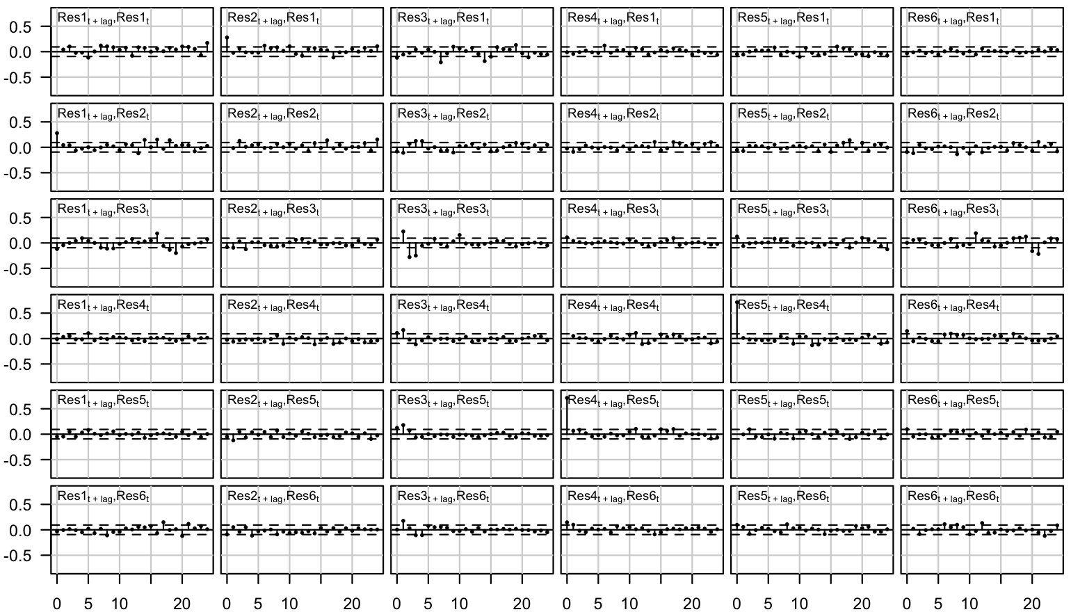
Figure 3: Auto- and crosscorrelation functions of the residuals of the fitted two-regime fifth-order LSTVAR model for the lags $0,1,...,24$. The lag zero autocorrelation coefficients are omitted, as they are one by convention. The dashed lines are the $95\%$ bounds $\pm 1.96/\sqrt{T}$ for autocorrelations of IID observations.

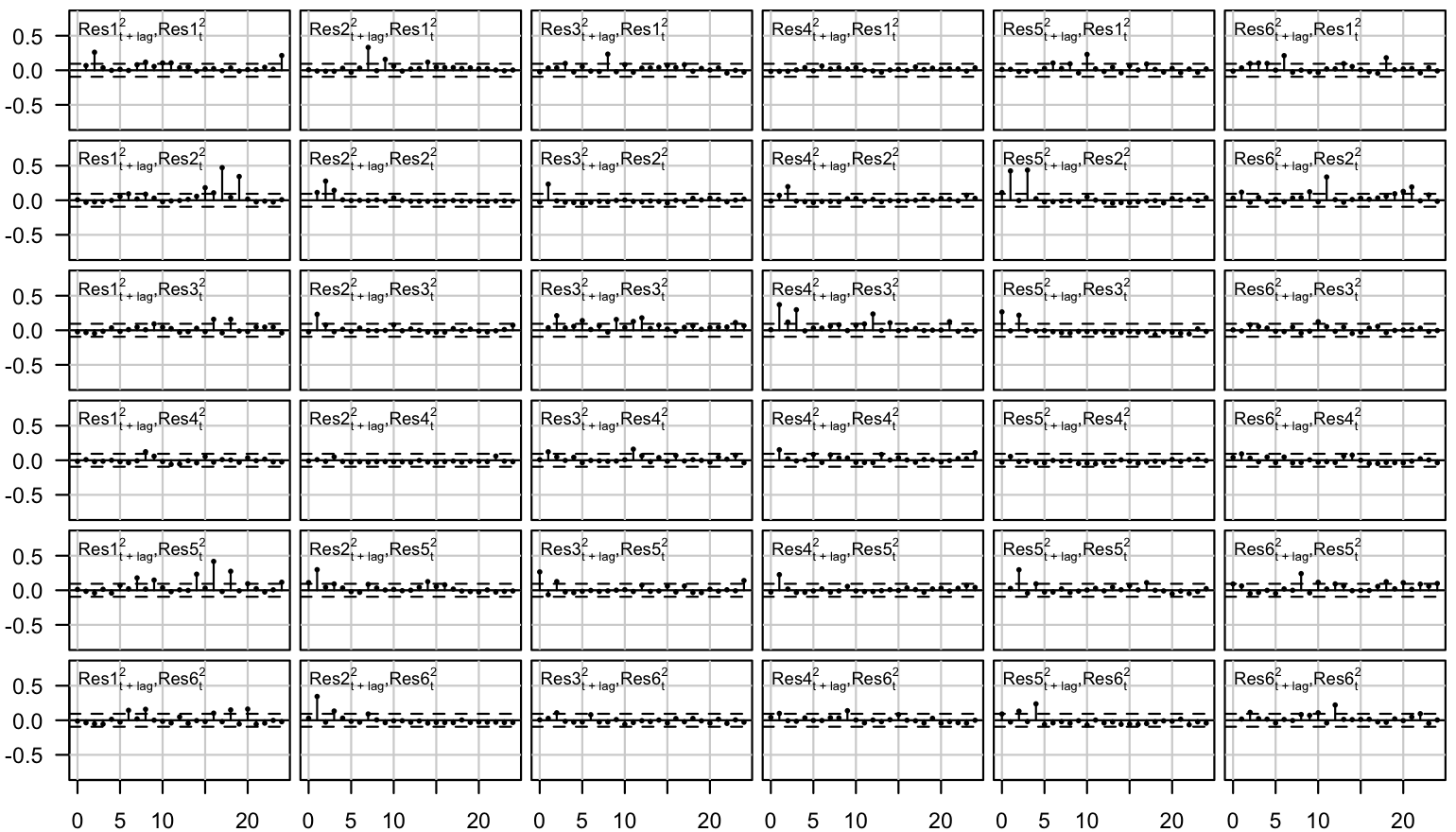
Figure 4: Auto- and crosscorrelation functions of the squared standardized residuals of the fitted two-regime fifth-order LSTVAR model for the lags $0,1,...,24$. The lag zero autocorrelation coefficients are omitted, as they are one by convention. The dashed lines are the $95\%$ bounds $\pm 1.96/\sqrt{T}$ for autocorrelations of IID observations.

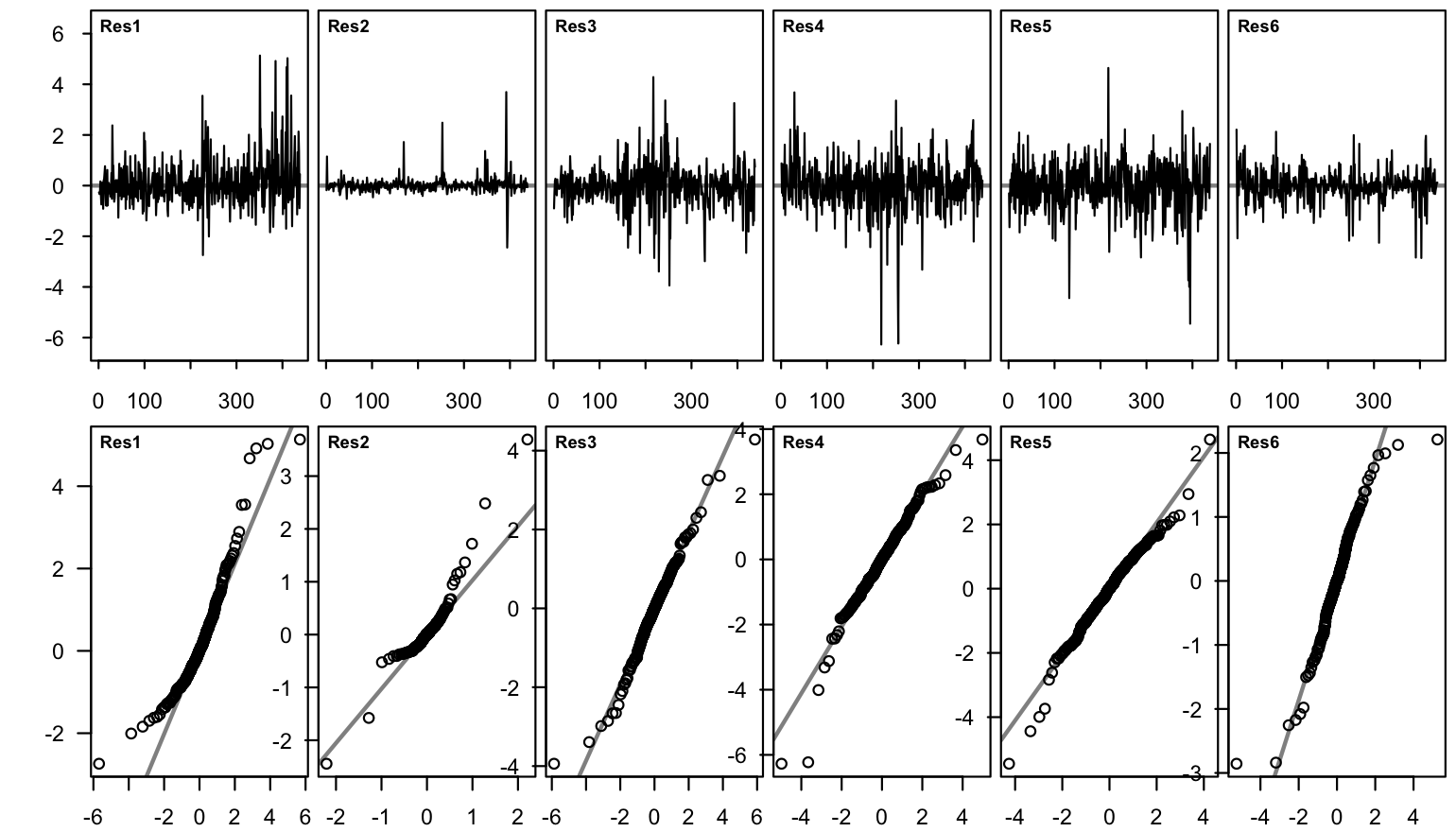
Figure 5: Standardized residual time series and quantile-quantile-plots of the fitted two-regime fifth-order LSTVAR model. The quantile-quantile plots are based on $t$–distributions with zero mean, variance one, and degrees of freedom given by the ML estimate of the degrees of freedom parameter.

References

- Anderson and Vahid (1998) Anderson H., Vahid F. (1998). “Testing multiple equation systems for common nonlinear components.” Journal of Econometrics, 84(1), 1–36.
- Anttonen et al. (forthcoming) Anttonen J., Lanne M., Luoto J. (forthcoming). “Statistically identified structural var model with potentially skewed and fat-tailed errors.” Journal of Applied Econometrics.
- Bacchiocchi and Fanelli (2015) Bacchiocchi E., Fanelli L. (2015). “Identification in structural vector autoregressive models with structural changes, with an application to us monetary policy.” Oxford Bulletin of Economics and Statistics, 77(6), 761–779.
- Baker et al. (2016) Baker S., Bloom N., Davis S. (2016). “Measuring economic policy uncertainty.” Quarterly Journal of Economics, 131(4), 1593–1636.
- Chang and Blondel (2013) Chang C.-T., Blondel V. (2013). “An experimental study of approximation algorithms for the joint spectral radius.” Numerical Algorithms, 64, 181–202.
- Cline and Phu (1998) Cline D. B., Phu H.-M. H. (1998). “Verifying irreducibility and continuity of a nonlinear time series.” Statistics & Probability Letters, 40(2), 139–148.
- Comon (1994) Comon P. (1994). “Independent component analysis, a new concept?” Signal Processing, 36(3), 287–314.
- Fong et al. (2007) Fong P., Li W., Yau C., Wong C. (2007). “On a mixture vector autoregressive model.” The Canadian Journal of Statistics, 35(1), 135–150.
- Fried et al. (2021) Fried S., Novan K., Peterman W. (2021). “The macro effects of climate policy uncertainty.” Finance and Economic Discussion Series.
- Gavriilidis (2021) Gavriilidis K. (2021). “Measuring climate policy uncertainty. Available at SSRN: https://ssrn.com/abstract=3847388.”
- Gavriilidis et al. (2023) Gavriilidis K., Känzig D., Stock J. (2023). “The macroeconomic effects of climate policy uncertainty.” Unpublished working paper.
- Gripenberg (1996) Gripenberg G. (1996). “Computing the joint spectral radius.” Linear algebra and its applications, 234, 43–60.
- Hubrich and Teräsvirta (2013) Hubrich K., Teräsvirta T. (2013). “Thresholds and smooth transitions in vector autoregressive models.” CREATES Research Paper 2013-18, Aarhus University.
- Jungers (2023) Jungers R. (2023). “The JSR toolbox (https://www.mathworks.com/matlabcentral/fileexchange/33202-the-jsr-toolbox), matlab central file exchange.”
- Kheifets and Saikkonen (2020) Kheifets I., Saikkonen P. (2020). “Stationarity and ergodicity of vector STAR models.” Econometric Reviews, 39(407–414), 1311–1324.
- Kilian and Lütkepohl (2017) Kilian L., Lütkepohl H. (2017). “Structural vector autoregressive analysis.” 1st edition. Cambridge University Press, Cambridge.
- Koop et al. (1996) Koop G., Pesaran M., Potter S. (1996). “Impulse response analysis in nonlinear multivariate models.” Journal of Econometrics, 74(1), 119–147.
- Krolzig (1997) Krolzig H.-M. (1997). “Markov-switching vector autoregressions - modelling, statistical inference, and application to business cycle analysis.” In H Dawid, A Kleine (eds.), Lecture Notes in Economcia and Mathematical Systems, volume 454, chapter 1, pp. 6–28. Springer Berlin, Heidelberg, Berlin.
- Lanne et al. (2023) Lanne M., Liu K., Luoto J. (2023). “Identifying structural vector autoregression via leptokurtic economic shocks.” Journal of Business & Economic Statistics, 41(4), 1341–1351.
- Lanne and Luoto (2021) Lanne M., Luoto J. (2021). “Gmm estimation of non-gaussian structural vector autoregression.” Journal of Business & Economic Statistics, 39(1), 69–81.
- Lanne et al. (2010) Lanne M., Lütkepohl H., Maciejowska K. (2010). “Structural vector autoregressions with Markov switching.” Journal of Economic Dynamics and Control, 34(2), 121–131.
- Lanne et al. (2017) Lanne M., Meitz M., Saikkonen P. (2017). “Identification and estimation of non-Gaussian structural vector autoregressions.” Journal of Econometrics, 196(2), 288–304.
- Lanne and Virolainen (2024) Lanne M., Virolainen S. (2024). “A Gaussian smooth transition vector autoregressive model: An application to the macroeconomic effects of severe weather shocks.” Unpublished working paper, available as arXiv:2403.14216.
- Lütkepohl and Netšunajev (2017) Lütkepohl H., Netšunajev A. (2017). “Structural vector autoregressions with smooth transitions in variances.” Journal of Economic Dynamics & Control, 84, 43–57.
- Maxand (2020) Maxand S. (2020). “Identification of independent structural shocks in the presence of multiple gaussian components.” Econometrics and Statistics, 16, 55–68.
- Meitz et al. (2023) Meitz M., Preve D., Saikkonen P. (2023). “A mixture autoregressive model based on Student’s -distribution.” Communications in Statistics - Theory and Methods, 52(2), 499–515.
- Meyn and Tweedie (1993) Meyn S., Tweedie R. (1993). “Markov chains and stochastic stability.” 1st edition. Springer-Verlag, London.
- Morioka et al. (2021) Morioka H., Hälvä H., Hyvärinen A. (2021). “Independent innovation analysis for nonlinear vector autoregressive process.” Proceedings of Machine Learning Research, 130, 1549–1557.
- Ramey (2016) Ramey V. A. (2016). “Macroeconomic shocks and their propagation.” In JB Taylor, H Uhlig (eds.), Handbook of Macroeconomics, volume 2, chapter 2. Elsevier Science B.V.
- Rigobon (2003) Rigobon R. (2003). “Identification through heteroskedasticity.” The Review of Economics and Statistics, 85(4), 777–792.
- Saikkonen (2008) Saikkonen P. (2008). “Stability of regime switching error correction models under linear cointegration.” Econometric Theory, 24(1), 294–318.
- Sard (1994) Sard A. (1994). “The measure of the critical values of differentiable maps.” Bulletin of the Americal Mathematical Society, 48(12), 883–890.
- Tsay (1998) Tsay R. (1998). “Testing and modeling multivariate threshold models.” Journal of the American Statistical Association, 93(443), 1188–1202.
- Virolainen (2022) Virolainen S. (2022). “A mixture autoregressive model based on Gaussian and Student’s -distributions.” Studies in Nonlinear Dynamics & Econometrics, 26(4), 559–580.
- Virolainen (2024) Virolainen S. (2024). “sstvars: Toolkit for structural smooth transition vector autoregressive models.” R package version 1.0.0 available at GitHub: https://github.com/saviviro/sstvars.
- Virolainen (forthcoming) Virolainen S. (forthcoming). “A statistically identified structural vector autoregression with endogeneously switching volatility regime.” Journal of Business & Economic Statistics.
- Wu and Xia (2016) Wu J., Xia F. (2016). “Measuring the macroeconomic impact of monetary policy at the zero lower bound.” Journal of Money, Credit and Banking, 48(2-3), 253–291.