Kapitza-Inspired Stabilization of Non-Foster Circuits via Time Modulations

Abstract

With his formal analysis in 1951, the physicist Pyotr Kapitza demonstrated that an inverted pendulum with an externally vibrating base can be stable in its upper position, thus overcoming the force of gravity. Kapitza’s work is an example that an originally unstable system can become stable after a minor perturbation of its properties or initial conditions is applied. Inspired by his ideas, we show how non-Foster circuits can be stabilized with the application of external electrical vibration, i.e., time modulations. Non-Foster circuits are highly appreciated in the engineering community, since their bandwidth characteristics are not limited by passive-circuits bounds. Unfortunately, non-Foster circuits are usually unstable and they must be stabilized prior to operation. Here, we focus on the study of non-Foster $L(t)C$ circuits with time-varying inductors and time-invariant negative capacitors. We find an intrinsic connection between Kapitza’s inverted pendulum and non-Foster $L(t)C$ resonators. Moreover, we show how positive time-varying modulations of $L(t)>0$ can overcome and stabilize non-Foster negative capacitances $C<0$. These findings open up an alternative manner of stabilizing electric circuits with the use of time modulations, and lay the groundwork for application of, what we coin Vibrational Electromagnetics, in more complex media.

I Introduction

In 1951, Nobel laureate Pyotr Kapitza introduced a theory that effectively described the physics of one of the systems that physicists were unable to interpret at that time: the inverted pendulum with a vibrating base [1, 2]. The history of this problem dates back to 1908, when physicist Andrew Stephenson suggested that the upper position in a conventional pendulum could become stable with the addition of a high-frequency vibrating base with a small amplitude of vibration [3]. The addition of this external element can indeed counteract the force of gravity that pulls the pendulum downwards, causing the pendulum to swing around its upper position without falling down. An experiment of this fascinating phenomenon can be easily performed in a high school classroom nowadays, although necessary conditions for stability are not trivial and were far from clear until Kapitza’s formal analysis in 1951.

Kapitza’s approach was based on the separation of the time scales and the use of time-averaging techniques [4]. He assumed that the external vibrating base oscillates with a frequency $\Omega$ much higher compared to the natural oscillating frequency of the pendulum, $\omega_{0}\equiv\sqrt{g/l}$ ($g\approx 9.81$ m/s² is the acceleration of gravity and $l$ is the length of the pendulum). If, additionally, the amplitude of the modulation $\delta$ is small compared to the length of the pendulum $l$, perturbation techniques can be invoked to reach an approximate analytical solution. In a scenario with these characteristics, it is possible to describe the motion (i.e., the pendulum’s angle $\theta(t)$ in Fig. 1) of the inverted pendulum with a vibrating base by separating the total contribution into two main terms: the slow and fast components of $\theta(t)$ = $\theta_{s}(t)$ + $\theta_{f}(t)$ . The slow component $\theta_{s}(t)$, a low-frequency term, represents the main contribution. On the other hand, the fast component $\theta_{f}(t)$, a small-amplitude and high-frequency term, is a secondary perturbative contribution. Interestingly, the time scales of the slow and fast components are rather different. Kapitza took advantage of that to find an analytical relation between the two and obtained physically-insightful explanation to the stability problem. See the supplementary materials for some details.

Appealingly, Kapitza’s ideas have transcended the scientific community beyond their initial application in the description of the mechanics of the inverted pendulum, leading to the subject of Vibrational Mechanics. A variety of stimulations with different time scales are commonly seen in different fields of science and engineering. The overall low-frequency response of linear and, especially, nonlinear systems excited by multiple inputs may be significantly affected by weak time-varying high-frequency contributions [5, 6, 7]. This phenomenon is named as Vibrational Resonance, term originally coined by Landa and McClintock [8] when studying high-frequency nonlinear oscillators and their connection to stochastic terms. Kapitza-inspired techniques have been applied to the analysis of a wide variety of physical, electronic and biological systems, such as the Chua’s circuit [9], lasers [10], logic gates [11], energy harvesters [12], quantum wells [13], Hindmarsh-Rose neuronal systems [14], stratified media [15] or time-periodic potentials [16, 17].

Concurrently, in a completely different discipline, the field of metamaterials has recently gained renewed attention with the inclusion of temporal modulations as part of their inner structure [18, 19]. The so-called space-time or four-dimensional (4D) metamaterials are engineered structures whose mechanical or electrical properties change over space and time [20]. The use of time in material parameter variation as a new degree of freedom has allowed for innovative designs that overcome the performance of their static, time-invariant counterparts, such as magnetless non-reciprocal devices [21, 22], beamformers and beamsteerers [23, 24], frequency converters [25, 26], power combiners [27], or temporal lenses [28].

In a different context, temporal modulations have enabled an alternative scheme to produce non-Foster electronic components [29, 30, 31, 32]; namely, circuit elements that do not satisfy Foster’s reactance theorem [33]. Non-Foster circuits are active structures whose bandwidth characteristics are not limited by Bode-Fano and Carlin-La Rosa bounds [34, 35, 36]. For instance, antenna and metamaterial communities have benefited of their use to improve impedance matching performance [37]. One of the conventional methods for implementing simple non-Foster elements, such as negative resistors, inductors or capacitors, is via the negative impedance converters formed by transformers and cross-coupled transistors [38]. In fact, first patented ideas on the production of non-Foster elements date back to the 1920s and 1930s [39, 40, 41]. Unfortunately, non-Foster components are usually unstable and their stabilization is a challenging task [42, 43, 44].

In the present work, inspired by Kapitza’s ideas and the field of Vibrational Mechanics, we analyze the stability conditions of time-varying non-Foster resonators. First, we will focus on scenarios where the inductor is time modulated and the capacitor has a time-invariant negative capacitance. Then, we will show how a time modulated positive inductance $L(t)>0$ can stabilize a negative element capacitance $C<0$. This phenomenon, which may seem unexpected or counterintuitive at first, is a result of a vibrational resonance occurred in the non-Foster resonator. Moreover, we will show that the frequency of the already stabilized non-Foster resonator can be tuned over time by dynamically changing $L(t)$.

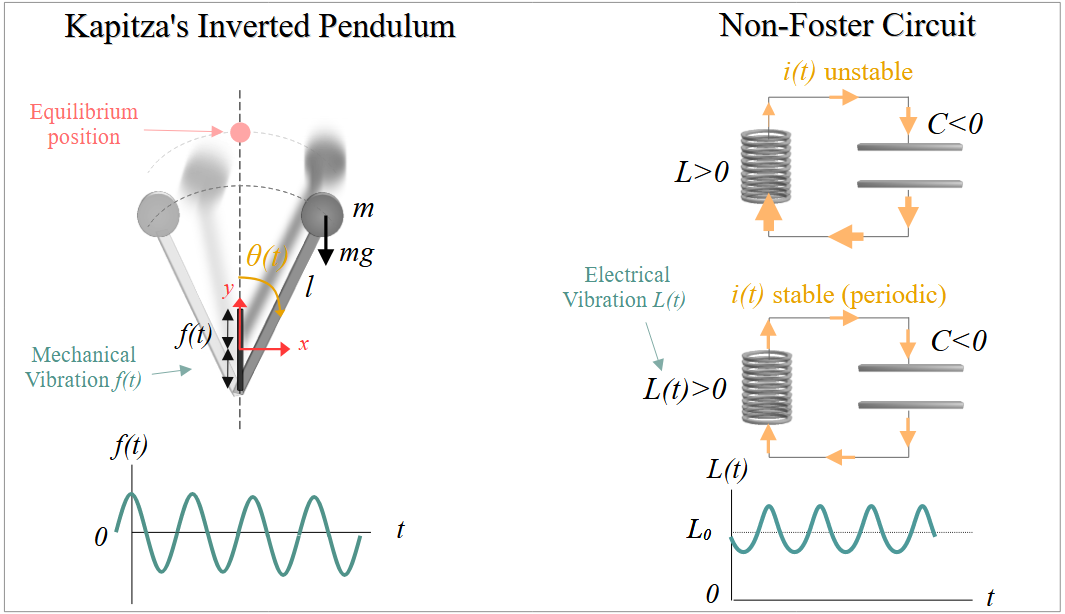
Figure 1: Connection between Kapitza’s inverted pendulum and time-modulated non-Foster circuits. Vibrational resonances appear in both systems, making them stable.

II Connection between the Non-Foster $L(t)C$ and Kapitza’s Inverted Pendulum

Let us consider the non-Foster $L(t)C$ resonator sketched in Figure 1, formed by a time-invariant negative capacitor $C<0$ and a time-varying inductor $L(t)$. In the time-invariant capacitor, the relation between voltage $v_{c}(t)$ and current $i_{c}(t)$ is given by $i_{C}(t)=C\,dv_{C}(t)/dt$. Similarly, the instantaneous relation between current $i_{L}(t)$ and voltage $v_{L}(t)$ in the time-varying inductor is given by $v_{L}(t)=d[L(t)\,i_{L}(t)]/dt$. Simple circuit analysis reveals that the differential equation that models the current in the non-Foster $L(t)C$ resonator takes the form

$$i^{\prime\prime}(t)+p(t)\,i^{\prime}(t)+q(t)\,i(t)=0\,.$$ (1)

Prime (^′) and double prime (^′′) notation indicates the first and second derivatives of the considered function. This equation is a second-order linear ordinary differential equation (ODE) with variable coefficients $p(t)$ and $q(t)$. The variable coefficients are computed as

$$p(t)\equiv\frac{2L^{\prime}(t)}{L(t)},\quad q(t)\equiv\frac{\frac{1}{C}+L^{\prime\prime}(t)}{L(t)}\,.$$ (2)

Please note that, in the absence of modulation ($\delta=0$), the governing ODE reduces to that of a conventional $LC$ circuit with time-invariant elements. In addition, it can be shown that the inclusion of loss terms via a time-invariant resistor $R$, to form a series $RL(t)C$ resonator, only affects the value of the coefficient $p(t)$, which should be simply updated to $p(t)=(2L^{\prime}(t)+R)/L(t)$. (See the Suplementary Materials.)

The fact of having variable coefficients $p(t)$ and $q(t)$ that depend not only on the applied modulating $L(t)$, but also on its first and second derivative, complicates the analysis of the circuit considerably. It also makes it difficult to draw direct relationships and analogy between the $L(t)C$ circuit and Kapitza’s inverted pendulum. Therefore, we now reduce the original ODE to an equivalent differential equation that is simpler to analyze. Given the change of variable

$$i(t)=\phi(t)\,\mathrm{e}^{-\frac{1}{2}\int_{0}^{t}p(\tau)d\tau}\,,$$ (3)

a second-order linear ODE such as eq. (1) can be transformed to the normal form [45]

$$\phi^{\prime\prime}(t)+X(t)\,\phi(t)=0\,,$$ (4)

where $X(t)\equiv q(t)-\frac{1}{2}p^{\prime}(t)-\frac{1}{4}p^{2}(t)$. For the variable coefficients $p(t)$ and $q(t)$ in eq. (2), the term $X(t)=1/[L(t)C]$ and the ODE for the new variable $\phi(t)$ takes the form

$$\phi^{\prime\prime}(t)+\frac{1}{L(t)C}\,\phi(t)=0\,.$$ (5)

In the case of $L(t)C$ resonator, the variable coefficient $p(t)$ is written as $p(t)=2L^{\prime}(t)/L(t)$, whose integral is $\int_{0}^{t}p(\tau)d\tau=2\ln[L(t)]$. Thus, $\mathrm{e}^{-\frac{1}{2}\int_{0}^{t}p(\tau)d\tau}=1/L(t)$ and

$$i(t)=\frac{\phi(t)}{L(t)}\,,$$ (6)

for a generic modulation of the inductance $L(t)$. It is worth noting that in the way eq. (6) is given, the term $\phi(t)=i(t)L(t)$ essentially represents the magnetic flux associated with the inductor.

To find the current $i(t)$ in eq. (1), we can first solve for $\phi(t)$ in eq. (5) and then reapply the change of variable $i(t)=\phi(t)/L(t)$. This way of proceeding is more convenient, since it provides us with relevant information about the stability conditions of the system. By inspecting eqs. (5) and (6), it is clear that the current $i(t)$, so the non-Foster resonator, will be stable as long as $\phi(t)$ is stable and $1/L(t)$ is bounded. Naturally, it is easier to set stability criteria for $\phi(t)$ in (5) than directly for eq. (1). Moreover, the mathematical reduction of the original ODE now shows a direct physical connection between the non-Foster $L(t)C$ and the inverted pendulum. It can be shown (See the supplementary materials) that the ODE that describes the temporal evolution of the angle $\theta(t)$ in Kapitza’s inverted pendulum is

$$\theta^{\prime\prime}(t)+\left[\alpha\Omega^{2}\cos(\Omega t)-\omega_{0}^{2}\right]\sin\left[\theta(t)\right]=0\,,$$ (7)

In eq. (7), the parameter $\alpha\equiv\delta/l$ is a dimensionless constant that relates the amplitude of the added mechanical vibration $\delta$ and the fixed length of the pendulum $l$, $\Omega$ is the angular frequency of the added mechanical vibration, and $\omega_{0}^{2}\equiv g/l$ is the square of the natural oscillation frequency of the pendulum ($g\approx 9.81$ m/$s^{2}$ is the acceleration of gravity). We note that the reduced ODE (5) in the $L(t)C$ resonator has the same exact form as the ODE (7) in Kapitza’s inverted pendulum in the case of considering small angles $\theta(t)$. Note that in the small-angle approximation, $\sin[\theta(t)]\approx\theta(t)$. In fact, it is possible to mimic the behavior of the inverted pendulum by selecting a proper modulation of the inductance $L(t)$. To do so, we have to enforce $\alpha\Omega^{2}\cos(\Omega t)-\omega_{0}^{2}=1/[L(t)C]$. Thus, the time modulation $L(t)$ that mimics the response of Kapitza’s inverted pendulum is

$$L(t)=\frac{1}{C\left[\alpha\Omega^{2}\cos(\Omega t)-\omega_{0}^{2}\right]}\,,$$ (8)

The associated current $i(t)$ is computed via eq. (6):

$$i(t)=\phi(t)\,C\left[\alpha\Omega^{2}\cos(\Omega t)-\omega_{0}^{2}\right]\,.$$ (9)

Inspection of eq. (9) reveals that the current $i(t)$ essentially represents an amplitude-modulated version of the temporal evolution of the angle in the inverted pendulum, as $\phi(t)$ effectively plays the role of $\theta(t)$.

Kapitza showed that the inverted pendulum can be stable in its upper vertical position as long as the frequency of the mechanical vibration $\Omega$ exceeds the limit value $\Omega_{\mathrm{lim}}=\sqrt{2}\omega_{0}/\alpha$, which dictates that, no matter how small the relative amplitude of the applied vibration $\alpha$ is, we can always use a frequency $\Omega>\Omega_{\mathrm{lim}}$ high enough to make the inverted pendulum stable. Same rationale applies for the non-Foster $L(t)C$ resonator. When the applied time modulation of $L(t)$ is that of eq. (8), the non-Foster resonator can become stable if the frequency of the electrical vibration $\Omega$ exceeds the limit frequency $\Omega_{\mathrm{lim}}$.

Figure 2 illustrates the stabilization of the non-Foster circuit as a result of the applied modulation frequency $\Omega$. In order to compute the current in the circuit, we extract $\phi(t)$ by numerically solving the ODE (5) and then use eq. (9) to recover $i(t)$. The relative amplitude of the modulation is chosen to be $\alpha=0.1$, a relatively small value. For this amplitude, the limit frequency that marks stability is $\Omega_{\mathrm{lim}}=\sqrt{2}\omega_{0}/0.1\approx 14.14\omega_{0}$. Above $\Omega_{\mathrm{lim}}$, the $L(t)C$ circuit will be stable. The considered initial conditions are $\phi(0)=\phi_{0}$ and $\phi^{\prime}(0)=0$, with $\phi_{0}=-0.2$. These values translate into the following initial conditions for $i(t)$: $i(0)=\phi_{0}C(\alpha\Omega^{2}-\omega_{0}^{2})$ and $i^{\prime}(0)=0$.

Figure 2(a) shows an unstable case, with $\Omega$ less than the limit frequency. Figure 2(b) shows a stable case, with $\Omega$ greater than the limit frequency. The term $\phi(t)$ is essentially a scaled version of the envelope of the current $i(t)$ flowing through the non-Foster circuit. Naturally, this can also be inferred after inspecting eq. (9). Red dotted line in Figures 2(a) and (b) represent $\phi(t)$ after normalization. In addition, please note that, when the applied modulation of $L(t)$ is that of eq. (8), the magnetic flux $\phi(t)$ would also represent the angle $\theta(t)$ in a Kapitza’s inverted pendulum. Thus, if $\phi(t)$ is stable, then the current $i(t)$ is stable too.

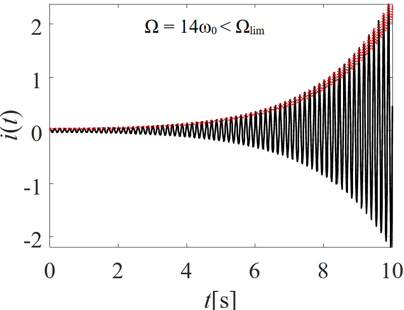
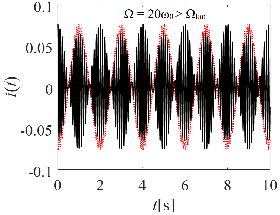
Figure 2: Current $i(t)$ in the non-Foster $L(t)C$ resonator. The modulated $L(t)$ is the one that mimics the behavior of Kapitza’s inverted pendulum [eq. (8)]. (a) Unstable case. (b) Stable case. The red dotted line represents a normalized version of $\phi(t)$. Parameters: $\alpha=0.1$, $C=-10^{-3}$ F.

III Stabilization via positive $L(t)$

In the previous section, we have shown the physical correspondence between Kapitza’s inverted pendulum and the non-Foster circuit. Moreover, we have illustrated that the non-Foster $L(t)C$ circuit can be stable if $L(t)$ is given by eq. (8) and the modulation frequency $\Omega$ exceeds Kapitza’s limit value $\Omega_{\mathrm{lim}}=\sqrt{2}\omega_{0}/\alpha$. Unfortunately, the use of (8) presents two main impracticalities. The first one is that $|L(t)|\rightarrow\infty$ at some temporal instants $t$. Nonetheless, this impracticality is probably the least important, since it is possible to take sufficiently large, but finite, values of the inductance to approximate the asymptotic behavior of $L(t)$. The second and most important impracticality of using eq. (8) is that $L(t)$ becomes negative. Actually, $L(t)$ is negative approximately half of the modulation period and positive the other half. Not only do we need a time-varying inductor to stabilize the circuit, which is not easy to put into practice, but we also need it to alternate between positive and negative inductance values, which makes it effectively impossible.

Now, the question that remains is: can we find a modulating $L(t)>0$ that avoids the use of negative and zero values? Eq. (5) leaves this possibility open. If it is possible to find a stable $\phi(t)$ for a positive-valued time-modulated inductor $L(t)$, then the current $i(t)$ (and thus the voltage) should be stable too. Finding via trial and error a non-negative expression for $L(t)$ that makes the non-Foster system stable is really inefficient. In this regard, the technique developed in [29, 32] can be helpful. The underlying idea there is that temporal modulations of a circuit element with positive values (e.g., a capacitor) allow to mimic the response of positive- or negative-valued time-invariant circuit elements. A double-negative ($L_{\mathrm{eq}}<0$ and $C<0$) non-Foster resonator is naturally stable. Thus, if a positive time-varying inductor $L(t)>0$ behaves, equivalently, as a negative-valued time-invariant inductor $L_{\mathrm{eq}}<0$, then the time-varying non-Foster resonator will be stable.

In order to ensure that the time-varying inductor $L(t)$ behaves exactly the same as an equivalent (negative-valued) time-invariant inductor $L_{\mathrm{eq}}$, voltages and current flowing through both terminals have to be identical ($d[L(t)i_{L}(t)]/dt=L_{\mathrm{eq}}\,d[i_{L\mathrm{eq}}(t)]/dt$ and $i_{L}(t)=i_{L\mathrm{eq}}(t)$). Voltage and current equalities lead to the expression for $L(t)$:

$$L(t)=L_{\mathrm{eq}}+\frac{c_{1}}{i_{L\mathrm{eq}}(t)}\,,$$ (10)

where $c_{1}$ is a generic constant of integration. The presence of the constant $c_{1}$ highlights the fact that there are infinite solutions for $L(t)$ that replicate the response of the time-invariant inductor $L_{\mathrm{eq}}$.

In a conventional $L_{\mathrm{eq}}C$ resonator formed by a negative inductor $L_{\mathrm{eq}}$ and a negative capacitor $C$, the current $i_{L\mathrm{eq}}$ flowing through the inductor can be computed as $i_{L\mathrm{eq}}=-i_{C}=-C\,dv/dt$. In this scenario, the temporal evolution of the voltage across a capacitor $C$ initially charged with the conditions $v(0)=v_{0}$ and $v^{\prime}(0)=0$ will be of the form $v(t)=v_{0}\cos(\omega_{\mathrm{eq}}t)$. The term $\omega_{\mathrm{eq}}=1/\sqrt{L_{\mathrm{eq}}C}$ represents the natural oscillation frequency of the equivalent $L_{\mathrm{eq}}C$ resonator. Taking the derivative of $v(t)$, the current $i_{L\mathrm{eq}}(t)$ can be expressed as $i_{L\mathrm{eq}}(t)=+v_{0}C\omega_{\mathrm{eq}}\sin(\omega_{\mathrm{eq}}t)$.

The former expression for the current $i_{L\mathrm{eq}}$ should be inserted into eq. (10) to compute the expression of the time-varying inductor $L(t)$ that mimics the behavior of the negative $L_{\mathrm{eq}}$. However, the expression for $L(t)$ could still be giving negative values. Moreover, the current $i_{L\mathrm{eq}}(t)$ nulls at the instants $\omega_{\mathrm{eq}}t=n\pi$, with $n=0,1,2...$, leading to singularities in $L(t)$. Both inconveniences can be solved by connecting a DC current source $I$ in parallel with the $L(t)C$ and $L_{\mathrm{eq}}C$ resonators. After connecting the DC current source, the current $i_{L\mathrm{eq}}$ is simply computed as $i_{L\mathrm{eq}}(t)=I-i_{C}(t)=I+v_{0}C\omega_{\mathrm{eq}}\sin(\omega_{\mathrm{eq}}t)$. This leads to a time modulation of $L(t)$ of the form

$$L(t)=L_{\mathrm{eq}}+\frac{c_{1}}{I+v_{0}C\omega_{\mathrm{eq}}\sin(\omega_{\mathrm{eq}}t)}\,.$$ (11)

By inspecting eq. (11), it can be readily inferred that it is possible to select $c_{1}$ and a DC source $I$ that generate positive values of $L(t)$ for all time instants, i.e., $L(t)>0$. This modulation is indeed more convenient from a practical perspective that the one mimicking the response of Kapitza’s inverted pendulum [eq. (8)], which also gave stability but at the cost of requiring negative time-modulated inductance values. Moreover, the created stability in the non-Foster circuit via modulations of the form (11) can be explained based on the stability of another known system [46]: the time-invariant $L_{\mathrm{eq}}C$ resonator with $L_{\mathrm{eq}}<0$ and $C<0$. The reader is referred to the Supplementary Material for further information.

The proposed positive time modulation of $L(t)$ in eq. (11) mimics the response of an equivalent negative $L_{\mathrm{eq}}$. Therefore, the global response of the non-Foster $L(t)C$ resonator connected to a DC current source is expected to be stable. In fact, eq. (11) fixes a priori the conditions of stability for the non-Foster circuit. Provided that $L_{\mathrm{eq}}$ and $C$ are negative, voltage $v(t)$ and current $i(t)$ flowing through the time-varying inductor are periodic, of frequency $\omega_{\mathrm{eq}}=1/\sqrt{L_{\mathrm{eq}}C}$ and peak amplitudes $|v_{0}|$ and $|I-v_{0}C\omega_{\mathrm{eq}}|$, respectively.

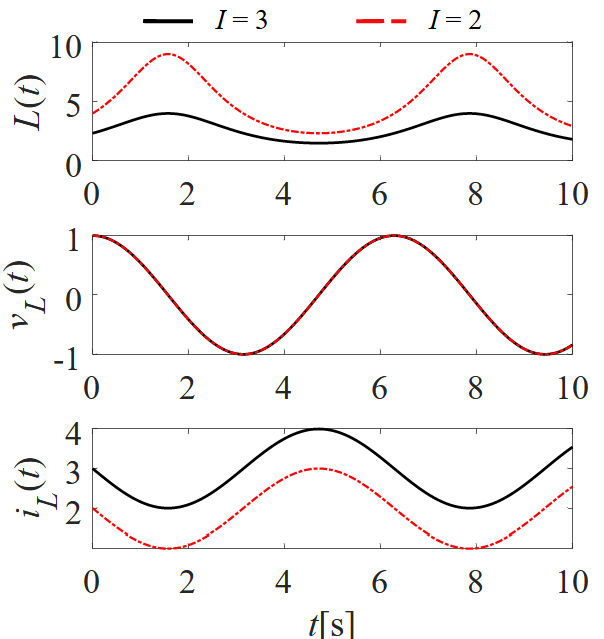
Figure 3: Stabilization of the non-Foster $L(t)C$ resonator with a positive-valued time modulated $L(t)>0$. (a) Effect of varying the equivalent inductance $L_{\mathrm{eq}}$ (for $c_{1}=10$, $I=3$ A). (b) Effect of varying the DC current source (for $c_{1}=10$, $L_{\mathrm{eq}}=-1$ H). In all cases, we have considered $C=-1$ F.

Figure 3 illustrates a numerical example involving the use of the time modulation in eq. (11) and the stabilization of the non-Foster resonator. Top, middle and bottom panels represent the applied time modulated $L(t)$, the voltage in the time-varying inductor $v_{L}(t)$, and the current in the time-varying inductor $i_{L}(t)$, respectively. Figure 3(a) shows two different scenarios for a $L(t)C$ resonator with $C=-1$ F. The selected time modulations, which follow the expression of eq. (11), are positive in both cases, but lead to very different voltage and current curves. The black curve, where the time-varying modulation of $L(t)$ mimics the action of a positive-valued time-invariant equivalent inductance, represents an unstable case. See how the voltage and current grow exponentially over time. On the other hand, the red curve represents a stable case, with $L(t)$ mimicking an equivalent negative-valued time-invariant $L_{\mathrm{eq}}$. In this case, the temporal variation is a periodic oscillation of frequency $\omega_{\mathrm{eq}}$. Figure 3(a) clearly shows how the non-Foster $L(t)C$ resonator can be stabilized with a positive modulation $L(t)>0$.

Figure 3(b) illustrates the effect of the DC current source $I$ for a fixed equivalent inductance $L_{\mathrm{eq}}=-1$ H. As seen, the DC current source has no effect on the voltage $v_{L}(t)$. This is because the capacitor blocks its DC component. Conversely, the effect of $I$ is visible in the current $i_{L}(t)$. The DC current source simply raises the current in the inductor by a value of $I$. Additionally, although not explicitly shown, the constant $c_{1}$ has no effect on either voltage or current. From a practical perspective, the constant $c_{1}$ should be considered as a free parameter that, together with the DC current, helps to create a positive modulation for all time instants.

Figure 4: Dynamic reconfiguration of frequency in the non-Foster $L(t)C$ resonator. Parameters: $C=-1$ F, $I=5$ A, $c_{1}=10$.

Playing with the value of $L_{\rm eq}$ gives a route to dynamically tune the frequency $\omega_{\mathrm{eq}}$ of the already stabilized non-Foster circuit. This represents an interesting difference with respect to the conventional time-invariant $LC$ circuits, whose natural oscillation frequency is fixed and cannot be changed for a given inductor and capacitor. Thus, the $L(t)C$ circuit can be used as a frequency reconfiguration. Figure 4 illustrates this functionality. The value of $L_{\mathrm{eq}}$ is dynamically changed three times using three different temporal modulations of the positive-valued $L(t)$: from $L_{\mathrm{eq1}}=-1$ H to $L_{\mathrm{eq2}}=-1/9$ H, and then to $L_{\mathrm{eq3}}=-1/4$ H. For a capacitor $C=-1$ F, the associated equivalent frequencies are $\omega_{\mathrm{eq1}}=1$ rad/s, $\omega_{\mathrm{eq2}}=4\omega_{\mathrm{eq1}}$, $\omega_{\mathrm{eq3}}=2\omega_{\mathrm{eq1}}$, respectively. Figure 4(a) shows the time-varying inductance $L(t)$ that creates the three equivalent inductances. Figure 4(b) illustrates how the voltage in the inductor dynamically changes as a result of changing $L(t)$. Results show that frequency reconfiguration/tuning can be achieved with the non-Foster resonator. It should be noted that the stability of the results is also dependent on the discontinuities generated in the changes of $L(t)$ and the applied initial conditions. Moreover, it is expected that frequency tuning can also be achieved with the analogue Foster version of the resonator, with positive $C$ and a time modulation of $L(t)$ that mimics positive equivalent inductances.

IV Conclusion

In this paper, inspired by Kapitza’s ideas, we have shown that non-Foster $L(t)C$ resonators with time-varying inductors and negative capacitors can be stabilized with the inclusion of temporal modulations. We have found a connection between Kapitza’s work on the inverted pendulum with a mechanically-vibrating base and time-modulated electric circuits. Eq. (8) provides a time modulation of $L(t)$ to create a one-to-one correspondence between the angle $\theta(t)$ in Kapitza’s pendulum and the current $i(t)$ in the non-Foster $L(t)C$ circuit. We have described how $i(t)$ essentially represents an amplitude-modulated version of $\theta(t)$. Unfortunately, the expression of $L(t)$ in eq. (8) involves negative values and is not convenient from a practical perspective. In order to find a $L(t)>0$ that stabilizes the non-Foster circuit with $C<0$, we apply the technique introduced in [32]. With the positive $L(t)>0$ given by eq. (11) (and the addition of a DC current source $I$), we mimic the behavior of an equivalent negative inductor $L_{\mathrm{eq}}<0$, thus stabilizing the non-Foster circuit. Moreover, how the oscillation frequency $\omega_{\mathrm{eq}}$ of the already stabilized circuit can be reconfigured in real time, giving a route for frequency tuning. These results provide a new approach for stabilizing electric circuits through time modulations and suggest Vibrational Electromagnetics as a foundation for applications in more intricate systems and complex media.

Supplementary Material

Antonio Alex-Amor, Grigorii Ptitcyn, Nader Engheta

University of Pennsylvania, Department of Electrical and Systems Engineering,
Philadelphia, Pennsylvania 19104, United States

Kapitza’s Inverted Pendulum

Equations

Let us consider the Kapitza’s inverted pendulum shown in Figure 1 [1, 2]. The center pivot is driven to oscillate up and down, according to the function $f(t)$. The position of the point mass $m$ in the Cartesian coordinate system is described by the coordinates

$$x(t)=l\sin(\theta)\,,$$ (S1)

$$y(t)=l\cos(\theta)+f(t)\,.$$ (S2)

When $f(t)=\delta\cos(\Omega t)$, the Lagrangian of this lossless system is

$$L=\frac{1}{2}m\left[l^{2}(\theta^{\prime})^{2}+2l\delta\Omega\sin(\Omega t)\sin(\theta)\,\theta^{\prime}+\delta^{2}\Omega^{2}\sin^{2}(\Omega t)\right]-mg\left[l\cos(\theta)+\delta\cos(\Omega t)\right]\,,$$ (S3)

where the first addend represents the kinetic energy, and the second addend represents the potential energy (negatively signed) of the inverted pendulum. The superscript (’) represents the first derivative with respect to time.

The application of the Euler-Lagrange equations, $d(\partial L/\partial\theta^{\prime})/dt-\partial L/\partial\theta=0$, leads to a second-order nonlinear ordinary differential equation that describes the evolution of the angle $\theta$ as a function of time:

$$\theta^{\prime\prime}(t)+\sin\left[\theta(t)\right]\left[\alpha\Omega^{2}\cos(\Omega t)-\omega_{0}^{2}\right]=0\,,$$ (S4)

with $\alpha\equiv\delta/l$ and $\omega_{0}^{2}\equiv g/l$ being a dimensionless constant and the square of the natural oscillation frequency, respectively. Note that in the case that the pendulum is not driven ($\delta=0$), the former ODE reduces to the one of the conventional simple pendulum.

Slow and Fast Components

The governing ODE for the pendulum has a difficult analytical treatment [1, 2]. Kapitza, based on the idea of having a high-frequency vibrating component of different characteristics from the natural oscillation frequency of the pendulum, decided to split the angle $\theta$ into two terms: the slow component $\theta_{s}(t)$ and the fast component $\theta_{f}(t)$. The slow component is of high amplitude and low frequency, while the fast component is of small amplitude and high frequency. Thus, the ODE can be rewritten as

$$\theta_{s}^{\prime\prime}(t)+\theta_{f}^{\prime\prime}(t)+\sin\left(\theta_{s}(t)+\theta_{f}(t)\right)\left[\alpha\Omega^{2}\cos(\Omega t)-\omega_{0}^{2}\right]=0\,.$$ (S5)

From the fast component’s perspective, the slow component is practically constant over the fast period $T=2\pi/\Omega$. Additionally, $|\theta_{f}(t)|\ll|\theta_{s}(t)|$. Under this assumptions, eq. (S5) reduces to the following equation for the ODE of the fast component:

$$\theta_{f}^{\prime\prime}(t)+\alpha\Omega^{2}\cos(\Omega t)\sin(\theta_{s})\approx 0\,$$ (S6)

whose solution will be of the form

$$\theta_{f}(t)\approx\alpha\cos(\Omega t)\sin(\theta_{s})\,.$$ (S7)

As this equation shows, the fast component is a sort of small-amplitude version of the fast component ($\theta_{f}\propto\alpha\sin(\theta_{s})$) that vibrates very fast at a frequency $\Omega$.

In order to extract the ODE for the slow component, eq. (S5) can be time-averaged over the fast period $T=2\pi/\Omega$ with the information about $\theta_{f}(t)$ that it has been already extracted. This leads to

$$\theta_{s}^{\prime\prime}(t)+\sin\left(\theta_{s}(t)\right)\left[\frac{\alpha^{2}\Omega^{2}}{2}\cos(\theta_{s}(t))-\omega_{0}^{2}\right]\approx 0\,.$$ (S8)

Eq. (S8) gives us information about the temporal evolution of the slow component $\theta_{s}$. With information about the slow and fast components, the whole solution, $\theta(t)=\theta_{s}(t)+\theta_{f}(t)$, can be reconstructed. Although eq. (S8) cannot be easily treated analytically, it can be further manipulated in order to work directly with potentials and thus derive information about the stable positions, $\theta=\{0,\pi\}$, in the inverted pendulum.

Inclusion of Losses: Non-Foster $RL(t)C$ Circuit

Let us consider a non-Foster $RL(t)C$ resonator formed by a time-invariant capacitor of negative capacitance $C<0$, a time-invariant resistor $R$ and a time-varying inductor with positive-valued inductance $L(t)>0,\forall t$. Circuit elements $R$, $L(t)$, and $C$ are connected in series. Voltage-current relations in the capacitor, resistor and inductor are given by $i_{C}(t)=C\,dv_{C}(t)/dt$, $v_{R}(t)=Ri_{R}(t)$ and $v_{L}(t)=d[L(t)\,i_{L}(t)]/dt$, respectively. Considering that $i_{C}(t)=i_{R}(t)=i_{L}(t)=i(t)$ and $v_{C}(t)+v_{R}(t)+v_{L}(t)=0$, circuit analysis leads to the ODE defined in eq. (1), but now with variable coefficients

$$p(t)=\frac{2L^{\prime}(t)+R}{L(t)},\quad q(t)=\frac{\frac{1}{C}+L^{\prime\prime}(t)}{L(t)}\,.$$ (S9)

The inclusion of the resistor $R$ incorporates a new addend, $i^{\prime}(t)R/L(t)$, to the governing ODE. This new addend is essentially in charge of incorporating losses to the system and attenuating the current $i(t)$ over time if $R>0$.

Stability Theorem for $\phi(t)$

Theorem 8.5 in [46] gives guidance on the stability of one system based on the known stability of another. The mentioned theorem states that the solutions of linear time-varying system of the form

$$\mathbf{\Phi}^{\prime}(t)+\big{[}X_{0}+\Delta\mathbf{X}(t)\big{]}\mathbf{\Phi}(t)=\mathbf{0}$$ (S10)

are stable provided that the solutions of

$$\mathbf{\Phi}^{\prime}(t)+X_{0}\mathbf{\Phi}(t)=\mathbf{0}$$ (S11)

are stable too and that $\int_{0}^{\infty}||\Delta\mathbf{X}(t)||\,dt<\infty$, where $X_{0}$ is a constant.

The stability of eq. (5),

$$\phi^{\prime\prime}(t)+\frac{1}{L(t)C}\,\phi(t)=0\,,$$

and, thus, of the whole non-Foster circuit, for a modulation of the form $L(t)=L_{\mathrm{eq}}+c_{1}/i(t)$ can be proven with the application of Theorem 8.5. This is because the modulation $L(t)$, which is formed by the addition of a constant $L_{\mathrm{eq}}$ and a time-varying term $c_{1}/i(t)$, resembles the form $X_{0}+\Delta\mathbf{X}(t)$.

We know that the solutions of

$$\phi^{\prime\prime}(t)+\frac{1}{L_{\mathrm{eq}}C}\,\phi(t)=0$$ (S12)

are stable if the constant term $1/(L_{\mathrm{eq}}C)$ is positive. For the case considered in the manuscript, $C<0$ and $L_{\mathrm{eq}}<0$, the term $1/(L_{\mathrm{eq}}C)>0$, thus the solutions $\phi(t)$ in eq. (S12) are stable. Therefore, the application of Theorem 8.5 in [46] states that the solutions of eq. (5) are stable too, so does the non-Foster circuit, if the applied modulation is of the form $L(t)=L_{\mathrm{eq}}+c_{1}/i(t)$, with $L_{\mathrm{eq}}<0$ and $C<0$. This holds as long as the time-varying term $c_{1}/i(t)$ does not lead to a divergent improper integral ($\int_{0}^{\infty}||\Delta\mathbf{X}(t)||\,dt<\infty$). i.e., as long as $i(t)\neq 0\,\forall t$ and $i(t)$ is bounded and decaying over time. Currents $i(t)$ of the form $i(t)=[I+i_{0}\sin(\omega t)]\mathrm{e}^{-at}\neq 0$ fulfill this condition. This selection of $i(t)$ is essentially similar to the one chosen in the manuscript [see eq. (11)], since it is possible to select an attenuation factor $a$ small enough ($a\rightarrow 0^{+}$) so that the decay is not appreciable over time and the non-Foster system is stable.

List of Media and Included Animations

The following animations regarding Kapitza’s inverted pendulum are included as part of the supplementary material:

• “KapitzasPendulum_Omega141omega0.mp4”. Parameters: $\delta=0.1$, $l=1$ m, $\Omega=14.1\omega_{0}$.

• “KapitzasPendulum_Omega15omega0.mp4”. Parameters: $\delta=0.1$, $l=1$ m, $\Omega=15\omega_{0}$.

• “KapitzasPendulum_Omega20omega0.mp4”. Parameters: $\delta=0.1$, $l=1$ m, $\Omega=20\omega_{0}$.

In all cases, initial conditions are $\theta(0)=20$ deg, $\theta^{\prime}(0)=0$. In order of appearance, the first animation ($\Omega=14.1\omega_{0}$) shows an unstable solution, while the second ($\Omega=15\omega_{0}$) and third ($\Omega=20\omega_{0}$) animations show stable solutions. The modulation frequency $\Omega$ in the first animation is pretty close to the limit frequency $\Omega_{\mathrm{lim}}$ that marks stability. The vibrating base almost counter the effect of gravity, but the modulation frequency is not high enough and the pendulum eventually falls. Second and third animations illustrate how the mechanical vibration counters the effect of gravity and keeps the pendulum swinging periodically. See how the slow frequency increases (the period decreases) as the modulation frequency $\Omega$ increases too.