Applying Astronomical Solutions and Milanković Forcing in the Earth Sciences

Abstract

Astronomical solutions provide calculated orbital and rotational parameters of solar system bodies based on the dynamics and physics of the solar system. Application of astronomical solutions in the Earth sciences has revolutionized our understanding in at least two areas of active research. ($i$) The Astronomical (or Milanković) forcing of climate on time scales $\stackrel{{\scriptstyle>}}{{\sim}}\$10 kyr and ($ii$) the dating of geologic archives. The latter has permitted the development of the astronomical time scale, widely used today to reconstruct highly accurate geological dates and chronologies. The tasks of computing vs. applying astronomical solutions are usually performed by investigators from different backgrounds, which has led to confusion and recent inaccurate results on the side of the applications. Here we review astronomical solutions and Milanković forcing in the Earth sciences, primarily aiming at clarifying the astronomical basis, applicability, and limitations of the solutions. We provide a summary of current up-to-date and outdated astronomical solutions and their valid time span. We discuss the fundamental limits imposed by dynamical solar system chaos on astronomical calculations and geological/astrochronological applications. We illustrate basic features of chaotic behavior using a simple mechanical system, i.e., the driven pendulum. Regarding so-called astronomical “metronomes”, we point out that the current evidence does not support the notion of generally stable and prominent metronomes for universal use in astrochronology and cyclostratigraphy. We also describe amplitude and frequency modulation of astronomical forcing signals and the relation to their expression in cyclostratigraphic sequences. Furthermore, the various quantities and terminology associated with Earth’s axial precession are discussed in detail. Finally, we provide some suggestions regarding practical considerations.

1 Introduction

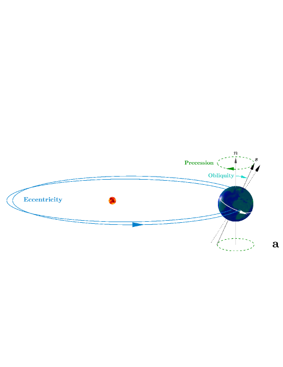
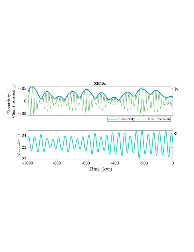
Figure 1: Example of orbital parameters and their values frequently used in the Earth sciences. (a) Illustration of orbital eccentricity (recent main periods $\sim$100 and 405 kyr), precession ($\sim$20 kyr), and obliquity ($\sim$41 kyr), often called Milanković cycles (for geometrical illustrations of their physical meaning, see also Figs. 2 and 14). For illustration, Earth’s orbital eccentricity is highly exaggerated. For an elliptical orbit, the sun is located at one of the ellipses’ foci. Obliquity is the angle between Earth’s spin axis (spin vector $s$) and the orbit normal (unit vector $n$ perpendicular to Earth’s orbital plane = ecliptic, see Table 1). Viewed from ecliptic north, Earth’s rotation (spin) is counterclockwise (from west-to-east, or eastward). Earth’s orbital motion is in the same direction (prograde). Axial precession (precession of the equinoxes) is in the opposite direction (retrograde, green arrow). Orbital parameter values shown here are from/based on the orbital solution ZB18a (Zeebe and Lourens, 2019, 2022a) over the past 1 Myr. (b) Earth’s orbital eccentricity (blue) from ZB18a and climatic precession (green) based on ZB18a. (c) Obliquity of Earth’s spin axis based on ZB18a.

The term “astronomical solution” ($\cal AS$) as used here refers to calculated planetary orbital and rotational parameters over time based on known solar system physics at a specified point in time. Mathematically, an $\cal AS$ for the planetary orbits represents a solution to the equations of motion of the solar system with initial conditions at time $t_{0}$ for the positions, velocities, and masses of the solar system bodies included in the calculation. Here we will focus specifically on $\cal AS$s that have direct applications in the Earth sciences, for instance, in geology, paleoclimatology, astrochronology, and cyclostratigraphy; i.e., $\cal AS$s that provide accurate values for Earth’s orbital parameters in the past (for a specific example, see Fig. 1). Thus, while a general review of $\cal AS$s may start historically with the work of Johannes Kepler, we start with the work of Milutin Milanković, a Serbian engineer and mathematician (1879-1958).

Although not the first to propose astronomically-driven climate change on Earth (for a review, see Emiliani, 1995), Milanković worked out an astronomical theory to calculate the effects of secular (‘slow’) changes in insolation on Earth’s climate and was primarily interested in applying the astronomical theory to the ice age problem. In 1941, Milanković summarized his findings spanning thirty years of work in a 633-page volume to the Serbian Royal Academy (Milanković, 1941). Milanković used an $\cal AS$ that included elements of Leverrier’s work and contributions from Mišković (see Milanković, 1941, p. 335 ff.). Notably, Milanković’s astronomical theory of paleoclimate was far from accepted at the time and was virtually ignored for decades before being recognized by a larger community that realized its merit (e.g., Emiliani, 1955; Broecker, 1966; Imbrie and Kipp, 1971; Hays et al., 1976; Berger, 1978). Today, there is overwhelming evidence that Earth’s climate is paced by astronomical cycles on time scales $\stackrel{{\scriptstyle>}}{{\sim}}\$10 kyr. Based on work from the late 1800s, a new $\cal AS$ was calculated by Brouwer and van Woerkom (1950) and subsequently applied to test the astronomical theory of climate change (e.g., van Woerkom, 1953; Broecker, 1966). Importantly, the $\cal AS$s up to that point were based on so-called low-order perturbation theory, sometimes dubbed secular analytic theory, or Laplace-Lagrange solution (for details and history, see Murray and Dermott, 1999; Ito and Tanikawa, 2007), which only allows for quasi-periodic, i.e., non-chaotic, solutions. A simple example of a quasi-periodic function is the sum of two periodic functions (single frequency each) with an irrational frequency ratio.

Table 1: Notation and values employed in this paper (frequently used variables).

Symbol	Meaning	Value I/A	Unit	Note
$a$	Semimajor axis		au	Element 1
$e$	Orbital eccentricity		–	Element 2
$I$	Orbital inclination		deg	Element 3
$\Omega$	Orbit LAN  a		rad	Element 4
$\omega$	Orbit AP  b		rad	Element 5
$\nu$	True anomaly		rad	Element 6
$\varpi$	Orbit LP  c		rad	see text
$N$	Total No. of bodies  d		–
$\Sun,\ \Earth,\ \Moon$	Sun, Earth, Moon/Lunar		–	or subscript S,E,L
$M_{\Sun}$	Central mass		1.0 or kg
$m_{i}$	Mass of body $i$		$M_{\Sun}$ or kg
$n_{i}$	Mean motion		rad d-1
$\epsilon$	Obliquity angle		deg
$\epsilon$0	Obliquity Earth $t_{0}$	23.4392911	deg	Fränz and Harper (2002)
$\phi$	Precession angle  e
$\Psi_{0}$	Luni-solar prec. rate $t_{0}$ f	$50.3848$	′′ y-1	Capitaine et al. (2003)
$\Psi_{A}$	Accumulated angle		′′	$\dot{\Psi}_{A}=\Psi$
$p_{A}$	General prec. in long.g		′′	$p_{A}=-\mbox{$\phi$}$
$\bar{\omega}$	Orbit LPX h			$\mbox{$\bar{\omega}$}=\mbox{$\varpi$}+|\mbox{$\phi$}|$  e
$\bar{p}$	Climatic precession			$\mbox{$\bar{p}$}=e\sin\mbox{$\bar{\omega}$}$
$s$	Spin vector
$n$	Orbit normal
$H$	Dynamical ellipticity	$\sim$0.00328	–
$k^{2}$	(Gauss grav. const.)2	$0.01720209895^{2}$	see i
au	Astronomical unit	$1.495978707\mbox{$\times 10^{11}$}$	m
$G\mbox{$M_{\Sun}$}$	Sun GP j	$1.32712440041\mbox{$\times 10^{20}$}$	$\rm m^{3}~{}s^{-2}$
$\mbox{$M_{\Sun}$}/(\mbox{$m_{\Earth}$}+\mbox{$m_{\Moon}$})$	Mass ratio	$328900.5596$	–
$\mbox{$m_{\Earth}$}/\mbox{$m_{\Moon}$}$	Mass ratio	$81.300568$	–
$\Omega_{E}$	Earth’s angular speed	$7.292115\mbox{$\times 10^{-5}$}$	rad s-1	at $t_{0}$

^a LAN = Longitude of Ascending Node. ^b AP = Argument of Perihelion. ^c LP = Longitude of Perihelion. ^d Including the central mass. ^e Axial precession is retrograde (Section 3.1, Fig. 14), hence $\dot{\mbox{$\phi$}}_{0}$ is taken negative here (time derivatives are denoted by “dot”, $\dot{\mbox{$\phi$}}=d\phi/dt$). ^f Conventionally, $\Psi$ is taken positive (Section 3.1). ^g General precession in longitude. ^h LPX = LP from the moving equinox. $\bar{\omega}$ (“omega bar”) is not be confused with $\varpi$ (“varpi”). Various symbols are used for $\bar{\omega}$ in the literature. ⁱ General unit of $k$: $\rm au^{3/2}~{}d\mbox{${}^{-1}$}~{}M^{-1/2}_{0}$, dimensionless in astronomical units, also rad d^-1 when e.g., equated with $n_{i}$. ^j GP = Gravitational Parameter.

From a practical perspective, the next significant step in $\cal AS$ development followed in the 1970s and provided Earth’s orbital parameters over the past few million years at improved accuracy (Bretagnon, 1974; Berger, 1976, 1977). The $\cal AS$s were still based on secular perturbation theory but included higher-order terms in series expansions with respect to eccentricity, inclination, and planetary masses (Bretagnon, 1974; Duriez, 1977; Laskar, 1985). Taking advantage of the accelerating computer power in the 1980s, Sussman and Wisdom (1988) studied the outer planets using full numerical integrations over 845 Myr on the Digital Orrery and showed that the motion of Pluto is chaotic. (The Digital Orrery was a special-purpose computer built specifically for studying planetary motion (Applegate et al., 1985), named after orrery, a mechanical model of the solar system that illustrates the relative positions and motions of the planets and moons.) Higher-order, averaged equations of the secular evolution of the inner and outer planets also showed chaos, with a “Lyapunov time” for the inner solar system of only $\sim$5 Myr (Laskar, 1989). The Lyapunov time is a metric to characterize chaos in dynamical systems and represents the time scale of exponential divergence (e-folding time) of nearby trajectories (see, e.g., Murray and Dermott, 1999).

The first fully numerical and “direct” long-term integration (the past 3 Myr) of the eight planets and Pluto directly based on the equations of motion (not analytical) was carried out by Quinn et al. (1991) using a multistep method. Quinn et al. (1991) showed that the model and secular theory predictions of, e.g., Earth’s orbital eccentricity and obliquity by Berger (1978), were inaccurate beyond about 1-1.5 Myr in the past, although subsequent updates by Berger and Loutre (1992) showed better agreement with Quinn et al. (1991). Notably, the $\cal AS$s based on earlier physics models and low/intermediate-order analytic secular perturbation theory were (a) by design unable to reveal the chaotic behavior of the the solar system and (b) were only accurate over the past few Myr. These results suggested that either fully numerical approaches or very high-order secular solutions were required for accurate applications in the Earth sciences. Laskar (1990) provided a long-term orbital solution that was obtained using an extended, averaged secular system. Regarding long-term solar system integrations, we note that Ito and Tanikawa (2002) performed full numerical, long-term integrations of up to 5 Gyr of the eight planets and Pluto. However, the study’s focus was long-term stability, rather than accuracy for geological applications and omitted several second-order effects (i.e., general relativity, a separate Moon, and asteroids). In 2003, Varadi and co-workers published the results of a direct, fully numerical integration of the eight planets over the past 100 Myr using a Störmer multistep scheme, which revealed large differences to the results of Laskar (1990) already around $-24$ Myr (Varadi et al., 2003) (past time in $\cal AS$s is negative here, see footnote 1). The early 2000s effectively marked the end of $\cal AS$ based on secular perturbation theory for any serious geological application. Subsequent $\cal AS$ employed in, for instance, astrochronology and cyclostratigraphy are based on full numerical integrations (Laskar et al., 2004, 2011; Zeebe, 2017; Zeebe and Lourens, 2019, 2022a, 2022b; Zeebe and Lantink, 2024a, b). The most recent numerical solutions are described in more detail in Section 2.5.

Over the past few decades, the improvement in accuracy of $\cal AS$s has permitted the development of the astronomical time scale (ATS, see Table 2), which has transformed the dating of geologic archives. Simply put, the ATS represents an accurate astronomical calendar used in the Earth sciences based on the motion of solar system bodies to study and explain Earth’s geologic history (for further reading, see, e.g., Montenari, 2018). In addition to accurate relative (floating) age models and chronologies (see also Section 3.5), astrochronology provides highly accurate geological dates with small error margins. For example, recent efforts have dated the Paleocene-Eocene Thermal Maximum (PETM) onset at $56.01\pm 0.05$ Ma and the Cretaceous-Tertiary Boundary at $65.96$ to $65.52$ Ma (Zeebe and Lourens, 2019, 2022b). “Tertiary” is used informally here, not as a formal division (ICS, 2005). Astrochronology has made formidable progress in geological dating through deep-sea drilling and age-model tuning to $\cal AS$s, which led to the calibration of critical intervals of the geologic time scale, particularly in the early and mid-Cenozoic (e.g., Hinnov, 2000; Zachos et al., 2001; Lourens et al., 2005; Westerhold et al., 2008; Hilgen et al., 2010, 2015; Liebrand et al., 2016; Meyers and Malinverno, 2018; Lauretano et al., 2018; Li et al., 2018; Hinnov, 2018; Zeebe and Lourens, 2019; Westerhold et al., 2020; Zeebe and Lourens, 2022a, b).

Importantly, an increasing number of studies at the current frontier of cyclostratigraphic research are pushing the boundaries into deep time, thereby providing unique insight into astronomical forcing of paleoclimate and solar-system evolution over hundreds of millions to billions of years (e.g., Zhang et al., 2015; Ma et al., 2017; Meyers and Malinverno, 2018; Kent et al., 2018; Lantink et al., 2019; Olsen et al., 2019; Sørensen et al., 2020; Lantink et al., 2022, 2023, 2024; Zeebe and Lantink, 2024a, b; Malinverno and Meyers, 2024; Wu et al., 2024). A critical ongoing task is to use the geological record to confirm and map the solar system’s chaotic behavior, reconstruct the Earth-Moon history, and develop a “Geological Orrery”, in analogy to the mechanical and Digital Orrery (see above and Olsen et al., 2019). For more information on astronomical forcing and astronomical solutions in deep time, see Section 3.5.

Table 2: Frequently used acronyms

Acronym	Meaning
$\cal AS$	Astronomical Solution
AM	Amplitude Modulation
ATS	Astronomical Time Scale
EC	Eccentricity Cycle
ETP	Eccentricity, Tilt, Precession
FM	Frequency Modulation
FFT	Fast Fourier Transform
LEC	Long Eccentricity Cycle
OS	Orbital Solution
PT	Precession-Tilt
SEC	Short Eccentricity Cycle
VLEC	Very Long Eccentricity Cycle
VLN	Very Long eccentricity Node

Today, $\cal AS$s and the ATS represent the backbone of astrochronology and cyclostratigraphy, and are widely used in the Earth sciences, including areas of geology, geophysics, paleoclimatology, paleontology, and more. The applications are broad, ranging from high-fidelity dating (establishing highly accurate geological ages and chronologies) and reconstructing forcing/insolation patterns and their effects on paleoclimate — to the evolution of the Earth-Moon system and nonlinear dynamics (to name just a few, for recent summaries, see Montenari, 2018; Hinnov, 2018; Cvijanovic et al., 2020; Lourens, 2021; De Vleeschouwer et al., 2024; Wu et al., 2024).

1.1 The Main Milanković Cycles

The focus of this review is on astronomical solutions and forcing, rather than on the forcing’s effects on Earth’s climate through insolation changes. Nevertheless, the main Milanković cycles are very briefly summarized here (for details and reviews, see, e.g., Milanković, 1941; Hays et al., 1976; Broecker, 1985; Berger and Loutre, 1994; Muller and MacDonald, 2002; Hinnov, 2018; Lourens, 2021). As mentioned above, the main Milanković cycles usually refer to precession, obliquity, and eccentricity (for illustration and main periods, see Fig. 1). To be precise, we refer here to climatic precession (see Section 3.1). Climatic precession and obliquity affect the geographical distribution of insolation over time, whereas eccentricity affects the total insolation Earth receives (precession and obliquity do not). For instance, climatic precession shifts the positions of the equinoxes relative to Earth’s eccentric orbit (see Figs. 1 and 14). Hence, if at a given time northern hemisphere summer occurs at perihelion, it will occur at aphelion about 10 kyr later (perihelion and aphelion refer to the closest and farthest distance from the Sun along Earth’s orbit, see Fig. 2). As a result, the insolation at a given calendar day and latitude on Earth varies with climatic precession over time (one critical element in the pacemaking of the ice ages, e.g., Hays et al., 1976). The effects of climatic precession are anti-phased between the hemispheres.

Obliquity changes the solar incidence angle of insolation at a given latitude on Earth (see Figs. 1 and 14). Obliquity thus affects the seasonal contrast of insolation (in-phase between the hemispheres and increasingly pronounced toward higher latitudes). For instance, at an obliquity angle $\mbox{$\epsilon$}=0\mbox{${}^{\circ}$}$, the tilt-induced seasons would disappear, whereas at $\mbox{$\epsilon$}=90\mbox{${}^{\circ}$}$, the tilt-induced seasons would be extreme (as is the case on Uranus with an obliquity of $\sim$98^∘). Earth’s recent obliquity varies between minima and maxima of about $22.0\mbox{${}^{\circ}$}$ and $24.5\mbox{${}^{\circ}$}$ over a 41-kyr main period (Fig. 1), which causes substantial changes in Earth’s climate — often enhanced when continental ice sheets are present (for summaries, see, e.g., Lourens, 2021; De Vleeschouwer et al., 2024). Local insolation changes due to obliquity (and climatic precession) may be sizable. For example, at $65\mbox{${}^{\circ}$}$N (Jun 21) insolation varies up to $\sim$120 W m^-2 over the past 1 Myr.

Earth’s orbital eccentricity ($e_{\Earth}$) impacts insolation in multiple ways. For example, on precessional time scales, $e_{\Earth}$ modulates the amplitude of precession, which, in turn, affects insolation (Fig. 1). On annual time scales, $e_{\Earth}$ influences the total insolation Earth receives along its orbit, as the distance ($r$) to the Sun varies (see Fig. 1 and 2, for $\mbox{$e_{\Earth}$}\neq 0$). At perihelion and aphelion $r$ is equal to $a(1-\mbox{$e_{\Earth}$})$ and $a(1+\mbox{$e_{\Earth}$})$, respectively, where $a$ is the semimajor axis (e.g., Danby, 1988). Given that the insolation with respect to Earth’s cross section at distance $r$ is proportional to $r^{-2}$, the insolation ratio at perihelion vs. aphelion is:

$$(1+\mbox{$e_{\Earth}$})^{2}/(1-\mbox{$e_{\Earth}$})^{2}\ ,$$ (1)

which yields $\sim$7% and 27% at present $\mbox{$e_{\Earth}$}=0.0167$ and $\max\{\mbox{$e_{\Earth}$}\}\simeq 0.06$, respectively (see Fig. 1). As a result, eccentricity also induces “seasons”, which are, however, hemispherically symmetric and presently smaller than the tilt-induced seasons. The total mean annual insolation (or energy $W$) Earth receives is proportional to (e.g., Berger and Loutre, 1994):

$$W\propto\left(1-\mbox{$e_{\Earth}$}^{2}\right)^{-\frac{1}{2}}\ .$$ (2)

The absolute effect of the factor $\left(1-\mbox{$e_{\Earth}$}^{2}\right)^{-\frac{1}{2}}$ at present is small ($\sim$0.014%), compared to a circular orbit with $\mbox{$e_{\Earth}$}=0$. However, for long-term variations, the ratio of $W$ at different $e_{\Earth}$’s matters. For example, between the present $\mbox{$e_{\Earth}$}=0.0167$ and $\mbox{$e_{\Earth}$}=0.06$, $W$ increases by $\sim$0.17%, which is not negligible because it raises the total, global energy received. At a solar constant of 1370 W m^-2, 0.17% amounts to 2.3 W m^-2 (0.6 W m^-2 when distributed over Earth’s surface, i.e., reduced by factor 4). For comparison, a doubling of CO₂ in Earth’s atmosphere is equivalent to $\sim$3.7 W m^-2 of radiative forcing. Thus, orbital eccentricity forcing (in W m^-2) may appear small compared to local changes from climatic precession and obliquity (see above). However, the difference is that eccentricity forcing is global. Finally, and regardless of whether precession, obliquity, or eccentricity forcing is involved, caution is advised when attempting to predict the impact of astronomical forcing on Earth’s climate, because the climate system response is highly non-linear.

Regarding the stratigraphic recording of the climate system response (say, in sedimentary sequences), it is noteworthy that the response of the sedimentary system to climate perturbations is also inherently non-linear. Thus, the translation of astronomical cycles to sedimentary cycles is modified by two non-linear transfer functions.

1.2 Types of Astronomical Solutions

Two types of astronomical solutions are discussed in the following: orbital solutions (OSs) and precession-tilt (PT) solutions. OSs describe the orbital dynamics of the solar system, usually considering the solar system bodies as mass points (as is the case here). OSs provide values for the orbital elements of solar system bodies over time, including orbital eccentricity and inclination (see Fig. 2). PT solutions describe the rotational dynamics of individual solar system bodies (here of the Earth), considering the physical dimensions and shape of the body. PT solutions provide values for precession and obliquity over time, e.g., based on spin axis dynamics (see Fig. 14). OS dynamics have important effects on (and are a prerequisite for) PT solutions, while the effect of rotational dynamics on OSs is generally minor (e.g., Earth-Moon dynamics, see Zeebe and Lantink, 2024b). For example, amplitude variations in Earth’s orbital inclination (due to OS dynamics) are reflected in obliquity — most evidently during intervals of reduced amplitude variation (see Zeebe, 2022). Similarly, amplitude variations in eccentricity (due to OS dynamics) are reflected in climatic precession.

1.3 Organization of Content

The remainder of this review is organized into three sections focusing on orbital solutions, precession-tilt solutions, and practical considerations (Sections 2, 3, and 4). Section 2 introduces several basic concepts for describing and analyzing orbital solutions, including orbital elements and the fundamental frequencies of the solar system. Solar system chaos is key and indispensable to understanding a variety of topics, including the limitations imposed on orbital solutions by chaotic dynamics. Chaos is therefore discussed in some detail under orbital solutions (Section 2.3). Chaos also causes critical changes in the amplitude modulation (AM) of orbital forcing signals, which, if expressed in cyclostratigraphic sequences, can be used to reconstruct the solar system’s chaotic history. Section 2.3 on solar system chaos thus precedes Section 2.4 on amplitude and frequency modulation. Furthermore, AM originates from combination terms related to the fundamental frequencies but can also be studied using eccentricity and obliquity analysis. Thus, AM is examined in some depth in two sections (2.1.4 and 2.4.1). Up-to-date orbital solutions, their valid time span (another consequence of solar system chaos), and the confusion surrounding the subject are described in Section 2.5. Importantly, the probability that a particular OS represents the actual, unique history of the solar system is near zero significantly beyond the OS’s valid time span (the details and implications are explained in Sections 2.5 and 4). Section 3 dives into the details of precession-tilt solutions, explaining the various quantities associated with Earth’s axial precession and aiming at clarifying the terminology and notation used in the literature. Up-to-date precession-tilt solutions are described in Section 3.4, as well as recently employed tools that produce inaccurate results. Another critical application of astronomical solutions beyond the direct use for astronomical tuning (e.g., absolute Cenozoic ages and chronologies) is astronomical forcing and astrochronology in deep time (see Section 3.5). Section 4 provides several recommendations for the user seeking guidance and lists selected resources for practical consideration. We close with a brief summary and outlook (Section 5).

2 Orbital Solutions

2.1 Fundamentals

2.1.1 Orbital Elements

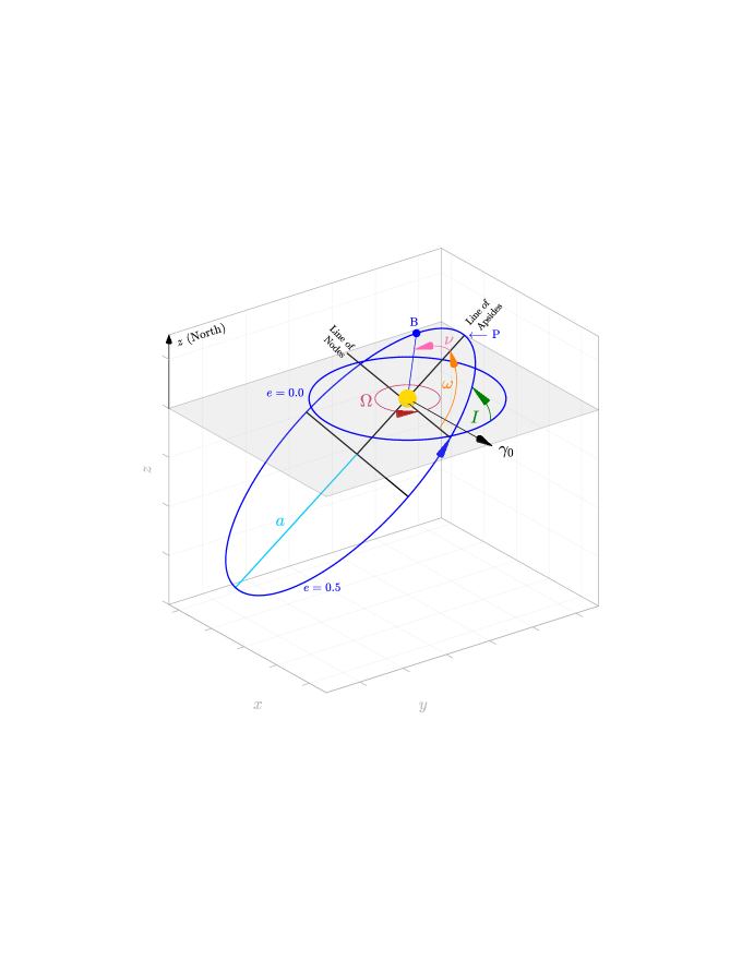
Figure 2: Illustration of elements characterizing a Keplerian orbit. $a=$ semimajor axis, $e=$ eccentricity, $I=$ inclination. $I$ is the angle measured from the fixed reference plane (gray) to the instantaneous orbit plane. Two orbits (blue, different $a$’s) are shown; the circular orbit ($e=0$, $I=0$) lies in the reference plane; the elliptic orbit ($e=0.5$) is inclined relative to the reference plane. $\mbox{$\Omega$}=$ longitude of the ascending node is measured in the reference plane from the reference point $\mbox{$\gamma$}_{0}$ to the line of nodes where the orbiting body (B) ascends, i.e., passes from south to north ($z<0$ to $z>0$, see blue arrow) through the reference plane. Hence $\Omega$ (if defined) is measured in a plane different from B’s orbital plane. In the solar system, $\mbox{$\gamma$}_{0}$ may refer to the vernal point at a fixed date. $\mbox{$\omega$}=$ argument of perihelion is measured from the ascending node to the perihelion (P). The line of apsides passes through the perihelion (P) and aphelion of the orbit (closest and farthest distance from the central body). $\nu=$ true anomaly is measured from the perihelion to the orbiting body (B).

For the reader unfamiliar with orbital parameters commonly used in astronomy, we first introduce the Keplerian elements and the notation used throughout this paper (see Fig. 2 and Table 1). Keplerian orbits include circular ($e=0$), elliptic ($0<e<1$, $a>0$), parabolic ($e=1$), and hyperbolic ($e>1$, $a<0$) orbits. To describe the orbit, six independent elements are used, five of which (for instance, $a,e,I,\mbox{$\Omega$}$, and $\omega$) define the shape and orientation of the orbit in space (for illustration, see Fig. 2). The final element (such as the true anomaly $\nu$) identifies the body’s position in the orbit and hence represents the instantaneous (rapidly changing) orbital element. Notably, the Keplerian elements are used to describe orbits in general, not only exact solutions to Kepler’s two-body problem, which can be solved analytically. In the two-body problem ($N=2$), $\nu$ varies over time, while the five elements defining orbit shape and orientation are constant, which is not the case in general ($N>2$). For example, the motion of solar system bodies such as the planets include the full planet-planet interactions and hence do not evolve on simple Kepler ellipses. Nevertheless, at a given instant in time, the orbit can be defined by Keplerian (also called osculating) elements, which refer to the orbit the body would have without perturbations (in mathematics osculate means to touch so as to have a common tangent). In the general case, the orbit’s shape and orientation change over time. The six orbital elements can be converted into the body’s Cartesian position and velocity vectors $x$ and $v$ (and vice versa) via a coordinate transformation (six degrees of freedom). Thus, the output of orbital solutions may be provided in orbital elements or Cartesian vectors, or both.

Note that for $I=0$, the line of nodes and hence $\Omega$ and $\omega$ are undefined. Nevertheless, as long as $e\neq 0$, the longitude of perihelion, $\varpi$, may always be defined (see Section 2.3 in Bate et al., 1971). $\varpi$ is measured from the reference point to the perihelion eastward (to the ascending node, if it exists, and then in the orbital plane to the perihelion). If both $\Omega$ and $\omega$ are defined, then

$$\mbox{$\varpi$}=\mbox{$\Omega$}+\mbox{$\omega$}\ .$$ (3)

In general, $\varpi$ is therefore a “dogleg” angle, as $\Omega$ and $\omega$ lie in different planes. However, this does not impede its use and utility as an orbital element. Importantly, $\varpi$ is well defined for all inclinations.

2.1.2 Eccentricity and Inclination

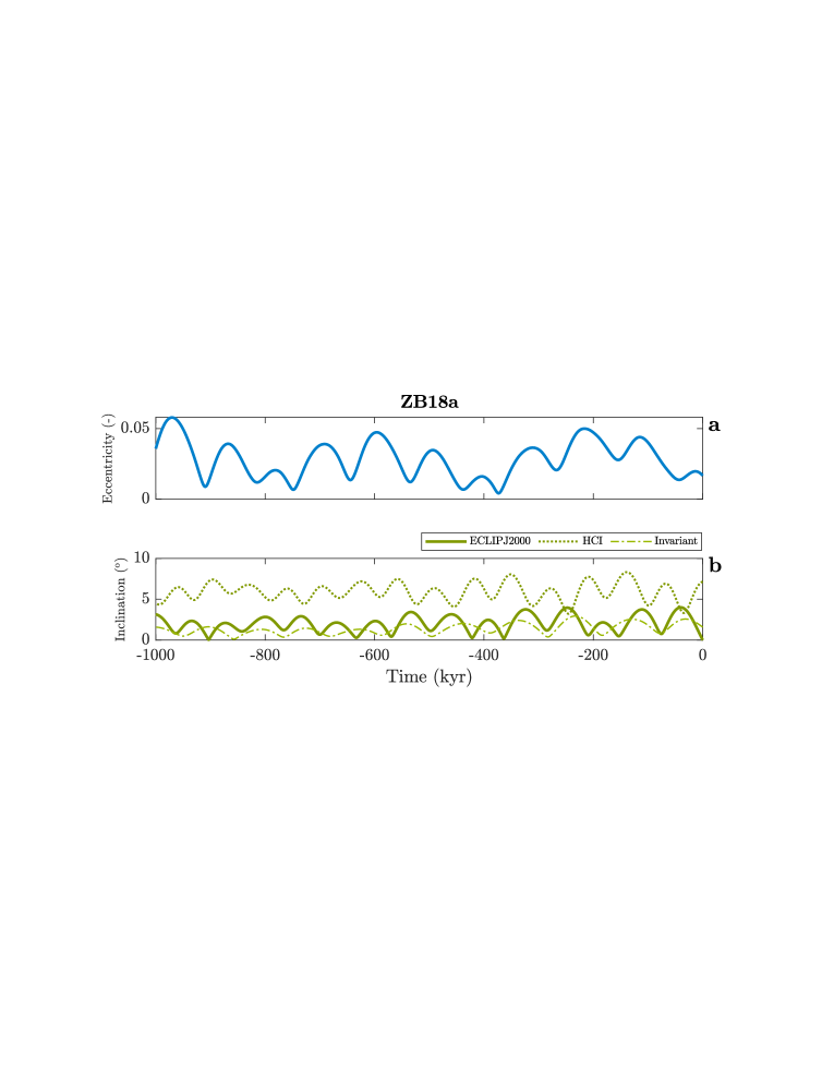
Figure 3: Earth’s orbital eccentricity and inclination from $\cal AS$ ZB18a (Zeebe and Lourens, 2019) over the past 1 Myr. For geometrical illustrations of the physical meaning of orbital eccentricity and inclination, see Figs. 2, 4, and 14. (a) Earth’s orbital eccentricity (which is independent of the reference frame). (b) Earth’s orbital inclination in different reference frames. Solid line: Ecliptic frame (ECLIPJ2000), dashed line: Heliocentric Inertial (HCI) frame (for details, see Fränz and Harper, 2002; Zeebe, 2017), dot-dashed line: invariant frame (see text).

Earth’s orbital eccentricity is among the most frequently used orbital parameters in Earth-science applications (see Fig. 3 for an example over the past 1 Myr). Cyclostratigraphic sequences, for instance, often show strong cyclicity at eccentricity frequencies (main periods of $\sim$100 kyr and 405 kyr in the recent past). Eccentricity affects the total insolation Earth receives over one year (e.g., Berger and Loutre, 1994), which in turn affects Earth’s climate (Section 1.1). Moreover, if clear axial precession signals are present in the geologic sequence, the observed precession amplitude is modulated by eccentricity (in a very simple manner, i.e., eccentricity is the envelope of climatic precession, see Fig. 1). Eccentricity is related to the shape of the orbit (not the orientation in space, see Fig. 2) and is hence independent of the reference frame used to describe the orbit. In contrast, orbital inclination depends on the reference frame, as the choice of the reference plane is arbitrary (Fig. 2). Thus, the representation of inclination may differ fundamentally between different reference frames (for a frequently used frame such as the ecliptic, see Fig. 3). However, other frames such as the invariant frame (based on the invariable plane, perpendicular to the solar system’s total angular momentum vector that passes through its barycentre) or the Heliocentric Inertial (HCI) frame (based on the orientation of the solar equator at a fixed point in time) are equally valid and are useful for e.g., accounting for effects of the solar quadrupole moment on the dynamics (for details, see Fränz and Harper, 2002; Souami and Souchay, 2012; Zeebe, 2017). Note that accurate transformations between frames generally require detailed information about the coordinate systems and, depending on the case, parameters such as initial conditions, masses, constants used, etc. (see below and Souami and Souchay (2012)).

Because of the distinct physical nature of inclination and eccentricity (see Fig. 2), orbital forcing effects (Section 1.1) due to inclination and eccentricity are principally different (for further discussion, see, e.g., Muller and MacDonald, 2002; Zeebe, 2022; Zeebe and Lantink, 2024b). Orbital inclination represents one of the controls on the obliquity of Earth’s spin axis but the relationship is more complex than between eccentricity and climatic precession ($\mbox{$\bar{p}$}=e\sin\mbox{$\bar{\omega}$}$). For example, the obliquity amplitude (variation around the mean) depends on the main inclination amplitude and frequency but also on the luni-solar precession rate (see Section 3 and e.g., Ward, 1974, 1982; Zeebe, 2022; Zeebe and Lantink, 2024b). In addition to their role as individual orbital parameters, orbital inclination and eccentricity are key to understanding the fundamental (secular) frequencies of the solar system (Section 2.1.3).

Different eccentricity cycles (ECs) may be expressed and hence be observable in cyclostratigraphic sequences, i.e., the short EC (SEC), long EC (LEC) and very long EC (VLEC). The forcing periods of the two main SEC pairs in the recent past are about 95/99 kyr and 124/131 kyr, while the dominant LEC forcing period in the recent past is $\sim$405 kyr (see Section 2.1.4). Until recently, the widely accepted and long-held view was that the LEC was practically stable in the past and has been suggested for use as a “metronome” (see Section 2.2) to reconstruct accurate ages and chronologies, including deep-time geological applications (Laskar et al., 2004; Kent et al., 2018; Spalding et al., 2018; Meyers and Malinverno, 2018; Montenari, 2018; Lantink et al., 2019; De Vleeschouwer et al., 2024). However, it has recently been demonstrated that the LEC can become unstable over long time scales (Zeebe and Lantink, 2024a). The VLEC refers to the long-term amplitude modulation of eccentricity (recent period of $\sim$2.4 Myr) and is related to the secular frequency term ($g_{4}$$-$$g_{3}$) (see Section 2.1.3). The VLEC is unstable and its expression in cyclostratigraphic sequences may be used to reconstruct the solar system’s chaotic history beyond $\sim$50 Ma (Ma et al., 2017; Westerhold et al., 2017; Olsen et al., 2019; Zeebe and Lourens, 2019). For more information on the unstable VLEC and the resonance involving ($g_{4}$$-$$g_{3}$), see Section 2.4.1.

2.1.3 Secular Frequencies: $g$ and $s$ Modes

As mentioned above, in planetary systems with $N>2$, the shape and orientation of the orbits change over time due to mutual interactions. For example, the eccentricity and inclination of each orbit generally varies and the line of apsides and the line of nodes are not fixed in space as in the two-body problem (see Fig. 2). The lines generally precess, aka apsidal and nodal precession, respectively. Given that the Newtonian interaction between the orbiting bodies depends on mass and distance, one would expect that the frequencies at which the orbital elements change over time would depend on, for instance, $m_{i}$ and $a_{i}$. Indeed, an analytical calculation to determine, for example, the frequencies for $N=3$ (including one dominant mass) using low-order secular perturbation theory for small $e_{i}$ and $I_{i}$ shows a frequency dependence on only $m_{i}$ and $a_{i}$, and $n_{i}$, where $n_{i}=(k^{2}\mbox{$M_{\Sun}$}/a^{3}_{i})^{\frac{1}{2}}$ (Murray and Dermott, 1999). The frequency spectrum of each body is composed of different contributions from the fundamental (secular, slowly changing) frequencies of the full system (aka fundamental proper modes, or eigenmodes). The secular frequencies may be thought of as the spectral building blocks of the system as given (dominated by the $m$’s and $a$’s of the major bodies, e.g., the planets in the solar system). Importantly, however, there is generally no simple one-to-one relationship between, say, an eigenmode and a single planet, particularly for the inner planets (note that there is no apsidal and nodal precession for a single body). The system’s motion is a superposition of all eigenmodes, although some modes represent the single dominant term for some (mostly outer) planets. The breakdown into eigenmodes is similar to the problem of $N$ coupled oscillators in physics, where the overall motion/spectrum may be complex but can be decomposed into the superposition of $N$ characteristic, fundamental frequencies. In celestial mechanics, the lowest-order solution (in $e$ and $I$) to the $N$-body problem (with a dominant central mass and small $e_{i}$ and $I_{i}$) is called Laplace-Lagrange solution (e.g., Murray and Dermott, 1999).

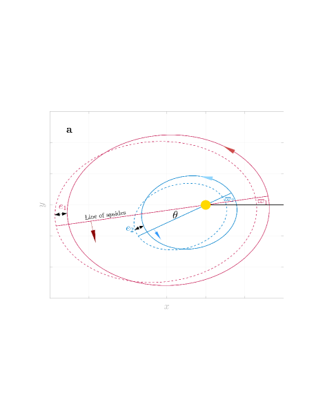
Figure 4: Schematic illustration of $g$ and $s$ modes for $N=3$ (for symbols and notation, see Table 1 and Fig. 2). Note that there is generally no simple one-to-one relationship between eigenmode and a single planet (see text). (a) $g$ modes (inclinations zero, viewed from ecliptic north; $\theta=\mbox{$\varpi$}_{2}-\mbox{$\varpi$}_{1}$). The apsidal precession is prograde (counterclockwise) in the same direction as the orbital motion (light blue and red arrows). (b) $s$ modes. The nodal precession is retrograde (clockwise) in the opposite direction as the orbital motion (light blue and red arrows). The orbit normals $\mbox{$\mbox{\boldmath$n$}$}_{i}$ hence describe a precessional/nutational motion (here about the $z$-axis).

The secular frequencies of the solar system naturally split into $g$ and $s$ modes, which are loosely related to the apsidal and nodal precession of the orbits, respectively (see Fig. 4). The $g$ and $s$ frequencies are constant in quasi-periodic systems but vary over time in chaotic systems and as such are critical for understanding the long-term behavior of the solar system. The $g$’s and $s$’s may be obtained by spectral analysis of the classic variables for each planet (see Fig. 5 and Table 3):

$$h=e\sin(\mbox{$\varpi$})\quad \quad k=e\cos(\mbox{$\varpi$})$$ ; (4)

$$p=\sin(I/2)\ \sin\mbox{$\Omega$}\quad \quad q=\sin(I/2)\ \cos\mbox{$\Omega$}\ ;$$ ; (5)

for $e$, $I$, $\varpi$, and $\Omega$, see Figs. 2, 4, and Table 1. In the Laplace-Lagrange solution, the $h,k,p$, and $q$ can be written as simple trigonometric sums with constant $g$’s and $s$’s (e.g., Murray and Dermott, 1999).

Keeping in mind the generally complex relation between individual planets and eigenmodes, the $g$ and $s$ modes may be schematically illustrated (see Fig. 4 for $N=3$). The $g$ modes involve variations in $e$ and $\varpi$, where $e$ usually varies between some extreme values (black double arrows, Fig. 4a) and $\varpi$ characterizes the apsidal precession; $\varpi$ may librate (oscillate) or circulate for solar system orbits. In the linear system and for a simple eigenmode-planet relationship, the time average $\langle\mbox{$\varpi$}_{i}\rangle$ may be written as $\langle\mbox{$\varpi$}_{i}\rangle\simeq g_{i}t$, or $\langle\dot{\mbox{$\varpi$}}_{i}\rangle\simeq g_{i}$ (where “dot” denotes the time derivative). The planetary $g_{i}$’s ($i=1,\ldots,8$) are positive (see Table 3), hence for circulating $\varpi$, the time-averaged apsidal precession is prograde (i.e., in the same direction as the orbital motion, see large arrows in Fig. 4a). The frequency $g_{9}$ (dominated by Pluto) is negative (Table 3). Importantly, however, the values and signs of the solar system’s fundamental frequencies are not deduced from the motion of individual planets, but from the eigenmode analysis of the full system.

Figure 5: Time series analysis of (a) $k$ and (b) $q$ for Earth (see Eqs. (4) and (5)) to extract solar system secular (or fundamental) frequencies from numerical integrations (solution ZB18a). Time interval: [$-$20 0] Myr. $\cal F$ = Fast-Fourier Transform (FFT). Vertical dashed lines indicate frequencies (see Table 3). Note that $s$ frequencies (b) are negative (retrograde nodal precession). Also note significant side peaks due to ($g_{4}$$-$$g_{3}$) around the main peaks $s_{3}$ and $s_{4}$. Side peaks around $g_{3}$ and $g_{4}$ in (a) are also present due to ($s_{4}$$-$$s_{3}$), illustrating the interaction of $g$ and $s$ modes. For a ratio $\mbox{($s_{4}$$-$$s_{3}$)}:\mbox{($g_{4}$$-$$g_{3}$)}=\$2:1, $s_{4}-\mbox{($g_{4}$$-$$g_{3}$)}=s_{3}+\mbox{($g_{4}$$-$$g_{3}$)}$.

Table 3: Solar system secular (or fundamental) frequencies (arcsec y^-1 = ^′′ y^-1)^a and periods (y) from ZB18a. Interval: [$-$20 0] Myr.

#	$g$	$T_{g}$	$s$	$T_{s}$
	b(′′ y-1)	(y)	(′′ y-1)	(y)
1	5.5821	232,170	$-$5.6144	230,837
2	7.4559	173,821	$-$7.0628	183,498
3	17.3695	74,613	$-$18.8476	68,762
4	17.9184	72,328	$-$17.7492	73,017
5	4.2575	304,404	0.0000	$-$
6	28.2452	45,884	$-$26.3478	49,188
7	3.0878	419,719	$-$2.9926	433,072
8	0.6736	1,923,992	$-$0.6921	1,872,457
9	$-$0.3494	3,709,721	$-$0.3511	3,691,356

^a 1 arcsec = 1/3600 of a degree.
^b Frequency conversion from kyr^-1 to arcsec y^-1 is ($\times 3600\cdot 360/1000=1296$).

The lines of apsides of two orbits coincide, i.e., their perihelia are aligned, for $\theta=\mbox{$\varpi$}_{2}-\mbox{$\varpi$}_{1}=2\pi\cdot n$, where $n$ is an integer (see Fig. 4a), or in the simple, linear system at $(g_{2}-g_{1})t=2\pi\cdot n$, i.e., at a frequency ($g_{2}$$-$$g_{1}$). Thus, one might expect that a major component in a planet’s orbital eccentricity spectrum occurs at the difference between two secular frequencies (relative motion). Indeed, the highest power in, e.g., Earth’s recent orbital eccentricity spectrum occurs at about $3.2~{}\mbox{${}^{\prime\prime}${\,}y\mbox{${}^{-1}$}}$ (arcsec y^-1, see Table 4), or a period of $\sim$405 kyr (see Fig. 6). It turns out that this frequency is associated with ($g_{2}$$-$$g_{5}$); the values given in Table 3 yield $\mbox{($g_{2}$$-$$g_{5}$)}=7.4559-4.2575=3.1984$ ^′′ y^-1, or 405 kyr. The ($g_{2}$$-$$g_{5}$) cycle is also called long eccentricity cycle (see Section 2.1.2) and represents the most stable $g$ mode combination term in Earth’s eccentricity spectrum in the recent past (although for deep time, see Zeebe and Lantink, 2024a). The various combinations of ($g_{i}$$-$$g_{j}$) and ($s_{i}$$-$$s_{j}$) relevant for Earth’s orbital eccentricity and inclination are discussed in Sections 2.1.4 and 2.4.

The $s$ modes involve variations in $I$ and $\Omega$, where $I$ usually varies between some extreme values (black double arrows, Fig. 4b) and $\Omega$ characterizes the nodal precession; $\Omega$ may librate or circulate. In the simple, linear system, the time average $\langle\mbox{$\Omega$}_{i}\rangle$ may be written as $\langle\mbox{$\Omega$}_{i}\rangle\simeq s_{i}t$, or $\langle\dot{\mbox{$\Omega$}}_{i}\rangle\simeq s_{i}$. The planetary $s_{i}$’s are negative (see Table 3), hence for circulating $\Omega$, the time-averaged nodal precession is retrograde (i.e., in the opposite direction as the orbital motion, see large arrows in Fig. 4b). Given conservation of total angular momentum ($L$), there exists an invariable plane perpendicular to $L$, which is fixed in space. It follows that one of the $s$ frequencies is zero ($s_{5}$, see Table 3). Thus, the $p$ and $q$ solutions behave slightly different than the $h$ and $k$ solutions (see Eqs. (4) and (5)). The eccentricity of an orbit introduces a reference line and hence an asymmetry into the problem for the $g$ modes ($h,k$), which is not the case for the $s$ modes ($p,q$). For the latter, the mutual inclination between, say, two orbits matters, not the absolute inclination relative to an arbitrary reference plane (Murray and Dermott, 1999).

2.1.4 Frequency Combination Terms: Eccentricity & Obliquity-Modulation

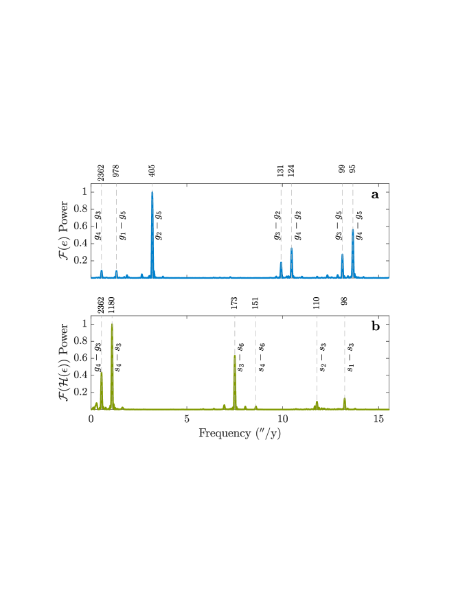
Figure 6: (a) FFT of Earth’s orbital eccentricity in the recent past ($\mbox{$\cal F$}(e)$). Interval: [$-$20 0] Myr. (b) FFT of the Hilbert transform of Earth’s obliquity ($\mbox{$\cal F$}(\mbox{$\cal H$}(\mbox{$\epsilon$}))$. Spectral power is normalized to maximum power. Numbers above panels indicate periods in kyr.

As discussed above, major components (terms) in relevant orbital parameter spectra usually occur at the difference between pairs For instance, the main eccentricity terms in the recent past (405 kyr and $\sim$100 kyr) are due to combination pairs of $g$ frequencies (see Fig. 6a and Table 4). Importantly, the $\sim$100 kyr band is actually composed of four individual frequencies, which, in geologic sequences, are identifiable separately however only in high-quality cyclostratigraphic records. The $g$-frequency combination terms that dominate orbital eccentricity (Fig. 3) are directly accessible through time series analysis of eccentricity (here FFT, $\mbox{$\cal F$}(e)$, Fig. 6). Note that in general, there is no analogous relationship between $s$-frequency combinations and inclination, again due to the dependence of inclination on the reference frame (see Section 2.1.2). A natural choice for extracting $s$-frequency combinations from inclination would be the invariant frame. However, orbital elements in the invariant frame are not universally provided by $\cal AS$s. Moreover, compared to eccentricity, there is also no equivalent expression of inclination in stratigraphic sequences that could be used for practical purposes.

A more useful approach for extracting $s$-frequency combinations from $\cal AS$s is analyzing the amplitude modulation of obliquity. This approach also makes practical sense because obliquity and its AM are often expressed in cyclostratigraphic records. To obtain the AM frequency terms of obliquity from $\cal AS$s, we first extract the envelope of obliquity by applying the Hilbert transform, $\cal H$($\epsilon$) (see also Fig. 12) and then apply FFT ($\mbox{$\cal F$}(\mbox{$\cal H$}(\mbox{$\epsilon$}))$, Fig. 6b and Table 4). The strongest obliquity AM terms in the recent past are ($s_{4}$$-$$s_{3}$) and ($s_{3}$$-$$s_{6}$), which are discussed in more detail in Section 2.4. The next highest peak is due to $g$ modes (not $s$ modes), i.e., the combination ($g_{4}$$-$$g_{3}$), which may be surprising if one expects only $s$ terms to appear in the obliquity AM spectrum. However, as shown above, significant ($g_{4}$$-$$g_{3}$) side peaks are present around $s_{3}$ and $s_{4}$ (Fig. 5). In turn, the combination of the main- and side peaks then lead to significant power at the beat frequency ($g_{4}$$-$$g_{3}$) in the obliquity AM spectrum. The interaction of $g$ and $s$ modes, i.e., $g$ frequencies appearing in $q$’s spectrum and $s$ frequencies appearing in $k$’s spectrum (see Eqs. (4), (5), and Fig. 5) illustrate the non-linear behavior of solar-system dynamics (in the linear system, the $g$ and $s$ modes are decoupled and independent of each other). In fact, ($s_{4}$$-$$s_{3}$) and ($g_{4}$$-$$g_{3}$) are currently in a so-called 2:1 resonance state (periods of $\sim$1.2 and $\sim$2.4 Myr, Table 4), which is a major contributor to long-term solar-system chaos (see Sections 2.3 and 2.4).

Table 4: Frequency terms (arcsec y^-1 = ^′′ y^-1)^a and periods (kyr) based on $g$ and $s$ frequencies in ZB18a (interval: [$-$20 0] Myr, see Table 3).

Term	Short-	Freq.	Period	Expressed
	hand	b(′′ y-1)	c(kyr)	in
($g_{4}$$-$$g_{3}$)	$g_{43}$	0.5487	2362	Ecc.& Oblq.
($g_{1}$$-$$g_{5}$)	$g_{15}$	1.3246	978	Eccentricity
($g_{2}$$-$$g_{5}$)	$g_{25}$	3.1984	405	Eccentricity
($g_{3}$$-$$g_{2}$)	$g_{32}$	9.9137	131	Eccentricity
($g_{4}$$-$$g_{2}$)	$g_{42}$	10.4624	124	Eccentricity
($g_{3}$$-$$g_{5}$)	$g_{35}$	13.1121	99	Eccentricity
($g_{4}$$-$$g_{5}$)	$g_{45}$	13.6609	95	Eccentricity
		——
($s_{4}$$-$$s_{3}$)	$s_{43}$	1.0983	1180	Obliquity-AM
($s_{3}$$-$$s_{6}$)	$s_{36}$	7.5003	173	Obliquity-AM
($s_{4}$$-$$s_{6}$)	$s_{46}$	8.5986	151	Obliquity-AM
($s_{2}$$-$$s_{3}$)	$s_{23}$	11.7847	110	Obliquity-AM
($s_{1}$$-$$s_{3}$)	$s_{13}$	13.2331	98	Obliquity-AM

^a 1 arcsec = 1/3600 of a degree.
^b Frequency conversion from kyr^-1 to arcsec y^-1 is ($\times 3600\cdot 360/1000=1296$).
^c Uncertainties in ($g_{4}$$-$$g_{3}$) and ($s_{4}$$-$$s_{3}$) periods from spectral analysis may be estimated as $\pm 40$ kyr and $\pm 10$ kyr (Zeebe, 2022).

2.2 The so-called “Metronomes”

The term astrochronological metronome usually refers to a prominent and exceptionally stable frequency in Earth’s orbital parameters that may be widely used to construct accurate chronologies. Importantly, for the frequencies to be of use in practical applications requires both frequency and amplitude to be stable. The eccentricity term ($g_{2}$$-$$g_{5}$) ($\sim$405 kyr in the recent past) and the inclination term ($s_{3}$$-$$s_{6}$) ($\sim$173 in the recent past) have been labeled the eccentricity- and inclination metronome, respectively (Laskar, 2020). However, Zeebe and Lantink (2024a) have recently shown that ($g_{2}$$-$$g_{5}$) can become unstable on long time scales, which compromises the 405-kyr cycle’s reliability beyond several hundred million years in the past. The term ($s_{3}$$-$$s_{6}$) is also unreliable, yet on even shorter time scales. For example, analysis of the obliquity modulation (illustrated in Fig. 6) of the solution ZB18a shows that the dominant term involving $s_{6}$ across the interval $-$66 to $-$56 Myr is ($s_{4}$$-$$s_{6}$), and not ($s_{3}$$-$$s_{6}$). Note that ZB18a has been geologically constrained to $-$66 Myr, which includes the interval in question from $-$66 to $-$56 Myr (see Zeebe and Lourens, 2022b, and Table 5). Shifts in the dominant terms are due to changes in $s_{3}$ and $s_{4}$, which are known to be variable beyond $\sim$50 Myr (see Fig. 6 of Zeebe and Lourens (2022b)). As a result, the dominant period involving $s_{6}$ may shift to $\sim$151 kyr or even alternate over time between $\sim$173 and $\sim$151 kyr. In summary, the current evidence does not support the notion of generally stable and prominent metronomes for universal use in astrochronology and cyclostratigraphy. The term ($s_{3}$$-$$s_{6}$) is reliable only over the past 50 Myr or so, an interval over which the secular frequencies appear stable anyway. The term ($g_{2}$$-$$g_{5}$) is more stable but cannot be taken for granted beyond several 100 Myr due to solar system chaos.

2.3 Solar System Chaos

Large-scale dynamical chaos is an inherent characteristic of the solar system and fundamental to understanding the behavior of astronomical solutions and their limitations, which is described below. First, an example of a simple analog mechanical system is introduced to illustrate some basic aspects of chaos.

2.3.1 The Driven Pendulum: Poincaré Section

Fundamental contributions to the theory of dynamical systems (including the gravitational three-body problem and the solar system) were made by Henri Poincaré (1854-1912), whose work laid the foundations of chaos theory. Poincaré wrote: “It may happen that small differences in the initial conditions produce very great ones in the final phenomena. A small error in the former will produce an enormous error in the latter. Prediction becomes impossible $\ldots$” (Poincaré, 1914). The sensitivity to small differences in initial conditions or small perturbations is a key element of chaotic systems.

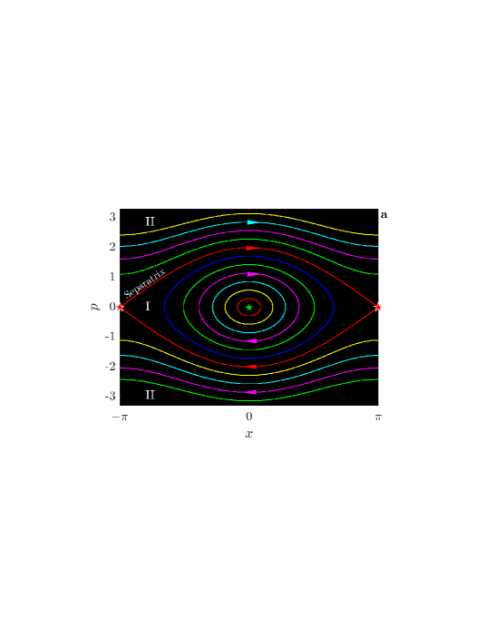
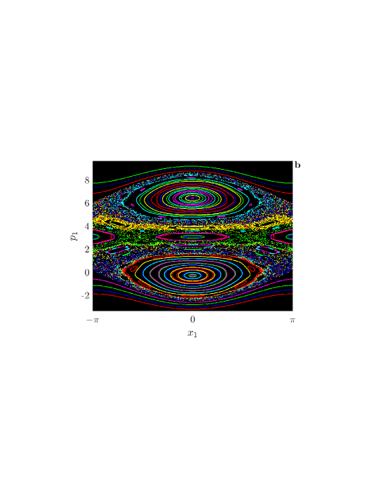
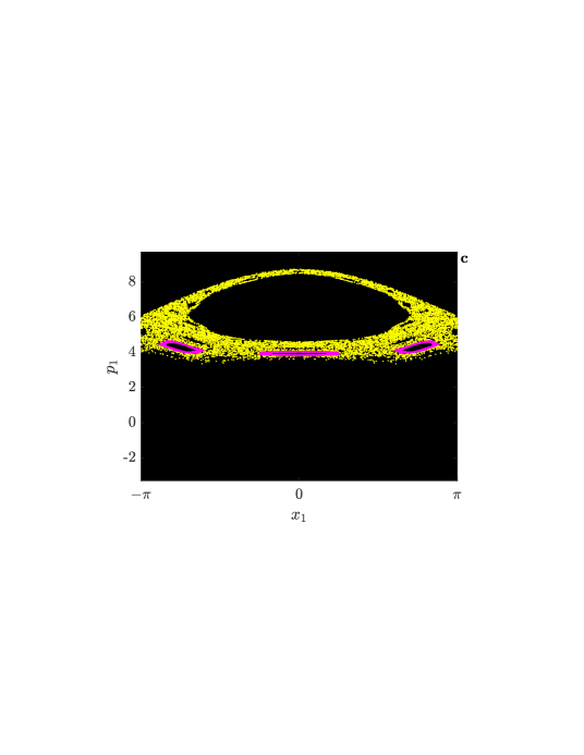
Figure 7: (a) Phase diagram ($x=$ position/angle, $p=$ momentum) of the simple rigid pendulum (units normalized). Green/red stars: stable/unstable fixed points (modulo $2\pi$). Color coding indicates phase space trajectories for each set of initial conditions ($x^{0},p^{0}$), $N=16$, from which the equations of motion are numerically integrated. (b) Poincaré section (aka surface of section) of the driven rigid pendulum ($N=64$ initial conditions) (simplified Hamiltonian, see Chapter 6, Morbidelli, 2002). (c) Same as (b) for $N=2$, $p^{0}_{1}$ differs by $10^{-6}$.

A simple mechanical system often used to illustrate such behavior is the driven rigid pendulum (e.g., Chirikov, 1979; Lichtenberg and Lieberman, 1983; Murray and Holman, 2001; Morbidelli, 2002). Consider first a simple rigid pendulum in a gravitational field with angle $x$ to the vertical (equivalent to position) and momentum $p=ml\dot{x}$, where $m$ and $l$ are its effective mass and length, respectively (for phase diagram, see Fig. 7a). For small to moderate energies (regime I), the pendulum librates around the equilibrium point ($x,p$) = (0,0), representing a single oscillator. The trajectories originating in regime I are considered to be in resonance (Murray and Holman, 2001). For large energies (regime II), the pendulum rotates clockwise ($p<0$) or counterclockwise ($p>0$). The structure that separates the two regimes is called the separatrix (Fig. 7a). For initial conditions starting on the separatrix, the pendulum approaches the unstable fixed point (Fig. 7a, red star) as $t\rightarrow\infty$ (upright position). The motion of the pendulum starting in the vicinity of initial conditions ($x^{0},p^{0}$) in regime I or II far from the separatrix is quite simple. Starting at neighboring points in regime I will lead to libration, whereas starting at neighboring points in regime II will lead to rotation. However, for ($x^{0},p^{0}$) very close to the separatrix, neighboring starting points may lead to fundamentally different outcomes governing their motion, e.g., libration or rotation. In chaotic systems, one may think of the separatrix as “the cradle of chaos” (Murray and Holman, 2001).

While the motion of the simple rigid pendulum is non-chaotic (universally), this is not the case for the driven rigid pendulum (Fig. 7b). Imagine a driven pendulum by, for instance, applying a periodic force (torque) to the pendulum or periodically moving its pivot point, which results in the interaction of two oscillators (pendulum and pivot). Instead of two phase-space variables for the simple rigid pendulum, four variables are now needed to describe the motion, say $x_{1},p_{1},x_{2}$ and $p_{2}$. Thus, the phase space is four-dimensional (4D), which cannot be fully represented in 2D. To visualize the dynamics, a lower-dimensional phase diagram is often constructed, called a Poincaré section, or surface of section. For example, for the driven pendulum, one may select the surface ($x_{1},p_{1}$), with $x_{2}$ perpendicular to the surface, and plot ($x_{1},p_{1}$) only when $x_{2}=0$, i.e., at times when the phase trajectory intersects the ($x_{1},p_{1}$) plane (see Fig. 7b). Usually, an additional condition is specified for $p_{2}$, e.g., $p_{2}>0$. One can think of a Poincaré section as a stroboscopic image of the trajectory’s time evolution in phase space (Morbidelli, 2002).

The critical ingredient for chaotic dynamics are overlapping resonances. For illustration, consider the single resonance (Fig. 7a, one ‘cat’s eye’) and the two resonances (Fig. 7b, two ‘cat’s eyes’ atop one another). For certain parameter values of the driven pendulum (e.g., driving frequency close to the natural pendulum frequency), the two resonances are close enough to overlap (Fig. 7b, around $p_{1}=\pi$). The structures of certain phase space regions still appear relatively simple, such as in the vicinity of the resonances centered at (0,0) and (0,$\mbox{$\sim$}{2}\pi$) and for large $|p_{1}|$, corresponding to regimes I and II, respectively (Fig. 7a). The motion in these regions may be restricted to invariant (stable) tori, or KAM tori (for summary, see Morbidelli, 2002). However, for certain initial conditions, chaotic phase space regions appear, expressed in the Poincaré section as disordered sets of scattered points (see, e.g., transition areas between regions of libration and rotation, Fig. 7b and c). In chaotic regions of the phase space, nearby trajectories diverge exponentially, characterized by their Lyapunov exponent (see Section 1). As a result, the system is sensitive to small differences in initial conditions and small perturbations. For example, two trajectories of the driven pendulum ($x^{0}_{1},p^{0}_{1})=(0,\mbox{$\sim$}{3.82})$ that initially differ by only $10^{-6}$ in $p^{0}_{1}$ rapidly diverge and occupy different (separate) regions of the phase space (Fig. 7c). Prediction becomes impossible, as Poincaré had pointed out.

The driven pendulum serves as a useful illustration for various properties of chaotic systems, including the sensitivity to initial conditions. The full orbital dynamics of, for instance, the solar system, are of course substantially more complex (see below). Nevertheless, key elements such as the sensitivity to initial conditions and the overlap of resonances are also critical in solar system dynamics (note that for secular resonances, the $g$ and $s$ frequencies are involved, see Section 2.1.3). For example, it was recently discovered that Earth’s long eccentricity cycle can be become unstable on long time scales due to the resonance $(g_{1}-g_{2})+(s_{1}-s_{2})\simeq 0$ (see Zeebe and Lantink, 2024a)

2.3.2 Solar System: Time Scales and Limitations

As mentioned above, large-scale dynamical chaos is an inherent property of the solar system, which has been independently confirmed in various numerical studies (e.g., Sussman and Wisdom, 1988; Laskar, 1989; Ito and Tanikawa, 2002; Morbidelli, 2002; Varadi et al., 2003; Batygin and Laughlin, 2008; Zeebe, 2015; Brown and Rein, 2020; Hernandez et al., 2022; Abbot et al., 2023; Zeebe and Lantink, 2024a). For observational studies, see, e.g., Ma et al. (2017); Westerhold et al. (2017); Olsen et al. (2019); Zeebe and Lourens (2019). Dynamical chaos affects the secular frequencies $g_{i}$ and $s_{i}$ (see Section 2.1.3), where the terms ($g_{4}$$-$$g_{3}$) and ($s_{4}$$-$$s_{3}$), for instance, show chaotic behavior already on a 50-Myr time scale. As a result, astronomical solutions diverge around $t=\pm 50$ Myr, which fundamentally prevents identifying a unique solution on time scales $\stackrel{{\scriptstyle>}}{{\sim}}\$10⁸ y (Laskar et al., 2004; Zeebe, 2017; Zeebe and Lourens, 2019). The quest for a single deterministic solution, which conclusively describes the solar system’s evolution for all times (in the spirit of Laplace’s demon, see Laplace, 1951), must therefore be regarded as quixotic. In fact, long-term predictability is fundamentally unachievable (Poincaré, 1914). The chaos not only severely limits our understanding and ability to reconstruct and predict the solar system’s history and long-term future, it also imposes fundamental limits on geological and astrochronological applications such as developing a fully calibrated astronomical time scale beyond $\sim$50 Ma, including the SEC (for recent efforts, see Zeebe and Lourens, 2019, 2022b; Kocken and Zeebe, 2024).

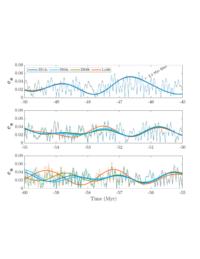
Figure 8: Earth’s orbital eccentricity ($e_{\Earth}$) from different OS: ZB18a (Zeebe and Lourens, 2019), ZB20a and ZB20b (Zeebe and Lourens, 2022b), and La10b (Laskar et al., 2011). The 2.4-Myr filter is sensitive to the amplitude modulation of eccentricity, with minima corresponding to a reduced amplitude of the short eccentricity cycle, aka very long eccentricity nodes (VLN).

The limits imposed by dynamical chaos on astronomical calculations may be illustrated by comparing Earth’s eccentricity ($e_{\Earth}$) from different OS prior to $-50$ Myr (Fig. 8). As an example, we select three of the most current and up-to-date OS (ZB18a, ZB20a, and ZB20b), which have been constrained by geologic data up to an age of 66 Ma (see Section 2.5 and Zeebe and Lourens (2019, 2022b)). ZB18a, ZB20a, and ZB20b use identical initial conditions but feature slightly different $J_{2}$ values (for details, see Section 2.6 and Zeebe, 2017; Zeebe and Lourens, 2019, 2022b) and number of asteroids included in the simulation. Visually, $e_{\Earth}$ calculated based on these three OS is nearly identical back to ca. $-58$ Myr but diverge quickly beyond that time, as highlighted by a 2.4-Myr filter (Fig. 8). The 2.4-Myr filter is sensitive to the amplitude modulation of eccentricity, aka very long eccentricity nodes (VLN), with frequency ($g_{4}$$-$$g_{3}$). Of the La10x solutions, La10b and La10c appear to provide the best match with geological data to $\sim$58 Ma, but not beyond (Westerhold et al., 2017; Zeebe and Lourens, 2019, 2022b). La10b, for example, exhibits a large 100-kyr amplitude just prior to $-59$ Myr (see Fig. 8), while ZB18a and ZB20a exhibit small 100-kyr amplitudes (VLNs). Features such as VLNs are important criteria to distinguish between different OSs based on geologic data (Westerhold et al., 2017; Zeebe and Lourens, 2019, 2022b).

The example using $e_{\Earth}$ based on different OSs (Fig. 8) again illustrates one key feature of dynamical chaos, i.e., the sensitivity to tiny perturbations or small differences in initial conditions (see Section 2.3.1). For example, the masses of the largest asteroids are roughly ten billion times smaller than the solar mass (which represents the magnitude of the first-order gravitational interaction). Yet, changing the number of asteroids included in the simulation drives the solutions apart beyond ca. $-58$ Myr (Fig. 8). Small differences in trajectories grow exponentially, with a time constant (Lyapunov time, see Section 1) for the inner planets of $\sim$3-5 Myr estimated numerically (Laskar, 1989; Varadi et al., 2003; Batygin and Laughlin, 2008; Zeebe, 2015). For example, a difference in initial position of $1$ cm grows to $\sim$1 AU (= 1.496$\times 10^{11}$ m) after 90-150 Myr, which makes it fundamentally impossible to predict the evolution of planetary orbits accurately beyond a certain time horizon.

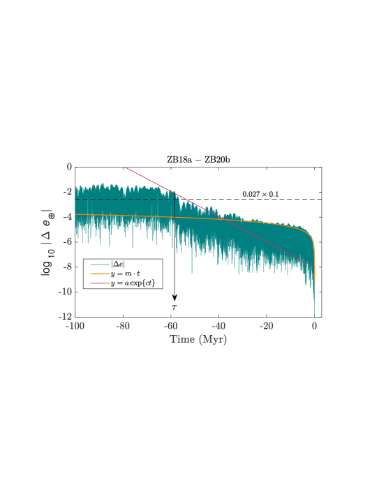
Figure 9: Difference in Earth’s orbital eccentricity on a log-$y$ scale, $\log_{10}|\mbox{$\Delta e_{\Earth}$}|$, between the solutions ZB18a and ZB20b over the past 100 Myr. The arrow indicates the divergence time $\tau$, when max$|\mbox{$\Delta e_{\Earth}$}|$ irreversibly crosses $\sim$10% of mean $e_{\Earth}$ ($\mbox{$\sim$}0.027\times 0.1$, dashed horizontal line). Orange curve: simple fit function with linear growth in $|\mbox{$\Delta e_{\Earth}$}|$. Red line: exponential growth in $|\mbox{$\Delta e_{\Earth}$}|$ (linear on log-$y$ scale) with a Lyapunov time of 4.3 Myr (see text).

In contrast to the limitations discussed above (largely due to unstable terms such as ($g_{4}$$-$$g_{3}$) and ($s_{4}$$-$$s_{3}$)), another frequency term appears more promising as it shows more stable behavior. For example, it has hitherto been assumed that ($g_{2}$$-$$g_{5}$) was practically stable in the past and has been suggested for use as a “metronome” in deep-time geological applications, i.e., far exceeding 50 Ma (Laskar et al., 2004; Kent et al., 2018; Spalding et al., 2018; Meyers and Malinverno, 2018; Montenari, 2018; Lantink et al., 2019; De Vleeschouwer et al., 2024). The ($g_{2}$$-$$g_{5}$) cycle, which is the dominant term in Earth’s orbital eccentricity in the recent past ($\sim$405 kyr, see Fig. 6) may thus have been regarded as an island of stability in a sea of chaos. However, as mentioned above, ($g_{2}$$-$$g_{5}$) can als become unstable over long time scales (Zeebe and Lantink, 2024a).

2.3.3 Divergence Time $\tau$

The action of chaos on Earth’s orbital evolution may be illustrated by the difference between two eccentricity solutions ($|\mbox{$\Delta e_{\Earth}$}|$), say plotted on a log scale (Fig. 9). Starting at $t_{0}$ and integrating backwards in time, integration errors dominate initially. Integration errors usually grow polynomially (for angle-like variables), here $\propto\ t$ and dominant for $t\ \raisebox{-2.15277pt}{$\stackrel{{\scriptstyle>}}{{\sim}}\ $}-40$ Myr (see orange line, Fig. 9; note that a function linear in $t$ appears non-linear on a log scale). Ultimately, the divergence of trajectories is dominated by exponential growth ($t\ \raisebox{-2.15277pt}{$\stackrel{{\scriptstyle<}}{{\sim}}\ $}-40$ Myr), which is indicative of chaotic behavior (red line, Fig. 9). For $t\ \raisebox{-2.15277pt}{$\stackrel{{\scriptstyle<}}{{\sim}}\ $}-60$ Myr, the solutions have completely diverged and their difference may reach the maximum of $\sim$0.06 ($\max|\mbox{$\Delta e_{\Earth}$}|$ no longer increases, see Fig. 8). The difference between two orbital solutions may be tracked by the divergence time $\tau$, i.e., the time interval after which the absolute difference in Earth’s eccentricity ($|\mbox{$\Delta e_{\Earth}$}|$) irreversibly crosses $\sim$10% of mean $e_{\Earth}$ ($\mbox{$\sim$}0.027\times 0.1$, Fig. 9). Simply put, $\tau$ represents the time interval beyond which the solutions no longer agree. The divergence time is largely controlled by the Lyapunov time, although the two are different quantities.

2.3.4 Chaos and Inapplicability of Basic Statistics

Chaos introduces elements of inherent unpredictability into dynamical systems, which generally leads to fundamental unaccountability in terms of basic statistics. Note that the following is not a criticism of statistics, but rather of attempts to apply basic statistical concepts to chaotic patterns, which may arise from a misunderstanding of the dynamics of the system. For instance, consider a dynamical system parameter, which, when increased by a small amount $\delta$ produces a change in a system variable by an amount $X$. If $\delta$ is now varied incrementally, one may expect that $X$ is a function of $\delta$ (linear or nonlinear) that somehow scales with the size of $\delta$. However, this is generally not the case in chaotic systems (see Section 2.3.1). As an example, consider the solar system in which Earth’s initial position ($x$-coordinate) is varied by $\mbox{$\delta$}=\mbox{$\Delta$}x_{0}$. The system is then integrated for different $\mbox{$\Delta$}x_{0}$ over 100 Myr and the differences in Earth’s orbital eccentricity $e_{\Earth}$ are evaluated (Zeebe, 2023), say tracked using the divergence time $\tau$ (see Fig. 10). Note that $\tau$ is not a measure of accuracy or inaccuracy.

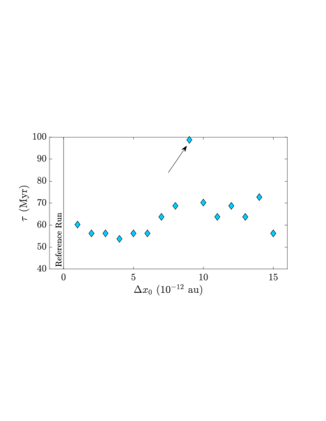
Figure 10: Ensemble integrations with orbitN (general relativity, $J_{2}$, and the lunar contribution turned off, see Zeebe, 2023). Earth’s initial $x$-coordinate is perturbed by a small $\mbox{$\Delta$}x_{0}=1\mbox{$\times 10^{-12}$}$ au ($\sim$15 cm), relative to the corresponding reference run ($\mbox{$\Delta$}x_{0}=0$ au). The difference between two orbital solutions $i$ and $j$ may be tracked using the divergence time $\tau$ (see Fig. 9 and Zeebe, 2017). The run resulting in the largest $\mbox{$\tau$}\simeq 100$ Myr (arrow) is not a mistake, numerical error, or “outlier” (see text).

First, there is no systematic relationship between $\tau$ and $\mbox{$\Delta$}x_{0}$ that somehow scales with the size of $\mbox{$\Delta$}x_{0}$. Second, the run resulting in the largest $\mbox{$\tau$}\simeq 100$ Myr (see arrow) is not a mistake, numerical error, or “outlier” that can therefore be excluded (the run was carefully examined). The run is a proper solution of the system, illustrating the unpredictability and unaccountability of chaotic systems in terms of basic statistics. For example, values that fall outside two or three sigma from the mean are often considered outliers, which is not applicable here. One important corollary is that it is generally not possible to “tune” or “fit” astronomical solutions to geological data. The best that can probably be done is to “constrain” astronomical solutions by geological data. In other words, to create large ensembles of solutions via parameter variations and select/discard those solutions that show good/poor agreement with the data (Zeebe and Lourens, 2019, 2022b).

As outlined in the preceding sections, solar system chaos is key to understanding the limitations imposed on orbital solutions by chaotic dynamics, resonances, the behavior of ensemble integrations, and more. Chaos also causes critical changes in the amplitude modulation of orbital forcing signals, which, if expressed in cyclostratigraphic sequences, can be used to reconstruct the solar system’s chaotic history. Elements of amplitude (and frequency) modulation are covered in Section 2.4.

2.4 Amplitude & Frequency Modulation (AM & FM)

Amplitude and frequency modulation of orbital forcing signals is similar to AM/FM techniques used in radio broadcasting. Schematically, the carrier signal (high frequency) is modulated, resulting either in slow modulation of the amplitude (AM) or frequency (FM), see Fig. 11. For example, the astronomical carrier frequency may be precession, eccentricity, or obliquity, while the AM frequency (or “beat”, see below) may be eccentricity or various combinations of ($g_{i}$$-$$g_{j}$) and ($s_{i}$$-$$s_{j}$), see Section 2.1.4. As described below, frequency modulation is less commonly used than amplitude modulation in astrochronology and cyclostratigraphy. Also, while there is a direct analogy between radio AM and astronomical forcing AM, the analogy is not straightforward for the FM case study discussed here (Section 2.4.2).

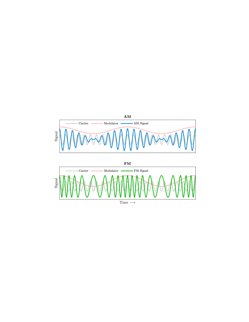
Figure 11: Schematic illustration of amplitude & frequency modulation (AM & FM).

2.4.1 AM

Amplitude modulation is frequently used in cyclostratigraphy because AM cycles are often expressed in geologic sequences (also called “beats” in analogy to beat frequencies in music). For example, the amplitude of climatic precession is modulated by eccentricity (in a very simple manner, i.e., eccentricity is the envelope of climatic precession, $\mbox{$\bar{p}$}=e\sin\mbox{$\bar{\omega}$}$, see Fig. 1). Also, the SEC’s amplitude is modulated by the LEC. Bundles of four SECs in the recent past (each $\sim$100 kyr, for details see Eq. (6)) represent one LEC (405 kyr, see Fig. 13a). On even longer time scales, the eccentricity amplitude is modulated by ($g_{4}$$-$$g_{3}$), which leads to very long eccentricity nodes (VLNs) with much reduced SEC amplitude and a recent period of $\sim$2.4 Myr (Fig. 12a). The spectrum of Earth’s orbital eccentricity is largely dominated by simple combinations of the $g$ frequencies $g_{2}$ to $g_{5}$ (see Tables 3 and 4). Thus, there is a simple relationship between, for instance, ($g_{4}$$-$$g_{3}$) and the other relevant $(g_{i}-g_{j})$ terms (individual SEC’s are $\sim$124, 131, 95, and 99 kyr):

($$g_{4} - g_{3} = (1/72.328-1/74.613)\mbox{${}^{-1}$}=2362~{}\mbox{kyr}$$)^-1 (6)

$$= (g_{42}-g_{32})\mbox{${}^{-1}$}=(g_{45}-g_{35})\mbox{${}^{-1}$}$$

$$\simeq (1/123.87-1/130.73)\mbox{${}^{-1}$}\simeq(1/94.87-1/98.84)\mbox{${}^{-1}$}\ .$$

Importantly, owing to chaotic dynamical behavior, the fundamental frequencies (and hence the beats) are not constant, but change over time. The changing VLN patterns beyond about $50$ Ma observed in cyclostratigraphic records are important criteria to distinguish between different orbital solution (Westerhold et al., 2017; Zeebe and Lourens, 2019, 2022b).

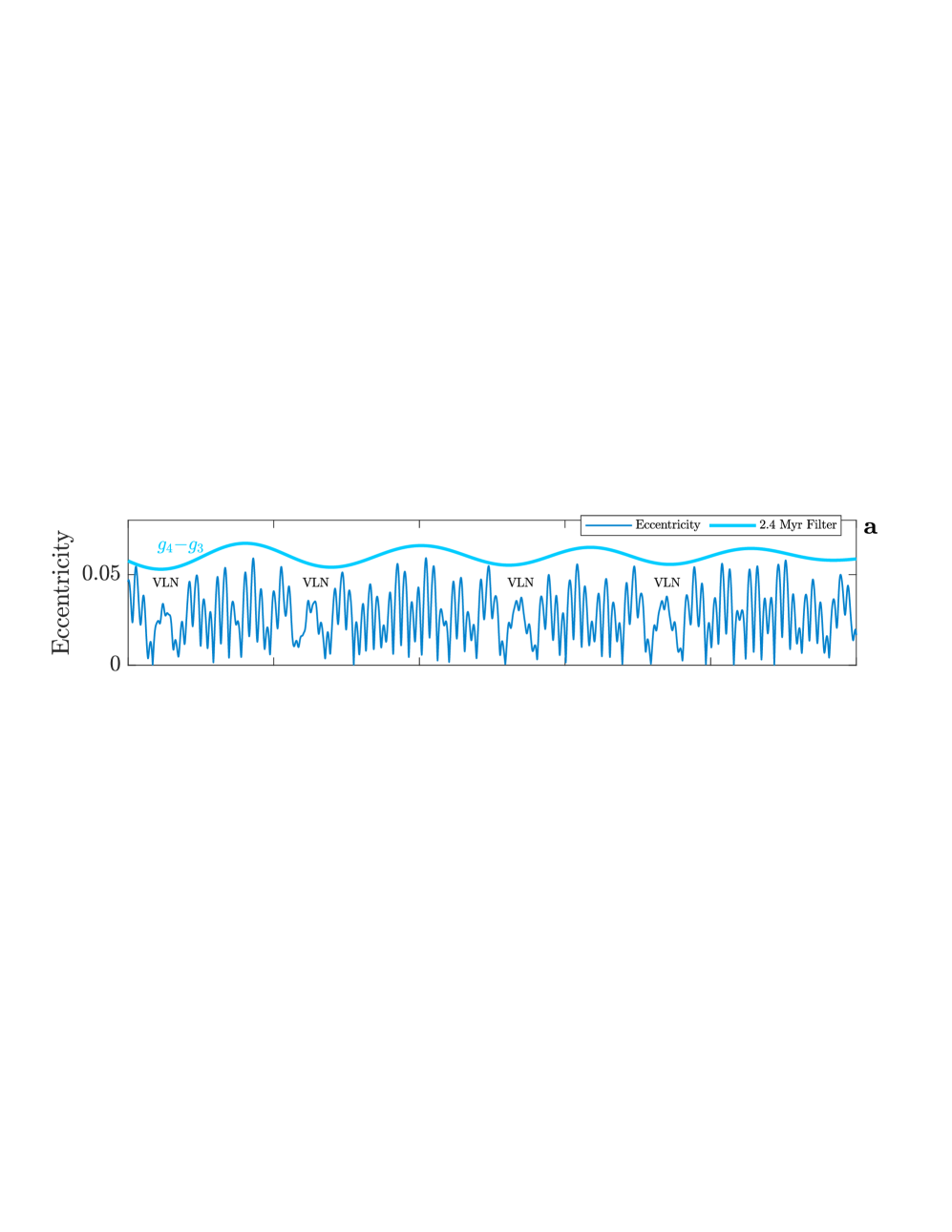
Figure 12: (a) Earth’s orbital eccentricity and $\sim$2.4 Myr filter corresponding to ($g_{4}$$-$$g_{3}$). VLN = very long eccentricity node. Filters are plotted using arbitrary amplitudes and vertical offsets. (b) Obliquity, its Hilbert transform $\cal H$($\epsilon$), $\sim$1.2 Myr filter of $\cal H$($\epsilon$) corresponding to ($s_{4}$$-$$s_{3}$), and 173 kyr filter of $\cal H$($\epsilon$) corresponding to ($s_{3}$$-$$s_{6}$).

As discussed above, there is no direct analogy between eccentricity and inclination (see Section 2.1.2). Similarly, the analogy between their amplitude modulations (i.e., between ($g_{i}$$-$$g_{j}$) terms and ($s_{i}$$-$$s_{j}$) terms) is limited as well. The orbital parameter closely related to inclination is obliquity, which is often expressed in cyclostratigraphic sequences. Thus, to examine the AM associated with ($s_{i}$$-$$s_{j}$) terms, it is helpful to examine the AM of obliquity (see Fig. 12b). Again, to do so, we first extract the envelope of obliquity by applying the Hilbert transform, $\cal H$($\epsilon$). The two largest peaks in $\cal H$($\epsilon$)’s spectrum are located at periods of $\sim$1.2 Myr and $\sim$173 kyr (see Fig. 6). The 1.2-Myr period corresponds to ($s_{4}$$-$$s_{3}$), which is currently in a 2:1 resonance with ($g_{4}$$-$$g_{3}$) (Section 2.1.4). On time scales beyond $\sim$50 Myr, the ($s_{4}$$-$$s_{3}$):($g_{4}$$-$$g_{3}$) ratio is subject to chaotic transitions and may exhibit a wide range of values on Gyr-time scale (Zeebe and Lantink, 2024b). The 173-kyr period corresponds to ($s_{3}$$-$$s_{6}$), which is significant in the recent past (e.g., Shackleton et al., 1999; Hinnov, 2000; Pälike et al., 2004), and has been suggested to be expressed in multiple proxy records of Mesozoic and Cenozoic age (for recent summary see, e.g., Huang et al., 2021). However, for records older than $\sim$50 Ma, the assumed assignment and period is ambiguous and hence problematic owing to the lack of generally stable and prominent metronomes or geochronometers, including ($s_{3}$$-$$s_{6}$) (see Section 2.2).

2.4.2 FM

Frequency modulation is less commonly used than amplitude modulation in cyclostratigraphic studies (for a few examples, see Herbert, 1992; Liu, 1995; Hinnov and Park, 1998; Rial, 1999; Hinnov, 2000; Zeeden et al., 2015; Laurin et al., 2016; Piedrahita et al., 2022). One major challenge for cyclostratigraphic applications is the conversion from stratigraphic depth to time. Variations in sedimentation rate that are not taken into account would perturb the frequency of recorded astronomical cycles (similar to the FM illustration shown in Fig. 11). Conversely, tuning of the stratigraphic record to an astronomical frequency would map any frequency modulation in the data to variations in sedimentation rate. These issues represent substantial obstacles to FM analyses of sedimentary data. Another potentially complicating factor regarding FM is that age-model tuning approaches may introduce systematic frequency modulations (e.g., Zeeden et al., 2015). Nevertheless, analysis of short eccentricity-related FM interference patterns in stratigraphic sequences can, for instance, be used to discern LEC minima and maxima from SEC records (e.g., Laurin et al., 2016; Piedrahita et al., 2022). The link between the LEC and SECs is of course due to the relationship between the $g$ frequencies and their involvement in Earth’s orbital eccentricity, $e_{\Earth}$ (see Sections 2.1.3 and 2.1.4). The strongest terms in $e_{\Earth}$’s spectrum in the recent past are the LEC ($g_{2}$$-$$g_{5}$) ($\sim$405 kyr) and the SECs ($g_{4}$$-$$g_{2}$) and ($g_{4}$$-$$g_{5}$) ($\sim$124 and 95 kyr, $E_{2}$ and $E_{3}$ for short) (see Figs. 6 and 13). The combination of the two SECs in turn yields the LEC ($E_{1}$):

$$(1/95-1/124)\mbox{${}^{-1}$}\simeq 405~{}\mbox{kyr}\ .$$ (7)

Narrow filters of $e_{\Earth}$ around 124 and 95 kyr show interference patterns that correlate with minima and maxima in $E_{1}$. For instance, $E_{2}$ and $E_{3}$ interfere constructively (in-phase) during $E_{1}$ maxima and destructively (out-of-phase) during $E_{1}$ minima (Fig. 13a and b). Note that LEC maxima and minima correlate with large and small SEC amplitudes, respectively. Evolutive Harmonic Analysis (EHA) of $e_{\Earth}$ reveals a chain pattern in the $E_{2}$-$E_{3}$ amplitude, where nodes (single amplitude and period) correspond to $E_{1}$ maxima and rings (split amplitudes and periods) to $E_{1}$ minima (see arrows and crosses, Fig. 13c). Thus, the SEC-FM interference patterns can be used to deduce LEC minima and maxima (Laurin et al., 2016).

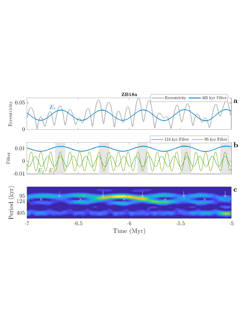
Figure 13: Illustration of eccentricity-related FM interference patterns. (a) Earth’s orbital eccentricity ($e_{\Earth}$) from solution ZB18a and 405-kyr filter ($E_{1}$). (b) Narrow filters of $e_{\Earth}$ around 124 ($E_{2}$) and 95 kyr ($E_{3}$). Gray bars mark intervals of $E_{2}$-$E_{3}$ constructive (in-phase) interference. Blue: scaled and offset 405-kyr filter from (a). (c) Evolutive Harmonic Analysis (EHA) of $e_{\Earth}$ (showing amplitude, not spectral power) using astrochron (Meyers, 2014). Arrows and crosses: nodes and rings in $E_{2}$-$E_{3}$ amplitude corresponding to maxima and minima in $E_{1}$, respectively (see (a)).

2.5 Up-to-Date Orbital Solutions

As described above, there is a long history of OSs — yet only a few are up-to-date and should be employed in current and future applications, which has not been the case in many recent applications, indicating confusion about proper use of OSs (see remark at the end of this section). For the time span from $-300$ to 0 Myr, we recommend the solutions ZB18a and ZB20x, which have been constrained by geologic data up to an age of 66 Ma (see Table 5). Importantly, significantly beyond the geologically constrained intervals, or the solution’s validity range, the OSs are unconstrained owing to solar system chaos. For much older time intervals, the OSs may serve as examples for possible dynamical patterns (Zeebe and Lantink, 2024a, b), or as potential tuning targets for the LEC in the recent past ($\sim$405 kyr). However, the probability that a particular OS represents the actual, unique history of the solar system is near zero significantly beyond the OS’s validity range. For example, at double-precision floating-point arithmetic, one could generate $10^{21}$ possible different solutions, all within observational uncertainties just for Earth’s position (ignoring all other physical and numerical uncertainties in solar system models, initial conditions, etc., see Zeebe, 2017). Regarding geological constraints on OSs based on data-OS comparisons (Zeebe and Lourens, 2019), note that a bad match in a well-constrained younger interval disqualifies a solution for all older intervals (Zeebe and Lourens, 2022b).

Table 5: Selected (recent or frequently used) orbital solutions.

Label		Time Span	Time Span	Reference	Notes
		Provided	Valid
		(Myr)	(Myr)a
ZB23x		$-$3500 to 0	$-$48 to 0	Zeebe and Lantink (2024b)	b
ZB20x		$-$300 to 0	$-$66 to 0	Zeebe and Lourens (2022b)	c
ZB18a		$-$300 to 0	$-$66 to 0	Zeebe and Lourens (2019, 2022b)	c
ZB17x		$-$100 to 0	$-$50 to 0	Zeebe (2017)
La10x		$-$250 to 0	$-$50 to 0	Laskar et al. (2011)
La04		$-$250 to 250	$-$40 to 0	Laskar et al. (2004)	d

^a Approximate valid time span.
^b Ensemble solutions designed for deep-time applications. For $-300$ to 0 Myr, ZB18a and ZB20x are recommended.
^c Valid time span indicates geologically constrained time span.
^d Outdated compared to La10x, ZB17x, ZB18a, and ZB20x (see text).

The solutions La10x, ZB17x, ZB18a, and ZB20x agree closely to about $-50$ Myr. However, the La04 solution does not and is only valid to about $-40$ Myr (Zeebe, 2017; Laskar, 2020). The physical model underlying the La04 solution did not include asteroids and used initial conditions from the DE406 ephemeris (an older ephemeris version created in 1997, see Standish, 1998). Given the above and that La04 disagrees beyond $-40$ Myr with the updated solutions La10x from the same group, La04 is considered outdated. Thus, it is clear at this point that La04 does not represent a proper solution of the solar system beyond its valid time span and should no longer be considered for any time prior to ca. $-40$ Myr. The situation is different (i.e., the jury is still out) for e.g., ZB18a and ZB20x, which have not shown inconsistencies with updated/more recent solutions or geologic data (Zeebe and Lourens, 2022b). In other words, ZB18a and ZB20x could theoretically be viable solutions beyond their valid time span, whereas La04 can not. Unfortunately, there is substantial confusion in the literature regarding the valid time span of astronomical solutions, most notably La04 (of the numerous examples only a few recent ones are cited here, e.g., Liu et al., 2019; Husinec and Read, 2023; Wu et al., 2023; Charbonnier et al., 2023; Dutkiewicz et al., 2024; Vervoort et al., 2024).

2.6 Additional Physical/Dynamical Effects in Up-to-Date Orbital Solutions

Generating adequate, state-of-the-art orbital solutions requires accurate and fast integration of the fundamental dynamical equations for the main solar system bodies (see Section 1). Furthermore, several additional effects need to be considered, some (or all) of which have been included in fully numerical solutions (e.g., Quinn et al., 1991; Varadi et al., 2003; Laskar et al., 2004, 2011; Zeebe, 2017, 2023). Additional effects include: (1) post-Newtonian corrections from general relativity (1PN = first-order post-Newtonian), (2) the effect of the Moon, (3) the Sun’s quadrupole moment $J_{2}$, and (4) a contribution from asteroids. 1PN effects are critical (non-negligible, Einstein, 1916) and a fast (symplectic) implementation is highly desirable for long-term integrations (see discussion in Saha and Tremaine, 1994; Zeebe, 2023). The Moon may be included as a separate object (Varadi et al., 2003; Rauch and Hamilton, 2002; Laskar et al., 2004; Zeebe, 2017), or the Earth-Moon system may be modeled as a gravitational quadrupole (Quinn et al., 1991; Varadi et al., 2003; Rauch and Hamilton, 2002; Zeebe, 2017, 2023). The solar quadrupole moment $J_{2}$ is due to the rotation of the Sun, which causes solar oblateness and slightly distorts the gravitational field and hence the planetary orbits (for summary, see, e.g., Rozelot and Damiani, 2011). Despite their comparatively small mass, asteroids are dynamically relevant and have been included in short-term, as well as long-term integrations (e.g., Standish et al., 1995; Laskar et al., 2011; Zeebe, 2017; Antoñana et al., 2022). Note that while the effects from $J_{2}$ and asteroids may appear negligible, their contributions become critical for astronomical solutions over, e.g., 50-Myr time scale due to solar system chaos (Section 2.3). The effect of solar mass loss over 50 Myr may be neglected (Zeebe and Lourens, 2019) but needs to be considered in deep time (e.g., Minton and Malhotra, 2007; Spalding et al., 2018; Zeebe and Lantink, 2024a).

3 Precession-Tilt Solutions

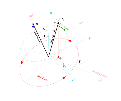
Figure 14: Inertial (fixed) coordinate system ($x,y,z$, light blue) and coordinate system moving with the orbit plane ($x^{*},y^{*},z^{*}$, red), with $z^{*}$ parallel to the orbit normal $n$ and $x^{*}$ along the ascending node. $s$ is the spin axis, the obliquity (axial tilt) $\epsilon$ is the angle between $s$ and $n$ ($\cos\mbox{$\epsilon$}=\mbox{$\mbox{\boldmath$n$}$}\cdot\mbox{$\mbox{\boldmath$s$}$}$). $\Omega$ is the longitude of the ascending node, $I$ is the orbital inclination (angle between $z^{*}$ and $z$), and $\phi$ measures the precession angle in the orbit plane (see text). $s$ slowly precesses westward (clockwise) along the ecliptic in the opposite direction (retrograde, green arrow and green dashed line) to Earth’s orbital motion (red arrows) and spin. The planetary (or ecliptic) precession is indicated by the small blue arrow (see text).

The second type of astronomical solutions discussed here (in addition to orbital solutions), are Precession-Tilt (PT) solutions. As mentioned above, precession and tilt (= obliquity) are among the most frequently used orbital parameters in the Earth sciences (see Fig. 1). Defining obliquity ($\epsilon$) is straightforward, that is, $\epsilon$ is the angle between Earth’s spin axis and the orbit normal, i.e., unit vectors $s$ and $n$, where $n$ is perpendicular to Earth’s orbital plane = ecliptic (see Fig. 14). Equivalently, obliquity is the angle between the celestial equator and the ecliptic. In contrast, the term precession may be used interchangeably in the literature for different concepts/motions. Moreover, the geometric description, as well as the different notations and symbols used by different authors, is often confusing. Importantly, however, an accurate description of precession is inevitably somewhat more complex because of the various motions and angles involved. Most critical for cyclostratigraphic and astrochronological applications is being aware of the differences between climatic and luni-solar precession, as well as nodal and apsidal precession (Section 2.1.3).

3.1 Luni-Solar and Climatic Precession

At present, the Earth rotates on its axis at an angular velocity of $\sim$7.29$\times 10^{-5}$ rad s^-1 (see spin axis vector $s$, Fig. 14). The spin axis itself slowly precesses westward (clockwise, precession angle $\phi$, Fig. 14) along the ecliptic in the opposite direction (retrograde, green arrow) to Earth’s orbital motion and spin (red arrows, see also Fig. 1). The axial precession (rate) along the fixed ecliptic with respect to space is referred to as luni-solar precession (Williams, 1994). The present precession rate of the total space motion at $t_{0}$ is $\mbox{$\Psi_{0}$}\simeq 50.38$ ^′′ y^-1 (Capitaine et al., 2003), corresponding to a period of $\sim$25.7 kyr ($\Psi$ represents a frequency, i.e., rate of change = time derivative, see Section 3.2; conventionally, $\Psi$ is taken positive). Over time, the axial precession therefore causes a notable motion of the equinoxes westward along the ecliptic. When it comes to astronomical forcing of Earth’s climate, however, it is not the position of the equinoxes relative to the fixed stars that matters ($\phi$ alone) but the position relative to Earth’s elliptic orbit (see Section 1.1), i.e., the perihelion (for further illustrations, see, e.g., Hinnov, 2018; Lourens, 2021). In addition, the forcing depends on orbital eccentricity (in a circular orbit where $e=0$, for example, the equinox position is inconsequential). Climate forcing is thus controlled by the climatic precession $\bar{p}$ (see Fig. 1):

$$\mbox{$\bar{p}$}=e\sin\mbox{$\bar{\omega}$}\ ,$$ (8)

where $\mbox{$\bar{\omega}$}=\mbox{$\varpi$}+|\mbox{$\phi$}|$ is the longitude of perihelion measured from the moving equinox (see below for $\phi$’s sign; note also that various symbols are used for $\bar{\omega}$ in the literature). As a result, precessional climate forcing does not follow a simple sine function with 25.7-kyr periodicity but depends on the frequency spectra of $\varpi$ and $\phi$, with its amplitude modulated by $e$ (see Figs. 1 and 15).

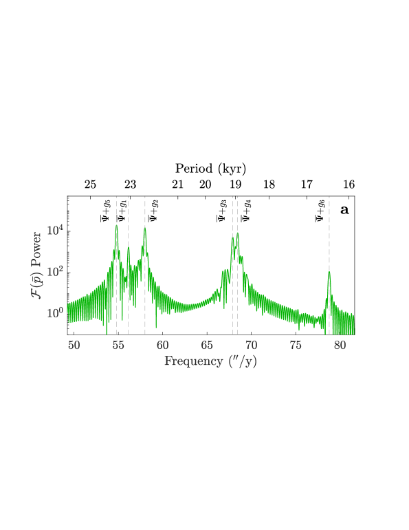
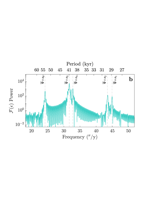
Figure 15: (a) FFT$\ =\mbox{$\cal F$}(\mbox{$\bar{p}$})$ of climatic precession ($\mbox{$\bar{p}$}=e\sin\mbox{$\bar{\omega}$}$) and (b) FFT$\ =\mbox{$\cal F$}(\mbox{$\epsilon$})$ of obliquity, both from snvec output based on ZB18a(1,1) (see Section 3.3) over a 6-Myr interval ($-6$ to 0 Myr).

Given that the precession rate is related to $\Psi$ and $\varpi$’s rate is related to the g-mode frequencies $g_{i}$ (see Section 2.1.3), one might expect that a spectral analysis of the climatic precession would show peaks at $\mbox{$\overline{\Psi}$}+g_{i}$, where $\overline{\Psi}$ is the mean $\Psi$ across the analyzed interval. For retrograde axial precession and prograde apsidal precession, the frequencies add up to a higher frequency. Indeed $\bar{p}$’s power spectrum shows dominant peaks, for instance, at $\sim$19, $\sim$22.4, and $\sim$23.7 kyr, corresponding to $\mbox{$\overline{\Psi}$}+g_{i}$ where $i=3,4,2$ and 5 (Fig. 15). Analogous to $\mbox{$\overline{\Psi}$}+g_{i}$, which yields the precession frequencies, $\mbox{$\overline{\Psi}$}+s_{i}$ yields the obliquity frequencies. Note that the dominant $g_{i}$ are positive and the dominant $s_{i}$ are negative. For retrograde axial precession and retrograde nodal precession, the frequencies combine to a lower frequency. Thus, precession and obliquity frequencies are higher and lower than the luni-solar precession rate, respectively (inversely for the periods, see Table 6 and Figs. 15 and 19).

Table 6: Frequencies (ordered by amplitude) of climatic precession ($\bar{p}$) and obliquity ($\epsilon$).^a

Frequency	Value	Period	Note
	(′′ y-1)	(kyr)
$\mbox{$\overline{\Psi}$}+g_{5}$	54.79	23.65
$\mbox{$\overline{\Psi}$}+g_{2}$	57.99	22.35
$\mbox{$\overline{\Psi}$}+g_{4}$	68.45	18.93
$\mbox{$\overline{\Psi}$}+g_{3}$	67.90	19.09
$\mbox{$\overline{\Psi}$}+g_{1}$	56.14	23.08
$\mbox{$\overline{\Psi}$}+g_{6}$	78.78	16.45
	——
$\mbox{$\overline{\Psi}$}+s_{3}$	31.69	40.90
$\mbox{$\overline{\Psi}$}+s_{4}$	32.79	39.52
$\mbox{$\overline{\Psi}$}+s_{3}+g_{43}$	32.21	40.23	b
$\mbox{$\overline{\Psi}$}+s_{6}$	24.19	53.57
$\mbox{$\overline{\Psi}$}+s_{3}-g_{43}$	31.17	41.58	b
$\mbox{$\overline{\Psi}$}+s_{1}$	44.94	28.84

^a From FFT of snvec output based on ZB18a(1,1) (see Section 3.3) over 6-Myr interval ($-6$ to 0 Myr). Note that identifying $\mbox{$\overline{\Psi}$}+s_{2}$ in $\epsilon$’s spectrum is obscured due to several large $s_{2}$ side peaks (see Fig. 5) that are unresolved over a 6-Myr interval.
^b $g_{43}=\mbox{($g_{4}$$-$$g_{3}$)}$. Note $g$-$s$ interaction (see Zeebe, 2022).

Different approaches may be used to compute PT solutions. Some methods are based on series expansions or integration of equations for the angles involved (e.g., Sharaf and Boudnikova, 1967; Berger, 1976; Kinoshita, 1975, 1977; Berger et al., 1989; Laskar et al., 1993). Other methods are based on integrating equations for Earth’s spin vector (e.g., Goldreich, 1966; Quinn et al., 1991; Touma and Wisdom, 1994; Zeebe, 2022). The latter approach allows physical insight into the torques involved (see A), provides a simple error metric for accuracy during spin vector integration, and can be applied using the most up-to-date orbital solutions (see Sections 2.5 and 3.4). Numerical routines to compute PT solutions based on Earth’s spin vector are freely available in C (snvec) and R (snvecR) at github.com/rezeebe/snvec and github.com/japhir/snvecR.

As noted above, axial precession is retrograde, that is, the equinoxes move in the opposite direction to Earth’s orbital motion and spin (see Fig. 14). Given the rule that angles measured in the orbital plane are increasing eastward (prograde or anticlockwise, see Fig. 2), it follows $\dot{\mbox{$\phi$}}_{0}<0$ (Zeebe and Lourens, 2022a; Zeebe, 2022). Note that the general precession (usually denoted as $p_{A}$, see below) is often used in this context with $\dot{p_{A}}>0$ at $t_{0}$ (e.g., Lieske et al., 1977; Williams, 1994). For appropriate initial conditions that refer to the same reference epoch (e.g., ${p_{A}}(0)=\mbox{$\phi$}(0)=0$), it follows $p_{A}=-\mbox{$\phi$}$ (see Section 3.2).

3.2 Luni-Solar (Equatorial) and Planetary (Ecliptic) Precession

As mentioned above (and pointed out before, e.g., Williams, 1994; Hilton et al., 2006), confusion may also arise over precession because of different notations and symbols. For example, luni-solar precession and planetary precession (see below) may formally be referred to as precession of the equator and precession of the ecliptic, respectively (Fukushima, 2003; Hilton et al., 2006). The two quantities are critical for understanding the link between solar system dynamics and spin axis dynamics, and hence between OS and PT solutions.

The luni-solar precession rate (here symbol $\Psi$, see Table 1) at $t_{0}$ ($\mbox{$\Psi_{0}$}>0$) may be calculated from (e.g., Ward, 1974; Quinn et al., 1991; Williams, 1994):

$$\mbox{$\Psi_{0}$}=\mbox{$\alpha$}\cos\mbox{$\epsilon$}_{0}+\mbox{$\gamma_{gp}$}\ ,$$ (9)

where $\alpha$ is often referred to as precession “constant” (A, although cf. Section 3.2.1), $\mbox{$\epsilon$}_{0}$ is the obliquity angle at $t_{0}$, and $\gamma_{gp}$ is the geodetic precession (for details, see Quinn et al., 1991; Zeebe, 2022). Eq. (9) strictly only applies at $t_{0}$ and does not capture certain periodic variations (with long-term zero averages though). Note that $\Psi$ is a rate (unit ^′′ y^-1), not an angle (the angle is usually denoted as $\Psi_{A}$, index ‘$A$’ for accumulated). $\Psi$ refers to the total precessional space motion in an inertial coordinate system (fixed ecliptic, see Williams, 1994). However, for many applications, the motion relative to the moving ecliptic may be relevant (not to be confused with the moving equinoxes, see Section 3.1). As discussed in Section 2, the planetary orbits are not stationary but move in space over time due to mutual interactions. Thus, the motion of Earth’s orbital plane (ecliptic) contributes to the precessional motion (planetary or ecliptic precession, see Fig. 14, small blue arrow). The precession relative to the moving ecliptic is referred to as general precession in longitude ($\mbox{$p_{A}$}=-\mbox{$\phi$}$, see Fig. 14), or just general precession. Note that $p_{A}$ is an angle; its rate is $d\mbox{$p_{A}$}/dt=\dot{p}_{A}$. In summary, with respect to $\phi$, we may write:

$$\phi=-p_{A}\qquad;\qquad\dot{\mbox{$\phi$}}=-\dot{p}_{A}\ .$$ (10)

Briefly, the important difference between $\phi$ and $\dot{\mbox{$\phi$}}$ vs. $\Psi$ and $\dot{\Psi}$ is that the first two are measured in the moving ecliptic frame, while the last two are measured in the inertial frame.

Figure 16: (a) Precession angle $\phi$ (in moving ecliptic frame, see Fig. 14) and $-\mbox{$\Psi$}_{A}$ (in inertial frame); both angles are taken as zero at $t_{0}$. (b) Time derivative of precession angle $|\dot{\mbox{$\phi$}}|$ (in moving ecliptic frame) and luni-solar precession $\Psi$ (in inertial frame). $\Psi$ is conventionally taken positive. Note that $\Psi$ is not constant over time and the difference $|\dot{\mbox{$\phi$}}|-\mbox{$\Psi$}$ (ecliptic motion) is small at $t_{0}$, but not in general.

Once $\dot{p}_{A}$ and $\Psi$ and have been calculated, the precession components are often separated into a luni-solar and planetary contribution. At $t_{0}$, the difference $\dot{p}_{A}-\mbox{$\Psi$}$ (ecliptic motion) may be written as (Williams, 1994):

$$\dot{p}_{A,0}-\mbox{$\Psi_{0}$} = 50.2880-50.3848=-0.0968\qquad\mbox{[\mbox{${}^{\prime\prime}${\,}y\mbox{${}^{-1}$}}]}\ ,$$ (11)

where Capitaine et al. (2003)’s values have been used (see Table 1). Similar values have been obtained based on a variety of approaches (e.g., Lieske et al., 1977; Laskar et al., 1993; Williams, 1994; Simon et al., 1994; Roosbeek and Dehant, 1998; Capitaine et al., 2003; Fukushima, 2003; Hilton et al., 2006; Vondrák et al., 2011). From Eq. (11) it may appear that the ecliptic motion is much smaller than the general motion. However, Eq. (11) only applies to the ecliptic vs. general motion at $t_{0}$ and not generally at all times (see Fig. 16 and Vondrák et al. (2011)).

For certain paleo-applications such as deep-time studies, the details and differences between the various precessional quantities discussed above may not matter because the long-term means of, e.g., $\Psi$, $|\dot{\mbox{$\phi$}}|$, and Eq. (9) are very similar. However, it is clear that $\Psi$, for instance, is not constant over time but varies periodically on Milanković time scales and exhibits long-term secular trends (Figs. 16 and 19). Moreover, its precise value depends on the precessional model employed and the dynamical ellipticity value at $t_{0}$ (see Section 3.3). Thus, providing precessional parameters or $\Psi_{0}$ with a large number of digits appears unnecessary for practical applications (except for check values in numerical routines).

3.2.1 Luni-Solar Precession: Long-term Variations

Considering only short-term variations in $\Psi$ (see Eq. (9)), the parameter $\alpha$ may be indeed be taken as constant (see A). However, considering long-term variations in $\Psi$, $\alpha$ is far from constant due to the long-term evolution of the Earth-Moon system, including changes in Earth’s rotation, lunar distance, tidal dissipation, dynamical ellipticity, etc. (see Section 3.5). For instance, ignoring the small term $\gamma_{gp}$ and setting $\mbox{$\kappa$}=g_{L}=1$ (see A), Eq. (9) may be re-written as:

$$\Psi = {\cal C}\ \frac{H}{\mbox{$\Omega_{E}$}}\left(1+\frac{a^{3}}{a_{L}^{3}}\frac{m_{L}}{M_{S}}\right)\ \cos\mbox{$\epsilon$}\ ,$$ (12)

where ${\cal C}=\frac{3}{2}\frac{GM}{a^{3}}$, $H$ is the dynamical ellipticity (see Section 3.3), $\Omega_{E}$ is Earth’s angular speed, $a$ the semi-major axis of its orbit, $a_{L}$ the Earth-Moon distance parameter, and $m_{L}/M_{S}$ the lunar to solar mass ratio. Furthermore, $H\propto\ \mbox{$\Omega$}_{E}^{2}$ (see Section 3.3) and hence:

$$\Psi = {\cal D}\ \mbox{$\Omega_{E}$}\left(1+\frac{a^{3}}{a_{L}^{3}}\frac{m_{L}}{M_{S}}\right)\ \cos\mbox{$\epsilon$}\ ,$$ (13)

where ${\cal D}$ may be taken as constant (to first order) over long time scales. Eq. (13) illustrates the large secular decrease in $\Psi$ over geologic time (i.e, increase in period, see Fig. 19) due to the slow-down of Earth’s rotation ($\Omega_{E}$) and the simultaneous increase in lunar distance ($a_{L}$). The two processes are coupled via conservation of angular momentum (e.g., Goldreich, 1966; Touma and Wisdom, 1994; Farhat et al., 2022; Zeebe and Lantink, 2024b; Malinverno and Meyers, 2024). Finally, note that several recent studies have estimated long-term variations in luni-solar precession frequency from stratigraphic data (see, e.g., Wu et al., 2024, and references therein).

3.3 Dynamical Ellipticity and Tidal Dissipation

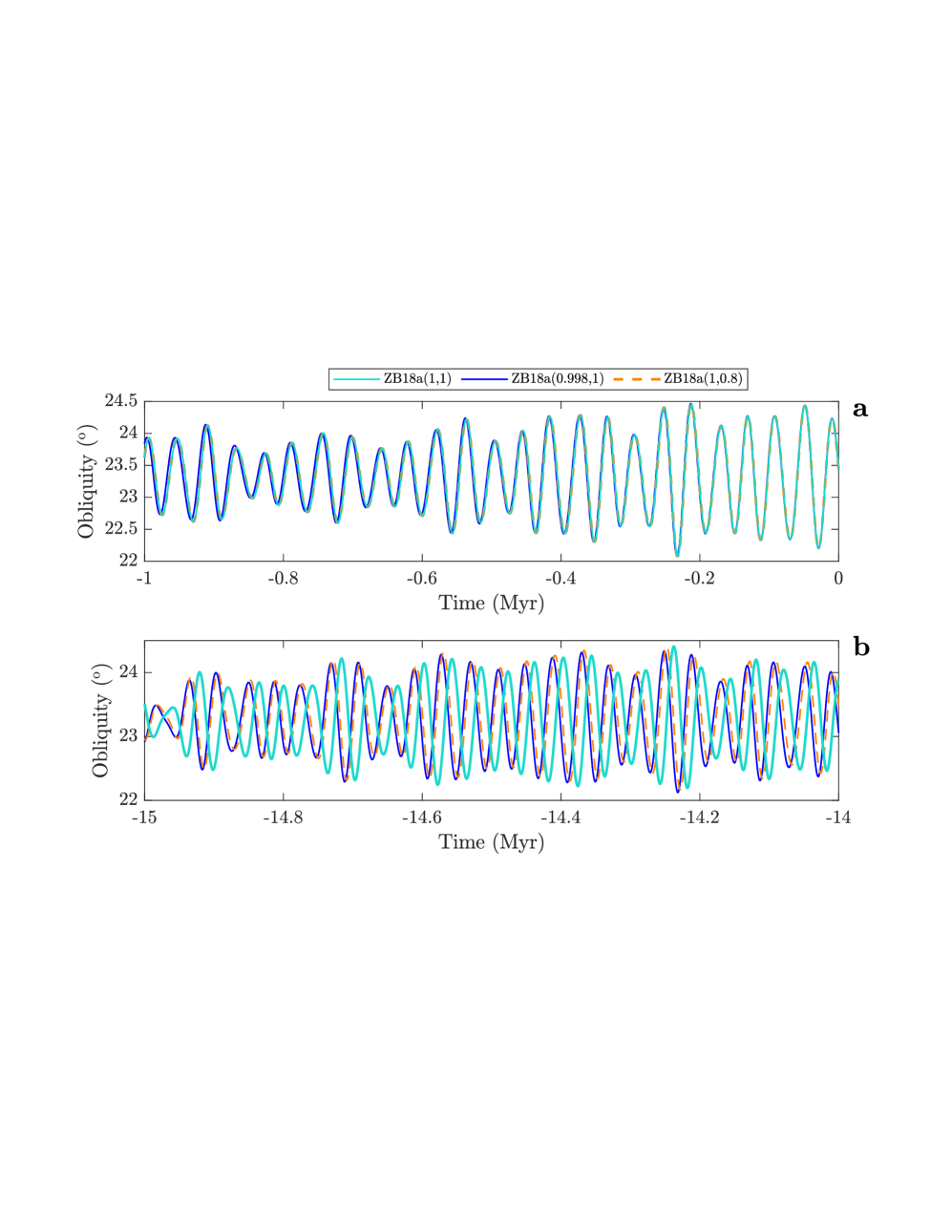
Figure 17: Illustration of changes in Earth’s dynamical ellipticity ($E_{d}$) and tidal dissipation ($T_{d}$) affecting the numerical solution for Earth’s obliquity over 15 Myr (for details on the numerical parameters $E_{d}$ and $T_{d}$, see Zeebe and Lourens, 2022a). In runs labeled $\mbox{$E_{d}$}=0.998$ and $\mbox{$T_{d}$}=0.8$, the values of $E_{d}$ and $T_{d}$ were set to 99.8% and 80%, respectively, of their modern values $\mbox{$E_{d}$}=\mbox{$T_{d}$}=1.0$. (a) $-1$ to 0 Myr, the solutions are nearly identical. (b) $-14$ to $-15$ Myr, the solutions are out of phase, which would cause significant dating errors.

Dynamical ellipticity refers to the gravitational shape of the Earth, largely controlled by the hydrostatic response to its rotation rate. Dynamical ellipticity is defined as $H=[C-(A+B)/2]/C$, where $C$ is the polar moment of inertia and $A$ and $B$ are the equatorial moments of inertia. If $A=B$,

$$H=(C-A)/C\qquad;\qquad H\propto\ \mbox{$\Omega$}_{E}^{2}\ .$$ (14)

Importantly, $H$’s hydrostatic response is proportional to $\mbox{$\Omega$}_{E}^{2}$, where $\Omega_{E}$ is Earth’s spin, or angular velocity (Lambeck, 1980). The present value of $H$ is $\sim$0.00328; however, its precise, absolute value is usually adjusted to other parameters and hence may differ between models (e.g., Quinn et al., 1991; Laskar et al., 1993; Williams, 1994; Capitaine et al., 2003; Chen et al., 2015; Zeebe, 2022). Note that the calculated changes in obliquity and precession in the past are sensitive to even small changes in dynamical ellipticity (see Fig. 17), which is affected by, e.g., $\Omega_{E}$, ice volume, and mantle convection (e.g., Berger et al., 1989; Laskar et al., 1993; Morrow et al., 2012; Zeebe and Lourens, 2022a). Regarding the effect of Earth’s dynamical ellipticity and Earth’s rotation rate on the luni-solar precession rate (see Eq. (9)), it is important that the precession constant $\alpha$ is proportional to $H$ and inversely proportional to $\Omega_{E}$ (see A). Thus, because $H\ \propto\ \mbox{$\Omega_{E}$}^{2}$,

$$\mbox{$\alpha$}\ \propto\ \mbox{$\Omega_{E}$}\ .$$ (15)

Tidal dissipation refers to the energy dissipation in the earth and ocean, which reduces Earth’s rotation rate and increases the length of day and the Earth-Moon distance. The parameter relevant here for PT solutions is the change in lunar mean motion $n_{L}$ (average angular frequency), which is presently decreasing at a rate:

$$Q_{0}=(dn_{L}/dt)_{0}/(n_{L})_{0}=-4.6\mbox{$\times 10^{-18}$}\ \mbox{s\mbox{${}^{-1}$}}$$ (16)

(Quinn et al., 1991). Reconstructing $T_{d}$’s history involves considerable uncertainties and remains an active area of research, specifically the development of model frameworks for the Earth-Moon’s tidal evolution focusing on the long-term history of ocean tidal dissipation (e.g., Webb, 1982; Hansen, 1982; Kagan and Maslova, 1994; Green et al., 2017; Motoyama et al., 2020; Daher et al., 2021; Tyler, 2021; Farhat et al., 2022; Zeebe and Lantink, 2024b).

The combined precession-tilt-orbital solution may be denoted as OS($E_{d}$,$T_{d}$), see Zeebe and Lourens (2022a). For example, ZB18a(1,1) refers to a PT solution based on the orbital solution ZB18a with modern values $\mbox{$E_{d}$}=1$ and $\mbox{$T_{d}$}=1$ (see Figs. 15 and 17). Relatively simple parameterizations using $E_{d}$ and $T_{d}$ as employed in Zeebe and Lourens (2022a) are most useful over, say, the Cenozoic, where changes in $\Psi$, Earth-Moon distance, etc. are comparatively small (Quinn et al., 1991; Zeebe and Lourens, 2022a; Zeebe, 2022). In order to compute full PT solutions in deep time, say, on Gyr-time scale, a fundamentally different approach is required that considers the long-term evolution of the Earth-Moon system, as well as the large scale dynamical chaos in the solar system (see Sections 3.2.1, 3.5 and Zeebe and Lantink, 2024a, b).

3.4 Up-to-date Precession and Obliquity Solutions

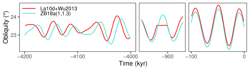
Figure 18: Obliquity solution based on the procedure by Wu et al. (2013) for La10x currently available in the Acycle package (Li et al., 2019) (example: La10d+Wu2013, red). For comparison, obliquity calculated using snvec (Zeebe and Lourens, 2022b) based on ZB18a (Zeebe and Lourens, 2019) (ZB18a(1,1.3), turquoise, see text for details).

Wu et al. (2013) suggested and employed a procedure to obtain obliquity and precession solutions using the orbital solutions La10x from Laskar et al. (2011) and the Fortran code from Laskar et al. (1993) (for an example following Wu et al. available in the Acycle package (Li et al., 2019), see Fig. 18). Wu et al. (2013) used the parameter values $\texttt{FGAM}=1.0$ and $\texttt{CMAR}=1.3$. Importantly, the Wu et al. (2013) procedure/output has also been used in subsequent studies (e.g., Laurin et al., 2015; Ma et al., 2017, 2019). However, the La10x output is incompatible with the 1993-Fortran routine because of different reference frames (see below). Here we illustrate the problematic obliquity solution by comparison with Zeebe and Lourens (2019), from which we calculate obliquity using snvec (Zeebe and Lourens, 2022b) and the values for $E_{d}=1$ and $T_{d}=1.3$. The Acycle output is offset already at $t=0$ (see Fig. 18). Furthermore, at around $-900$ kyr, part of the cycle is clipped, which appears to be a numerical error. At around $-4$ Myr the Wu et al. (2013) solution is offset from Zeebe and Lourens (2022b) by about half a cycle.

The problem with the approach of Wu et al. (2013) is incompatible reference frames (see Section 2.1.2). The 1993-Fortran routines from Laskar et al. (1993) expect orbital elements given in the ecliptic reference frame. However, the La10x elements are given in the invariant reference frame (Laskar et al., 2011). As explained above, the invariant frame is based on the invariable plane (perpendicular to the solar system’s total angular momentum vector that passes through its barycentre) and is hence different from the ecliptic frame. Wu et al.’s procedure is therefore not recommended. For the user interested in PT solutions based on up-to-date orbital solutions, say, for the Cenozoic, the freely available routines snvec and snvecR are recommended (github.com/rezeebe/snvec and github.com/japhir/snvecR). These routines can be used with up-to-date orbital solutions such as ZB18a and ZB20x that supply orbital elements in a compatible reference frame. For the application-oriented user, pre-computed and up-to-date PT solutions for different $E_{d}$ and $T_{d}$ values are readily available for download (no programs, coding, etc. involved), see www.ncdc.noaa.gov/paleo/study/35174 (Zeebe and Lourens, 2022a). PT solutions here refer to full solutions (including individual PT cycles and temporal resolution of order $10^{2}$-$10^{3}$ y), rather than calculated frequencies and long-term averages.

3.5 Milanković Forcing in Deep Time

This review has largely focused on the past few 100 Myr. Milanković forcing for older intervals (deep time) needs to consider a host of additional factors, including tidal dissipation, the long-term evolution of the Earth-Moon system, solar mass loss, and more. Unfortunately, a comprehensive review of astronomical forcing in deep time is beyond the scope of this paper. Instead, we refer the reader to recent work specifically dedicated to Milanković forcing in deep time (Zeebe and Lantink, 2024a, b), as well as related studies (e.g., MacDonald, 1964; Goldreich, 1966; Mignard, 1981; Berger et al., 1989; Ito et al., 1993; Touma and Wisdom, 1994; Ito et al., 1995; Waltham, 2015; Meyers and Malinverno, 2018; Spalding et al., 2018; Farhat et al., 2022; De Vleeschouwer et al., 2024; Malinverno and Meyers, 2024). The evolution of the main periods of eccentricity, tilt, and precession (ETP) on Gyr-time scale may be summarized in a nutshell as follows (see Fig. 19). The average precession and obliquity periods ($\mbox{$\overline{\Psi}$}+g_{i}$ and $\mbox{$\overline{\Psi}$}+s_{i}$) increase with time due to the changing luni-solar precession $\overline{\Psi}$ (averaged over 20 Myr intervals), accompanied by the slowing of Earth’s rotation, lengthening of the day, and the receding Moon. The short eccentricity periods ($\sim$95, 99, 124, and 131 kyr recent) appear relatively stable but actually exhibit substantial variations in frequency and amplitude and do not serve as metronomes (Zeebe and Lantink, 2024b). The spikes in the long eccentricity cycle ($g_{2}$$-$$g_{5}$) (top, Fig. 19) reflect instabilities in $g_{2}$, which compromises the 405-kyr cycle’s reliability beyond several hundred million years in the past, as mentioned above (Zeebe and Lantink, 2024a). One major issue identified by Zeebe and Lantink (2024a) is that the long eccentricity cycle may not be available as a primary tuning target in deep time.

Importantly, the direct use of astronomical solutions for astronomical tuning (e.g., for absolute ages and chronologies across the Cenozoic) represents only one realm of the use of astronomical solutions in astrochronology. As pointed out in Section 1, much of the ongoing astrochronological work on the geologic time scale uses relative (floating) age models, spanning most of Earth’s history, that is, the entire pre-Cenozoic. Pre-Cenozoic studies also rely on astronomical solutions in a range of capacities, even when explicit cycle-to-cycle tuning in the time domain is not possible due to uncertainties in amplitude, phase, and frequency of the forcing due to chaos and uncertainties in parameters such as tidal dissipation, dynamical ellipticity, etc. For more information on pre-Cenozoic astronomical parameters, we refer the reader to recent theoretical work (e.g., Spalding et al., 2018; Daher et al., 2021; Tyler, 2021; Farhat et al., 2022; Zeebe and Lantink, 2024a, b), as well as observational work using the geologic record (e.g., Zhang et al., 2015; Ma et al., 2017; Meyers and Malinverno, 2018; Kent et al., 2018; Lantink et al., 2019; Olsen et al., 2019; Sørensen et al., 2020; Lantink et al., 2022, 2023, 2024; Malinverno and Meyers, 2024; Wu et al., 2024).

This section concludes our review of orbital solutions and precession-tilt solutions. The remaining sections deal with practical considerations, summary, and outlook.

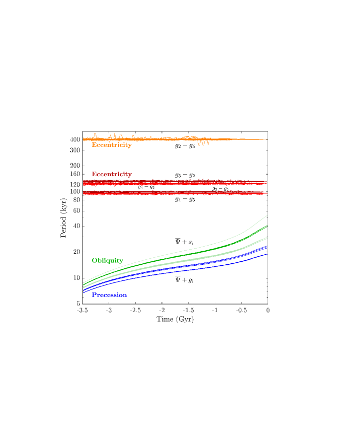
Figure 19: Summary of eccentricity, tilt, and precession (ETP) periods from 3.5-Gyr integrations (Zeebe and Lantink, 2024a, b). Note the logarithmic ordinate. $\overline{\Psi}$ refers to the averaged luni-solar precession over 20 Myr intervals.

4 Practical Considerations

In the following, we provide a few recommendations and list selected resources for practical consideration. First, regarding orbital solutions, the user needs to consider their valid time span, which is limited fundamentally by solar system chaos (see Table 5). As pointed out above, the probability that a particular OS represents the actual, unique history of the solar system is near zero significantly beyond the OS’s validity range. For example, finding a good match between, say an eccentricity record at 100 Ma and La04 would be entirely coincidental and concluding that La04 is therefore a proper solution of the solar system orbits over the past 100 Myr would be misleading (see Section 2.5). Instead, for the time being, we recommend the solutions ZB18a and ZB20x across the time span from $-300$ to 0 Myr, available at www.ncdc.noaa.gov/paleo/study/36415 and www2.hawaii.edu/~zeebe/Astro.html. Note though that these solutions have been constrained by geologic data only up to an age of 66 Ma (Table 5). Beyond $-300$ Myr, the ZB23x solutions may serve as possible templates for deep time characteristics (see www.ncdc.noaa.gov/paleo/study/39199). Importantly, however, no single solution should be considered the “true” solution.

For up-to-date precession-tilt solutions, we recommend choosing between two options at this time (see Section 3.4). One option is downloading pre-calculated PT solutions for different values of $E_{d}$ and $T_{d}$, available at www.ncdc.noaa.gov/paleo/study/35174 and www2.hawaii.edu/~zeebe/Astro.html (see Zeebe and Lourens, 2022a; Zeebe, 2022). Another option is for the user to generate their own PT solutions based on up-to-date orbital solutions using our snvec code in C or R available at github.com/rezeebe/snvec and github.com/japhir/snvecR (for summary, see Table 7). We do not recommend the procedure proposed by Wu et al. (2013) to generate PT solutions (see Section 3.4). For the user interested in generating insolation curves based on up-to-date orbital solutions, we mention here a web-based user interface currently under construction at astrocyclo.soest.hawaii.edu.

4.1 Available Resources

To assist the user in identifying available resources for the analysis of their specific problem at hand, we list a few selected solutions, codes, and tools (including URLs, see Table 7). The list is far from exhaustive and focuses on resources that are up-to-date (including OS/PT solutions), open source, directly accessible, frequently used, and maintained. Assume the user’s goal is, for example, to develop a cyclostratigraphic age model for a Miocene record based on astronomical tuning to Earth’s precession and obliquity. For the time series analysis of the data record, tools such as astrochron and Acycle are available (Table 7). For the astronomical tuning to precession and obliquity, PT solutions based on ZB18a with different values for $E_{d}$ and $T_{d}$ are available for download at www2.hawaii.edu/~zeebe/Astro.html (Zeebe and Lourens, 2022a; Zeebe, 2022). Given a task/time interval at hand and the information compiled in Tables 5 and 7, most users seeking guidance should be able to identify resources for the analysis of their problem using astronomical solutions and Milanković forcing as reviewed in the present paper. The experienced user is of course free to employ the tools of their choice. However, regarding astronomical solutions, we strongly recommend considering the recency, limitations, and valid time span of the solutions (see Sections 2.5 and 3.4). Tools that yield inaccurate results should be abandoned (see Section 3.4).

Table 7: Selected resources (up-to-date OS/PT solutions, open source, directly accessible, frequently used, maintained).

Resource Type	Name/ID	Reference	URL
Orbital Solution	ZB23x	Zeebe and Lantink (2024a)	a,b
Orbital Solution	ZB18a ZB20x	Zeebe and Lourens (2019, 2022b)	c,a
Orbital Solution	La10x	Laskar et al. (2011)	d
PT Solution	ZB18a($E_{d}$,$T_{d}$)	Zeebe and Lourens (2022a); Zeebe (2022)	e,a
Insolation web-interface	astrocyclo	under construction	f
Orbit Integrator+Code (C)	orbitN	Zeebe (2023)	g,a
PT Integrator+Code (C, R)	snvec snvecR	Zeebe (2022)	h,a
Integrator+Code (C, Python)	rebound	Rein and Liu (2012)	i
Astrochronology Tool (R)	astrochron	Meyers (2014)	j
Time Series Analysis Tool	Acycle	Li et al. (2019)	k

^a www2.hawaii.edu/~zeebe/Astro.html
^b www.ncdc.noaa.gov/paleo/study/39199
^c www.ncdc.noaa.gov/paleo/study/26970 $|$ www.ncdc.noaa.gov/paleo/study/36415
^d vo.imcce.fr/insola/earth/online/earth/La2010/index.html
^e www.ncdc.noaa.gov/paleo/study/35174
^f astrocyclo.soest.hawaii.edu
^g github.com/rezeebe/orbitN
^h github.com/rezeebe/snvec $|$ github.com/japhir/snvecR
ⁱ rebound.readthedocs.io/en/latest
^j cran.r-project.org/web/packages/astrochron/index.html
^k acycle.org

5 Summary & Outlook

We have reviewed astronomical solutions and Milanković forcing as applied in the Earth sciences. Given confusion and recent inaccurate results in the application of astronomical solutions, our review appears appropriate and timely, and clarifies the astronomical basis, applicability, and limitations of astronomical solutions. Applying accurate and up-to-date solutions and tools is critical to extend and improve the astronomical time scale, which, over the past few decades, has transformed the dating of geologic archives. Today, astronomical solutions and the astronomical time scale represent the backbone of astrochronology and cyclostratigraphy, widely used in the Earth sciences. In our review, we have discussed two fundamental types of astronomical solutions and their limitations: orbital solutions (OSs) and precession-tilt (PT) solutions. While OSs are a prerequisite and essential for PT solutions, the reverse effects of rotational dynamics on OSs are generally minor.

To understand the behavior of orbital solutions and astronomical forcing terms, we have emphasized the analysis of the fundamental (secular) frequencies, which may be thought of as the spectral building blocks of the dynamical system. The secular frequency analysis also provides insight into amplitude and frequency modulation of orbital forcing signals and leads to the conclusion that the current evidence does not support the notion of generally stable and prominent astronomical “metronomes” for universal use in astrochronology and cyclostratigraphy. Large-scale dynamical chaos is an inherent characteristic of the solar system and fundamental to understanding the behavior of astronomical solutions and their limitations. We have illustrated the unpredictability and unaccountability of chaotic systems in terms of basic statistics. One important corollary is that it is generally not possible to “tune” or “fit” astronomical solutions to geological data. The best that can probably be done is to create large ensembles of solutions via parameter variations and select/discard those solutions that show good/poor agreement with the data. Our in-depth description of the various quantities associated with Earth’s axial precession should aid in clarifying the terminology and notation appearing in the literature. We have also discussed astronomical forcing and astrochronology in deep time, which represents another critical application of astronomical solutions beyond the direct use for astronomical tuning of, say, absolute Cenozoic ages and chronologies. Finally, our summary of selected available resources should assist the interested user in identifying resources for the analysis of their specific problem at hand, using the astronomical solutions and Milanković forcing as reviewed here.

Continuing improvements in computer technology, speed, and algorithms will accelerate numerical computations in the future and will allow integrating more complete and complex models of the solar system (for recent endeavors, see, e.g., Brown and Rein, 2020; Zeebe, 2023; Javaheri et al., 2023; Hernandez and Dehnen, 2024). Importantly, however, the limits imposed by dynamical chaos on astronomical calculations and geological/astrochronological applications are fundamental and physical in nature, and cannot be overcome by numerical advances. In order to generate ensemble solutions with long (and specific) divergence times, arbitrary precision code might be helpful. One goal regarding user access to up-to-date astronomical solutions in the future is offering more user-friendly applications, such as a web-based user interface (for current efforts in progress/under construction, see, e.g., astrocyclo.soest.hawaii.edu). In terms of future observational endeavors, it is highly desirable to obtain high-quality cyclostratigraphic sequences that constrain the evolution of Earth’s precession and obliquity frequencies across the Cenozoic, as well as in deep time, the latter being critical to reconstructing the Earth-Moon system’s long-term evolution. (see, e.g., Wu et al., 2024, and references therein). New high-quality eccentricity and obliquity records older than $\sim$50 Ma will be crucial in constraining the solar system’s chaotic history, and in turn, in providing highly accurate geological dates and chronologies for cyclostratigraphy and astrochronology.

Acknowledgments. We thank one anonymous reviewer, Dorian Abbot, Alberto Malinverno, and Steve Meyers for their thorough reviews, which improved the paper. We are grateful to Alberto Malinverno and Steve Meyers for specific text suggestions that refined and extended the manuscript content. We also thank David M. Hernandez and Margriet Lantink for helpful comments on the manuscript draft. This research was supported by Heising-Simons Foundation Grant #2021-2800 and U.S. NSF grant OCE20-34660 to R.E.Z.

software orbitN, github.com/rezeebe/orbitN, snvec, github.com/rezeebe/snvec, snvecR, github.com/japhir/snvecR

Appendix A Precession Equations

The calculation of precession and obliquity using our snvec code is detailed in Zeebe (2022) and Zeebe and Lantink (2024b). A few equations for the precession constant are included here for clarity (see Section 3). The change in the spin axis (unit vector $s$) is calculated from (e.g., Goldreich, 1966; Ward, 1974, 1979; Bills, 1990; Quinn et al., 1991):

$$\dot{\mbox{$\mbox{\boldmath$s$}$}}=\mbox{$\alpha$}(\mbox{$\mbox{\boldmath$n$}$}\cdot\mbox{$\mbox{\boldmath$n$}$})(\mbox{$\mbox{\boldmath$s$}$}\times\mbox{$\mbox{\boldmath$n$}$})\ ,$$ (17)

where $\alpha$ is the precession constant (although cf. Section 3.2.1) and $n$ the orbit normal (unit vector normal to the orbit plane). The obliquity (polar) angle, $\epsilon$, is given by:

$$\cos\mbox{$\epsilon$}=\mbox{$\mbox{\boldmath$n$}$}\cdot\mbox{$\mbox{\boldmath$s$}$}\ .$$ (18)

The precession (azimuthal) angle, $\phi$, measures the motion of $s$ in the orbit plane. The precession constant $\alpha$ is calculated from (e.g., Quinn et al., 1991):

$$\mbox{$\alpha$}=K\ (\mbox{$\kappa$}+\mbox{$\beta$})\ ,$$ (19)

where $\mbox{$\kappa$}=(1-e^{2})^{-3/2}$ and $e$ is the orbital eccentricity. $K$ and $\beta$ relate to the torque due to the Sun and Moon, respectively:

$$K = \frac{3}{2}\frac{C-A}{C}\frac{1}{\mbox{$\Omega_{E}$}\ a^{3}}GM_{S}$$ (20)

$$\beta = g_{L}\ \frac{a^{3}}{a_{L}^{3}}\frac{m_{L}}{M_{S}}\ ,$$ (21)

where $A$ and $C$ are the planet’s equatorial and polar moments of inertia, $(C-A)/C=H$ is the dynamical ellipticity, $\Omega_{E}$ is Earth’s angular speed, $a$ the semi-major axis of its orbit, $a_{L}$ is the Earth-Moon distance parameter, and $GM$ is the gravitational parameter of the Sun (see Table 1). The index ‘$L$’ refers to lunar properties, where $g_{L}$ is a correction factor related to the lunar orbit (Kinoshita, 1975, 1977; Quinn et al., 1991) and $m_{L}/M_{S}$ is the lunar to solar mass ratio. The parameter values used for Earth are given in Table 1 and in Zeebe (2022). With $K$ and $\beta$, $\alpha$ and hence the luni-solar precession rate $\Psi$ can be calculated (see Eq. (9)).

References

- Abbot et al. (2023) Abbot, D.S., Hernandez, D.M., Hadden, S., Webber, R.J., Afentakis, G.P., Weare, J., 2023. Simple Physics and Integrators Accurately Reproduce Mercury Instability Statistics. Astrophys. J. 944, 190. doi:10.3847/1538-4357/acb6ff, arXiv:2212.14844.
- Antoñana et al. (2022) Antoñana, M., Alberdi, E., Makazaga, J., Murua, A., 2022. An implicit symplectic solver for high-precision long-term integrations of the Solar System. Celest. Mechan. Dynamic. Astron. 134, 31. doi:10.1007/s10569-022-10081-9.
- Applegate et al. (1985) Applegate, J.H., Douglas, M.R., Gürsel, Y., Hunter, P., Seitz, C.L., Sussman, G.J., 1985. A Digital Orrery. IEEE Trans. Comput. 34, 822–831. doi:10.1109/TC.1985.1676638.
- Arnol’d (1963) Arnol’d, V.I., 1963. Proof of a Theorem of A. N. KOLMOGOROV on the Invariance of Quasi-Periodic Motions Under Small Perturbations of the Hamiltonian. Russ. Math. Surv. 18, 9–36. doi:10.1070/RM1963v018n05ABEH004130.
- Aubry et al. (2009) Aubry, M., Van Couvering, J., Christie-Blick, N., Landing, E., Pratt, B., Owen, D., Ferrusquía-Villafranca, I., 2009. Terminology of geological time: Establishment of a community standard. Stratigraphy 6, 100–105.
- Bate et al. (1971) Bate, R.R., Mueller, D.D., White, J.E., 1971. Fundamentals of Astrodynamics. Dover, New York.
- Batygin and Laughlin (2008) Batygin, K., Laughlin, G., 2008. On the dynamical stability of the solar system. Astrophys. J. 683, 1207–1216. doi:10.1086/589232.
- Berger (1977) Berger, A., 1977. Long-Term Variations of the Earth’s Orbital Elements. Celestial Mechanics 15, 53–74. doi:10.1007/BF01229048.
- Berger (1978) Berger, A., 1978. Long-term variations of daily insolation and Quaternary climatic changes. J. Atmos. Sci. 35, 2362–2367.
- Berger and Loutre (1992) Berger, A., Loutre, M.F., 1992. Astronomical solutions for paleoclimate studies over the last 3 million years. Earth Planet. Sci. Lett. 111, 369–382. doi:10.1016/0012-821X(92)90190-7.
- Berger and Loutre (1994) Berger, A., Loutre, M.F., 1994. Precession, eccentricity, obliquity, insolation and paleoclimates, in: J.-C. Duplessy and M.-T. Spyridakis (Ed.), Long-term Climatic Variations, Springer Berlin Heidelberg. pp. 107–151. doi:10.1007/978-3-642-79066-9\_5.
- Berger et al. (1989) Berger, A., Loutre, M.F., Dehant, V., 1989. Influence of the changing lunar orbit on the astronomical frequencies of pre-Quaternary insolation patterns. Paleoceanogr. 4, 555–564. doi:10.1029/PA004i005p00555.
- Berger (1976) Berger, A.L., 1976. Obliquity and precession for the last 5000000 years. Astron. Astrophys. 51, 127–135.
- Bills (1990) Bills, B.G., 1990. The rigid body obliquity history of Mars. J. Geophys. Res. 95, 14137–14153. doi:10.1029/JB095iB09p14137.
- Bretagnon (1974) Bretagnon, P., 1974. Long-period terms in the solar system. (in French) Astron. Astrophys. 30, 141–154.
- Broecker (1966) Broecker, W.S., 1966. Absolute Dating and the Astronomical Theory of Glaciation: Changes in climate occur in response to periodic variations in the earth’s tilt and precession. Science 151, 299–304.
- Broecker (1985) Broecker, W.S., 1985. How to Build a Habitable Planet. pp. 291. Eldigio Press, Lamont-Doherty Geological Observatory, Palisades, New York.
- Brouwer and van Woerkom (1950) Brouwer, D., van Woerkom, A.J.J., 1950. The secular variations of the orbital elements of the principal planets. Astronomical Papers Prepared for the Use of the American Ephemeris and Nautical Almanac 13, 81–107.
- Brown and Rein (2020) Brown, G., Rein, H., 2020. A Repository of Vanilla Long-term Integrations of the Solar System. Res. Notes American Astron. Soc. 4, 221. doi:10.3847/2515-5172/abd103, arXiv:2012.05177.
- Capitaine et al. (2003) Capitaine, N., Wallace, P.T., Chapront, J., 2003. Expressions for IAU 2000 precession quantities. Astron. Astrophys. 412, 567–586. doi:10.1051/0004-6361:20031539.
- Charbonnier et al. (2023) Charbonnier, G., Boulila, S., Spangenberg, J.E., Vermeulen, J., Galbrun, B., 2023. Astrochronology of the Aptian stage and evidence for the chaotic orbital motion of Mercury. Earth Planet. Sci. Lett. 610, 118104. doi:10.1016/j.epsl.2023.118104.
- Chen et al. (2015) Chen, W., Li, J.C., Ray, J., Shen, W.B., Huang, C.L., 2015. Consistent estimates of the dynamic figure parameters of the earth. J. Geodesy 89, 179–188. doi:10.1007/s00190-014-0768-y.
- Chirikov (1979) Chirikov, B.V., 1979. A universal instability of many-dimensional oscillator systems. Phys. Rep. (Rev. Sec. Phys. Lett.) 52, 263–379. doi:10.1016/0370-1573(79)90023-1.
- Cvijanovic et al. (2020) Cvijanovic, I., Lukovic, J., Begg, J.D., 2020. One hundred years of Milanković cycles. Nat. Geosci. 13, 524–525. doi:10.1038/s41561-020-0621-2.
- Daher et al. (2021) Daher, H., Arbic, B.K., Williams, J.G., Ansong, J.K., Boggs, D.H., Müller, M., Schindelegger, M., Austermann, J., Cornuelle, B.D., Crawford, E.B., Fringer, O.B., Lau, H.C.P., Lock, S.J., Maloof, A.C., Menemenlis, D., Mitrovica, J.X., Green, J.A.M., Huber, M., 2021. Long-Term Earth-Moon Evolution With High-Level Orbit and Ocean Tide Models. J. Geophys. Res. (Planets) 126, e06875. doi:10.1029/2021JE006875.
- Danby (1988) Danby, J.M.A., 1988. Fundamentals of celestial mechanics. Willmann-Bell Inc., Richmond, VA.
- De Vleeschouwer et al. (2024) De Vleeschouwer, D., Percival, L.M., Wichern, N.M., Batenburg, S.J., 2024. Pre-Cenozoic cyclostratigraphy and palaeoclimate responses to astronomical forcing. Nature Rev. Earth Env. 5, 59–74.
- Duriez (1977) Duriez, L., 1977. Théorie Générale Planétaire en Variables Elliptiques. I. Développement des Équation. (in French) Astron. Astrophys. 54, 93–112.
- Dutkiewicz et al. (2024) Dutkiewicz, A., Boulila, S., Müller, R.D., 2024. Deep-sea hiatus record levels orbital pacing by 2.4 Mar eccentricity grand cycles. Nature Comm. 15. doi:10.1038/s41467-024-46171-5.
- Einstein (1916) Einstein, A., 1916. Die Grundlage der allgemeinen Relativitätstheorie. Annalen der Physik, VI. Folge 49(7), 769–822. doi:10.1002/andp.19163540702.
- Emiliani (1955) Emiliani, C., 1955. Pleistocene temperatures. J. Geol. 63, 538–578.
- Emiliani (1995) Emiliani, C., 1995. Two revolutions in the Earth Sciences. Terra Nova 7, 587–597. doi:10.1111/j.1365-3121.1995.tb00706.x.
- Farhat et al. (2022) Farhat, M., Auclair-Desrotour, P., Boué, G., Laskar, J., 2022. The resonant tidal evolution of the Earth-Moon distance. Astron. Astrophys. 665, L1. doi:10.1051/0004-6361/202243445, arXiv:2207.00438.
- Fränz and Harper (2002) Fränz, M., Harper, D., 2002. Heliospheric coordinate systems. Planet. Space Sci. 50, 217–233. doi:10.1016/S0032-0633(01)00119-2.
- Fukushima (2003) Fukushima, T., 2003. A New Precession Formula. Astron. J. 126, 494–534. doi:10.1086/375641.
- Goldreich (1966) Goldreich, P., 1966. History of the lunar orbit. Rev. Geophys. Space Phys. 4, 411–439. doi:10.1029/RG004i004p00411.
- Green et al. (2017) Green, J.A.M., Huber, M., Waltham, D., Buzan, J., Wells, M., 2017. Explicitly modelled deep-time tidal dissipation and its implication for Lunar history. Earth Planet. Sci. Lett. 461, 46–53. doi:10.1016/j.epsl.2016.12.038.
- Hansen (1982) Hansen, K.S., 1982. Secular effects of oceanic tidal dissipation of the moon’s orbit and the earth’s rotation. Rev. Geophys. Space Phys. 20, 457–480. doi:10.1029/RG020i003p00457.
- Hays et al. (1976) Hays, J.D., Imbrie, J., Shackleton, N.J., 1976. Variations in the Earth’s Orbit: Pacemaker of the Ice Ages. Science 194, 1121–1132. doi:10.1126/science.194.4270.1121.
- Herbert (1992) Herbert, T.D., 1992. Paleomagnetic calibration of Milankovitch cyclicity in Lower Cretaceous sediments. Earth and Planet. Sci. Lett. 112, 15–28. doi:10.1016/0012-821X(92)90003-E.
- Hernandez and Dehnen (2024) Hernandez, D.M., Dehnen, W., 2024. Multiple time-step reversible N-body integrators for close encounters in planetary systems. MNRAS 530, 3870–3880. doi:10.1093/mnras/stae985.
- Hernandez et al. (2022) Hernandez, D.M., Zeebe, R.E., Hadden, S., 2022. Stepsize errors in the N-body problem: discerning Mercury’s true possible long-term orbits. MNRAS 510, 4302–4307. doi:10.1093/mnras/stab3664, arXiv:2111.08835.
- Hilgen et al. (2020) Hilgen, F., Zeeden, C., Laskar, J., 2020. Paleoclimate records reveal elusive 200-kyr eccentricity cycle for the first time. Global Planet.Change 194, 103296. doi:10.1016/j.gloplacha.2020.103296.
- Hilgen et al. (2015) Hilgen, F.J., Abels, H.A., Kuiper, K.F., Lourens, L.J., Wolthers, M., 2015. Towards a stable astronomical time scale for the Paleocene: Aligning Shatsky Rise with the Zumaia–Walvis Ridge ODP Site 1262 composite. Newsletters on Stratigraphy 48, 91–110.
- Hilgen et al. (2010) Hilgen, F.J., Kuiper, K.F., Lourens, L.J., 2010. Evaluation of the astronomical time scale for the Paleocene and earliest Eocene. Earth Planet. Sci. Lett. 300, 139–151. doi:10.1016/j.epsl.2010.09.044.
- Hilton et al. (2006) Hilton, J.L., Capitaine, N., Chapront, J., Ferrandiz, J.M., Fienga, A., Fukushima, T., Getino, J., Mathews, P., Simon, J.L., Soffel, M., Vondrak, J., Wallace, P., Williams, J., 2006. Report of the International Astronomical Union Division I Working Group on Precession and the Ecliptic. Celest. Mechan. Dynamic. Astron. 94, 351–367. doi:10.1007/s10569-006-0001-2.
- Hinnov (2000) Hinnov, L.A., 2000. New perspectives on orbitally forced stratigraphy. Ann. Rev. Earth Planet. Sci. 28, 419–475. doi:10.1146/annurev.earth.28.1.419.
- Hinnov (2018) Hinnov, L.A., 2018. Cyclostratigraphy and Astrochronology in 2018, in: Montenari, M. (Ed.), Stratigraphy & Timescales. Elsevier. volume 3, pp. 1–80.
- Hinnov and Park (1998) Hinnov, L.A., Park, J., 1998. Detection of Astronomical Cycles in the Stratigraphic Record by Frequency Modulation (FM) Analysis. J. Sed. Res. 68, 524–539. doi:10.2110/jsr.68.524.
- Huang et al. (2021) Huang, H., Gao, Y., Ma, C., Jones, M.M., Zeeden, C., Ibarra, D.E., Wu, H., Wang, C., 2021. Organic carbon burial is paced by a 173-ka obliquity cycle in the middle to high latitudes. Sci. Adv. 7, eabf9489.
- Husinec and Read (2023) Husinec, A., Read, J.F., 2023. Milankovitch record from middle Jurassic platform supports moderate coolhouse glaciation. Paleoceanogr. Paleoclim. 38, e2023PA004680. doi:10.1029/2023PA004680.
- ICS (2005) ICS, 2005. Definition and Rank of Quaternary. International Commission on Stratigraphy, https://stratigraphy.org/files/Q1.pdf.
- Imbrie and Kipp (1971) Imbrie, J., Kipp, N.G., 1971. A new micropaleontological method for quantitative paleoclimatology: Application to a late Pleistocene Caribbean core, in: K. K. Turekian (Ed.), The Late Cenozoic Glacial Ages. Yale Univ. Press, New Haven, Conn., pp. 71–179.
- Ito et al. (1993) Ito, T., Kumazawa, M., Hamano, Y., Matsui, T., Masuda, K., 1993. Long Term Evolution of the Solar Insolation Variation over 4Ga. Proc. Japan Acad., Series B 69, 233–237. doi:10.2183/pjab.69.233.
- Ito et al. (1995) Ito, T., Masuda, K., Hamano, Y., Matsui, T., 1995. Climate friction: A possible cause for secular drift of Earth’s obliquity. J. Geophys. Res. 100, 15147–15162. doi:10.1029/95JB01061.
- Ito and Tanikawa (2002) Ito, T., Tanikawa, K., 2002. Long-term integrations and stability of planetary orbits in our Solar system. MNRAS 336, 483–500. doi:10.1046/j.1365-8711.2002.05765.x.
- Ito and Tanikawa (2007) Ito, T., Tanikawa, K., 2007. Trends in 20th century Celestial Mechanics. Pub. Nat. Astron. Observ. Japan 9, 55–112.
- Javaheri et al. (2023) Javaheri, P., Rein, H., Tamayo, D., 2023. WHFast512: A symplectic N-body integrator for planetary systems optimized with AVX512 instructions. Open J. Astrophys. 6. doi:10.21105/astro.2307.05683.
- Kagan and Maslova (1994) Kagan, B.A., Maslova, N.B., 1994. A Stochastic Model of the Earth-Moon Tidal Evolution Accounting for Cyclic Variations of Resonant Properties of the Ocean: An Asymptotic Solution. Earth, Moon and Planets 66, 173–188. doi:10.1007/BF00644130.
- Kent et al. (2018) Kent, D.V., Olsen, P.E., Rasmussen, C., Lepre, C., Mundil, R., Irmis, R.B., Gehrels, G.E., Giesler, D., Geissman, J.W., Parker, W.G., 2018. Empirical evidence for stability of the 405-kiloyear Jupiter-Venus eccentricity cycle over hundreds of millions of years. Proc. Nat. Acad. Sci. 115, 6153–6158. doi:10.1073/pnas.1800891115.
- Kinoshita (1975) Kinoshita, H., 1975. Formulas for Precession. SAO Special Report 364.
- Kinoshita (1977) Kinoshita, H., 1977. Theory of the Rotation of the Rigid Earth. Celestial Mechanics 15, 277–326. doi:10.1007/BF01228425.
- Kocken and Zeebe (2024) Kocken, I.J., Zeebe, R.E., 2024. An Astronomically Tuned Time Scale for the Latest Cretaceous (Maastrichtian). Palaeoceanogr. Palaeoclim. submitted.
- Kolmogorov (1954) Kolmogorov, A.N., 1954. On conservation of conditionally periodic motions for a small change in Hamilton’s function. Dokl. Akad. Nauk SSSR 98, 527–530.
- Lambeck (1980) Lambeck, K., 1980. The Earth’s variable rotation: Geophysical causes and consequences. Cambridge University Press, p. 449.
- Lantink et al. (2024) Lantink, M.L., Davies, J.H.F.L., Hennekam, R., Martin, D.M., Mason, P.R.D., Reichart, G., Hilgen, F.J., 2024. Towards an astrochronological framework for the lower Paleoproterozoic Kuruman and Brockman Iron Formations. South African J. Geol., Special Issue doi:doi.org/10.31223/X51H4D.
- Lantink et al. (2019) Lantink, M.L., Davies, J.H.F.L., Mason, P.R.D., Schaltegger, U., Hilgen, F.J., 2019. Climate control on banded iron formations linked to orbital eccentricity. Nature Geosci. 12, 369–374. doi:10.1038/s41561-019-0332-8.
- Lantink et al. (2022) Lantink, M.L., Davies, J.H.F.L., Ovtcharova, M., Hilgen, F.J., 2022. Milankovitch cycles in banded iron formations constrain the Earth-Moon system 2.46 billion years ago. Proc. Nat. Acad. Sci. 119, e2117146119. doi:10.1073/pnas.2117146119.
- Lantink et al. (2023) Lantink, M.L., Lenstra, W.K., Davies, J.H.F.L., Hennekam, R., Martin, D.M., Mason, P.R.D., Reichart, G.J., Slomp, C.P., Hilgen, F.J., 2023. Precessional pacing of early Proterozoic redox cycles. Earth Planet. Sci. Lett. 610, 118117. doi:10.1016/j.epsl.2023.118117.
- Laplace (1951) Laplace, P.S., 1951. A philosophical essay on probabilities; Translated from the 6th French edition by F. W. Truscott and F. L. Emory. Dover Publications, New York.
- Laskar (1985) Laskar, J., 1985. Accurate methods in general planetary theory. Astron. Astrophys. 144, 133–146.
- Laskar (1989) Laskar, J., 1989. A numerical experiment on the chaotic behaviour of the solar system. Nature 338, 237–238. doi:10.1038/338237a0.
- Laskar (1990) Laskar, J., 1990. The chaotic motion of the solar system - A numerical estimate of the size of the chaotic zones. Icarus 88, 266–291. doi:10.1016/0019-1035(90)90084-M.
- Laskar (2020) Laskar, J., 2020. Astrochronology, in: Gradstein, F.M., Ogg, J.G., Schmitz, M.D., Ogg, G.M. (Eds.), Geologic Time Scale 2020. Elsevier, pp. 139–158. doi:https://doi.org/10.1016/B978-0-12-824360-2.00004-8.
- Laskar et al. (2011) Laskar, J., Fienga, A., Gastineau, M., Manche, H., 2011. La2010: a new orbital solution for the long-term motion of the Earth. Astron. Astrophys. 532, A89. doi:10.1051/0004-6361/201116836.
- Laskar et al. (1993) Laskar, J., Joutel, F., Boudin, F., 1993. Orbital, precessional, and insolation quantities from the Earth from -20Myr to +10Myr. Astron. Astrophys. 270, 522–533.
- Laskar et al. (2004) Laskar, J., Robutel, P., Joutel, F., Gastineau, M., Correia, A.C.M., Levrard, B., 2004. A long-term numerical solution for the insolation quantities of the Earth. Astron. Astrophys. 428, 261–285, DOI: 10.1051/0004–6361:20041335.
- Lauretano et al. (2018) Lauretano, V., Zachos, J.C., Lourens, L.J., 2018. Orbitally paced carbon and deep-sea temperature changes at the peak of the Early Eocene Climatic Optimum. Paleoceanogr. Paleoclim. 33, 1050–1065.
- Laurin et al. (2016) Laurin, J., Meyers, S.R., Galeotti, S., Lanci, L., 2016. Frequency modulation reveals the phasing of orbital eccentricity during Cretaceous Oceanic Anoxic Event II and the Eocene hyperthermals. Earth Planet. Sci. Lett. 442, 143–156. doi:10.1016/j.epsl.2016.02.047.
- Laurin et al. (2015) Laurin, J., Meyers, S.R., Uliný, D., Jarvis, I., Sageman, B.B., 2015. Axial obliquity control on the greenhouse carbon budget through middle- to high-latitude reservoirs. Paleoceanogr. 30, 133–149. doi:10.1002/2014PA002736.
- Li et al. (2019) Li, M., Hinnov, L., Kump, L., 2019. Acycle: Time-series analysis software for paleoclimate research and education. Comput. Geosci. 127, 12–22. doi:10.1016/j.cageo.2019.02.011.
- Li et al. (2018) Li, M., Kump, L.R., Hinnov, L.A., Mann, M.E., 2018. Tracking variable sedimentation rates and astronomical forcing in Phanerozoic paleoclimate proxy series with evolutionary correlation coefficients and hypothesis testing. Earth Planet. Sci. Lett. 501, 165–179. doi:10.1016/j.epsl.2018.08.041.
- Lichtenberg and Lieberman (1983) Lichtenberg, A.J., Lieberman, M.A., 1983. Regular and Stochastic Motion. Research supported by the U.S. Department of Energy, U.S. Navy, and NSF. New York, Springer-Verlag (Applied Mathematical Sciences. Volume 38), pp. 499.
- Liebrand et al. (2016) Liebrand, D., Beddow, H.M., Lourens, L.J., Pälike, H., Raffi, I., Bohaty, S.M., Hilgen, F.J., Saes, M.J.M., Wilson, P.A., van Dijk, A.E., 2016. Cyclostratigraphy and eccentricity tuning of the early Oligocene through early Miocene (30.1-17.1 Ma): Cibicides mundulus stable oxygen and carbon isotope records from Walvis Ridge Site 1264. Earth Planet. Sci. Lett. 450, 392–405. doi:10.1016/j.epsl.2016.06.007.
- Lieske et al. (1977) Lieske, J.H., Lederle, T., Fricke, W., Morando, B., 1977. Expressions for the Precession Quantities Based upon the IAU (1976) System of Astronomical Constants. Astron. Astrophys. 58, 1–16.
- Liu (1995) Liu, H.S., 1995. A new view on the driving mechanism of Milankovitch glaciation cycles. Earth Planet. Sci. Lett. 131, 17–26. doi:10.1016/0012-821X(95)00008-Z.
- Liu et al. (2019) Liu, Y., Huang, C., Ogg, J.G., Algeo, T.J., Kemp, D.B., Shen, W., 2019. Oscillations of global sea-level elevation during the Paleogene correspond to 1.2-Myr amplitude modulation of orbital obliquity cycles. Earth Planet. Sci. Lett. 522, 65–78. doi:10.1016/j.epsl.2019.06.023.
- Lourens (2021) Lourens, L.J., 2021. The variation of the Earth’s movements (orbital, tilt, and precession) and climate change, in: Letcher, T.M. (Ed.), Climate Change. third ed.. Elsevier, pp. 583–606. doi:https://doi.org/10.1016/B978-0-12-821575-3.00028-1.
- Lourens et al. (2005) Lourens, L.J., Sluijs, A., Kroon, D., Zachos, J.C., Thomas, E., Röhl, U., Bowles, J., Raffi, I., 2005. Astronomical pacing of late Palaeocene to early Eocene global warming events. Nature 435, 1083–1087. doi:10.1038/nature03814.
- Ma et al. (2017) Ma, C., Meyers, S.R., Sageman, B.B., 2017. Theory of chaotic orbital variations confirmed by Cretaceous geological evidence. Nature 542, 468–470. doi:10.1038/nature21402.
- Ma et al. (2019) Ma, C., Meyers, S.R., Sageman, B.B., 2019. Testing Late Cretaceous astronomical solutions in a 15 million year astrochronologic record from North America. Earth Planet. Sci. Lett. 513, 1–11. doi:10.1016/j.epsl.2019.01.053.
- MacDonald (1964) MacDonald, G.J.F., 1964. Tidal Friction. Rev. Geophys. Space Phys. 2, 467–541. doi:10.1029/RG002i003p00467.
- Malinverno and Meyers (2024) Malinverno, A., Meyers, S.R., 2024. Bayesian Estimation of Past Astronomical Frequencies, Lunar Distance, and Length of Day From Sediment Cycles. Geochem., Geophys., Geosys. 25, e2023GC011176. doi:10.1029/2023GC011176.
- Meyers (2014) Meyers, S.R., 2014. Astrochron: An R Package for Astrochronology. cran.r-project.org/web/packages/astrochron/index.html.
- Meyers and Malinverno (2018) Meyers, S.R., Malinverno, A., 2018. Proterozoic Milankovitch cycles and the history of the solar system. Proc. Nat. Acad. Sci. 115, 6363–6368. doi:10.1073/pnas.1717689115.
- Mignard (1981) Mignard, F., 1981. The Lunar Orbit Revisited, III. Moon and Planets 24, 189–207. doi:10.1007/BF00910608.
- Milanković (1941) Milanković, M., 1941. (in German) Kanon der Erdbestrahlung und seine Anwendung auf das Eiszeitproblem. Königl. Serb. Akad., pp. 633, Belgrad.
- Minton and Malhotra (2007) Minton, D.A., Malhotra, R., 2007. Assessing the Massive Young Sun Hypothesis to Solve the Warm Young Earth Puzzle. Astrophys. J. 660, 1700–1706. doi:10.1086/514331, arXiv:astro-ph/0612321.
- Montenari (2018) Montenari, M., 2018. (Editor) Stratigraphy & Timescales: Cyclostratigraphy and Astrochronology in 2018. volume 3. Elsevier.
- Morbidelli (2002) Morbidelli, A., 2002. Modern Celestial Mechanics: Aspects of Solar System Dynamics. Taylor & Francis, London.
- Morrow et al. (2012) Morrow, E., Mitrovica, J.X., Forte, A.M., Glisovic, P., Huybers, P., 2012. An enigma in estimates of the Earth’s dynamic ellipticity. Geophys. J. Internat. 191, 1129–1134. doi:10.1111/j.1365-246X.2012.05703.x.
- Moser (1962) Moser, J., 1962. On invariant curves of area-preserving mappings of an annulus. Nachr. Akad. Wiss. Göttingen, II , 1–20.
- Motoyama et al. (2020) Motoyama, M., Tsunakawa, H., Takahashi, F., 2020. Tidal resonance of eigenmode oscillation in the early Earth’s ocean and its acceleration effect on the Moon’s orbital evolution. Icarus 335, 113382. doi:10.1016/j.icarus.2019.07.016.
- Muller and MacDonald (2002) Muller, R.A., MacDonald, G.J., 2002. Ice Ages and Astronomical Causes: Data, Spectral Analysis and Mechanisms. Environmental Sciences, Springer Berlin, pp. 318.
- Murray and Dermott (1999) Murray, C.D., Dermott, S.F., 1999. Solar system dynamics. Cambridge University Press, pp. 592, Cambridge, UK.
- Murray and Holman (2001) Murray, N., Holman, M., 2001. The role of chaotic resonances in the Solar System. Nature 410, 773–779.
- Olsen et al. (2019) Olsen, P.E., Laskar, J., Kent, D.V., Kinney, S.T., Reynolds, D.J., Sha, J., Whiteside, J.H., 2019. Mapping solar system chaos with the geological orrery. Proc. Nat. Acad. Sci. 116, 10664–10673. doi:10.1073/pnas.1813901116.
- Pälike et al. (2004) Pälike, H., Laskar, J., Shackleton, N.J., 2004. Geologic constraints on the chaotic diffusion of the solar system. Geology 32, 929. doi:10.1130/G20750.1.
- Piedrahita et al. (2022) Piedrahita, V.A., Galeotti, S., Zhao, X., Roberts, A.P., Rohling, E.J., Heslop, D., Florindo, F., Grant, K.M., Rodríguez-Sanz, L., Reghellin, D., Zeebe, R.E., 2022. Orbital phasing of the Paleocene-Eocene Thermal Maximum. Earth Planet. Sci. Lett. 598, 117839. doi:10.1016/j.epsl.2022.117839.
- Poincaré (1914) Poincaré, H., 1914. Science and Method; translated by F. Maitland. Nelson & Sons, London.
- Quinn et al. (1991) Quinn, T.R., Tremaine, S., Duncan, M., 1991. A three million year integration of the earth’s orbit. Astron. J. 101, 2287–2305. doi:10.1086/115850.
- Rauch and Hamilton (2002) Rauch, K.P., Hamilton, D.P., 2002. The HNBody package for symplectic integration of nearly-Keplerian systems, in: AAS/Division of Dynamical Astronomy Meeting #33, p. 938.
- Rein and Liu (2012) Rein, H., Liu, S.F., 2012. REBOUND: an open-source multi-purpose N-body code for collisional dynamics. Astron. Astrophys. 537, A128. doi:10.1051/0004-6361/201118085, arXiv:1110.4876.
- Rial (1999) Rial, J.A., 1999. Pacemaking the Ice Ages by Frequency Modulation of Earth’s Orbital Eccentricity. Science 285, 564–568. doi:10.1126/science.285.5427.564.
- Roosbeek and Dehant (1998) Roosbeek, F., Dehant, V., 1998. RDAN97: An Analytical Development of Rigid Earth Nutation Series Using the Torque Approach. Celest. Mechan. Dynamic. Astron. 70, 215–253. doi:10.1023/A:1008350710849.
- Rozelot and Damiani (2011) Rozelot, J.P., Damiani, C., 2011. History of solar oblateness measurements and interpretation. Europ. Phys. J. H 36, 407–436. doi:10.1140/epjh/e2011-20017-4.
- Saha and Tremaine (1994) Saha, P., Tremaine, S., 1994. Long-Term Planetary Integration With Individual Time Steps. Astron. J. 108, 1962. doi:10.1086/117210, arXiv:astro-ph/9403057.
- Shackleton et al. (1999) Shackleton, N.J., Crowhurst, S.J., Weedon, G.P., Laskar, J., 1999. Astronomical calibration of Oligocene-Miocene time. Phil. Trans. R. Soc. A 357, 1907–1929. doi:10.1098/rsta.1999.0407.
- Sharaf and Boudnikova (1967) Sharaf, S.G., Boudnikova, N.A., 1967. Secular variations of elements of the earth’s orbit which influence the climates of the geological past (in russian). Tr. Inst. Theor. Astron. Leningrad 11, 233–262.
- Simon et al. (1994) Simon, J.L., Bretagnon, P., Chapront, J., Chapront-Touze, M., Francou, G., Laskar, J., 1994. Numerical expressions for precession formulae and mean elements for the Moon and the planets. Astron. Astrophys. 282, 663.
- Sørensen et al. (2020) Sørensen, A.L., Nielsen, A.T., Thibault, N., Zhao, Z., Schovsbo, N.H., Dahl, T.W., 2020. Astronomically forced climate change in the late Cambrian. Earth Planet. Sci. Lett. 548, 116475. doi:10.1016/j.epsl.2020.116475.
- Souami and Souchay (2012) Souami, D., Souchay, J., 2012. The solar system’s invariable plane. Astron. Astrophys. 543, A133. doi:10.1051/0004-6361/201219011.
- Spalding et al. (2018) Spalding, C., Fischer, W.W., Laughlin, G., 2018. An Orbital Window into the Ancient Sun’s Mass. Astrophys. J. Lett. 869, L19. doi:10.3847/2041-8213/aaf219.
- Standish (1998) Standish, E.M., 1998. JPL planetary and lunar ephemerides: DE 405/LE 405. Jet Propulsion Laboratory Interoffice Memorandum IOM 312.F-98-048, 1–18.
- Standish et al. (1995) Standish, E.M., Newhall, X.X., Williams, J.G., Folkner, W.F., 1995. JPL planetary and lunar ephemerides DE403/LE403. Jet Propulsion Laboratory Interoffice Memorandum IOM 314.10-127, 1–27.
- Sussman and Wisdom (1988) Sussman, G.J., Wisdom, J., 1988. Numerical Evidence that the Motion of Pluto is Chaotic. Science 241, 433–437. doi:10.1126/science.241.4864.433.
- Touma and Wisdom (1994) Touma, J., Wisdom, J., 1994. Evolution of the Earth-Moon System. Astron. J. 108, 1943. doi:10.1086/117209.
- Tyler (2021) Tyler, R.H., 2021. On the Tidal History and Future of the Earth-Moon Orbital System. Planet. Sci. J. 2, 70. doi:10.3847/PSJ/abe53f.
- van Woerkom (1953) van Woerkom, A.J.J., 1953. The Astronomical Theory of Climate Changes, in: Shapley, H. (Ed.), Climatic Change: Evidence, Causes, and Effects. Harvard University Press, p. 147.
- Varadi et al. (2003) Varadi, F., Runnegar, B., Ghil, M., 2003. Successive refinements in long-term integrations of planetary orbits. Astrophys. J. 592, 620–630. doi:10.1086/375560.
- Vervoort et al. (2024) Vervoort, P., Kirtland Turner, S., Rochholz, F., Ridgwell, A., 2024. Earth System Model Analysis of How Astronomical Forcing Is Imprinted Onto the Marine Geological Record: The Role of the Inorganic (Carbonate) Carbon Cycle and Feedbacks. Paleoceanogr. Paleoclim. 39, e2023PA004826. doi:10.1029/2023PA004826.
- Vondrák et al. (2011) Vondrák, J., Capitaine, N., Wallace, P., 2011. New precession expressions, valid for long time intervals. Astron. Astrophys. 534, A22. doi:10.1051/0004-6361/201117274.
- Waltham (2015) Waltham, D., 2015. Milankovitch Period Uncertainties and Their Impact On Cyclostratigraphy. J. Sediment. Res. 85, 990–998. doi:10.2110/jsr.2015.66.
- Ward (1974) Ward, W.R., 1974. Climatic variations on Mars: 1. Astronomical theory of insolation. J. Geophys. Res. 79, 3375. doi:10.1029/JC079i024p03375.
- Ward (1979) Ward, W.R., 1979. Present obliquity oscillations of Mars: fourth-order accuracy in orbital and . J. Geophys. Res. 84, 237–241. doi:10.1029/JB084iB01p00237.
- Ward (1982) Ward, W.R., 1982. Comments on the long-term stability of the Earth’s obliquity. Icarus 50, 444–448. doi:10.1016/0019-1035(82)90134-8.
- Webb (1982) Webb, D.J., 1982. Tides and the evolution of the earth-moon system. Geophys. J. R. Astr. Soc. 70, 261–271. doi:10.1111/j.1365-246X.1982.tb06404.x.
- Westerhold et al. (2020) Westerhold, T., Marwan, N., Drury, A.J., Liebrand, D., Agnini, C., Anagnostou, E., Barnet, J.S.K., Bohaty, S.M., De Vleeschouwer, D., Florindo, F., Frederichs, T., Hodell, D.A., Holbourn, A.E., Kroon, D., Lauretano, V., Littler, K., Lourens, L.J., Lyle, M., Pälike, H., Röhl, U., Tian, J., Wilkens, R.H., Wilson, P.A., Zachos, J.C., 2020. An astronomically dated record of Earth’s climate and its predictability over the last 66 million years. Science 369, 1383–1387. doi:10.1126/science.aba6853.
- Westerhold et al. (2017) Westerhold, T., Röhl, U., Frederichs, T., Agnini, C., Raffi, I., Zachos, J.C., Wilkens, R.H., 2017. Astronomical calibration of the Ypresian timescale: implications for seafloor spreading rates and the chaotic behavior of the solar system? Clim. Past 13, 1129–1152. doi:10.5194/cp-13-1129-2017.
- Westerhold et al. (2008) Westerhold, T., Röhl, U., Raffi, I., Fornaciari, E., Monechi, S., Reale, V., Bowles, J., Evans, H.F., 2008. Astronomical calibration of the paleocene time. Palaeogeogr. Palaeoclim. Palaeoecol. 257, 377–403.
- Williams (1994) Williams, J.G., 1994. Contribution to the Earth’s Obliquity Rate, Precession, and Nutation. Astron. J. 108, 711. doi:10.1086/117108.
- Wu et al. (2023) Wu, H., Hinnov, L.A., Zhang, S., Jiang, G., Yang, T., Li, H., Xi, D., Ma, X., Wang, C., 2023. Continental geological evidence for Solar System chaotic behavior in the Late Cretaceous. Geol. Soc. Am. Bull. 135, 712–724. doi:10.1130/B36340.1.
- Wu et al. (2013) Wu, H., Zhang, S., Jiang, G., Hinnov, L., Yang, T., Li, H., Wan, X., Wang, C., 2013. Astrochronology of the Early Turonian-Early Campanian terrestrial succession in the Songliao Basin, northeastern China and its implication for long-period behavior of the Solar System. Palaeogeogr. Palaeoclim. Palaeoecol. 385, 55–70. doi:10.1016/j.palaeo.2012.09.004.
- Wu et al. (2024) Wu, Y., Malinverno, A., Meyers, S.R., Hinnov, L.A., 2024. A 650-Myr history of Earth’s axial precession frequency and the evolution of the Earth-Moon system derived from cyclostratigraphy. Sci. Adv. in press.
- Zachos et al. (2001) Zachos, J.C., Pagani, M., Sloan, L., Thomas, E., Billups, K., 2001. Trends, rhythms, and aberrations in global climate 65 Ma to present. Science 292, 686–693.
- Zeebe (2015) Zeebe, R.E., 2015. Dynamic stability of the Solar System: Statistically inconclusive results from ensemble integrations. Astrophys. J. 798, 8. doi:10.1088/0004-637X/798/1/8.
- Zeebe (2015) Zeebe, R.E., 2015. Highly stable evolution of Earth’s future orbit despite chaotic behavior of the Solar System. Astrophys. J. 811, 9. doi:10.1088/0004-637X/811/1/9.
- Zeebe (2017) Zeebe, R.E., 2017. Numerical Solutions for the Orbital Motion of the Solar System over the Past 100 Myr: Limits and New Results. Astron. J. 154, 193. doi:10.3847/1538-3881/aa8cce.
- Zeebe (2022) Zeebe, R.E., 2022. Reduced variations in Earth’s and Mars’ orbital inclination and Earth’s obliquity from 58 to 48 Myr ago due to solar system chaos. Astron. J. 164, 107. doi:10.3847/1538-3881/ac80f8.
- Zeebe (2023) Zeebe, R.E., 2023. OrbitN: A Symplectic Integrator for Planetary Systems Dominated by a Central Mass – Insight into Long-term Solar System Chaos. Astron. J 166. doi:10.3847/1538-3881/acd63b, arXiv:2306.03737.
- Zeebe and Lantink (2024a) Zeebe, R.E., Lantink, M.L., 2024a. A secular solar system resonance that disrupts the dominant cycle in Earth’s orbital eccentricity (): Implications for astrochronology. Astron. J. 167, 204. doi:doi.org/10.3847/1538-3881/ad32cf.
- Zeebe and Lantink (2024b) Zeebe, R.E., Lantink, M.L., 2024b. Milanković Forcing in Deep Time. Paleoceanography and Paleoclimatology 39.
- Zeebe and Lourens (2019) Zeebe, R.E., Lourens, L.J., 2019. Solar system chaos and the Paleocene-Eocene boundary age constrained by geology and astronomy. Science 365, 926–929.
- Zeebe and Lourens (2022a) Zeebe, R.E., Lourens, L.J., 2022a. A deep-time dating tool for paleo-applications utilizing obliquity and precession cycles: The role of dynamical ellipticity and tidal dissipation. Paleoceanogr. Paleoclim. 37, 2021PA004349. doi:10.1029/2021PA004349.
- Zeebe and Lourens (2022b) Zeebe, R.E., Lourens, L.J., 2022b. Geologically constrained astronomical solutions for the Cenozoic era. Earth Planet. Sci. Lett. 592, 117595. doi:10.1016/j.epsl.2022.117595.
- Zeeden et al. (2015) Zeeden, C., Meyers, S.R., Lourens, L.J., Hilgen, F.J., 2015. Testing astronomically tuned age models. Paleoceanogr. 30, 369–383. doi:10.1002/2014PA002762.
- Zhang et al. (2015) Zhang, S., Wang, X., Hammarlund, E.U., Wang, H., Mafalda Costa, M., Bjerrum, C.J., Connelly, J.N., Zhang, B., Bian, L., Canfield, D.E., 2015. Orbital forcing of climate 1.4 billion years ago. Proc. Nat. Acad. Sci. 112, E1406–E1413. doi:10.1073/pnas.1502239112.