Semiclassical Birkhoff-Gustavson normal forms and spectral asymptotics for nearly resonant Schrödinger operators
Abstract
The concept of near resonances for harmonic approximations of semiclassical Schrödinger operators is introduced and explored. Combined with a natural extension of the Birkhoff-Gustavson normal form, we obtain formulas for approaching the discrete spectrum of such operators which are both accurate and easy to implement. We apply the theory to the physically important case of the near Fermi (i.e. ) resonance, for which we propose explicit expressions and numerical computations.
Keywords : Schrödinger operators, harmonic approximations, near resonances, Birkhoff-Gustavson normal form, near Fermi resonance, discrete spectrum.
1 Introduction and motivation
We are interested in the description of the discrete spectrum of a semiclassical Schrödinger operator
| (1) |
where is a smooth confining potential on depending smoothly on a small parameter , and is a small parameter.
More precisely, by “confining potential” we mean that there exist some real value and a small such that for all , the region is bounded in . Moreover, we also assume that grows at most polynomially at infinity, in the sense of the usual pseudo-differential symbol classes, uniformly with respect to :
| (2) | |||
| (3) |
This ensures that has discrete spectrum in .
Let . We will assume that this minimum is reached at a unique point and is non-degenerate; hence when studying the spectrum of near , it is natural to consider the harmonic approximation of . As we will see in Section 2, up to an error of order , we may assume that this approximation is smooth in . Let us first consider . In the harmonic approximation of , which is the quantization of a quadratic Hamiltonian of the form
| (4) |
two extreme cases may occur. Either the frequencies are independent over (this is the non-resonant case), or they are, up to some common multiple, all integers. Of course intermediate cases may happen, see Definition 3.4. In the first case, a well-known result of Birkhoff [2] (following Poincaré) states that the full symbol of , which is a perturbation of , is formally completely integrable: there are canonical coordinates and a smooth map such that
| (5) |
where is the action given by
Although the Birkhoff idea was soon used by physicists to deal with quantum Hamiltonians, a rigorous proof of the quantum validity of the Birkhoff normal form, in the semiclassical limit, is much more recent, see [19]. This non-resonant case is stable under perturbations of order if the quadratic term is invariant, in the sense that one can write a combined Birkhoff normal form in all variables (and then a semiclassical Birkhoff normal form in will hold). If one adds diophantine conditions on the frequencies , so that they become badly approximated by rationals, then it is expected that one can accommodate perturbations of the quadratic term, and even strengthen the result by using KAM stability, similarly to the case of diophantine tori in [11]. See also [16].
In this paper, we focus on the resonant case, where the situation is quite different. For simplicity, we will always consider the fully resonant case, where all frequencies are integers, up to a common multiple. There is an extension of the Birkhoff normal form for the resonant case, which was worked out by Gustavson [9, 7] (although the general scheme was already known to Poincaré — see also Moser’s paper [17]), where it was shown that, in addition to the completely integrable normal form (5), another formal series of resonant terms has to be considered, which makes the resulting series much more difficult to analyze (it will be, generically, non-integrable, see [6]). The full semiclassical analysis of resonant harmonic approximations of general pseudodifferential operators was carried out in [3].
When it comes to perturbations, possibly affecting the harmonic term , one may argue that resonant case is not generic: for most perturbations of a resonant Hamiltonian , the perturbed Hamiltonian will be non-resonant. Thus, it is tempting to claim that, in most physical situations, one can restrict oneself to the set of non-resonant and thus stick to the completely integrable normal form (5). However, this normal form is in general not convergent [15], and, as , it is expected that the famous appearance of small denominators will make it more and more divergent, hindering the effectiveness of the approximation (unless the full Hamiltonian is known to be integrable and analytic, see [21]).
This phenomenon of near resonances has been recognized as crucial in molecular spectroscopy. Thus, for the study of the dynamics of highly excited vibrational states, Joyeux shows in his article [13] that the resonant Birkhoff-Gustavson procedure can yield more accurate results than the standard Birkhoff procedure, even when the Hamiltonian is not resonant. He considers the HCP molecule, called phosphatine, where the calculation of the fundamental frequencies leads to (C-P stretch), (bend), and (C-H stretch). The Hamiltonian obtained by the non-resonant Birkhoff normal form (also called the Dunham expansion) is the formal series
Joyeux computed levels of HCP up to above the bottom of the well by truncating the series at various orders, and compared the results to the exact quantum levels of HCP relative to the ground state. Using , and norms to estimate the discrepancy with respect to the exact quantum computation, he observed a rapid divergence, see [13, Table 1], which limits the interest of this Hamiltonian to at most or order, which is not satisfactory. The article therefore concludes that the Dunham expansion is very far for being sufficient for whatever quantitative purpose.
Given that the relation between both fundamental frequencies and , namely is a near resonance relation, Joyeux proposed, as a next step, to take this resonance into account in the formal expansion, and to compare once again the results of the calculations of the energy levels of the HCP molecule. For this, he considered the following Hamiltonian:
which he calls the Fermi resonance Hamiltonian (in Physics or Chemistry literature, the resonance is traditionally called the Fermi resonance, see Section 3.2). The terms in are precisely those given by the Birkhoff-Gustavson procedure in case of an exact resonance. It is then noticed that the results of the computations of energy levels are much more accurate with this modified Hamiltonian.
From this study comes the motivation and main goal of our work, which is a description of the spectrum of semiclassical Schrödinger operators given in (1), for which the harmonic frequencies are close to resonance. For this purpose, we build on the paper [3] which gives precise semiclassical asymptotics for an exact, full resonance, by restricting the Hamiltonian to the eigenspaces of the resonant harmonic oscillator (whose dimensions tend to infinity in the semiclassical limit). Our main results are organized as follows:
In Section 2, we consider the first step of this work, which consists in transforming the initial Schrödinger Hamiltonian into a perturbation of the harmonic oscillator (Proposition 3.1). For this, we need a diagonalization result of symmetric real matrices depending smoothly on small parameter (Theorem 2.1).
Section 3 has a double goal. On the one hand, we prove in Theorem 3.3 that the Birkhoff-Gustavson normal form (BGNF) theorem can be extended to handle Schrödinger operators depending on the parameter (where the harmonic frequencies also depend on the parameter ); on the other hand, we give an explicit construction of the BGNF in the near Fermi resonance, in Theorems 3.5 and 3.6.
In Section 4, we give the exact matrix representation of the “polyads” generated by the first non-trivial Birkhoff correction of the Fermi resonance, i.e. the restriction of the quantum BGNF to the various eigenspaces of the resonant harmonic oscillator (Theorem 4.2).
Finally, in Section 5, we show how the theoretical study can lead to numerical schemes, and we propose, in the case of the Fermi resonance, a detailed numerical illustration of our results, by comparing the “exact” quantum spectrum of with the eigenvalues obtained via the -Birkhoff-Gustavson procedure, at order 3.
2 Preparation: smooth diagonalization
In order to obtain the harmonic approximation of the Schrödinger operator (1), we need to diagonalize the Hessian of at the critical point, in a smooth way. Because our aim is to deal with resonant eigenvalues, we cannot assume that eigenvalues are simple, and we will use the following general result, which is elementary but apparently not often found in the literature (we could not locate a reference).
Theorem 2.1
Let be a family of real symmetric, respectively hermitian, matrices depending in a smooth (ie. ) way on a small parameter . Then there exists a smooth family of orthogonal, respectively unitary, matrices and smooth functions , such that
| (6) |
Remark 2.2 This result means that, if we accept to replace the true eigenvalues by approximate eigenvalues which are close to the exact one to any order in , then we may smoothly diagonalize the family . What may comes as a surprise when one first encounters this kind of result is that, in general, it is not possible to smoothly diagonalize a smooth family of symmetric matrices in an exact way (unless all eigenvalues are simple). See for instance Example 5.3, section II-5 of the Kato book [14]. On the other hand, positive results are available when the family is analytic, or if one only requires regularity for the eigenvalues, a result due to Rellich [18], see also [14, Theorem 6.8 Section II-6].
Proof . Let us treat the real symmetric case; the Hermitian case will be completely analogous. We reason by induction on the size of the matrix. The result obviously holds when (without the error term). We may assume that is diagonal; let be its eigenvalues, with multiplicities . By the min-max formula, the eigenvalues of are continuous in . Thus, there exists such that the spectrum of is contained in , and each ball contains eigenvalues (counted with multiplicity). This shows that the spectral projector on the generalized eigenspaces,
is in . It is now easy to find an orthonormal basis of the generalized eigenspace that depends smoothly on . For instance, one can take a basis of ; for small enough, the projection is a basis of , which we may smoothly orthonormalize by the Gram-Schmidt algorithm. In this way we obtain a smooth bloc-diagonal decomposition: there exists a smooth unitary matrix such that
where is a real symmetric matrix. If we obtain the result by induction. Hence it only remains to consider the case of a unique generalized eigenspace of dimension : we have
Because the remainder is smooth, we can write it as , where is smooth (and real symmetric). Therefore the question is reduced to diagonalizing , and we may repeat the procedure. There are finally only two possibilities:
-
1.
Either there exists such that, after the -th iteration, the remainder possesses more than one generalized eigenspace. Then we may split them and obtain the result as above;
-
2.
or for all , has only one generalized eigenspace.
In the second case, we have real constants such that, for any ,
By the Borel Lemma, there exists a function whose Taylor series at is
which means . Thus, , which gives the result.
3 Birkhoff-Gustavson normal form in near resonance
In this section, we shall discuss the Birkhoff normal form procedure for Schrödinger operators which depend on small parameters and , and we will then apply the general ideas to the near Fermi resonance.
3.1 -Birkhoff-Gustavson normal form theorem
On consider the Schrödinger operator
where is the dimensional Laplacian and is a smooth real potential depending smoothly on . We wish to perform a local (and microlocal) analysis near the origin . To this effect, we assume that for , the potential has a non-degenerate minimum at the origin:
Using the implicit function theorem to , we obtain a smooth map near the origin such that and , for small enough. So, there exists such that for all , the point is a non-degenerate minimum for . Using the translation , which yields a unitary map on , given by , is transformed into
where . We have
and the symmetric matrix is positive definite, for sufficiently small.
Using theorem 2.1, we can smoothly diagonalize modulo , via a change of variables , with . Let be its approximate eigenvalues: they are positive and depend in a way on .
The change of variables induces a unitary map on given by . Since is orthogonal, and hence the transformed operator is
Since , we obtain
| (7) |
The rescaling , giving rise to the unitary map transforms into a perturbation of the harmonic oscillator :
| (8) |
where,
and is a smooth function of order at the origin, uniformly with respect to .
From now on, to simplify notation, we switch back to , and assume that
with
Let
The eigenvalues being smooth in , we have
| (9) |
Therefore,
| (10) |
where
| (11) |
Because the symbol of is quadratic, it cannot be reduced by the usual Birkhoff-Gustavson procedure; in order to deal with this issue, we have to add to the set of formal variables, so that becomes of order 3.
Thus, we introduce the space
of formal power series of variables with complex coefficients, where the degree of the monomial is defined to be , .
Let be the finite dimensional vector space spanned by monomials of degree and the subspace of consisting of formal series whose coefficients of degree vanish, then is a filtration:
This filtration will be used for all formal convergences in this section. We shall also need to discuss the degree in only; to this aim, we denote by the subspace of spanned by monomials such that .
Let , the symbol class is the set of the smooth functions such that, for all ,
for some constant , uniformly in and , where and are small enough. is called the space of symbols of order and degree .
For and , the Weyl quantization of acting on is given by the oscillatory integral
| (12) |
In general, is an unbounded linear operator on , and is called its Weyl symbol. For example, the Weyl symbol of the harmonic oscillator is the polynomial
| (13) |
and the Weyl symbol of the operator of multiplication by a function is the function itself or, more precisely, the function .
In this article, we use the Weyl bracket defined on by the formal Taylor series of the Weyl symbol of the commutator
where and are smooth symbols whose formal Taylor series is equal to and , respectively. From now on, when is a smooth function, we shall allow us to write to signify that its Taylor series at the origin belongs to .
The filtration has a nice behaviour with respect to the Weyl bracket: if , then, .
The Weyl symbol of is:
| (14) | ||||
| (15) |
with
where is the Weyl symbol of and is the Weyl symbol of .
To summarize, we have proven the following.
Proposition 3.1
Let be the Schrodinger operator defined in (1). Then there exists an explicit unitary operator on ( is composed of a translation, a unitary transform, and a scaling, all in the position variable ) such that the differential operator has the following Weyl symbol:
| (16) | ||||
| (17) |
where and are defined in (14), , , , is the Weyl symbol of defined in (11), and and is a smooth function of order at the origin, uniformly with respect to .
Let , we define the adjoint operator , . The crucial properties of are given in the next proposition, for more details see [3].
Proposition 3.2
-
1.
Let , and let ; then is diagonal on the family of and
-
2.
We have
(18)
We are now ready to state the formal -Birkhoff-Gustavson normal form, which is a natural extension of the usual Birkhoff-Gustavson case. Note that we prove here the result for a general perturbation , which does not need to be equal to the particular form obtained above when one reduces a Schrödinger operator.
Theorem 3.3
Let be as in (13), and let , then there exist and such that,
| (19) |
Moreover, the following properties hold.
-
1.
is unique, and is unique modulo .
-
2.
if and have real coefficients (i.e. belong to ) then , and can be chosen to have real coefficients as well.
-
3.
If , for some , then as well.
-
4.
If , for some , then as well.
-
5.
If for some , then as well.
Notice that the sum :
| (20) |
is usually not convergent in the analytic sense, even if is analytic, but it is always convergent in the formal topology of , because the map sends into .
Proof of the Theorem. We construct and inductively, by successive approximations with respect to the filtration
Let , we suppose that there exists and such:
| (21) |
where commutes with and We look for , and that commutes with , such that :
| (22) |
This is equivalent to
| (23) |
Since satisfies (18), we have , where commutes with (and is unique) and , unique modulo . Thus, we must (and can) choose and, we may choose . This shows that (21) holds at order , proving (19), and the first property.
The second property follows from Moyal’s formula
where
Properties 3 and 4 are due to the fact that and are central elements in (they commute with everything). The last properties holds because preserves the -order.
3.2 Normalizing the near Fermi resonance
A vector of frequencies is called resonant if the coefficients are linearly dependent over the rationals.
In the extreme case where the rank of these coefficients over is one, the frequencies are called completely resonant, and there exist co-prime integers and such that . In this case, we say that (or the harmonic oscillator ) exhibits a resonance.
More generally, if there exist an integer , a number , and co-prime integers such that , then we say that exhibits a resonance.
In this paper, we are interested in near resonances, which we define as follows.
Definition 3.4
Let be the frequencies of the harmonic oscillator . One says that admits a near resonance of type if the map is and admits a resonance of type .
For example, we say that there is a near resonance relation of the form , where , if there exist such that .
This concept of near resonance was introduced in molecular spectroscopy, where such a phenomemon is extremely common among small molecules, see [13].
In order to better understand the non-quadratic terms obtained in Theorem 3.3 from the Hamiltonian in near resonance, we suggest in this paper to study the typical case of the near Fermi resonance in dimension , denoted by (i.e. ), and we will give an explicit computation of the first non trivial term of the -Birkhoff normal form. Physically, the near Fermi resonance is known to affect the spectroscopy of many molecules, among which we find famous ones such as carbon dioxide and carbon disulfide , see [12]. The physics or chemical literature on Fermi resonance is enormous; interestingly, in a very recent work, the resonance of the molecule was demonstrated to have a direct effect on global warming [20]. From the point of view of classical mechanics, the Fermi resonance and its bifurcations have been extensively studied, see for instance [5, 10] and references therein.
Consider on the semiclassical Schrödinger operator which is transformed according to Proposition 3.1 into a perturbation of the harmonic oscillator , which we denote by again:
| (24) |
where
| (25) | ||||
| (26) | ||||
| (27) |
and at the origin. The associated symbol is
| (28) |
where for ,
| (29) | ||||||
| (30) |
We now consider the associated Taylor series (which we denote by the same symbols). Thus, , and notice that and commutes with . By applying Theorem 3.3, there exist and such that and
| (31) |
hence
| (32) |
Let us write the expansion
| (33) |
where , and we can write with . Since , we have . We obtain:
| (34) |
Since , we can write
| (35) |
where and commutes with , and . Consequently,
| (36) |
Notice that, because is quadratic, Equation (35) is equivalent to ; therefore, does not depend on nor . Hence, in order to make the condition that commutes with explicit, we may use the known results from the classical normal form, see for instance [5]. Let us recall the arguments. By Proposition 3.2, we have
| (37) |
According to the definition 3.4, a near Fermi resonance for means an exact Fermi resonance for , that is:
| (38) |
Therefore,
| (39) |
where and Now, to obtain , it is necessary to look for all monomials of order that satisfy the Fermi resonance relation (39). Thus, is generated by the monomials . Since is real,
| (40) | ||||
| (41) |
Determination of the coefficients and : We Taylor expand at the origin:
| (42) | ||||
| (43) |
Recall that, due to (18), is obtained by writing in the basis and keeping only the resonant coefficients, i.e. the coefficients of and . Since , we remark first that only the coefficient of in contributes to (by homogeneity considerations), and second, that the expansion of in the basis has only real coefficients (which would not be the case for a general Hamiltonian depending also on ). More precisely, we have
| (44) |
which gives
| (45) | ||||
| (46) |
So, , and we obtain the following result,
Theorem 3.5
In dimension , the quantum -Birkhoff-Gustavson normal form of the operator in near Fermi resonance , is equal to with
| (47) |
where
| (48) |
Moreover, the remainder in also belongs to .
In order to obtain a fully satisfactory result for the original Schrödinger operator (1), let us now express in terms of the potential .
Theorem 3.6
Expressed in terms of the original potential , the coefficient of Theorem 3.5 is given as follows.
| (49) | ||||
| (50) |
with
and
Proof . According to Proposition 3.1, see also (8), we can write
where the variable is given by the three successive change of coordinates:
where we abuse of the notation . Therefore, for all ,
Since (in the sense of the Taylor series at the origin)
and hence the equality holds without the , since the quantities do not depend on . Moreover, , so
| (51) |
Let us now compute the derivatives of . Let and be an orthonormal basis of eigenvectors of the Hessian matrix for the eigenvalues , so that we can take
We have
| (52) | ||||
| (53) |
It remains to express the coefficients , taking into account the fact that the eigenvalues of the Hessian matrix are , ; one can check that this implies
In fact, it is elementary to check that for a real symmetric positive matrix whose eigenvalues are , the discriminant of the characteristic polynomial is equal to , and the matrix takes the form, for some ,
Its eigenvectors can be written as
with . Upon normalization, we obtain
| (54) | |||||
| (55) |
In our case we have
therefore
| (56) | ||||
| (57) |
and
| (58) | ||||
| (59) | ||||
| (60) | ||||
| (61) |
4 Spectral analysis in near Fermi resonance
Theorem 3.3 gives a formal conjugation of the initial Schrödinger Hamiltonian into an operator of the form , where , see Proposition 3.1. Therefore, it is expected that, in regimes where and are small enough, the spectrum inside of the normal form , restricted to the spectral subspace of corresponding to energies in , where is fixed, is a good approximation of the spectrum of in the interval , see [3].
The goal of this section is to describe the spectrum of the -Birkhoff-Gustavson normal form of in the case of a near Fermi resonance, in terms of the original potential . We shall use the expression of the normal form modulo given in the previous section. Since the remainder also belongs to by Theorem 3.5, it belongs to
Therefore, using [3, Lemma 4.2], the normal form at order 3, that is to say , is expected to approximate the spectrum of below some energy with a precision of order . For instance, if we are interested in a fixed number of low-lying eigenvalues, we may take for some constant and we obtain a precision of order .
In order to compute the matrix elements of the normal form, we shall need to understand the Weyl quantization of , which is
| (62) | ||||
| (63) |
For that purpose, it will be convenient to pass to the Bargmann representation.
4.1 Creation and annihilation operators
Let us introduce
| (64) |
which are respectively called the operators of annihilation and creation, acting as unbounded operators on (see for instance [4]).
Formally, the operators and satisfy the following properties:
| (65) |
Using and to rewrite , we have
| (66) |
| (67) |
and is given by
| (68) |
4.2 Bargmann representation
In this section, we review several fundamental results relating to the Bargmann transform and the space of Bargmann-Fock, also known as the Bargmann space [1]. For further details see [4]. Let us consider the space
| (69) |
where is the Gaussian measure defined by , , and is the Lebesgue measure in . is a Hilbert space equipped with natural inner product
The semiclassical scaling that we use here can be found, for instance, in [4, Proposition 7].
Theorem 4.1 ([1])
There is a unitary mapping from to defined by
| (70) |
is known as the Bargmann transform.
The Bargmann representation is particularly suited for studying harmonic approximations, as creation and annihilation operators become expressible in a very simple way.
Proposition 4.1 ([1])
We have
| (71) |
where represents the operator of multiplication by .
Thus, the harmonic oscillator’s Bargmann transform is,
| (72) |
It is then standard to prove that the functions form an orthonormal Hilbertian basis of , on which is diagonal. It follows that is essentially self-adjoint with a discrete spectrum which consists of the eigenvalues , given by:
(repeated with their multiplicities) where , and . The corresponding eigenspaces are
4.3 Spectrum in near Fermi resonance
The authors in [3] give a detailed study of the spectrum of semiclassical pseudodifferential operators whose harmonic approximation possesses an exact complete resonance; the idea was to restrict the Birkhoff normal form to the eigenspaces of the resonant harmonic oscillator. In this section, we extend this result to the case of a near Fermi resonance, using the -Birkhoff-Gustavson normal form of Theorem 3.3.
First, let us rewrite this normal form in the Bargmann representation. According to (68), we have
| (73) |
Thus, in order to obtain a good approximation of the spectrum of our Schrödinger operator , we shall compute the spectrum of the restriction of to the eigenspaces of (recall that commutes with ). To this aim, we calculate the matrix elements of in the basis of , where and
| (74) |
As in [8], we use
| (75) | ||||
| (76) | ||||
| (77) | ||||
| (78) | ||||
| (79) |
and
| (80) | ||||
| (81) | ||||
| (82) | ||||
| (83) | ||||
| (84) |
According to (73), we obtain, with ,
| (85) | ||||
| (86) | ||||
| (87) | ||||
| (88) | ||||
| (89) |
We can confirm on these formulas that the space is stable by because:
| (90) |
We can also confirm the Hermitian symmetry of the matrix . Indeed, let us order the basis according to and . The image of is a vector with three components, on , , and . Thus, the matrix is symmetric if and only if the coefficient of on is equal to the coefficient of on . The first one is equal to
with , , and the second one is
with , , so the equality of these coefficients is clear.
In matrix form, we obtain
Theorem 4.2
Finally, note that the spectrum of restricted to is exactly
where are the eigenvalues of the matrix of Theorem 4.2.
5 Numerical simulations for the near Fermi resonance
We now illustrate our results numerically for the following family of potentials:
where and are fixed, and is such that
| (93) |
In view of the normalization (7), this potential corresponds to , and . Therefore,
Since the quadratic part of the potential is already diagonalized, we can take , and hence it is easy to compute and
| (94) |
from Theorem 3.6.
Due to the term , the potential is confining, and hence has a discrete spectrum, bounded from below, and whose eigenvalues form a non-decreasing sequence tending to . We are interested in the eigenvalues that belong to the interval , where as .
5.1 Numerical computation of the spectrum of
In order to numerically compute the spectrum of without any a priori, we use a general spectral method, not specially adapted to the resonance. Namely, we consider the Hermite functions , which correspond via the Bargmann transform to the functions from (74). We order them according, first, to the energy level of the usual harmonic oscillator , and then according to . In other words, the first few pairs in increasing order are:
The next step of the numerical method is to truncate the basis into a finite family adapted to the chosen spectral window; according to the semiclassical theory, for a given , eigenfunctions corresponding to eigenvalues less than must be microlocalized in the phase space region given by . Assume that the parameters are chosen such that admits a unique minimum at , for small enough (see Proposition 5.1 below). By construction, we have
Therefore, if and are small enough, is contained in the ball of radius in phase space. (The number could be replaced by any number larger than . For large , one could do better by using the confinement gained by the quartic term , but in this work we are mainly interested in small ). Taking into account that a wave function localized inside a ball may extend slightly beyond the ball, typically at a distance of order , we can decide to truncate the basis for satisfying ; thus we shall take with
| (95) |
We obtain a basis of cardinal which, when is bounded and is small, is .
On this basis, the action of differential operators with polynomial coefficients can be explicitly computed, similarly to (75); namely, from (64) and Proposition 4.1, we have
and
where we have denoted by the canonical basis of . In order to implement the operator of multiplication by , instead of writing the explicit formula, we may also simply square the truncated matrix for ; by doing so, of course we introduce an error due to the fact that matrix truncation does not commute with matrix multiplication. The wrong columns concern the images of when , i.e. . In other words, in order to obtain a correct matrix, we need to delete the “highest energy level”, which means truncating the computed matrix to the smaller basis . Similarly, since the matrix for has a band structure of width 5 (instead of 3 for ), when computing we need to reduce by 2 more. Finally, the truncated matrix for will be exact if we reduce by 3 more. The analogous discussion holds for . Consequently, in order to obtain the matrix for on , we need to start from the larger basis .
In view of the above discussion, we can now implement, explicitly, the matrix of on the basis , and call a standard diagonalization routine for real symmetric matrices. On a standard laptop, this can be easily done for a matrix of size , which means .
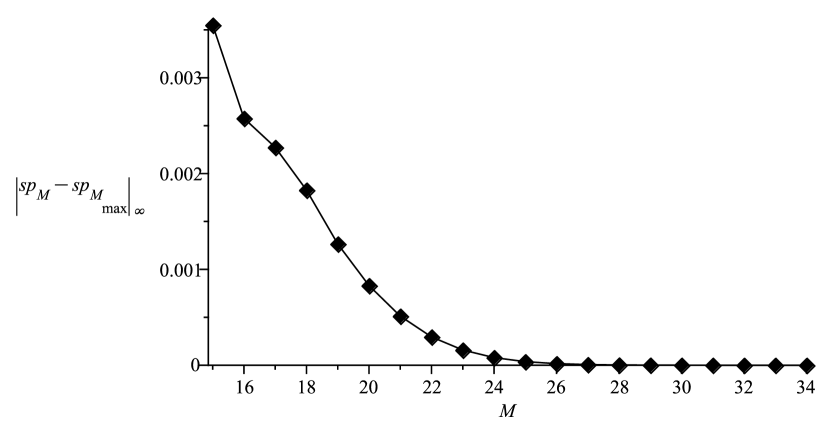
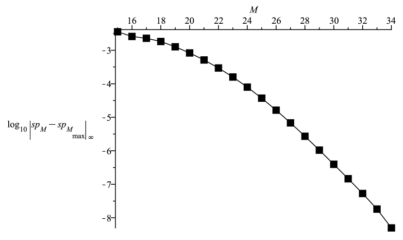
Our first experiment is to test the validity of the truncation (95). Taking and , Formula (95) gives , which corresponds to a matrix of size . In Figure 1, we vary around that value, and plot the norm of the difference between the spectrum below computed with the given value (that is, using the matrix obtained from the basis ) and the spectrum computed using the largest (here ). This experiment confirms that the value predicted by (95) is large enough to obtain a very good accuracy.
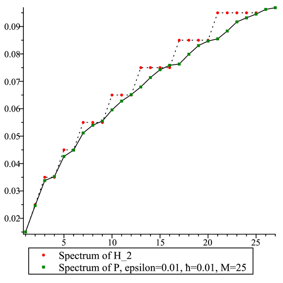
In Figure 2, we compare the spectrum of obtained with the above numerical method to the spectrum of the unperturbed harmonic oscillator . Recall that the oscillator spectrum is explicit
| (96) |
and features the famous phenomemon of clustering of eigenvalues on the ladder , which correspond to polyads in the chemistry literature. While we can recognize the footprints of these polyads on the spectrum of , we notice that much of the structure is lost, even for relatively small .
5.2 has a global minimum
Our goal is to compare the spectrum of with what the -Birkhoff-Gustavson normal form gives. In order to apply our results, let us first check that has a unique non-degenerate minimum, when the constants are properly chosen.
Proposition 5.1
Assume that, in addition to (93), the following conditions hold:
| (97) | |||
| (98) |
Then, the potential admits a unique non-degenerate minimum at the origin. In particular, if and is small enough, then admits a unique non-degenerate minimum at the origin.
Proof . We simply complete three squares: first, we write
Then, we use
Incorporating the last term with the monomial from , we finally write, with ,
This finally gives
| (99) | ||||
| (100) |
Thus, under the conditions of the proposition, we have a sum of four non-negative terms; the sum vanishes if and only if all terms vanish, which is equivalent to .
Now, if and are fixed, the two conditions take the form
| (101) | |||
| (102) |
which holds, if is small enough, as soon as
which is stronger than the first condition .
Remark 5.2 We don’t claim that the two conditions of Proposition 5.1 are necessary. But they allow for a simple proof, and they are sufficient for our numerical purposes and .
5.3 Joint spectrum of and
Let us apply the -Birkhoff-Gustavson normal form of Theorem 3.3 to order 3: we conjugate the initial Schrödinger operator to an operator of the form , and our goal is perform numerical computations neglecting the term.
The operator can be explicitly implemented thanks to Theorem 3.5, Theorem 3.6 and Theorem 4.2. For any given , we obtain the exact matrix for in the orthonormal basis (74), of cardinal .
In order to obtain an approximation of the spectrum of , following Section 4, we fix some energy , and we compute the spectrum of restricted to the spectral subspace of corresponding to energies in , where is fixed. In view of the Bargmann representation of Section 4.2, this is equivalent to computing the spectrum of the restriction of to the space , see (74), for some large enough. Specifically, the integer has to be chosen such that does not intersect the interval for all .
A nice way of displaying this computation is to plot the joint spectrum of the commuting operators and : this is the set of pairs such that, with the notation of Theorem 4.2,
| (103) | ||||
| (104) |
see Figure 7. Then, the spectrum is obtained from the joint spectrum by applying the map .
Notice that the computation of the joint spectrum is much faster than the computation of the spectrum of from Section 5.1, since instead of a matrix of size at least , we have matrices of sizes , so we gain (at least) an order of magnitude in . For instance, with , instead of a matrix, we have 10 matrices of sizes .
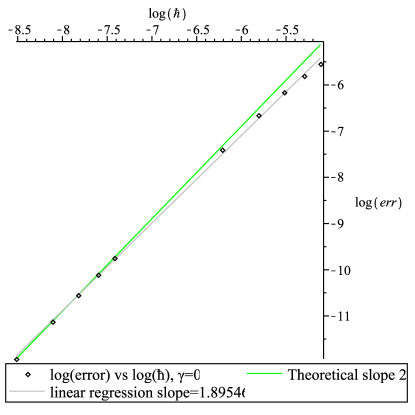
5.4 The case
The case is interesting because the remaining terms of order 3 in the potential , namely and , are completely cancelled out by the Birkhoff normal form: we have in Theorem 3.6. Therefore, the spectrum of is approximated up to merely by the quadratic term , whose spectrum is explicit:
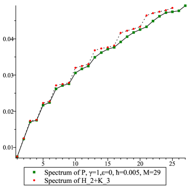
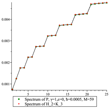
When , the theoretical results of [3] apply. In particular, in the regime , the spectrum should converge to the polyads of (96), with an error of order . This is clearly illustrated in Figures 3 and 4.
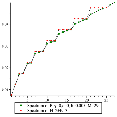
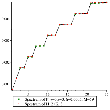
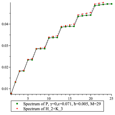
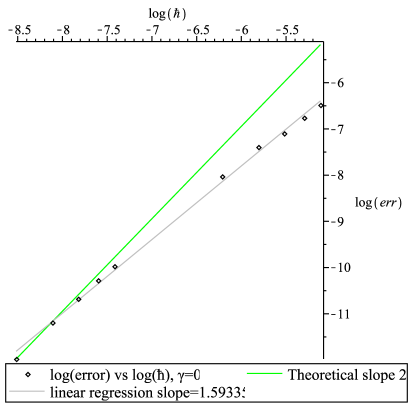
In order to experiment the case , we chose the regime , where we still expect an error of order , which is confirmed by the numerics, see Figures 5 and 6.

The joint spectrum of the commuting operators is depicted in Figure 7.

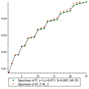
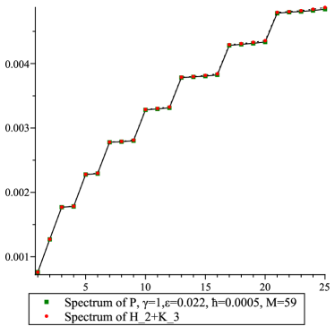
5.5 The case
The case corresponds to the heart of our result, since the Birkhoff term of order 3, is not trivial, due to (94).
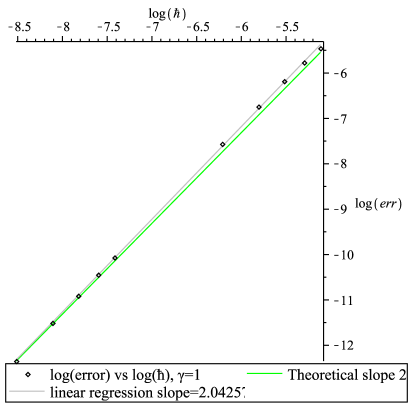
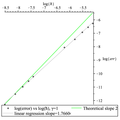
When , as above, the theoretical results of [3] apply and we observe the expected error in Figures 8 and 9. The clear agreement with is a strong confirmation of the validity of the Birkhoff procedure, and in particular of the correctness of the value of from (94), because any other value of would lead to an error of the order of the eigenvalues of on the given spectral subspace, which is known to be .
The new results correspond to . As in the case we experiment the regime , and, in spite of this perturbation, the -Birkhoff-Gustavson procedure suggests that the error should still be . This is confirmed by Figures 10 and 11.
Acknowledgements.
This work is supported in part by funds provided by Henri Lebesgue Center (ANR LEBESGUE), the Laboratory of Fundamental and Applied Mathematics of Oran and the Algerian research project: PRFU No: C00L03ES310120220001. The second author is happy to acknowledge the excellent working conditions that she was given during several stays at the IRMAR.
References
- [1] V. Bargmann. On a Hilbert space of analytic functions and an associated integral transform I. Comm. Pure Appl. Math., 19:187–214, 1961.
- [2] G. Birkhoff. Dynamical systems. AMS, 1927.
- [3] L. Charles and S. Vũ Ngọc. Spectral asymptotics via the semiclassical birkhoff normal form. Duke Math. J., 143(3):463–511, 2008.
- [4] M. Combescure and D. Robert. Coherent states and applications in mathematical physics. Theoretical and Mathematical Physics. Springer, Dordrecht, 2012.
- [5] R. H. Cushman, H. R. Dullin, H. Hanßmann, and S. Schmidt. The resonance. Regul. Chaotic Dyn., 12(6):642–663, 2007.
- [6] J. J. Duistermaat. Non-integrability of the resonance. Ergodic Theory Dynamical Systems, 4:553–568, 1984.
- [7] B. Eckhardt. Birkhoff-Gustavson normal form in classical and quantum mechanics. J. Phys. A, 19:2961–2972, 1986.
- [8] K. Ghomari, B. Messirdi, and S. Vũ Ngọc. Asymptotic analysis for Schrödinger Hamiltonians via Birkhoff-Gustavson normal form. Asymptotic Analysis, 85:1–28, 2013.
- [9] F. G. Gustavson. On constructing formal integrals of a Hamiltonian system near an equilibrium point. Astron. J., 71:670–686, 1966.
- [10] H. Hanßmann, A. Marchesiello, and G. Pucacco. On the detuned 2:4 resonance. J. Nonlinear Sci., 30(6):2513–2544, 2020.
- [11] M. Hitrik, J. Sjöstrand, and S. Vũ Ngọc. Diophantine tori and spectral asymptotics for non-selfadjoint operators. Amer. J. Math., 169(1):105–182, 2007.
- [12] M. Joyeux. Classical dynamics of the , and resonance Hamiltonians. J. Chem. Phys., 203:281–307, 1996.
- [13] M. Joyeux. Gustavson’s procedure and the dynamics of highly excited vibrational states. J. Chem. Phys., 109:2111–2122, 1998.
- [14] T. Kato. Perturbation theory for linear operators, volume 132 of G.M.W. Springer, second edition, 1980.
- [15] R. Krikorian. On the divergence of Birkhoff normal forms. Publ. Math. Inst. Hautes Études Sci., 135:1–181, 2022.
- [16] V. F. Lazutkin. KAM theory and semiclassical approximations to eigenfunctions, volume 24 of Ergebnisse der Mathematik und ihrer Grenzgebiete (3). Springer-Verlag, Berlin, 1993. With an addendum by A. I. Shnirelman.
- [17] J. Moser. New aspects in the theory of stability of Hamiltonian systems. Comm. Pure Appl. Math., 11:81–114, 1958.
- [18] F. Rellich. Perturbation theory of eigenvalue problems. Assisted by J. Berkowitz. With a preface by Jacob T. Schwartz. Gordon and Breach Science Publishers, New York-London-Paris, 1969.
- [19] J. Sjöstrand. Semi-excited states in nondegenerate potential wells. Asymptotic Analysis, 6:29–43, 1992.
- [20] R. Wordsworth, J. Seeley, and K. Shine. Fermi resonance and the quantum mechanical basis of global warming. The Planetary Science Journal, 5:67, 03 2024.
- [21] N. T. Zung. Convergence versus integrability in Birkhoff normal form. Ann. of Math. (2), 161(1):141–156, 2005.