Numerical Computation of Generalized Wasserstein Distances with Applications to Traffic Model Analysis

Abstract

Generalized Wasserstein distances allow to quantitatively compare two continuous or atomic mass distributions with equal or different total mass. In this paper, we propose four numerical methods for the approximation of three different generalized Wasserstein distances introduced in the last years, giving some insights about their physical meaning. After that, we explore their usage in the context of the sensitivity analysis of differential models for traffic flow. The quantification of models sensitivity is obtained by computing the generalized Wasserstein distances between two (numerical) solutions corresponding to different inputs, including different boundary conditions.

MSC: 76A30; 90C31; 90C90; 35L50; 35L53.

1 Introduction

Context.

In this paper we are concerned with the numerical computation of Wasserstein distance (WD) and Generalized Wasserstein distance (GWD) in the context of traffic flow models. As for all dynamical systems, the study of the sensitivity of the models can be realized measuring the ‘distance’ between two solutions obtained with different inputs (like, e.g., any of the model parameters, initial conditions, boundary conditions, etc.). This allows one to understand their impact on the final solution, and ultimately quantify the degree of chaoticity of the system. The question arises which distance is more suitable to this kind of investigation. It is by now well understood that $L^{p}$ distances do not catch the natural concept of distance among traffic (vehicle) densities, see, e.g., the discussion in [8, Sec. 7.1] and Sec. 2 in this paper, while the WD appears more natural, at least in the context of traffic flow, see, e.g., [3, 8, 9]. The drawback is that WD is limited to balanced mass distribution (equal masses), while real traffic problems often need to consider scenarios with a different amount of vehicles, especially because of different inflow/outflow at boundaries. This suggests to move towards GWDs, which allows to deal with unbalanced mass distributions, but serious computational problems arise: all existing definitions are quite abstract and it is not immediate to derive suitable numerical approximations.

Relevant literature.

A common feature of various optimal transport distances between finite positive Borel measures on a separable complete metric space $(X,\mathfrak{D})$ is that their primal definition requires the minimization of a transportation cost including an additive contribution of the form

$$\int_{X\times X}c(x,y)\,d\gamma\,,$$ (1.1)

where $c:X\times X\to[0,+\infty]$ is a fixed lower semi-continuous cost function.

In the balanced problem, that one considers to define the classical Wasserstein distance between two probability measures $\mu^{\textsc{s}}$ and $\mu^{\textsc{d}}$, the minimization occurs upon transport plans $\gamma$, i.e., probability measures on $X\times X$ with marginals $\mu^{\textsc{s}}$ and $\mu^{\textsc{d}}$. Namely, one considers the projection $\pi^{\textsc{s}}$ (resp., $\pi^{\textsc{d}}$) onto the first (resp., the second) factor of the Cartesian product $X\times X$, and takes as admissible competitors the finite positive measures $\gamma$ for which

$$\pi^{\textsc{s}}_{\,\sharp}\gamma=\mu^{\textsc{s}}\,,\qquad\pi^{\textsc{d}}_{\,\sharp}\gamma=\mu^{\textsc{d}}\,,$$ (1.2)

where $\pi^{\textsc{s}}_{\,\sharp}\gamma$ (resp., $\pi^{\textsc{d}}_{\,\sharp}\gamma$) denotes the push-forward measure of $\gamma$ under $\pi^{\textsc{s}}$ (resp., $\pi^{\textsc{d}})$.

In order to define distances between finite positive measures on a bounded open set $\Omega$ in a finite dimensional Euclidean space, there exist various approaches to similar, but unbalanced, problems, that correspond each to the appropriately constrained minimization of a specific objective functional. In this paper we focus on four of such approaches.

1. The approach by Figalli & Gigli [11], which consists in minimizing the integral cost (1.1) among all finite positive measures $\gamma$ on $\overline{\Omega}\times\overline{\Omega}$ whose marginals induce on $\Omega$ the prescribed finite positive Borel measures.

2. The approach by Piccoli & Rossi [19], which includes in the definition of the functional the additive contributions

   $$|\pi^{\textsc{s}}_{\,\sharp}\gamma-\mu^{\textsc{s}}|(\Omega)+|\pi^{\textsc{d}}_{\,\sharp}\gamma-\mu^{\textsc{d}}|(\Omega)\,,$$ (1.3)

   in addition to (1.1), with the minimization occurring upon finite positive Borel measures on $\Omega\times\Omega$.

3. A third approach relies on the logarithmic entropy-transport distance that was independently introduced by Kondratyev, Monsaingeon & Vorotnikov in [14], by Chizat, Peyré, Schmitzer & Vialard in [6, 7], and by Liero, Mielke & Savaré in [15], called Hellinger–Kantorovich or Wasserstein–Fisher–Rao distance. This approach also relies on the minimization, among finite positive Borel measures on $\Omega\times\Omega$, of a perturbation of (1.1), except that the penalization (1.3) is replaced by

   $$\int_{\Omega}\Big{(}\sigma^{\textsc{s}}\log(\sigma^{\textsc{s}})-\sigma^{\textsc{s}}+1\Big{)}\,d\mu^{\textsc{s}}+\int_{\Omega}\Big{(}\sigma^{\textsc{d}}\log(\sigma^{\textsc{d}})-\sigma^{\textsc{d}}+1\Big{)}\,d\mu^{\textsc{d}}\,,$$ (1.4)

   if $d(\pi^{\textsc{s}}_{\,\sharp}\gamma)=\sigma^{\textsc{s}}\,d\mu^{\textsc{s}}$ and $d(\pi^{\textsc{d}}_{\,\sharp}\gamma)=\sigma^{\textsc{d}}\,d\mu^{\textsc{d}}$ for appropriate densities $\sigma^{\textsc{s}}$ and $\sigma^{\textsc{d}}$, and $+\infty$ otherwise. (Incidentally, a similar objective, in which an entropic regularization is added to (1.1) and (1.4), in considered in [18], where the appropriate dual formulation of the problem is addressed by Sinkhorn iterations.)

4. A fourth approach relates to the contribution by Savaré & Sodini [23], in which the logarithmic entropy transport distance is characterized, in its various equivalent formulations, by convex relaxation. In particular, their approach can be considered the natural one to numerically approximate the (Gaussian) Hellinger–Kanrotovich distance in its homogeneous formulation.

We point out that the last two approaches only differ numerically, as in principle the corresponding unbalanced optimal transport formulations are analytically equivalent. Both extend WD to the cone of non-negative Borel measures of finite mass that are different from zero (see Rem. 5 below). On the contrary, the first two approaches do give an extension of WD, despite defining a distance on the cone (see Rems. 3 and 4 below). We recall that no extension of WD to the set of signed measures can define a distance [17].

Main contribution.

This paper has multiple goals: first of all, the four approaches are recalled and compared at the theoretical level, so to have a common and exhaustive reference for all recent developments about GWDs.

Second, four new ad hoc computational methods are devised in order to practically compute the four GWDs (actually they are three GWDs, since two of them coincide under suitable assumptions). The methods are individually studied and their main properties are discussed through some explanatory numerical tests.

Third, the four approaches are compared on the same academic test in order to understand which one is the most suitable in the context of traffic flow models.

Finally, the three most promising approaches are further compared on three realistic traffic problems.

Anticipating the conclusions, we can say that Figalli & Gigli approach appears to be preferable among all, mainly for two reasons: (i) it is the most manageable from the computational point of view (easy to code, fast computation), and (ii) it is the most informative on the modeling side.

Plan of the paper.

The paper is organized as follows. In Sect. 2 we recall the main motivations of the paper and we set up notations for linear programming and discrete-to-discrete optimal mass transport. In Sect. 3 we recall the definition and the basic properties of some known unbalanced optimal transport-type distances between positive Borel measures of finite mass, along with indications for their numerical computation in the discrete-to-discrete case. In Sect. 4 we test the actual implementation of the aforementioned computational approaches, their interplay with the numerical boundary, and their capability to detect significant patterns, with examples in which the exact value of the distances is available analytically. In Sect. 5 these conclusions are applied in the context of traffic analysis in order to achieve various goals: (i) to assess the impact of boundary conditions, (ii) to evaluate the sensitivity to traffic lights frequency variations, and (iii) to compare forecasts depending on whether or not the model takes inertial effects into account.

2 The Wasserstein distance in the context of vehicular traffic

2.1 Motivations

Usually the quantification of the closeness of two time-dependent distributions is performed by means of the $L^{1}$, $L^{2}$ or $L^{\infty}$ distance (in space at final time or in both space and time). Although this can be satisfactory for nearly equal outputs or for convergence results, it appears inadequate for measuring the distance of largely different outputs. To see this, let us focus on the example depicted in Fig. 1, where

\begin{overpic}[width=202.3529pt]{figs/L1vsW} \put(17.0,60.0){$\rho^{1}$}\put(41.5,60.0){$\rho^{2}$}\put(66.0,60.0){$\rho^{3}$} \end{overpic}

Figure 1: Three density functions with disjoint supports.

three density functions $\rho^{i}$, $i=1,2,3$, corresponding to the same total mass, say $M$, are plotted. It is plain that the $L^{1}$ distances between $\rho_{1}$ and $\rho_{2}$ and between $\rho_{1}$ and $\rho_{3}$ are both equal to $2M$. Similarly, all $L^{p}$ distances are blind with respect to variation of the densities once the supports of them are disjoint. Our perception of distance suggests instead that $\|\rho_{3}-\rho_{1}\|>\|\rho_{2}-\rho_{1}\|$, and this is exactly what Wasserstein distance guarantees, as we will see in the next section.

2.2 Basic theory

Let us denote by $(X,\mathfrak{D})$ a locally compact complete and separable metric space with distance $\mathfrak{D}$, and by $\mathcal{B}(X)$ the Borel $\sigma$-algebra of $(X,\mathfrak{D})$. Let us also denote by $\mathcal{M}^{+}(X)$ the set of non-negative finite measures on $(X,\mathcal{B}(X))$. Let $\mu^{\textsc{d}}$ (d standing for demand or destination) and $\mu^{\textsc{s}}$ (s standing for supply or source) be two Radon measures in $\mathcal{M}^{+}(X)$ such that $\mu^{\textsc{d}}(X)=\mu^{\textsc{s}}(X)$ (same total mass).

Definition 1 (Wasserstein distance).

For any $p\in[1,+\infty)$, the $L^{p}$-Wasserstein distance between $\mu^{\textsc{s}}$ and $\mu^{\textsc{d}}$ is

$$W_{p}(\mu^{\textsc{s}},\mu^{\textsc{d}}):=\left(\inf_{\gamma\in\Gamma(\mu^{\textsc{s}},\mu^{\textsc{d}})}\int_{X\times X}\mathfrak{D}(x,y)^{p}\ d\gamma(x,y)\right)^{1/p}$$ (2.1)

where $\Gamma$ is the set of transport plans connecting $\mu^{\textsc{s}}$ to $\mu^{\textsc{d}}$, i.e.

$$\Gamma(\mu^{\textsc{s}},\mu^{\textsc{d}}):=\left\{\gamma\in\mathcal{Q}^{+}(X\times X)\text{ s.t. }\gamma(A\times X)=\mu^{\textsc{s}}(A),\ \gamma(X\times B)=\mu^{\textsc{d}}(B),\ \forall\ A,B\in\mathcal{B}(X)\right\}.$$

Remark 1.

The distance defined by (2.1) makes sense for any two given measures $\mu^{\textsc{s}}$ and $\mu^{\textsc{d}}$ on a finite dimensional normed space, whether they are absolutely continuous or not with respect to the Lebesgue measure.

It is well known that the notion of Wasserstein distance can be put in relation with the Monge–Kantorovich optimal mass transfer problem [26]: a pile of, say, soil, has to be moved to an excavation with same total volume. Moving a unit quantity of mass has a cost which equals the distance between the source and the destination point. We consequently are looking for a way to rearrange the first mass onto the second which requires minimum cost.

Remark 2.

In our framework, the mass to be moved corresponds to that of vehicles. We therefore measure the distance between two traffic density distributions by computing the minimal cost to rearrange vehicles from the first configuration onto the second one. We also stress that, since we are considering macroscopic models, vehicles are indistinguishable so we are not able to pinpoint the exact same vehicle in the two scenarios, cf. [9].

In the particular case of 1D optimal transport various characterizations give alternative, more manageable, definitions of WD. For example, if $(X,\mathfrak{D})$ is $\mathbb{R}$ with the euclidean distance $|\cdot|$, then, in the case of two Dirac delta functions $\delta_{x}$, $\delta_{y}$ we simply have $W_{p}(\delta_{x},\delta_{y})=\mathfrak{D}(x,y):=|y-x|$. That coincides with the desired distance quantification in the case of only two vehicles on a road, located in $x$ and $y$ respectively. Instead, in the case of two absolutely continuous measures with $d\mu^{\textsc{s}}=\rho^{\textsc{s}}dx$ and $d\mu^{\textsc{d}}=\rho^{\textsc{d}}dx$, by [25, Rem. 2.19] we have

$$W_{1}(\mu^{\textsc{s}},\mu^{\textsc{d}})=\int_{\mathbb{R}}|F^{\textsc{s}}(x)-F^{\textsc{d}}(x)|dx=\int_{\mathbb{R}}\big{|}(F^{\textsc{s}})^{-1}(x)-(F^{\textsc{d}})^{-1}(x)\big{|}dx,$$ (2.2)

with

$$F^{\textsc{s}}(x):=\int_{-\infty}^{x}\rho^{\textsc{s}}(z)dz,\quad F^{\textsc{d}}(x):=\int_{-\infty}^{x}\rho^{\textsc{d}}(z)dz$$ (2.3)

for $p=1$, whereas for $p\geq 1$,

$$W_{p}(\mu^{\textsc{s}},\mu^{\textsc{d}})=\left(\int_{\mathbb{R}}|T^{*}(x)-x|^{p}\ \rho^{\textsc{s}}(x)dx\right)^{1/p},$$ (2.4)

where $T^{*}:\mathbb{R}\to\mathbb{R}$ satisfies

$$\int_{-\infty}^{x}\rho^{\textsc{s}}(z)dz=\int_{-\infty}^{T^{*}(x)}\rho^{\textsc{d}}(z)dz\quad\forall x\in\mathbb{R}.$$ (2.5)

Eqs. (2.4)-(2.5) translate the fundamental property of monotone rearrangement of the mass [25, Rem. 2.19], i.e. the optimal strategy consists in transferring the mass starting from the left, see Fig. 2.

\begin{overpic}[width=404.71353pt]{figs/monotonerearrangement} \put(13.0,0.0){$x$} \put(72.0,0.0){$T^{*}(x)$} \put(25.0,14.0){$\rho^{\textsc{s}}$} \put(83.0,16.0){$\rho^{\textsc{d}}$} \end{overpic}

Figure 2: Property of monotone rearrangement.

2.3 Numerical setting

Let us introduce here the numerical setting that will accompany us throughout the paper, see Fig. 3.

Figure 3: Numerical setting for a generic one-dimensional problem. Two copies of the domain $X$ with supply mass only (left) and demand mass only (right).

For simplicity, we will only consider the one-dimensional interval $X=[x_{\textsc{min}},x_{\textsc{max}}]$, divided in $N$ equispaced cells $C_{1},\ldots,C_{N}$ ($N$ is our first parameter of discretization, and we expect to vanish the numerical error for $N\to+\infty$). We also denote by $x_{i}$ the barycenter of the cell $C_{i}$, $i=1,\ldots,N$ and by $\Delta x:=x_{i+1}-x_{i}$ the step of the space discretization. To measure the distance between two cells $C_{i}$ and $C_{j}$, we will always use the Euclidean norm $\mathfrak{D}(x_{j},x_{k}):=|x_{k}-x_{j}|$.

Moving to the masses, for any $i=1,\ldots,N$ we denote by

$$m^{\textsc{s}}_{i}:=\rho^{\textsc{s}}(x_{i})\Delta x,\qquad m^{\textsc{d}}_{i}:=\rho^{\textsc{d}}(x_{i})\Delta x,$$ (2.6)

the supply and the demand mass located in $C_{i}$, respectively. Roughly speaking, this corresponds to concentrate the masses on specific points, thus getting purely atomic density distributions $\hat{\rho}^{\textsc{s}}:=\sum_{i}m_{i}^{\textsc{s}}\delta_{x_{i}}$ and $\hat{\rho}^{\textsc{d}}:=\sum_{i}m_{i}^{\textsc{d}}\delta_{x_{i}}$ where $\delta$ denotes the Dirac delta. Note that, in our context, the vectors $\{m_{i}^{\textsc{s}}\}_{i}$ and $\{m_{i}^{\textsc{d}}\}_{i}$ will be given. Moreover, to avoid any confusion between theoretical and numerical boundary conditions we will always assume that

$$m_{1}^{\textsc{s}}=m_{N}^{\textsc{s}}=m_{1}^{\textsc{d}}=m_{N}^{\textsc{d}}=0,$$ (2.7)

in such a way that boundaries remain out of play.

For some reasons which will be clear later on, it is also useful defining the remaining supply mass at $C_{i}$, denoted by $\mathring{m}^{\textsc{s}}_{i}$, and the remaining demand mass at $C_{i}$, denoted by $\mathring{m}^{\textsc{d}}_{i}$, $i=1,\ldots,N$.

In order to get a numerical approximation of the WD in $\mathbb{R}^{1}$, it is convenient to resort to the definition (2.2). Indeed, any quadrature formula is suitable to get the desired value with arbitrary precision, provided $\rho^{\textsc{s},\textsc{d}}$ are sufficiently smooth and $N$ is sufficiently large. For example, the naive composite mid-point formula gives

$$W_{1}(\rho^{\textsc{s}},\rho^{\textsc{d}})\approx\tilde{W}_{1}(m^{\textsc{s}},m^{\textsc{d}}):=\Delta x\sum_{j=1}^{N}\left|\sum_{i=1}^{j}m_{i}^{\textsc{s}}-\sum_{i=1}^{j}m_{i}^{\textsc{d}}\right|.$$ (2.8)

The case of more general spaces, including networks embedded in $\mathbb{R}^{2}$, is more difficult. Typically the problem is solved by reformulating it in a fully discrete setting as a Linear Programming (LP) problem. The interested reader can find in the books by Santambrogio [22, Sect. 6.4.1] and Sinha [24, Chapt. 19] the complete procedure, recently used also in the context of traffic flow on networks [3]. Even if we will stick with the one-dimensional case, we recall now the crucial steps of this approach because it will be useful in the following.

Following the mass transport interpretation, let $c_{jk}$ be the cost of shipping a unit quantity of mass from the source $C_{j}$, $j=1,\ldots,N$, to the destination $C_{k}$, $k=1,\ldots,N$. In general, $c_{jk}$ is usually defined as the length of the shortest path joining $x_{j}$ and $x_{k}$. Let $\gamma_{jk}$ be the (unknown) quantity shipped from the source $j$ to the destination $k$. The problem is then formulated as

minimize $$\sum\limits_{j=1}^{N}\sum\limits_{k=1}^{N}c_{jk}\gamma_{jk}$$

subject to

.

(2.9)

The solution gives an approximation $\tilde{W}_{1}$ of $W_{1}$. Note that the solution satisfies $\gamma_{jk}\leq\min\{m^{\textsc{s}}_{j},m^{\textsc{d}}_{k}\}$ since one cannot move more than $m^{\textsc{s}}_{j}$ from any source $j$ and it is useless to bring more than $m^{\textsc{d}}_{k}$ to any destination $k$. From (2.9), it is easy to recover a standard LP problem with equality constraints

minimize $$\mathbf{c}^{\intercal}\mathbf{x}$$

subject to

,

(2.10)

simply defining

$$\begin{array}[]{l}\mathbf{x}:=(\gamma_{11},\gamma_{12},\ldots,\gamma_{1N},\gamma_{21},\gamma_{22},\ldots,\gamma_{2N},\ldots,\gamma_{N1},\ldots,\gamma_{NN})^{\intercal}\\ \mathbf{c}:=(c_{11},c_{12},\ldots,c_{1N},c_{21},c_{22},\ldots,c_{2N},\ldots,c_{N1},\ldots,c_{NN})^{\intercal}\\ \mathbf{b}:=(m^{\textsc{s}}_{1},\ldots,m^{\textsc{s}}_{N},m^{\textsc{d}}_{1},\ldots,m^{\textsc{d}}_{N})^{\intercal}\end{array}$$ (2.11)

and $\mathbf{A}$ as the $2N\times N^{2}$ block matrix

$$\mathbf{A}:=\left[\begin{array}[]{ccccc}\mathbb{1}_{\!N}&\mathbb{0}_{\!N}&\mathbb{0}_{\!N}&\cdots&\mathbb{0}_{\!N}\\ \mathbb{0}_{\!N}&\mathbb{1}_{\!N}&\mathbb{0}_{\!N}&\cdots&\mathbb{0}_{\!N}\\ \mathbb{0}_{\!N}&\mathbb{0}_{\!N}&\mathbb{1}_{\!N}&\cdots&\mathbb{0}_{\!N}\\ \vdots&\vdots&\vdots&\ddots&\vdots\\ \mathbb{0}_{\!N}&\mathbb{0}_{\!N}&\mathbb{0}_{\!N}&\cdots&\mathbb{1}_{\!N}\\ I_{N}&I_{N}&I_{N}&I_{N}&I_{N}\\ \end{array}\right],$$ (2.12)

where $I_{N}$ is the $N\times N$ identity matrix, $\mathbb{1}_{\!N}:=(\underbrace{1\ 1\ \cdots\ 1}_{N\text{ times}})$, and $\mathbb{0}_{\!N}:=(\underbrace{0\ 0\ \cdots\ 0}_{N\text{ times}})$.

3 Generalized Wasserstein distances

We recall some definitions of metrics on the space of positive finite Borel measures on the locally compact complete and separable metric space $(X,\mathfrak{D})$, inducing the weak-narrow convergence, all inspired to the distance defined by (2.1) between probability measures.

3.1 Figalli & Gigli approach [11]

3.1.1 Basic theory

In [11], an optimal transport type distance is introduced, with respect to which the heat equation under Dirichlet conditions at the boundary of an open bounded domain $\Omega$ can be described as the gradient flow of an entropy, similarly to the case of the heat equation in free space. In order to encode the correct boundary conditions in the minimizing movement scheme, the GWD between two finite non-negative (Borel) measures $\mu^{\textsc{s}},\mu^{\textsc{d}}$ on $\Omega$ is defined by

$$W^{\textsc{fg}}_{p}(\mu^{\textsc{s}},\mu^{\textsc{d}})=\left\{\inf_{\gamma}\int_{\,\overline{\Omega}\times\overline{\Omega}}\|x-y\|^{p}d\gamma(x,y)\right\}^{\frac{1}{p}},$$ (3.1)

where infimum is over

$$\Big{\{}\gamma\in\mathcal{M}^{+}(\overline{\Omega}\times\overline{\Omega})\ \Big{|}\ \big{(}\pi^{\textsc{s}}_{\,\,\sharp}\gamma\big{)}\mathbin{\vrule height=6.88889pt,depth=0.0pt,width=0.55974pt\vrule height=0.55974pt,depth=0.0pt,width=5.59721pt}\Omega=\mu^{\textsc{s}}\,,\ \big{(}\pi^{\textsc{d}}_{\,\,\sharp}\gamma\big{)}\mathbin{\vrule height=6.88889pt,depth=0.0pt,width=0.55974pt\vrule height=0.55974pt,depth=0.0pt,width=5.59721pt}\Omega=\mu^{\textsc{d}}\Big{\}}\,.$$ (3.2)

In the latter, we used the notation $(\bar{\mu}\mathbin{\vrule height=6.88889pt,depth=0.0pt,width=0.55974pt\vrule height=0.55974pt,depth=0.0pt,width=5.59721pt}\Omega)(A)=\bar{\mu}(A\cap\Omega)$ for the restriction to $\Omega$ of a measure $\bar{\mu}$ on $\overline{\Omega}$, and for all given $\gamma$ we denoted by $\pi^{\textsc{s}}_{\,\,\sharp}\gamma$ (resp., $\pi^{\textsc{d}}_{\,\,\sharp}\gamma$) the push-forward of $\gamma$ under the projection defined on $\overline{\Omega}\times\overline{\Omega}$ by $\pi^{\textsc{s}}(x,y)=x$ (resp., $\pi^{\textsc{d}}(x,y)=y$). Equivalently, a non-negative finite Radon measure $\gamma$ on $\overline{\Omega}\times\overline{\Omega}$ is an admissible competitor for the minimization in (3.1) if and only if

$$\gamma(A\times\overline{\Omega})=\mu^{\textsc{s}}(A)\,,\ \gamma(\overline{\Omega}\times B)=\mu^{\textsc{d}}(B)\,,\qquad\text{for all $A,B\in\mathcal{B}(\Omega)$.}$$ (3.3)

Let us note that (3.2) coincides with the set

$$\bigcup_{({\overline{\mu}}^{\textsc{s}},{\overline{\mu}}^{\textsc{d}})}\Big{\{}\gamma\in\mathcal{M}^{+}(\overline{\Omega}\times\overline{\Omega})\ \Big{|}\ \pi^{\textsc{s}}_{\,\sharp}\gamma={\bar{\mu}}^{\textsc{s}}\,,\ \pi^{\textsc{d}}_{\,\sharp}\gamma={\bar{\mu}}^{\textsc{d}}\Big{\}},$$

where the union is over all pairs $({\bar{\mu}}^{\textsc{s}},{\bar{\mu}}^{\textsc{d}})\in\mathcal{M}^{+}(\overline{\Omega})\times\mathcal{M}^{+}(\overline{\Omega})$ such that

$${\bar{\mu}}^{\textsc{s}}\mathbin{\vrule height=6.88889pt,depth=0.0pt,width=0.55974pt\vrule height=0.55974pt,depth=0.0pt,width=5.59721pt}\Omega=\mu^{\textsc{s}}\,,\ {\bar{\mu}}^{\textsc{d}}\mathbin{\vrule height=6.88889pt,depth=0.0pt,width=0.55974pt\vrule height=0.55974pt,depth=0.0pt,width=5.59721pt}\Omega=\mu^{\textsc{d}}\,,\ {\bar{\mu}}^{\textsc{s}}(\overline{\Omega})={\bar{\mu}}^{\textsc{d}}(\overline{\Omega})\,.$$

Hence, an equivalent variational definition of the unbalanced optimal transport distance (3.1) is

$$\min\Big{\{}W_{p}({\bar{\mu}}^{\textsc{s}},{\bar{\mu}}^{\textsc{d}})\ \Big{|}\ {\bar{\mu}}^{\textsc{s}}\mathbin{\vrule height=6.88889pt,depth=0.0pt,width=0.55974pt\vrule height=0.55974pt,depth=0.0pt,width=5.59721pt}\Omega=\mu^{\textsc{s}}\,,\ {\bar{\mu}}^{\textsc{d}}\mathbin{\vrule height=6.88889pt,depth=0.0pt,width=0.55974pt\vrule height=0.55974pt,depth=0.0pt,width=5.59721pt}\Omega=\mu^{\textsc{d}}\,,\ {\bar{\mu}}^{\textsc{s}}(\partial\Omega)-{\bar{\mu}}^{\textsc{d}}(\partial\Omega)=\mu^{\textsc{s}}(\Omega)-\mu^{\textsc{d}}(\Omega)\Big{\}},$$ (3.4)

where the classical WD is defined as in (2.1) with $\mathfrak{D}(x,y)=\|x-y\|$ for probability measures, and extended by homogeneity to non-negative Radon measures with equal masses. With this definition, if $\bar{\mu}^{\textsc{s}},\bar{\mu}^{\textsc{d}}\in\mathcal{M}^{+}(\overline{\Omega})$ are fixed, then $W_{p}(t\bar{\mu}^{\textsc{s}},t\bar{\mu}^{\textsc{d}})$ is arbitrarily large if $t>0$ is large enough. Hence the minimum in (3.4) is indeed achieved. Notice that mass unbalance $\mu^{\textsc{s}}(\Omega)-\mu^{\textsc{d}}(\Omega)$ is fixed if so are the marginals $\mu^{\textsc{s}}$ and $\mu^{\textsc{d}}$.

The authors of [11] deal explicitly with the case of a quadratic unitary cost, i.e., $c(x,y)=\|x-y\|^{2}$ in (3.1), but their main results also hold for a more general cost, e.g., $c(x,y)=\|x-y\|^{p}$, with $p\geq 1$. As intermediate steps towards their main results, they prove lower semicontinuity with respect to the weak-$\ast$ convergence on $\Omega$ and provide a gluing lemma implying the triangle inequality, so that (3.1) defines a distance on $\mathcal{M}^{+}(\Omega)$, and the infimum is achieved by an appropriate optimal plan $\gamma$.

The idea of minimizing (3.1) among all $\gamma$ as in (3.2) is that $\partial\Omega$ models an infinite mass reservoir “at infinity” and the transportation policy described by convenient competitors $\gamma$ might include the option to cut out part of the material from the actual transference plan, by transferring it to $\partial\Omega$, as well as the possibility to integrate the transportation plan by transferring material from $\partial\Omega$ to the final destination, provided that the transportation cost to and from $\partial\Omega$ is accounted for in the overall integral cost together with that of moving the mass that is authentically transported. A dual formulation of the problem leads to a generalization of Kantorovich potentials and Kantorovich norms, which had been already investigated especially in the case of a linear cost ($p=1$), see [12, 13].

Remark 3.

It is clear from (3.4) that the distance between positive finite Radon measures introduced in [11] is not an extension of the classical Wasserstein distance: if the two prescribed marginals are concentrated close to the boundary with supports far apart from each other, then while solving (3.4) there will be a convenience for $\bar{\mu}^{\textsc{s}}$ and $\bar{\mu}^{\textsc{d}}$ in charging appropriately two corresponding disjoint boundary regions, after which the Wasserstein to be minimized will be achieved by transport plans that only move mass from or to the boundary. In fact, the goal of [11] was to generalize Otto’s calculus to PDEs under Dirichlet conditions, rather than extending the optimal transport metrics to finite positive Radon measures.

In the special case of two purely atomic marginals with finite supports in a one-dimensional domain, i.e.,

$$\mu^{\textsc{s}}=\sum_{i=2}^{N-1}m_{i}^{\textsc{s}}\delta_{x_{i}}\,,\qquad\mu^{\textsc{d}}=\sum_{i=2}^{N-1}m_{i}^{\textsc{d}}\delta_{x_{i}}$$

we get an interpretation of (3.4) as a linear programming problem. Namely, we consider the problem

$$\min_{(m_{1}^{\textsc{s}},m_{N}^{\textsc{s}},m_{1}^{\textsc{d}},m_{N}^{\textsc{d}})\in\mathbb{R}^{4}}\left\{W_{p}^{p}\Big{(}\sum_{i=1}^{N}m_{i}^{\textsc{s}}\delta_{x_{i}}\mathbin{,}\sum_{i=1}^{N}m_{i}^{\textsc{d}}\delta_{x_{i}}\Big{)}\ \Big{|}\ m_{1}^{\textsc{s}}+m_{N}^{\textsc{s}}-(m_{1}^{\textsc{d}}+m_{N}^{\textsc{d}})=\Delta M\right\}\,,$$

where

$$\Delta M:=\sum_{i=2}^{N-1}m_{i}^{\textsc{s}}-\sum_{i=2}^{N-1}m_{i}^{\textsc{d}},$$

and, after setting $c_{jk}=\|x_{j}-x_{k}\|^{p}$, for all $j,k\in\{1,\ldots,N\}$, we write it in the equivalent form

$$\begin{split}\tilde{W}^{\textsc{fg}}_{1}(m^{\textsc{s}},m^{\textsc{d}}):=\min\Bigg{\{}\sum_{j,k=1}^{N}c_{jk}\gamma_{jk}\ \Big{|}\ \gamma\in[0,+\infty)^{N\times N}\,,\ &\sum_{k=1}^{N}\gamma_{jk}=m_{j}^{\textsc{s}}\,,\ \text{for $j\in\{2,\ldots,N-1\}$}\,,\\ &\sum_{j=1}^{N}\gamma_{jk}=m_{k}^{\textsc{d}}\,,\ \text{for $k\in\{2,\ldots,N-1\}$},\\ &\sum_{k=1}^{N}\big{(}\gamma_{1k}+\gamma_{Nk}\big{)}-\sum_{j=1}^{N}\big{(}\gamma_{j1}+\gamma_{jN}\big{)}=\Delta M\Bigg{\}}^{\frac{1}{p}}\,.\end{split}$$

That amounts to the minimization of a linear objective in a convex polytope obtained by intersecting $2N-3$ affine half-spaces in $\mathbb{R}^{N\times N}$ with $[0,+\infty)^{N\times N}$. Alternatively, the last constraint may be converted into an additional contribution to the total cost involving suitable Lagrange multipliers.

3.1.2 Computational approach

The minimization problem introduced in the previous section can be formulated as a LP problem in the standard form (2.10) defining

$$\mathbf{x}:=(\gamma_{11},\gamma_{12},\ldots,\gamma_{1N},\gamma_{21},\gamma_{22},\ldots,\gamma_{2N},\ldots,\gamma_{N1},\ldots,\gamma_{NN})^{\intercal}$$

$$\mathbf{c}:=(c_{11},c_{12},\ldots,c_{1N},c_{21},c_{22},\ldots,c_{2N},\ldots,c_{N1},\ldots,c_{NN})^{\intercal}$$

$$\mathbf{b}:=(m^{\textsc{s}}_{2},\ldots,m^{\textsc{s}}_{N-1},m^{\textsc{d}}_{2},\ldots,m^{\textsc{d}}_{N-1},\Delta M)^{\intercal}$$

and $\mathbf{A}$ as the $(2N-3)\times N^{2}$ block matrix

$$\mathbf{A}:=\left[\begin{array}[]{cccccc}\mathbb{0}_{\!N}&\mathbb{1}_{\!N}&\mathbb{0}_{\!N}&\cdots&\mathbb{0}_{\!N}&\mathbb{0}_{\!N}\\ \mathbb{0}_{\!N}&\mathbb{0}_{\!N}&\mathbb{1}_{\!N}&\cdots&\mathbb{0}_{\!N}&\mathbb{0}_{\!N}\\ \vdots&\vdots&\vdots&\ddots&\vdots&\vdots\\ \mathbb{0}_{\!N}&\mathbb{0}_{\!N}&\mathbb{0}_{\!N}&\cdots&\mathbb{1}_{\!N}&\mathbb{0}_{\!N}\\ J_{N}&J_{N}&J_{N}&\cdots&J_{N}&J_{N}\\ U_{N}&Z_{N}&Z_{N}&\cdots&Z_{N}&U_{N}\end{array}\right],$$ (3.5)

where $I_{N}$ is the $N\times N$ identity matrix, $\mathbb{1}_{\!N}:=(\underbrace{1\ 1\ \cdots\ 1}_{N\text{ times}})$, $\mathbb{0}_{\!N}:=(\underbrace{0\ 0\ \cdots\ 0}_{N\text{ times}})$, $Z_{N}:=(-1\ \underbrace{0\ 0\ \cdots\ 0}_{N-2\text{ times}}-1)$, $U_{N}:=(0\ \underbrace{1\ 1\ \cdots\ 1}_{N-2\text{ times}}\ 0)$, and $J_{N}$ is the $(N-2)\times N$ block matrix $[\mathbb{0}_{\!N-2}^{\intercal}\ I_{N-2}\ \mathbb{0}_{\!N-2}^{\intercal}]$.

The PL formulation described above can be reformulated in an almost equivalent form, which is actually more similar to the problem (2.9) and also allows for a nice, further, generalization. Still keeping the simplifying assumption (2.7), the vector $\mathbf{x}$ of the unknowns is modified adding four new unknowns $M_{1}^{\textsc{s}},M_{N}^{\textsc{s}},M_{1}^{\textsc{d}},M_{N}^{\textsc{d}}$, corresponding to the masses taken from the left/right boundaries, and the masses brought to the left/right boundaries, respectively. Note that these masses are potentially unlimited. Moreover, four input parameters $c_{1}^{\textsc{s}}$, $c_{N}^{\textsc{s}}$, $c_{1}^{\textsc{d}}$, $c_{N}^{\textsc{d}}$ related to the four new unknowns are added. For example, the quantity $c_{1}^{\textsc{s}}M_{1}^{\textsc{s}}$ will give the cost to create the mass $M_{1}^{\textsc{s}}$ at the left boundary (N.B., just creating it, not transporting it inside the domain), while the quantity $c_{N}^{\textsc{d}}M_{N}^{\textsc{d}}$ will give the cost to destroy the mass $M_{N}^{\textsc{d}}$ at the right boundary.

The PL formulation becomes:

$$\begin{split}\tilde{W}^{\textsc{fg}^{\prime}}_{1}(m^{\textsc{s}},m^{\textsc{d}}):=\min\Bigg{\{}&\sum_{j,k=1}^{N}c_{jk}\gamma_{jk}+c_{1}^{\textsc{s}}M_{1}^{\textsc{s}}+c_{N}^{\textsc{s}}M_{N}^{\textsc{s}}+c_{1}^{\textsc{d}}M_{1}^{\textsc{d}}+c_{N}^{\textsc{d}}M_{N}^{\textsc{d}}\ \Big{|}\ \gamma\in[0,+\infty)^{N\times N}\,,\\ &\sum_{k=1}^{N}\gamma_{jk}=m_{j}^{\textsc{s}}\,,\ \text{for $j\in\{2,\ldots,N-1\}$}\,,\quad\sum_{j=1}^{N}\gamma_{jk}=m_{k}^{\textsc{d}}\,,\ \text{for $k\in\{2,\ldots,N-1\}$},\\ &\sum_{k=1}^{N}x_{jk}=M^{\textsc{s}}_{j},\quad\text{for }j\in\{1,N\},\quad\sum_{j=1}^{N}x_{jk}=M^{\textsc{d}}_{k},\quad\text{for }k\in\{1,N\},\\ &M_{1}^{\textsc{s}},M_{N}^{\textsc{s}},M_{1}^{\textsc{d}},M_{N}^{\textsc{d}}\geq 0,\quad c_{11}=c_{1N}=c_{N1}=c_{NN}=+\infty\Bigg{\}}^{\frac{1}{p}}\,,\end{split}$$ (3.6)

which corresponds to (2.10) with

$$\mathbf{x}:=(x_{11},x_{12},\ldots,x_{1N},x_{21},x_{22},\ldots,x_{2N},\ldots,x_{N1},\ldots,x_{NN},M^{\textsc{s}}_{1},M^{\textsc{s}}_{N},M^{\textsc{d}}_{1},M^{\textsc{d}}_{N})^{\intercal}$$

$$\mathbf{c}:=(c_{11},c_{12},\ldots,c_{1N},c_{21},c_{22},\ldots,c_{2N},\ldots,c_{N1},\ldots,c_{NN},c_{1}^{\textsc{s}},c_{N}^{\textsc{s}},c_{1}^{\textsc{d}},c_{N}^{\textsc{d}})^{\intercal}$$

$$\mathbf{b}:=(0,m^{\textsc{s}}_{2},\ldots,m^{\textsc{s}}_{N-1},0,0,m^{\textsc{d}}_{2},\ldots,m^{\textsc{d}}_{N-1},0)^{\intercal}$$

and $\mathbf{A}$ is a $2N\times(N^{2}+4)$ block matrix, obtained from matrix (2.12) by extending it with four columns. The extra columns have a single non-zero element each, namely

$$\mathbf{A}_{1,N^{2}+1}=-1,\quad\mathbf{A}_{N,N^{2}+2}=-1,\quad\mathbf{A}_{N+1,N^{2}+3}=-1,\quad\mathbf{A}_{2N,N^{2}+4}=-1,$$ (3.7)

due to the four extra unknowns and constraints of the problem (3.6). The last constraints of (3.6) are needed to assure that it never convenient creating mass at boundaries just to keep it there or to transport it on the other boundary.

3.2 Piccoli & Rossi approach [19]

3.2.1 Basic theory

In [19], the set of positive finite Borel measures on $\Omega$ is endowed with a metrics, defined by

$$W_{p}^{\textsc{pr}}(\mu^{\textsc{s}},\mu^{\textsc{d}};a,b):=\inf_{\gamma}\Bigg{\{}a\big{|}\mu^{\textsc{s}}(\Omega)-\pi^{\textsc{s}}_{\,\sharp}\gamma(\Omega)\big{|}+a\big{|}\mu^{\textsc{d}}(\Omega)-\pi^{\textsc{d}}_{\,\sharp}\gamma(\Omega)\big{|}+b\int_{\Omega\times\Omega}\|x-y\|^{p}\,d\gamma\Bigg{\}}^{\frac{1}{p}},$$ (3.8)

where $a,b>0$ are fixed parameters and the infimum is among all finite positive Borel measures $\gamma$ on $\Omega\times\Omega$.

Note that (3.8) can be equivalently written in the form

$$W_{p}^{\textsc{pr}}(\mu^{\textsc{s}},\mu^{\textsc{d}};a,b)=\inf\Big{\{}a\big{(}\big{|}\mu^{\textsc{s}}(\Omega)-\mathring{\mu}^{\textsc{s}}(\Omega)\big{|}+\big{|}\mu^{\textsc{d}}(\Omega)-\mathring{\mu}^{\textsc{d}}(\Omega)\big{|}\big{)}+bW_{p}\big{(}\mathring{\mu}^{\textsc{s}},\mathring{\mu}^{\textsc{d}}\big{)}\ \Big{|}\ \mathring{\mu}^{\textsc{s}}(\Omega)=\mathring{\mu}^{\textsc{d}}(\Omega)\Big{\}},$$ (3.9)

where $\mu^{\textsc{s}}$ and $\mu^{\textsc{d}}$ form an arbitrary pair of positive finite Borel measure on $\Omega$ with equal mass. In the right hand-side of (3.9), the term $W_{p}(\mathring{\mu}^{\textsc{s}},\mathring{\mu}^{\textsc{d}})$ is understood as the value taken by the extension by homogeneity to pairs of finite positive measures of equal mass of the Wasserstein distance between probability measures.

The infimum in (3.9), and hence in (3.8) too, is indeed achieved and it defines a distance [19, Prop. 1].

The mass transfer may include either physical transportation or creation and destruction. Adding mass to and removing it from $\mu^{\textsc{s}}$, as well as from $\mu^{\textsc{d}}$, are both allowed actions, with the implied costs being weighted by the parameter $a$. After these actions have been taken, the supplies eligible for transport, as well as the actual demands, are established and the corresponding optimal transfer policy contributes to the overall cost, via a classical WD weighted by $b$.

The constraints $\mathring{\mu}^{\textsc{s}}(\Omega)\leq\mu^{\textsc{s}}(\Omega)$ and $\mathring{\mu}^{\textsc{d}}(\Omega)\leq\mu^{\textsc{d}}(\Omega)$ may be added in the minimization without changing the minimum value, see [20, Prop. 2].

Remark 4.

All combinations of the above actions are, in principle, admissible for the minimization: an arbitrary fraction of mass may be removed from the marginals, along with transporting the remaining mass. In particular, (3.8) does not extend the Wasserstein distance because in the case of two marginals with equal masses the allowed actions include the possibility of removing mass from both. On the other hand, in the case $p=1$ with $a=b=1$ it still offers a natural generalization of the $1$-WD, being equivalent to the flat metric.

The Piccoli & Rossi distance (3.8) differs from the Figalli & Gigli one (3.1). Recalling (3.4), it is clear that, in the latter, the mass added to the marginals is located at the boundary and that no other pay-off is required except for the transportation cost between all locations, including those at the boundary. By contrast, the boundary geometry plays no role in (3.8).

On the other hand, at least in the case of a quadratic cost ($p=2$), it is known (see [6, Prop. 1.1]) that (3.8) is equivalent to the partial optimal transport problem [5, 10], i.e.,

$$\inf_{\gamma}\int_{\Omega\times\Omega}\Big{(}\|x-y\|^{2}-\lambda\Big{)}\,d\gamma\,,$$

where the infimum is among all non-negative Radon measures on $\Omega\times\Omega$, whose left and right marginals are dominated by $\mu^{\textsc{s}}$ and $\mu^{\textsc{d}}$, that are subject to have a fixed overall mass $m$, and the Lagrange multiplier for this constraint satisfies $\lambda=2a^{2}/b^{2}$.

Furthermore, the distance (3.8) is inspired by the dynamical formulation of the Monge–Kantorovich problem: by generalizing the Benamou and Brenier’s approach [2], the supply and the demand distributions are thought of as the initial and the final prescribed configuration for a fluid motion and the minimal value of (3.8) is obtained by minimizing the total kinetic energy necessary to connect the two configurations so as to balance mass conservation with creation and destruction of mass, thanks to the presence of an additional source term in a differential constraint for the macroscopic fluid variables.

In the case of two purely atomic marginals with finite supports

$$\mu^{\textsc{s}}=\sum_{i=1}^{N}m_{i}^{\textsc{s}}\delta_{x_{i}}\,,\qquad\mu^{\textsc{d}}=\sum_{i=1}^{N}m_{i}^{\textsc{d}}\delta_{x_{i}}\,,\qquad$$

the distance (3.8) is computed by minimizing

$$a\sum_{i=1}^{N}\big{(}m_{i}^{\textsc{s}}-\mathring{m}_{i}^{\textsc{s}}\big{)}+a\sum_{i=1}^{N}\big{(}m_{i}^{\textsc{d}}-\mathring{m}_{i}^{\textsc{d}}\big{)}+b\sum_{j,k=1}^{N}c_{jk}\gamma_{jk}\,,$$

where $c_{jk}=\|x_{j}-x_{k}\|^{p}$, among all $\gamma\in[0,+\infty)^{N\times N}$ such that

$$\begin{split}\sum_{k=1}^{N}\gamma_{jk}=\mathring{m}_{j}^{\textsc{s}}\,,&\quad\text{for $j\in\{1,\ldots,N\}$},\\ \sum_{j=1}^{N}\gamma_{jk}=\mathring{m}_{k}^{\textsc{d}}\,,&\quad\text{for $k\in\{1,\ldots,N\}$},\end{split}$$

and among all $\mathring{m}_{1}^{\textsc{s}}$, …, $\mathring{m}_{N}^{\textsc{s}}$, $\mathring{m}_{1}^{\textsc{d}}$, …, $\mathring{m}_{N}^{\textsc{d}}$ with $\mathring{m}_{i}^{\textsc{s}}\leq m_{i}^{\textsc{s}}$ and $\mathring{m}_{i}^{\textsc{d}}\leq m_{i}^{\textsc{d}}$, $i\in\{1,\ldots,N\}$. By taking into account such conditions, the objective is to minimize

$$a\sum_{i=1}^{N}\big{(}m_{i}^{\textsc{s}}+m_{i}^{\textsc{d}}\big{)}+\sum_{j,k=1}^{N}\big{(}b\,c_{jk}-2a\big{)}\gamma_{jk}\,,$$

among all $\gamma\in[0,+\infty)^{N\times N}$ such that

$$\begin{split}&\sum_{k=1}^{N}\gamma_{jk}\leq m_{j}^{\textsc{s}}\,,\qquad\text{for all $j=1,\ldots,N$},\\ &\sum_{j=1}^{N}\gamma_{jk}\leq m_{k}^{\textsc{d}}\,,\qquad\text{for all $k=1,\ldots,N$}.\end{split}$$

3.2.2 Computational approach

This time, the problem can be solved through a linear programming problem with inequality constraints. First, one solves the problem

minimize $$\mathbf{\hat{c}}^{\intercal}\mathbf{x}$$

subject to

,

(3.10)

where $\mathbf{\hat{c}}:=b\mathbf{c}-2a\mathbb{1}_{\!N^{2}},$ $\mathbf{x}$, $\mathbf{c}$, $\mathbf{b}$ are defined as in (2.11), and $\mathbf{A}$ is defined as in (2.12). Then, once the solution $\mathbf{x}^{*}=\mathbf{x}^{*}(a,b)$ of (3.10) is found, the final GWD is given by

$$\tilde{W}^{\textsc{pr}}_{1}(m^{\textsc{s}},m^{\textsc{d}};a,b):=\mathbf{x}^{*}(a,b)+a\sum_{i=1}^{N}\big{(}m_{i}^{\textsc{s}}+m_{i}^{\textsc{d}}\big{)}.$$

3.3 Gaussian Hellinger–Kantorovich approach [15]

3.3.1 Basic theory

Another distance between positive finite Borel measures on $\Omega$ is defined by

$$W^{\textsc{ghk}}_{2}(\mu^{\textsc{s}},\mu^{\textsc{d}};a,b):=\inf\Bigg{\{}a\,\mathcal{U}\big{(}\pi^{\textsc{s}}_{\,\sharp}\gamma\mathbin{|}\mu^{\textsc{s}}\big{)}+a\,\mathcal{U}\big{(}\pi^{\textsc{d}}_{\,\sharp}\gamma\mathbin{|}\mu^{\textsc{d}}\big{)}+b\int_{\Omega\times\Omega}\|x-y\|^{2}\,d\gamma\Bigg{\}}^{\frac{1}{2}},$$ (3.11a)

with $$a,b>0 \gamma \Omega\times\Omega$$ being fixed parameters, and the infimum is among all positive finite measures on . Here,

$$\mathcal{U}\big{(}\tilde{\mu}\mathbin{|}\mu\big{)}=\begin{cases}\displaystyle\int U(\sigma)\,d\mu\,,&\text{if $d\tilde{\mu}=\sigma d\mu$}\,,\\ +\infty\,,&\text{otherwise,}\end{cases}\,,\qquad\text{where }U(\sigma)=\sigma\log(\sigma)-\sigma+1\,.$$ (3.11b)

Such a distance is called in [15] the Gaussian Hellinger–Kantorovich distance in view of the occurrence of a Gaussian function in its homogeneous formulation, see Sect. 3.4 below. We note that (3.11) can be equivalently written in the form

$$W^{\textsc{ghk}}_{2}(\mu^{\textsc{s}},\mu^{\textsc{d}};a,b)=\inf\Bigg{\{}a\,\mathcal{U}\big{(}\hat{\mu}^{\textsc{s}}\mathbin{|}\mu^{\textsc{s}}\big{)}+a\,\mathcal{U}\big{(}\hat{\mu}^{\textsc{d}}\mathbin{|}\mu^{\textsc{d}}\big{)}+bW_{2}^{2}(\hat{\mu}^{\textsc{s}},\hat{\mu}^{\textsc{d}})\Bigg{\}}^{\frac{1}{2}},$$ (3.12)

where the infimum is among all positive finite measures $\hat{\mu}^{\textsc{s}}$ and $\hat{\mu}^{\textsc{d}}$ of equal mass on $\Omega$. In order to define the last term in the right hand-side of (3.12), we have implicitly understood both $\hat{\mu}^{\textsc{s}}$ and $\hat{\mu}^{\textsc{d}}$ as multiples of probability measures on $\overline{\Omega}$ vanishing on $\partial\Omega$ and we have defined their WD accordingly, with the obvious extension by homogeneity to pairs of finite positive measures of equal mass on $\Omega$ of the WD between probability measures.

When the given measures $\mu^{\textsc{s}}$ and $\mu^{\textsc{d}}$ themselves happen to have equal mass, they form an admissible pair for the minimization: then, the right hand side of (3.12) is the classical (quadratic) WD, whose the value is a computed by solving a balanced optimal transport problem, because in view of (3.11b) we have $U(1)=0$. In the unbalanced case, the two additional non-negative contributions in the objective penalize the deviation of the competitors from the prescribed measures.

The variational principle (3.11) belongs to the wide class of optimal entropy-transport problems considered in [15], in which the penalization is proportional to the Csiszár–Morimoto divergence, defined in terms of proper convex functions $U:[0,+\infty)\to[0,+\infty]$, called the entropy functions, possibly different from (3.11b). That large class covers the Piccoli & Rossi distance (3.9) for $p=1$, with entropy function $U(\sigma)=|\sigma-1|$, and is comprised of several models, alternative to [19] but equally inspired by dynamical formulations with source terms in the differential constraints, which have appeared in the literature since.

In particular, the model case of the logarithmic optimal entropy-transport problem (3.11) has been investigated under various perspectives: its value coincides with that of the metrics studied in [6, 14] (also called Wasserstein–Fisher–Rao distance, as it interpolates between the quadratic Wasserstein and the Fisher–Rao distance), for which a static definition had been provided in [7].

Remark 5.

It is known, e.g. by [15, Part II], that the logarithmic entropy-transport minimization (3.11) defines a distance that metrizes the weak/narrow convergence of non-negative finite measure, extending the quadratic WD (otherwise defined only for probability measures).

When computing the distance (3.11) of two purely atomic measures with finite supports

$$\mu^{\textsc{s}}=\sum_{i=1}^{N}m_{i}^{\textsc{s}}\delta_{x_{i}}\,,\qquad\mu^{\textsc{d}}=\sum_{i=1}^{N}m_{i}^{\textsc{d}}\delta_{x_{i}}$$

we may resort to a dual formulation. Namely, by adapting the proof of [15, Theorem 6.3] to the case in which $a$ $b$ are not necessarily both equal to $1$, one sees that the distance equals the maximum of

$$a\sum_{i=1}^{N}m_{i}^{\textsc{s}}\delta_{x_{i}}\left(1-e^{-b\varphi_{i}/a}\right)+a\sum_{i=1}^{N}m_{i}^{\textsc{d}}\delta_{x_{i}}\left(1-e^{-b\psi_{i}/a}\right)$$

among all $(\varphi_{1},\ldots,\varphi_{N},\psi_{1},\ldots,\psi_{N})\in\mathbb{R}^{N}\times\mathbb{R}^{N}$ such that

$$\varphi_{j}+\psi_{k}\leq c_{jk}:=|x_{j}-x_{k}|^{2}\,,\qquad\text{for all $j,k\in\{1,\ldots,N\}$.}$$ (3.13)

3.3.2 Computational approach

In this case the optimization problem can be written as a nonlinear maximization problem with linear constraints. To this end, we define the function $f:\mathbb{R}^{2N}\to\mathbb{R}$,

$$f(\mathbf{z}):=a\sum_{i=1}^{N}m_{i}^{\textsc{s}}\left(1-e^{-bz_{i}/a}\right)+a\sum_{i=N+1}^{2N}m_{i-N}^{\textsc{d}}\left(1-e^{-bz_{i}/a}\right),\qquad\mathbf{z}\in\mathbb{R}^{2N}.$$

Then, we aim at finding

$$\tilde{W}^{\textsc{ghk}}_{2}(m^{\textsc{s}},m^{\textsc{d}}):=\max_{\mathbf{z}}f(\mathbf{z})$$

under constraints

$$\mathbf{A}^{\!\intercal}\mathbf{z}\leq\mathbf{c},$$

where $\mathbf{c}$ is defined as in (2.11) (with $c_{jk}$ as in (3.13)) and $\mathbf{A}$ is the $N^{2}\times 2N$ matrix defined as

$$\mathbf{A}:=\left[\begin{array}[]{llll}\mathbf{e}_{1}\ \mathbf{e}_{1}\cdots\mathbf{e}_{1}&\mathbf{e}_{2}\ \mathbf{e}_{2}\cdots\mathbf{e}_{2}&\cdots&\mathbf{e}_{N}\ \mathbf{e}_{N}\cdots\mathbf{e}_{N}\\ \mathbf{e}_{1}\ \mathbf{e}_{2}\cdots\mathbf{e}_{N}&\mathbf{e}_{1}\ \mathbf{e}_{2}\cdots\mathbf{e}_{N}&\cdots&\mathbf{e}_{1}\ \ \mathbf{e}_{2}\ \cdots\mathbf{e}_{N}\end{array}\right],$$

with $\mathbf{e}_{i}=(0\ 0\ \cdots\underbrace{1}_{i^{th}}\cdots\ 0\ 0)^{\intercal}\in\mathbb{R}^{N}$ being, as usual, the $i$th element of the canonical base of $\mathbb{R}^{N}$.

3.4 Savaré & Sodini approach [23]

3.4.1 Basic theory

In [15, Part II] the logarithmic entropy-transport minimization (3.11) is proved to be equivalent to an optimal transport type problem in the metric cone $\mathfrak{C}[X]$ over $X$. More precisely, one defines $\mathfrak{C}[X]$ as the quotient of $X\times[0,+\infty)$ obtained by collapsing the whole fiber $X\times\{0\}$ to a single element, endowed with a distance that is defined, once an appropriate function $g$ is chosen, by setting

$$d_{\mathfrak{C},g}([x^{\textsc{s}},r^{\textsc{s}}],[x^{\textsc{d}},r^{\textsc{d}}])=\sqrt{H_{g}(x^{\textsc{s}},r^{\textsc{s}};x^{\textsc{d}},r^{\textsc{d}})}\,,$$

where

$$H_{g}(x,r;y,s)=r+s-2\sqrt{rs}\ g(\|x-y\|)\quad\text{and}\quad g(t)=e^{-\frac{t^{2}}{2}}\,.$$ (3.14)

Then, one considers the minimization of

$$\int_{\mathfrak{C}[X]\times\mathfrak{C}[X]}d^{2}_{\mathfrak{C},g}([x^{\textsc{s}},r^{\textsc{s}}],[x^{\textsc{d}},r^{\textsc{d}}])\,d\alpha$$

among positive measures $\alpha$ on $\mathfrak{C}[X]\times\mathfrak{C}[X]$ with homogeneous marginals $\mu^{\textsc{s}}$ and $\mu^{\textsc{d}}$, i.e., such that

$$\mu^{\textsc{s}}(A)=\int_{\mathfrak{C}[A]\times\mathfrak{C}[X]}r^{\textsc{s}}\,d\alpha([x^{\textsc{s}},r^{\textsc{s}}],[x^{\textsc{d}},r^{\textsc{d}}])\,,\quad\mu^{\textsc{d}}(B)=\int_{\mathfrak{C}[X]\times\mathfrak{C}[B]}r^{\textsc{d}}\,d\alpha([x^{\textsc{s}},r^{\textsc{s}}],[x^{\textsc{d}},r^{\textsc{d}}])$$

for all Borel sets $A,B\subset X$.

The constrained minimum is achieved, and it coincides with the Gaussian Hellinger–Kantorovich distance defined by (3.11) in the case $a=b=1$. For the purpose of empiric approximation, it may be convenient to resort to the convex relaxation approach introduced in [23]. In particular, in view of [23, Th. 3.5], in the case of two atomic homogeneous marginals

$$\mu^{\textsc{s}}=\sum_{i=1}^{N}m_{i}^{\textsc{s}}\delta_{x_{i}}\,,\qquad\mu^{\textsc{d}}=\sum_{i=1}^{N}m_{i}^{\textsc{d}}\delta_{x_{i}}$$

the Gaussian Hellinger–Kantorovich distance can be obtained by minimizing

$$\mathcal{S}:=\sum_{j,h,k,\ell}\gamma_{(jh,k\ell)}H_{g}(x_{j},r_{jh}^{\textsc{s}};x_{k},r_{k\ell}^{\textsc{d}})$$ (3.15)

under the constraints $\gamma_{(jh,k\ell)}\geq 0$, $\sum_{jhk\ell}\gamma_{(jh,k\ell)}=1$, and for the homogeneous marginals that

$$m_{j}^{\textsc{s}}=\sum_{h}r_{jh}^{\textsc{s}}\sum_{k\ell}\gamma_{(jh,k\ell)}\,,\qquad m_{k}^{\textsc{d}}=\sum_{\ell}r_{k\ell}^{\textsc{d}}\sum_{jh}\gamma_{(jh,k\ell)}\,,$$

and

$$\sum_{h}r_{jh}^{\textsc{s}}=m_{j}^{\textsc{s}}\,,\qquad\sum_{\ell}r_{k\ell}^{\textsc{d}}=m_{k}^{\textsc{d}}\,,$$

for all $j,k\in\{1,\ldots,N\}$ (see also Fig. 4). We point out that this latter approach differs from that of the previous one only numerically, because the distance defined in this way in principle coincides with the one discussed in Sect. 3.3.

3.4.2 Computational approach

Starting again from the basic numerical setting introduced in Sect. 2.3, we introduce the additional “vertical” discretization at any fixed grid point $x_{i}$ and for each mass distribution, see Fig. 4.

Figure 4: Additional discretization of the concentrated masses.

At each grid point $x_{i}$, the mass $m_{i}^{\textsc{s}}$ is divided in $n^{\textsc{s}}_{i}\geq 0$ intervals (reasonably, $n^{\textsc{s}}_{i}=0$ iff $m_{i}^{\textsc{s}}=0$). Analogously, the mass $m_{i}^{\textsc{d}}$ is divided in $n^{\textsc{d}}_{i}\geq 0$ intervals (again, $m^{\textsc{d}}_{i}=0$ iff $m_{i}^{\textsc{d}}=0$). Note that $n^{\{\textsc{s},\textsc{d}\}}_{i}$ acts as additional discretization parameter, and we expect the numerical error to vanish only for both $n^{\{\textsc{s},\textsc{d}\}}_{i}\to+\infty$ and $N\to+\infty$.

Now, at each subdivision of the supply mass is associated the additional variable $r^{\textsc{s}}_{jh}$, $j=1,\ldots,N$, $h=1,\ldots,n^{\textsc{s}}_{j}$, and at each subdivision of the demand mass is associated the additional variable $r^{\textsc{d}}_{k\ell}$, $k=1,\ldots,N$, $\ell=1,\ldots,n^{\textsc{d}}_{k}$.

Define also

$$\Gamma\in\mathbb{R}^{d},\quad\text{with}\quad d=\sum_{i=1}^{N}n^{\textsc{s}}_{i}\cdot\sum_{i=1}^{N}n^{\textsc{d}}_{i},$$

as the vector of all the weights $\gamma_{(jh,k\ell)}$’s associated to the pairs $(r^{\textsc{s}}_{jh},r^{\textsc{d}}_{k\ell})$, $j=1,\ldots,N$, $h=1,\ldots,n^{\textsc{s}}_{j}$, $k=1,\ldots,N$, $\ell=1,\ldots,n^{\textsc{d}}_{k}$.

The optimization problem to be solved reads as

minimize $$\mathcal{S}(\Gamma,r^{\textsc{s}},r^{\textsc{d}})$$

subject to ,

,

,

(3.16)

where $\mathcal{S}$ is defined in (3.15), and the sums $\sum_{jhk\ell}$, $\sum_{k\ell}$, $\sum_{jh}$ run on all over the index combinations. It is important to note that the linear systems for $r^{\textsc{s}}$, $r^{\textsc{d}}$ appearing in (3.16) can be actually underdetermined for a given $\Gamma$. Analogously to the previous cases, we will denote the solution of the optimization problem by $\tilde{W}^{\textsc{ss}}_{2}$.

In order to solve the optimization problem (3.16), we have devised two strategies: the first one is based on a slow but exhaustive search, which guarantees to find the global minimum. The second one is based on a nondifferential descend method and allows for faster computations, although a priori limited to the search of a local minimum.

Algorithm SS-A: Exhaustive search

1. Introduce a grid with $Q$ nodes in the unit interval $[0,1]$, namely $0=q_{1}<q_{2}<\ldots,q_{Q}=1$. Note that $Q$ is yet another approximation parameter (the associated error is expected to vanish for $Q\to+\infty$).

2. List all the possible vectors $\{\tilde{\Gamma}\in\mathbb{R}^{d}\}$ such that each element belongs to the set $\{q_{1},\ldots,q_{Q}\}$, and the sum of the elements equals 1. A good algorithm to do this is the following (with $d=5$), although some generated $\tilde{\Gamma}$’s lead to linear systems with no solution (we have discarded them).
   

   1:for $i_{1}=0,\ldots,Q$ do

   2:     for $i_{2}=0,\ldots,Q-i_{1}$ do

   3:         for $i_{3}=0,\ldots,Q-i_{1}-i_{2}$ do

   4:              for $i_{4}=0,\ldots,Q-i_{1}-i_{2}-i_{3}$ do

   5:                  $i_{5}=Q-i_{1}-i_{2}-i_{3}-i_{4}$

   6:                  $\tilde{\Gamma}=(i_{1},i_{2},i_{3},i_{4},i_{5})/Q$

   7:              end for

   8:         end for

   9:     end for

   10:end for

3. For each $\tilde{\Gamma}$, find $\{r^{\textsc{s}}_{jh}\}_{jh}$ and $\{r^{\textsc{d}}_{k\ell}\}_{k\ell}$ (depending on that $\tilde{\Gamma}$) solving the underdetermined linear systems, selecting the solution with minimal norm.

4. For each $\tilde{\Gamma}$ (and corresponding $\{r^{\textsc{s}}_{jh}\}_{jh}$, $\{r^{\textsc{d}}_{k\ell}\}_{k\ell}$), evaluate $\mathcal{S}(\tilde{\Gamma})$.

5. Find $\min_{\tilde{\Gamma}}\mathcal{S}(\tilde{\Gamma})$ by exhaustive comparison.

Algorithm SS-B: Random guess and random descend

1. List a largest-as-possible number of vectors $\tilde{\Gamma}\in\mathbb{R}^{d}$ such that each element belongs to the interval $[0,1]$ and the sum of the elements equals 1. A simple algorithm to do this is the following.
   

   1:for $z=1,\ldots,d$ do

   2:     Extract a uniform random variable $\omega_{z}\in\{1,\ldots,Q\}$

   3:end for

   4:$\tilde{\Gamma}=(\omega_{1},\ldots,\omega_{d})/\sum_{z}\omega_{z}$

2. For each $\tilde{\Gamma}$, find $\{r^{\textsc{s}}_{jh}\}_{jh}$ and $\{r^{\textsc{d}}_{k\ell}\}_{k\ell}$ (depending on that $\tilde{\Gamma}$) solving the underdetermined linear systems, selecting the solution with minimal norm.

3. For each $\tilde{\Gamma}$ (and corresponding $\{r^{\textsc{s}}_{jh}\}_{jh}$, $\{r^{\textsc{d}}_{k\ell}\}_{k\ell}$), evaluate $\mathcal{S}(\tilde{\Gamma})$.

4. Find $\tilde{\Gamma}^{*}:=\arg\min_{\tilde{\Gamma}}\mathcal{S}(\tilde{\Gamma})$ by exhaustive comparison.

5. Starting from $\tilde{\Gamma}^{*}$ as initial guess, explore the control space perturbing the best $\Gamma$ obtained so far with small perturbation $\pm\varepsilon$ on random pairs of its elements (thus keeping the sum equal to 1). If the perturbation leads to a lower value, the best $\Gamma^{*}$ is updated with the perturbed one, otherwise the attempt is discarded. As usual, duly diminishing $\varepsilon$ while the algorithm runs can improve the accuracy (simulated annealing).

4 Numerical tests

4.1 Figalli & Gigli approach

Test 1

In this test we consider the case of atomic balanced masses in the domain $X=[0,5]$. We set $N=50$ so that $\Delta x=0.1$. Total supply mass is 0.2, divided in two equal parts and concentrated in two points. Total demand mass is also 0.2, concentrated in one point only.

1. Here supply mass is located at $x=1$ and $x=2.5$, while demand mass is located at $x=3$, see Fig. 5(left). Optimal mass transport map prescribes to move supply mass onto demand mass, without resorting to mass at boundaries. We have $\tilde{W}^{\textsc{fg}}=0.25$.

2. Here supply mass is located at $x=0.5$ and $x=2.5$, while demand mass is located at $x=4$, see Fig. 5(right). Optimal mass transport map prescribes to move leftmost supply mass to the left boundary, rightmost supply mass onto the demand mass, and taking mass from right boundaries to bring them onto the demand mass. We have $\tilde{W}^{\textsc{fg}}=0.3$.

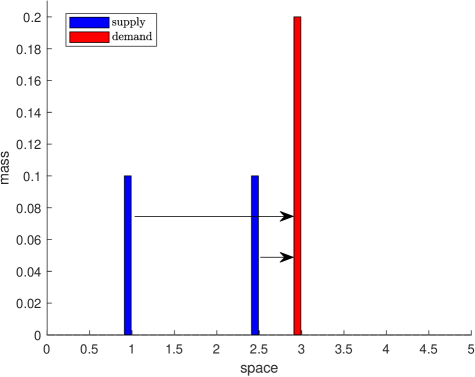
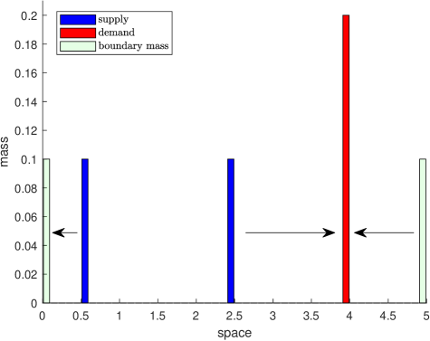
Figure 5: Test 1. Case 1.1 where boundaries are not used (left), and Case 1.2 where mass is both taken from and brought to boundaries (right).

Test 2

In this test we consider the case of continuous unbalanced distributions in the domain $X=[-5,5]$,

$$\rho^{\textsc{s}}(x)=e^{-x^{2}},\qquad\rho^{\textsc{d}}(x)=\frac{e^{-(x-3)^{2}}}{4},$$

see Fig. 6. We set $N=50$ so that $\Delta x=0.2$.

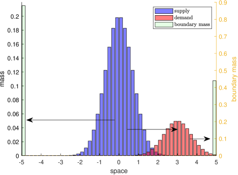
Figure 6: Test 2. Some supply (resp., demand) mass is brought to left (resp., right) boundary, the rest is transported.

In this case the optimal mass transport map prescribes to move a part of the supply mass to the let boundary and a part of the demand mass to the right boundary, then transport the remaining mass. We have $\tilde{W}^{\textsc{fg}}=6.84$.

4.2 Piccoli & Rossi approach

Test 1

Consider the simple example proposed in [19, Sect. 2.2], where authors consider the two constant distributions

$$\rho^{\textsc{s}}(x)=\chi_{[-1,0]}(x),\qquad\rho^{\textsc{d}}(x)=\chi_{[\xi,1+\xi]}(x),\qquad x\in\mathbb{R}$$

with parameter $\xi\geq 0$. The exact value of the GWD (with $a=b=p=1$) is easily computed and gives

$$W^{\textsc{pr}}_{1}(\rho^{\textsc{s}},\rho^{\textsc{d}};1,1)=\left\{\begin{array}[]{ll}1+\xi-\xi^{2}/4,&\text{if }\xi\in[0,2],\\ 2,&\text{if }\xi\geq 2.\end{array}\right.$$

Fig. 7 shows the result of the numerical computation in the domain $X=[-2,5]$ divided in $N=200$ cells, for $\xi\in[0,3]$.

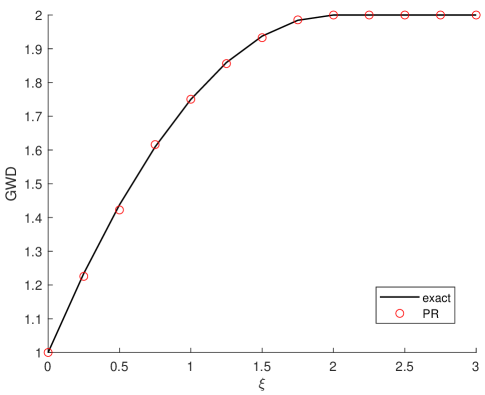
Figure 7: Test 1. Exact solution compared with numerical solution ($N=200$).

Test 2

In this test we run the algorithm in a nontrivial case where exact solution is not known. More in detail, we consider $X=[-4,4]$, $N=100$, $a=b=p=1$, and

$$\rho^{\textsc{s}}(x)=\frac{e^{-x+1}}{5}\chi_{[-2,0]}(x),\qquad\rho^{\textsc{d}}(x)=e^{-(x-1)^{2}}.$$

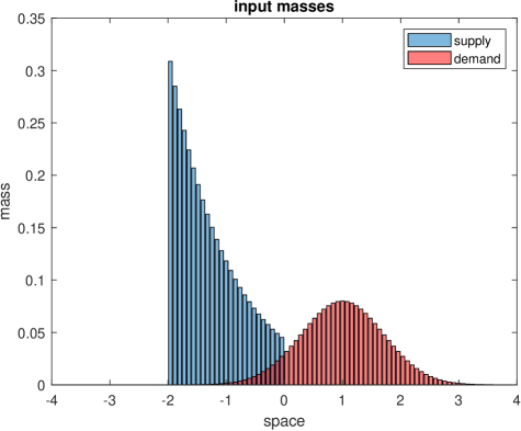
Figure 8: Test 2. Initial distributions $m^{\textsc{s}}$ and $m^{\textsc{d}}$ (left) and remaining masses $\mathring{m}^{\textsc{s}}$ and $\mathring{m}^{\textsc{d}}$ corresponding to the optimal solution (right).

Fig. 8 shows the result in terms of remaining mass after minimization. One can see that here the optimal solution ($\tilde{W}^{\textsc{pr}}_{1}=4.36$) requires to destroy only a part of the mass.

4.3 Gaussian Hellinger–Kantorovich and Savaré & Sodini approaches

As far as we know, this paper is the first one which proposes a practical computation of the GWDs described in Sects. 3.3 and 3.4. We recall here that the two approaches, although quite different from the computational point of view, are theoretically equivalent (with $a=b=1$, which will be always the case from now on). This is also confirmed by our numerical experiments.

Test 1

This test is mainly conceived to check the correctness of the code on simple examples with known exact solution. Let us consider the simplest possible scenario, with only one concentrated supply mass $\delta^{\textsc{s}}$ and only one concentrated demand mass $\delta^{\textsc{d}}$. To simplify the notations, we denote by $m^{\textsc{s}}$, $x^{\textsc{s}}$ and by $m^{\textsc{d}}$, $x^{\textsc{d}}$ the mass and the position of the supply mass and the demand mass, respectively. In this case the exact solution is $\tilde{W}^{\textsc{ghk}}_{2}=\tilde{W}^{\textsc{ss}}_{2}=H_{g}(x^{\textsc{s}},m^{\textsc{s}};x^{\textsc{d}},m^{\textsc{d}})$, where $H_{g}$ is defined in (3.14).

Fig. 9 shows the results of the algorithm for $\tilde{W}^{\textsc{ghk}}_{2}$ as well as both algorithms for $\tilde{W}^{\textsc{ss}}_{2}$ (SS-A and SS-B), alongside the exact solution. More in detail, Fig. 9(left) shows the GWD in the case the two distributions are balanced ($m^{\textsc{s}}=m^{\textsc{d}}=\bar{m}$) and their distance progressively increases from 0 to 6. One can see that the GWD rapidly saturates at $2\bar{m}$.

Fig. 9(right) shows instead the GWD in the case the two distributions are located at the same point and the difference of their masses progressively increases from 0 to 7.

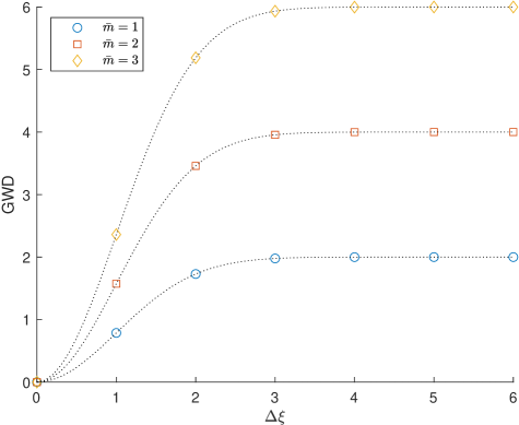
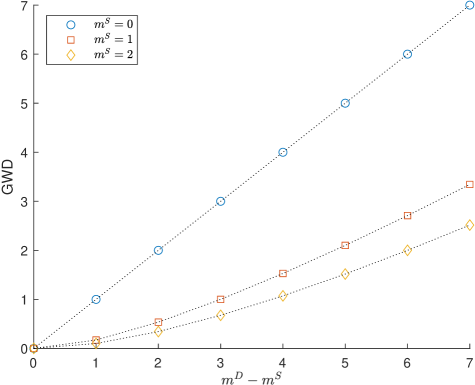
Figure 9: Test 1. GWD between two equal atomic mass distributions with mass $\bar{m}$ as a function of their distance $\Delta\xi$ (left), and GWD between two overlapping atomic mass distributions as a function of the difference of mass (right). Dotted black line is the exact solution.

Test 2

The goal of this test is mainly comparing the algorithms SS-A and SS-B. We consider another simple scenario with only two concentrated masses for supply, and only one concentrated mass for demand, see Fig. 10.

Figure 10: Test 2: two concentrated masses for supply mass and one for demand mass.

We assume that supply masses are located at $x=0$ and $x=1$, have masses $m=2$ and $m=1$, and have $n=2$, $n=1$ additional divisions, respectively. Demand mass is instead located at $x=3$, has mass $m=4$, and has $n=4$ additional divisions. In this scenario it results $d=12$.

Fig. 11(top) shows the history of all the evaluations of $\tilde{W}^{\textsc{ss}}_{2}$ done by the exhaustive algorithm SS-A, in the same order as they are computed, with $Q=6$. One can observe a recursive pattern due to the way $\Gamma$’s are generated (Step 2). Minimum is already found among the first evaluations and it is $\tilde{W}^{\textsc{ss}}_{2}=6.45$.

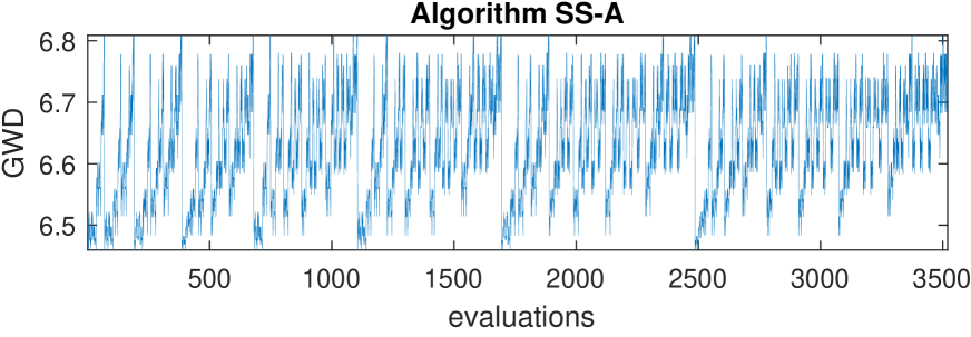
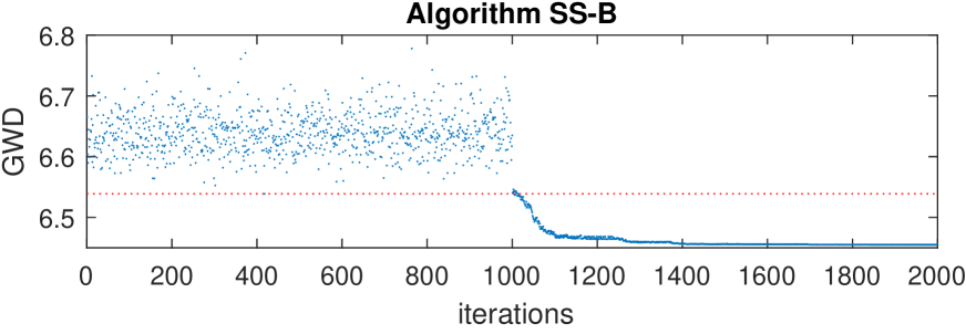
Figure 11: Test 2. Algorithm SS-A, complete view of all the evaluations of $\tilde{W}^{\textsc{ss}}_{2}$ (top), and Algorithm SS-B, 1,000 random searches followed by about 1,000 descend iterations (bottom). Dotted red line indicates the minimum value found in the first phase of SS-B.

Fig. 11(bottom) shows the tentative values of $\tilde{W}^{\textsc{ss}}_{2}$ found in the first exploratory phase of the algorithm SS-B (Steps 1-3), followed by the minimum values found during the random descend, with $Q=1,\!000$. The algorithm returns again $\tilde{W}^{\textsc{ss}}_{2}=6.45$. Convergence seems to be well guaranteed and the two algorithms give the same value for $\tilde{W}^{\textsc{ss}}_{2}$ ($\tilde{W}^{\textsc{ghk}}_{2}$ is also the same).

For these reasons, in the following we will use algorithm SS-B only, which is obviously faster.

4.4 Comparison of the three GWDs

The aim of this section is to compare the four computational approaches for the three GWDs individually studied above, in order to understand which one is the most suitable in the context of traffic flow modeling. This is done by devising a numerical test which can be run by all algorithms. From now on, the four algorithms will be referred to by FG, PR, SS (variant B only), and GHK, with obvious meaning.

Denoting by $\chi$ the indicator function, we consider the case of two time-dependent distributions with parameters $\alpha,\beta,\eta>0$,

$$\rho^{\textsc{s}}(x,t)=\alpha\chi_{\left[-t-\eta,-t+\eta\right]}(x),\qquad\rho^{\textsc{d}}(x,t)=\beta\chi_{\left[t-\eta,t+\eta\right]}(x),\qquad 0\leq t\leq T$$ (4.1)

in the domain $X=[-T-\eta,T+\eta]$. The two step functions start with perfectly overlapping support, then supply mass moves leftward while demand mass moves rightward, until they both reach the boundary of the domain, see Fig. 12.

Figure 12: Moving distributions $\rho^{\textsc{s}}$ and $\rho^{\textsc{d}}$ as defined in (4.1).

In particular, for this comparison test we set $\alpha\in\{1,2\}$, $\beta=2$, $\eta=1$, $T=4$. Moreover, we have the following algorithm-specific parameters:

• PR: $a=2.5$, $b=1$.

• GHK: $a=b=1$.

• SS: $a=b=1$, 4 atomic masses per distribution, 4 additional divisions per mass, $Q=1,\!000$, $\epsilon=0.001$, iterations 5,000 (random searches) + 40,000 (random descend), average on 10 runs.

Fig. 13 shows the behavior of the three GWDs between $\rho^{\textsc{s}}$ and $\rho^{\textsc{d}}$ as defined in (4.1), as a function of time. WD is also shown in the balanced case $\alpha=\beta$.

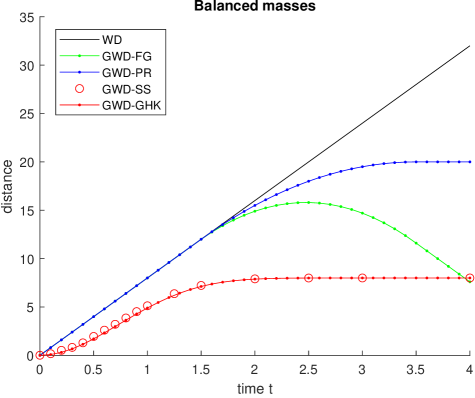
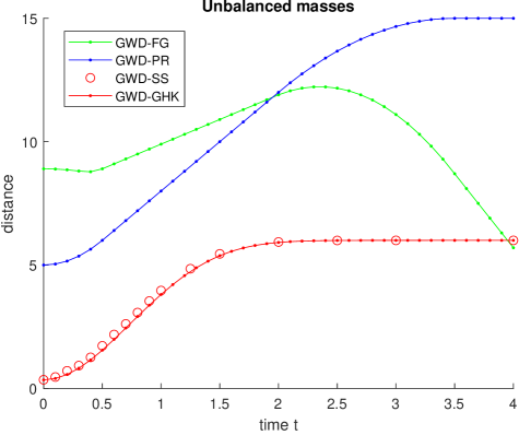
Figure 13: Comparison of the three GWDs between $\rho^{\textsc{s}}$ and $\rho^{\textsc{d}}$ as defined in (4.1), as a function of time $t$ ($\beta=2$, $\eta=1$, $T=4$). $\alpha=2$ (balanced), including also classical WD (left), and $\alpha=1$ (unbalanced, right).

Some preliminary comments

The comparison test (Fig. 13) allows us to sketch some preliminary conclusions. First of all, SS seems to be computationally unfeasible. It is impossible to deal with a reasonable number of concentrated masses and additional divisions.

Among the others, PR and GHK share with $L^{p}$ an important drawback: the distances saturate when distributions do not overlap and they are far enough from each other. This does not seem to be a nice feature in the context of traffic flow models.

Lastly, FG has an important feature which deserves a discussion: the distance decreases whenever distributions are close to the boundaries, even if they are very far from each other. On first glance, this seems to be an issue, but it can be also be seen as a good point: basically, it implies that what happens near the boundaries is less important than what happens on the rest of the road. Considering the fact that boundary conditions are typically unknown in traffic flow modeling, it could make sense to give priority to that part of the road which is less or not at all influenced by boundary conditions.

5 Applications to traffic model analysis

In this section we will try to understand to what extent the GWDs previously studied are suitable in the context of traffic flow models. It is useful to recall here that in [3] authors have already extensively studied the sensitivity of the LWR model [16, 21] using the WD. More precisely, many simulations were performed varying some key parameters like the initial vehicle density, the road capacity (maximal flux), the critical density (vehicle density associated to the maximal flux), the size of the road network, and the distribution coefficients at junctions (how traffic distributes across a junction with more than one outgoing road). Interestingly, authors found that the parameter the model is most sensitive to is the last one, namely the distribution coefficients at junctions. That said, the usage of WD have limited the authors to the comparison of balanced vehicle distributions only. This means, in practice, that the number of vehicles should be the same in the two considered scenarios.

In the following we try to complete the sensitivity analysis including the cases in which the mass distributions are unbalanced. As already mentioned, SS has computational difficulties and will be discarded in the following analysis.

5.1 Mathematical modelling

In a macroscopic setting, traffic flow is described by means of average quantities only, like density $\rho$ (vehicles per unit of space, at a given time), flux $f$ (vehicles per unit of time crossing a given point, at a given time), and velocity $v$. Models can be first-order (i.e., velocity based), if velocity is given as a function of the density and acceleration is neglected, or second-order (i.e., acceleration based) if, instead, velocity is an independent variable and acceleration is given as a function of both density and velocity.

In the following we will assume the road is a finite segment $X=[x_{\textsc{min}},x_{\textsc{max}}]$ with a single lane and a single class of vehicles.

LWR model

The LWR model, introduced independently by Lighthill & Whitham [16] and by Richards [21], describes the evolution of the vehicle density $\rho(x,t)$ by means of the following IBVP involving an hyberbolic PDE

$$\left\{\begin{array}[]{ll}\partial_{t}\rho+\partial_{x}f(\rho)=0,&t\in[t_{0},T],\quad x\in[x_{\textsc{min}},x_{\textsc{max}}],\\ \rho(x,0)=\rho_{0}(x),&x\in[x_{\textsc{min}},x_{\textsc{max}}],\\ \rho(x_{\textsc{min}},t)=\rho_{\textsc{in}}(t),&t\in[t_{0},T],\\ \rho(x_{\textsc{max}},t)=\rho_{\textsc{out}}(t),&t\in[t_{0},T],\end{array}\right.$$ (5.1)

for some initial time $t_{0}$, final time $T>t_{0}$, and concave flux function $f:[0,\rho_{\textsc{max}}]\to\mathbb{R}^{+}$ (called fundamental diagram in the context of traffic flow) such that $f(0)=f(\rho_{\textsc{max}})=0$, for some maximal density $\rho_{\textsc{max}}$. Note that we have naturally guaranteed the constraint $0\leq\rho\leq\rho_{\textsc{max}}$ at any time, provided $0\leq\rho_{0},\rho_{\textsc{in}},\rho_{\textsc{out}}\leq\rho_{\textsc{max}}$.

Recalling the well known physical law $f=\rho v$, which is always valid for any $x$ and $t$, we get that the LWR model implicitly assumes that the vehicle velocity $v$ only depends on the density $\rho$ (since $f=f(\rho)$, therefore $v=v(\rho)$). From the modeling point of view, this means that the velocity adapts instantaneously to the changes of the density, i.e.  acceleration is infinite. For this reason the LWR model is said to be first-order.

As usual in the mathematical literature, in the following we will define

$$f(\rho)=1-\rho,$$

implicitly assuming that the maximal density $\rho_{\textsc{max}}$ and the maximal velocity of vehicles are normalized and equal to 1. This is done for simplicity, since a qualitative analysis is sufficient to highlight the differences among the GWDs.

Eq. (5.1) can be numerically approximated by means of, e.g., the Godunov scheme. Using again the numerical setting introduced in Sect. 2.3, this scheme reads as

$$\rho_{i}^{n+1}=\rho_{i}^{n}-\frac{\Delta x}{\Delta t}\Big{(}\mathcal{G}(\rho_{i}^{n},\rho_{i+1}^{n})-\mathcal{G}(\rho_{i-1}^{n},\rho_{i}^{n})\Big{)},\qquad i=2,\ldots,N-1,\quad n=0,\ldots,\left[\frac{T-t_{0}}{\Delta t}\right],$$ (5.2)

where $\rho_{i}^{n}$ represents the approximated value of $\rho$ at the center of the cell $C_{i}$ at time $t_{0}+n\Delta t$, and $\mathcal{G}$ is the Godunov’s numerical flux defined by

$$\mathcal{G}(\rho_{-},\rho_{+}):=\left\{\begin{array}[]{ll}\displaystyle\min_{z\in[\rho_{-},\rho_{+}]}f(z),&\textrm{if }\rho_{-}\leq\rho_{+},\\[8.53581pt] \displaystyle\max_{z\in[\rho_{+},\rho_{-}]}f(z),&\textrm{if }\rho_{-}\geq\rho_{+}.\\ \end{array}\right.$$ (5.3)

Remark 6.

Boundary conditions can be also given in form of incoming and outgoing flux, rather than as left and right densities $\rho_{\textsc{in}}$, $\rho_{\textsc{out}}$. This happens, e.g., if boundary data are given by fixed sensors counting vehicles passing through $x=x_{\textsc{min}}$ and $x=x_{\textsc{max}}$ in a time interval $\Delta t$. If this is the case, values $\rho_{1}^{n}=\rho_{\textsc{in}}^{n}$ and $\rho_{N}^{n}=\rho_{\textsc{out}}^{n}$ are dropped, and incoming/outgoing fluxes $F_{\textsc{in}}^{n}$, $F_{\textsc{out}}^{n}$ are directly injected in the scheme (5.2) taking the place of $\mathcal{G}(\rho_{i-1}^{n},\rho_{i}^{n})$ if $i=1$, and of $\mathcal{G}(\rho_{i}^{n},\rho_{i+1}^{n})$ if $i=N$, respectively.

ARZ model

The ARZ model, introduced independently by Aw & Rascle [1] and by Zhang [27], describes the evolution of the vehicle density $\rho(x,t)$ and the velocity $v(x,t)$ by means of the following IBVP involving two hyberbolic PDEs

$$\left\{\begin{array}[]{ll}\partial_{t}\rho+\partial_{x}(\rho v)=0,&t\in[t_{0},T],\quad x\in[x_{\textsc{min}},x_{\textsc{max}}],\\ \partial_{t}(\rho w)+\partial_{x}(v\rho w)=\rho\frac{v_{eq}(\rho)-v}{\tau},&t\in[t_{0},T],\quad x\in[x_{\textsc{min}},x_{\textsc{max}}],\\ \rho(x,0)=\rho_{0}(x),&x\in[x_{\textsc{min}},x_{\textsc{max}}],\\ v(x,0)=v_{0}(x),&x\in[x_{\textsc{min}},x_{\textsc{max}}],\\ \rho(x_{\textsc{min}},t)=\rho_{\textsc{in}}(t),&t\in[t_{0},T],\\ \rho(x_{\textsc{max}},t)=\rho_{\textsc{out}}(t),&t\in[t_{0},T],\\ v(x_{\textsc{min}},t)=v_{\textsc{in}}(t),&t\in[t_{0},T],\\ v(x_{\textsc{max}},t)=v_{\textsc{out}}(t),&t\in[t_{0},T],\end{array}\right.$$ (5.4)

where $w(x,t):=v(x,t)+P(\rho(x,t))$, $P(\rho):=\frac{v_{ref}}{\gamma}\left(\frac{\rho}{\rho_{\textsc{max}}}\right)^{\gamma},$ and $v_{ref}$, $\gamma$, an $\tau$ are strictly positive parameters. This time, the velocity $v$ is an independent unknown and the acceleration $\frac{v_{eq}(\rho)-v}{\tau}$ appears explicitly in the model, depending on $\rho$ and $v$. For this reason, the ARZ model is said to be second-order.

In order to fairly compare the two models we define $v_{eq}(\rho):=\frac{f(\rho)}{\rho}$, so that the desired equilibrium velocity of the ARZ model coincides with the instantaneous velocity of the LWR model. Also in the boundary conditions, we set $v_{\textsc{in}}=v_{eq}(\rho_{\textsc{in}})$ and $v_{\textsc{out}}=v_{eq}(\rho_{\textsc{out}})$.

Eq. (5.4) is numerically approximated by means of the Lax–Friedrichs scheme.

5.2 Numerical tests

5.2.1 Test 1: sensitivity to boundary conditions

In this test we investigate the sensitivity to boundary conditions. We consider the case described in Rem. 6, which is a scenario often met in real life [4]. In the same spirit of [4], we assume that the time interval is divided in two subintervals: $[t_{0},0]$ and $(0,T]$, where $t=0$ corresponds to the current time (the ‘now’), i.e. the time the simulation is actually performed. Until time 0, we can rely on the sensors’ measurements $F_{\textsc{in}}$, $F_{\textsc{out}}$, and we use it as boundary conditions (see Rem. 6). After that time, we have no such a data because they are not yet available, but we assume to be able to (exactly) forecast the average value of them,

$$\hat{F}_{\textsc{in}}=\frac{1}{T}\int_{0}^{T}F_{\textsc{in}}(t)dt,\qquad\hat{F}_{\textsc{out}}=\frac{1}{T}\int_{0}^{T}F_{\textsc{out}}(t)dt.$$

In short: we denote by $\rho^{\textsc{s}}$ the “exact” solution obtained by using boundary fluxes $F_{\textsc{in}}(t)$, $F_{\textsc{out}}(t)$ in the whole interval $[t_{0},T]$, and by $\rho^{\textsc{d}}$ the “predicted” solution obtained by using flux boundary data $F_{\textsc{in}}(t)$, $F_{\textsc{out}}(t)$ until time $t=0$ and then by using the predicted average values $\hat{F}_{\textsc{in}}$, $\hat{F}_{\textsc{out}}$ until time $T$. At any time $t$, the vehicle distributions $\rho^{\textsc{s}}(\cdot,t)$ and $\rho^{\textsc{d}}(\cdot,t)$ are compared computing the GWDs.

Initial conditions are $\rho^{\textsc{s}}(x,t_{0})=\rho^{\textsc{d}}(x,t_{0})=0.2$ for any $x$. Boundary fluxes are randomly generated: $F_{\textsc{in}}$ has uniform distribution in $[0,\frac{1}{4}]$, $F_{\textsc{out}}$ has uniform distribution in $[0,\mathcal{G}(0.2,0.2)]$. Other parameters are: $x_{\textsc{min}}=0$, $x_{\textsc{max}}=40$, $t_{0}=-10$, $T=30$, $\Delta x=0.4$ (corresponding to $N=100$), and $\Delta t=0.25$.

Fig. 14 shows two screenshots of the simulations at times $t=0$ and $t=12$.

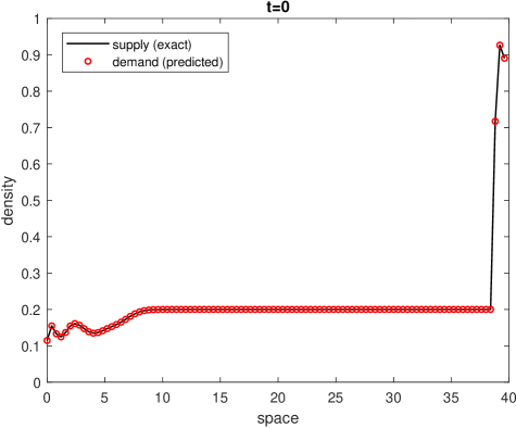
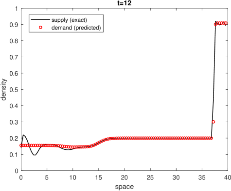
Figure 14: Test 1 on sensitivity to boundary conditions. Two screenshots at $t=0$ (‘now’), i.e. when solutions cease to be equal (left), and $t=12$ (right).

Fig. 15 shows the total mass on the road and the GWDs between $\rho^{\textsc{s}}(\cdot,t)$ and $\rho^{\textsc{d}}(\cdot,t)$ at any time.

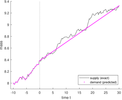
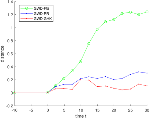
Figure 15: Test 1 on sensitivity to boundary conditions. Difference of mass between the two simulations (left) and comparison of GWDs (right).

5.2.2 Test 2: sensitivity to traffic light cycle

In this test we consider a shorter road with respect to the previous test, and we assume there is a traffic light in the middle of the road, at the interface between two numerical cells. The duration of the red phase equals that of the green phase. Technically, the red traffic light is modeled by imposing null flux at the right (resp., left) boundary of the cell before (resp., after) the traffic light. The aim is to investigate the sensitivity to the duration of the traffic light cycle.

Initial conditions are $\rho^{\textsc{s}}(x,t_{0})=\rho^{\textsc{d}}(x,t_{0})=0$ for any $x$. Left Dirichlet boundary conditions are $\rho_{\textsc{in}}^{\textsc{s}}=\rho_{\textsc{in}}^{\textsc{d}}=0.4$. Right Dirichlet boundary conditions are $\rho_{\textsc{out}}^{\textsc{s}}=\rho_{\textsc{out}}^{\textsc{d}}=0$. Other parameters are: $x_{\textsc{min}}=0$, $x_{\textsc{max}}=4$, $t_{0}=0$, $T=20$, $\Delta x=0.04$ (corresponding to $N=100$), and $\Delta t=0.025$. Both red and green phases last 50 time steps for supply distribution and 40 time steps for demand distribution.

Fig. 16 shows two screenshots of the simulations at times $t=3.7$ and $t=7.4$.

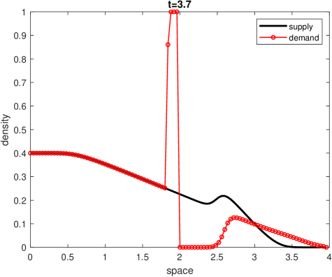
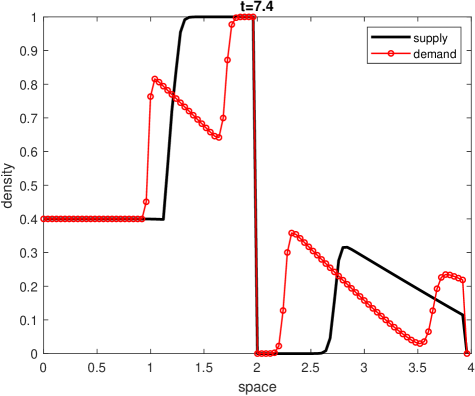
Figure 16: Test 2 on sensitivity to traffic light cycle. Two screenshots at $t=3.7$ with red traffic light for demand and green traffic light for supply (left), and $t=7.4$ with red traffic light for both distributions (right).

Fig. 17 shows the total mass on the road in the two scenarios and the GWDs between $\rho^{\textsc{s}}(\cdot,t)$ and $\rho^{\textsc{d}}(\cdot,t)$ at any time.

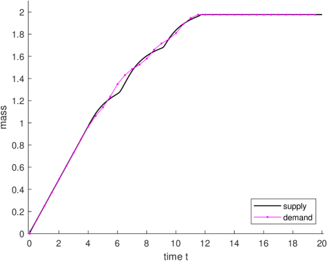
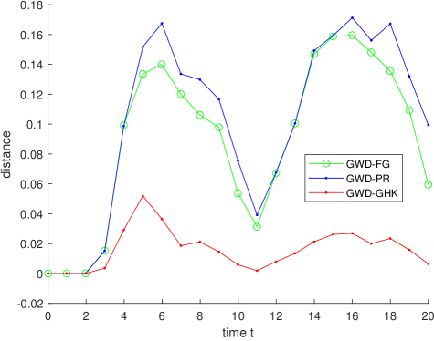
Figure 17: Test 2 on sensitivity to traffic light cycle. Difference of mass between the two simulations (correctly masses differ only in a certain time interval, left), and comparison of GWDs (right).

5.2.3 Test 3: sensitivity to model order

In this test we quantify the difference between two simulations obtained by means of the LWR model (supply, first-order) and the ARZ model (demand, second-order).

Initial conditions are $\rho^{\textsc{s}}(x,t_{0})=\rho^{\textsc{d}}(x,t_{0})=0.7$ for $x\in[1.6,2.4]$ and 0.1 elsewhere. Left and right Dirichlet boundary conditions are null. Other parameters are: $\tau=0.05$, $\gamma=2$, $v_{ref}=1$, $x_{\textsc{min}}=0$, $x_{\textsc{max}}=4$, $t_{0}=0$, $T=3$, $\Delta x=0.02$ (corresponding to $N=200$), and $\Delta t=0.01$.

Fig. 18 shows two screenshots of the simulations at times $t=0.3$ and $t=1$.

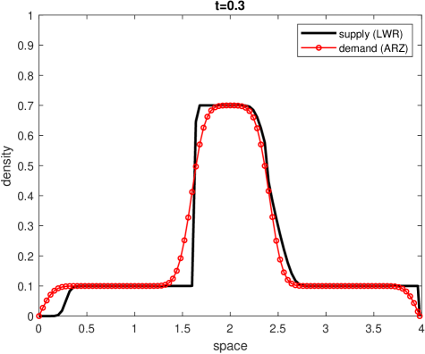
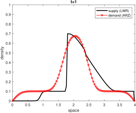
Figure 18: Test 3 on sensitivity to model order. Two screenshots at $t=0.3$ (left), and $t=1$ (right).

Fig. 19 shows the total mass on the road in the two scenarios and the GWDs between $\rho^{\textsc{s}}(\cdot,t)$ and $\rho^{\textsc{d}}(\cdot,t)$ at any time. Here we have chosen $a=0.5$ and $b=1$ as parameters for computing $\tilde{W}^{\textsc{pr}}_{1}$.

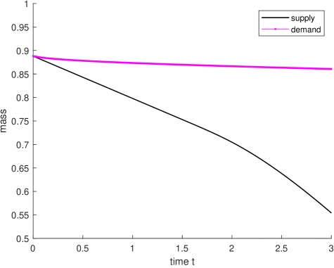
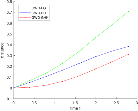
Figure 19: Test 3 on sensitivity to model order. Difference of mass between the two simulations (left) and comparison of GWDs (right).

Comments and conclusions

Observing the results of the last numerical tests, we tend to confirm what we have anticipated in Sect. 4.4, namely that the Figalli & Gigli approach seems to be the most suitable GWD to be used in the context of traffic flow modeling, mainly because of how boundaries are regarded.

In this respect, the most significant test is probably the first one, in Sect. 5.2.1: here the discrepancy between the exact and predicted solution slowly propagates from the boundaries to the interior of the road, impacting more and more on the reliability of the traffic prediction. This behavior of the error is clearly better caught by FG (see Fig. 17-right), which is the last distance that saturates.

Although less evident, the same conclusions apply for the third test, in Sect. 5.2.3: here the two solutions start differing immediately, both at the boundary and inside the road. Moreover, the difference increases as the time goes by. Among the three GWDs, FG is the one which increases more rapidly at the initial time, and then keeps increasing all the time.

Conversely, the second test does not show much difference among the three GWDs, having them basically the same cycling behavior. That behavior is correct since the two solutions cyclically move away from each other and then come closer again.

Overall, we have proposed four algorithms for computing, in a discrete context, four GWDs (two of them theoretically equivalent to each other). One of them (SS) results to be numerically unfeasible, while the other three (namely FG, PR, GHK) are all relative simple to implement once the computational procedure is arranged.

In a future work, we will aim at exploring the possibility to compute the considered GWDs in more complicated domain like $\mathbb{R}^{2}$, $\mathbb{R}^{3}$, and (road) networks.

Funding.

M.B. and E.C. would like to thank the Italian Ministry of University and Research (MUR) to support this research with funds coming from PRIN Project 2022 PNRR entitled “Heterogeneity on the road - Modeling, analysis, control”, No. 2022XJ9SX.

E.C. would like to thank the Italian Ministry of University and Research (MUR) to support this research with funds coming from PRIN Project 2022 entitled “Optimal control problems: analysis, approximation and applications”, No. 2022238YY5.

G.F. would like to thank the Italian Ministry of University and Research (MUR) to support this research with funds coming from PRIN Project 2022 entitled “Variational analysis of complex systems in materials science, physics and biology”, No. 2022HKBF5C, CUP B53D23009290006.

This study was carried out within the Spoke 7 of the MOST – Sustainable Mobility National Research Center and received funding from the European Union Next-Generation EU (PIANO NAZIONALE DI RIPRESA E RESILIENZA (PNRR) – MISSIONE 4 COMPONENTE 2, INVESTIMENTO 1.4 – D.D. 1033 17/06/2022, CN00000023).

This manuscript reflects only the authors’ views and opinions. Neither the European Union nor the European Commission can be considered responsible for them.

E.C. and F.L.I. are funded by INdAM–GNCS Project, CUP E53C23001670001, entitled “Numerical modeling and high-performance computing approaches for multiscale models of complex systems”.

M.B., E.C., and F.L.I. are members of the e INdAM research group GNCS, while G.F. is member of the e INdAM research group GNAMPA.

Acknowledgments.

Authors want to thank Benedetto Piccoli, Francesco Rossi, Giuseppe Savaré, and Giacomo Enrico Sodini for the useful discussions, and Anna Thünen for the contribution given to Sect. 3.1.2.

References

- [1] A. Aw and M. Rascle. Resurrection of “second order” models of traffic flow? SIAM J. Appl. Math., 60:916–938, 2000.
- [2] J.-D. Benamou and Y. Brenier. A computational fluid mechanics solutions to the Monge–Kantoriovich mass transfer problem. Numer. Math., 84(3):375–393, 2000.
- [3] M. Briani, E. Cristiani, and E. Iacomini. Sensitivity analysis of the LWR model for traffic forecast on large networks using Wasserstein distance. Commun. Math. Sci., 16(1):123–144, 2018.
- [4] M. Briani, E. Cristiani, and E. Onofri. Inverting the fundamental diagram and forecasting boundary conditions: How Machine Learning can improve macroscopic models for traffic flow. To appear on Advances in Computational Mathematics. Preprint arXiv:2303.12740.
- [5] L. Caffarelli and R. J. McCann. Free boundaries in optimal transport and Monge-Ampère obstacle problems. Annals of Mathematics, 171(2):673–730, 2010.
- [6] L. Chizat, G. Peyré, B. Schmitzer, and F.-X. Vialard. An interpolating distance between optimal transport and Fisher-Rao metrics. Foundation of Computational Mathematics, 18:1–44, 2018.
- [7] L. Chizat, G. Peyré, B. Schmitzer, and F.-X. Vialard. Unbalanced optimal transport: Dynamic and Kantorovich formulations. Journal of Functional Analysis, 274:3090–3123, 2018.
- [8] E. Cristiani, B. Piccoli, and A. Tosin. Multiscale modeling of pedestrian dynamics, volume 12 of Series Modeling, Simulation & Applications. Springer, 2014.
- [9] E. Cristiani and M. C. Saladino. Comparing comparisons between vehicular traffic states in microscopic and macroscopic first-order models. Mathematical Methods in the Applied Sciences, 42(3):918–934, 2019.
- [10] A. Figalli. The optimal partial transport problem. Archive for Rational Mechanics and Analysis, 195(2):533–560, 2010.
- [11] A. Figalli and N. Gigli. A new transportation distance between non-negative measures, with applications to gradients flows with Dirichlet boundary conditions. Journal de Mathématiques Pures et Appliquées, 94(2):107–130, 2010.
- [12] L. G. Hanin. Kantorovich-Rubinstein norm and its application in the theory of Lipschitz spaces. Proceedings of the American Mathematical Society, 115(2):345–352, 1992.
- [13] L. Kantorovich and G. S. Rubinstein. On a space of totally additive functions. Vestnik Leningradskogo Universiteta, 13:52–59, 1958.
- [14] S. Kondratyev, L. Monsaingeon, and D. Vortnikov. A new optimal transport distance on the space of finite Radon measures. Adv. Differential Equations, 21(11/12):1117–1164, 2016.
- [15] M. Liero, A. Mielke, and G. Savaré. Optimal entropy-transport problems and a new Hellinger-Kantorovich distance between positive measures. Invent. Math., 211(3):969–1117, 2018.
- [16] M. J. Lighthill and G. B. Whitham. On kinematic waves II. A theory of traffic flow on long crowded roads. Proc. R. Soc. Lond. Ser. A, 229:317–345, 1955.
- [17] L. Lombardini and F. Rossi. Obstructions to extension of Wasserstein distances for variable masses. Proceedings of the American Mathematical Society, 150(11):4879–4890, 2022.
- [18] Z. Ma, X. Wei, X. Hong, H. Lin, Y. Qiu, and Y. Gong. Learning to count via unbalanced optimal transport. In Proceedings of the AAAI Conference on Artificial Intelligence, volume 35, pages 2319–2327, 2021.
- [19] B. Piccoli and F. Rossi. Generalized Wasserstein distance and its application to transport equations with source. Archive for Rational Mechanics and Analysis, 211:335–358, 2014.
- [20] B. Piccoli and F. Rossi. On properties of the generalized Wasserstein distance. Arch. Rational Mech. Anal., 222:1339–1365, 2016.
- [21] P. I. Richards. Shock waves on the highway. Oper. Res., 4:42–51, 1956.
- [22] F. Santambrogio. Optimal Transport for Applied Mathematicians. Calculus of Variations, PDEs, and Modeling, volume 87 of Series Progress in Nonlinear Differential Equations and Their Applications. Birkhäuser, 2015.
- [23] G. Savaré and G. E. Sodini. A relaxation viewpoint to Unbalanced Optimal Transport: Duality, optimality and Monge formulation. Journal de Mathématiques Pures et Appliquées, 188:114–178, 2024.
- [24] S. M. Sinha. Mathematical Programming. Theory and Methods. Elsevier, 2006.
- [25] C. Villani. Topics in Optimal Transportation, volume 58 of Series Graduate Studies in Mathematics. American Mathematical Society, 2003.
- [26] C. Villani. Optimal Transport. Old and New, volume 338 of Series Grundlehren der mathematischen Wissenschaften. Springer, 2009.
- [27] H. M. Zhang. A non-equilibrium traffic model devoid of gas-like behavior. Transportation Res. Part B, 36:275–290, 2002.