A Simple Approach to Unifying Diffusion-based Conditional Generation

Abstract

Recent progress in image generation has sparked research into controlling these models through condition signals, with various methods addressing specific challenges in conditional generation. Instead of proposing another specialized technique, we introduce a simple, unified framework to handle diverse conditional generation tasks involving a specific image-condition correlation. By learning a joint distribution over a correlated image pair (e.g. image and depth) with a diffusion model, our approach enables versatile capabilities via different inference-time sampling schemes, including controllable image generation (e.g. depth to image), estimation (e.g. image to depth), signal guidance, joint generation (image & depth), and coarse control. Previous attempts at unification often introduce significant complexity through multi-stage training, architectural modification, or increased parameter counts. In contrast, our simple formulation requires a single, computationally efficient training stage, maintains the standard model input, and adds minimal learned parameters (15% of the base model). Moreover, our model supports additional capabilities like non-spatially aligned and coarse conditioning. Extensive results show that our single model can produce comparable results with specialized methods and better results than prior unified methods. We also demonstrate that multiple models can be effectively combined for multi-signal conditional generation.

1 Introduction

Text-to-image diffusion models, such as Dall-E 2 (OpenAI, 2023) and Imagen (Ho et al., 2022a), have revolutionized the field of image generation, leading to contemporary models (Midjourney, 2023; Baldridge et al., 2024) that can produce images almost indistinguishable from real ones. This progress in generative modeling, particularly with diffusion models, has spawned new research areas and reshaped existing fields within computer vision. With advancements in image quality, the generative community has expanded its focus to controllability, resulting in many different approaches, each promoting a distinct scheme for guiding the generative process. ControlNet (Zhang et al., 2023b) highlights the effectiveness of using modalities like depth and edges as conditional input. Meanwhile, other works, such as Loose Control (Bhat et al., 2024) and Readout Guidance (Luo et al., 2024), propose alternative conditioning types (e.g. coarse depth maps) and control mechanisms (e.g. guidance through a prediction head). Concurrently, the estimation community has seen diffusion models advance the state-of-the-art for predicting various modalities from RGB images, e.g. Marigold (Ke et al., 2024) repurposes a pretrained image generator to generate depth instead. In addition, other work Stan et al. (2023) has explored joint diffusion, generating paired image and depth simultaneously.

Although typically addressed as separate tasks within distinct communities, these problems share a common underlying structure: conditional generation between correlated images. Consider the relationship between an image and its depth map: controllable generation translates depth to image, estimation maps image to depth, guidance uses depth predictions to guide image generation, and joint generation produces image-depth pairs. This observation motivates us to unify all these tasks under a global distribution modeling problem. While a few works (Qi et al., 2024; Zhang et al., 2023a) have also explored unified models capable of handling these diverse tasks, they often introduce significant complexity through multi-stage training, increased parameter counts, or architectural modifications. This additional complexity makes creating and using these models difficult, hindering their adoption.

In this paper, we propose UniCon, a unified diffusion model that learns an image-condition joint distribution with a flexible model architecture and simple but effective training strategy to support diverse inference behaviors. We propose an architecture adaptation to the standard image generator diffusion model that is more flexible than ControlNet (allowing for non-pixel-aligned conditioning signals) and more efficient to train, decreasing both the number of learned parameters and required training samples. Inspired by Diffusion Forcing (Chen et al., 2024a), we use a training scheme that disentangles the noise sampling of the image and the condition, allowing flexible sampling strategies at inference time to achieve different conditional generation tasks without explicit mask input.

As shown in Fig. 1, with the same model but different sampling schedules, UniCon can do: 1) controllable image generation in the form of ControlNet, Readout Guidance, and Loose Control, 2) estimation, and 3) joint generation. We train our models based on a large text-to-image model for several different modalities (depth, edges, human poses, image appearance) and show that the behavior of our single model is similar to or better than specialized methods using standard image quality and alignment metrics. We demonstrate significant improvements over prior unified models in conditional generation, training efficiency, and generation flexibility. We also show that UniCon can combine multiple models for multi-signal conditional generation or switch our model to other base model checkpoints. Our models are trained in about 13 hours on 2-4 Nvidia A800 80G GPUs, adding 15% parameters to the base model.

The main contributions of this work are:

• Proposing a framework that unifies controllable generation, estimation, and joint generation, including model adaptation, training strategy, and sampling methods allowing flexible conditional generation at inference.

• Demonstrating that our architecture and training can work on a large-scale text-to-image diffusion model with a small number of learned parameters and a relatively small training data scale.

• Showing that our unified models can perform similar to specialized methods or better than current unified approaches on different modalities.

2 Related Work

Controllable Generation. Fine-tuning text-to-image diffusion models to conditional image generation on signals beyond text has gained significant popularity (Huang et al., 2023; Zhang et al., 2023b; Ye et al., 2023; Mou et al., 2023; Sohn et al., 2023). ControlNet (Zhang et al., 2023b) trains a control network attached to pre-trained diffusion models to incorporate condition signals, such as edge maps, segmentation masks, and pose estimation. Based on ControlNet, LooseControl (Bhat et al., 2024) generalizes depth conditioning to loose depth maps that specify scene boundaries and object positions. Readout-Guidance (Luo et al., 2024) proposes a new control scheme by adding prediction heads to internal features and guiding the generation by the predicted condition signal. Conditional editing tasks, such as DiffEdit  (Couairon et al., 2023), have enhanced conditional image manipulation by applying diffusion-based models for inpainting and editing tasks. Instead of one specific control behavior, our proposed framework provides diverse controlling abilities through different sampling strategies.

Estimation. Extracting signals like depth, surface normals, or segmentation maps from RGB images has been a longstanding challenge in computer vision. Typically, each task has been addressed in isolation or limited combinations,e.g. joint depth and segmentation, but distinct from image generation. Starting works like DDVM (Saxena et al., 2023a), these tasks have started to be addressed directly with diffusion models including depth prediction (Saxena et al., 2023b; a), optical flow prediction (Saxena et al., 2023a), correspondence matching (Nam et al., 2024), etc.. Recently, there has been considerable interest in either using generative features inside estimators (Xu et al., 2023; Zhao et al., 2023) or explicitly fine-tuning image generators as estimators, such as Marigold (Ke et al., 2024) which adds a clean RGB conditioning and fine-tunes the entire model to diffuse a depth map. While Marigold shares some similarities with our depth estimation setting for our RGBD model, our approach differs significantly in both goals and techniques. Unlike Marigold, which focuses solely on depth and discards image generation capabilities, our method retains the ability to perform image generation, depth estimation, and other tasks, through lightweight LoRA fine-tuning.

Joint and Unified Generation. While less common than controllability or estimation, several works have attempted to unify multiple images and modalities within a single model. LDM3D (Stan et al., 2023) jointly generates image and depth data in an RGBD latent space. Following approaches commonly include an inpainting mask in the input to extend joint generation to bidirectional conditional generation. For example, UniGD (Qi et al., 2024) unifies image synthesis and segmentation through a diffusion model trained with image, segmentation, and inpainting mask as inputs. JeDi (Zeng et al., 2024) learns a joint distribution over images that share a common object, facilitating personalized image generation. Among the most relevant works, JointNet (Zhang et al., 2023a) adopts a symmetric ControlNet-like structure for generating both image and depth, utilizing an inpainting scheme to support depth-to-image and image-to-depth generation. Our approach presents several improvements over these unified methods. First, our training strategy enables flexible conditional generation without requiring an explicit mask input. Thus we can avoid concatenating multiple inputs in the feature dimension or adding inpainting masks, which allows our model to act like adapters that can be plugged into the base model checkpoints. Furthermore, our structure supports both loosely correlated image pairs (as in JeDi) and densely correlated pairs (as in JointNet), providing more versatile capabilities across different scenarios.

3 Preliminaries

Diffusion Model. Diffusion models (Sohl-Dickstein et al., 2015; Ho et al., 2020; Song et al., 2020b) are generative models that model a data distribution $p({\mathbf{x}})$ through an iterative denoising process. Consider a forward process gradually adding Gaussian noise $\epsilon$ to data ${\mathbf{x}}_{0}\sim p({\mathbf{x}})$ with timesteps $t=1,\dots,T$ and noise schedule $\{\alpha_{t}\}$,

$$q({\mathbf{x}}_{t}|{\mathbf{x}}_{0})=\mathcal{N}({\mathbf{x}}_{t};\sqrt{\bar{\alpha}_{t}}{\mathbf{x}}_{0},(1-\bar{\alpha}_{t}){\bm{I}}),\quad q({\mathbf{x}}_{t}|{\mathbf{x}}_{t-1})=\mathcal{N}({\mathbf{x}}_{t};\sqrt{\alpha_{t}}{\mathbf{x}}_{t-1},(1-\alpha_{t}){\bm{I}}),$$ (1)

where $\bar{\alpha}_{t}=\prod_{s=1}^{t}\alpha_{s}$ and $x_{T}\sim\mathcal{N}(0,{\bm{I}})$ reaches pure noise. Diffusion models learn to denoise $x_{t}$ at any timestep by estimating $\hat{{\mathbf{x}}}_{\theta}({\mathbf{x}}_{t},t)\approx{\mathbf{x}}_{0}$. According to common $\bm{\epsilon}$-parameterization, we can train the model to predict the noise $\bm{\epsilon}_{\theta}({\mathbf{x}}_{t},t)$ instead using the following least squares objective,

$$\min_{\theta}E_{{\mathbf{x}}_{0},\bm{\epsilon},t}\|\bm{\epsilon}-\bm{\epsilon}_{\theta}({\mathbf{x}}_{t},t)\|^{2},$$ (2)

where ${\mathbf{x}}_{t}=\text{AddNoise}({\mathbf{x}}_{0},t)=\sqrt{\bar{\alpha}_{t}}{\mathbf{x}}_{0}+\sqrt{1-\bar{\alpha}_{t}}\bm{\epsilon}$ and $\bm{\epsilon}\sim\mathcal{N}(0,{\bm{I}})$ is random noise. With the trained denoiser, one can adopt any sampler (Ho et al., 2020; Song et al., 2020a; Karras et al., 2022) to sample new data from noise. Recent latent diffusion models (Rombach et al., 2022; Ramesh et al., 2022) map image data into the latent space to improve performance and efficiency. We base our experiments on Stable Diffusion (Rombach et al., 2022), a large-scale text-to-image latent diffusion model.

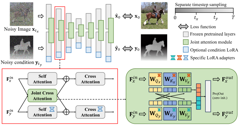
Figure 2: UniCon pipeline. Given a pair of image-condition inputs, our UniCon model processes them concurrently in two parallel branches, with injected joint cross-attention modules where features from two branches attend to each other. We use LoRA weights to adapt our model from a pretrained diffusion model. During training, we separately sample timesteps for each input and compute loss over both branches.

4 Method

Our method, UniCon, aims to train a unified diffusion model for diverse conditional image generation tasks, such as conditional generation on clean, coarse, or partial control signals, estimation, and joint generation. The key idea is to learn a joint distribution over a correlated image pair ${\mathbf{x}},{\mathbf{y}}$, which allows flexible conditional sampling. The image pair can have strict spatial alignment (image-depth, image-edge) or loose semantic correspondence (frames from one video clip). In Sec. 4.1, we first introduce our motivation for learning the joint distribution. Then, we elaborate on our model structure and training pipeline in Sec. 4.2 and the sampling strategies for flexible conditional generation in Sec. 4.3.

4.1 Motivation

Image diffusion models offer significant flexibility when sampling in the learned image distribution $p({\mathbf{x}})$. In addition to generating new image ${\mathbf{x}}\sim p({\mathbf{x}})$, one can perform image inpainting by conditioning partial image ${\mathbf{x}}^{m}$ and image editing by conditioning noisy image ${\mathbf{x}}_{t}$, corresponding to sampling in conditional distributions $p({\mathbf{x}}|{\mathbf{x}}^{m})$ and $p({\mathbf{x}}|{\mathbf{x}}_{t})$. Our motivation is to generalize these abilities from a single image to a correlated image pair $({\mathbf{x}},{\mathbf{y}})$ by learning a joint distribution $p({\mathbf{x}},{\mathbf{y}})$. We then use the modeled joint distribution to enable flexible conditional generation. If the conditional signal is encoded as image ${\mathbf{y}}$, we can train a diffusion model to denoise both image ${\mathbf{x}}$ and condition ${\mathbf{y}}$. The trained joint diffusion model supports various conditional generation tasks that can be unified as sampling in the following conditional distribution,

$$({\mathbf{x}},{\mathbf{y}})\sim p({\mathbf{x}},{\mathbf{y}}|{\mathbf{x}}_{t_{x}}^{m_{x}},{\mathbf{y}}_{t_{y}}^{m_{y}}),$$ (3)

where ${\mathbf{x}}_{t_{x}}^{m_{x}}$ indicates ${\mathbf{x}}$ partially masked by mask $m_{x}$ under noise level (timestep) $t_{x}$.

Sampling in the joint conditional distribution can be regarded as a direct generalization of image inpainting and editing. The conditional generation and estimation are equivalent to inpainting image ${\mathbf{x}}$ or condition ${\mathbf{y}}$ ($p({\mathbf{x}}|{\mathbf{y}}_{0}),p({\mathbf{y}}|{\mathbf{x}}_{0})$). We can also inpaint image and condition for partial control ($p({\mathbf{x}},{\mathbf{y}}|{\mathbf{x}}_{0}^{m_{x}},{\mathbf{y}}_{0}^{m_{y}})$). Adding noise to ${\mathbf{y}}$ enables the model to accept coarse condition input ($p({\mathbf{x}},{\mathbf{y}}|{\mathbf{y}}_{t})$) like SDEdit (Meng et al., 2021) does for image. We can control the condition fidelity by adjusting the noise level. To sum up, combining spatial masking $m_{x},m_{y}$ and noise masking $t_{x},t_{y}$ provides substantial possibilities in free-form conditional generation.

Based on this motivation, our goal is to train a unified diffusion model for targeted image pair $({\mathbf{x}},{\mathbf{y}})$ and develop sampling strategies to support the conditional sampling described in Eq. 3.

4.2 UniCon

Figure 2 illustrates the model structure and training pipeline of the proposed UniCon. Instead of training a new model from scratch, we leverage existing large-scale diffusion models (Rombach et al., 2022) as a starting point. Since these models have learned a strong image prior, it is more efficient to adapt the prior for a single image $p({\mathbf{x}})$ to model the joint distribution of a correlated image pair, $p({\mathbf{x}},{\mathbf{y}})$, than to learn this distribution from scratch.

Given a noisy image pair $({\mathbf{x}}_{t_{x}},{\mathbf{y}}_{t_{y}})$, we feed them as a batch into the denoising network. They are simultaneously processed in two parallel branches, denoted as ${\mathbf{x}}$-branch and ${\mathbf{y}}$-branch. By default, ${\mathbf{x}}$ is the image, and ${\mathbf{y}}$ is the condition. When the conditional image differs from a natural image, we add a LoRA (Hu et al., 2021) to the ${\mathbf{y}}$-branch, which serves to adapt the image generator to produce, e.g. depth or edges. Additional joint cross-attention modules are injected parallel to the self-attention modules to join two branches. During training, we separately sample the timesteps $t_{x},t_{y}$ for ${\mathbf{x}},{\mathbf{y}}$ and optimize the model with the standard diffusion MSE loss from both branches. Next we provide details on our joint cross-attention modules, LoRA adaptation, and training strategy.

Joint cross attention. The joint cross-attention module is the key component that enables ours model to learn a joint distribution $p({\mathbf{x}},{\mathbf{y}})$ given the marginal distributions $p({\mathbf{x}}),p({\mathbf{y}})$. It entangles ${\mathbf{x}}$-branch and ${\mathbf{y}}$-branch with cross branch attention.

The UNet (Ronneberger et al., 2015) is among the most common diffusion model implementation and consists of residual blocks and transformer blocks. As shown in prior work (Tumanyan et al., 2023), the self-attention modules in the transformer blocks are crucial in determining the image structure and appearance. Therefore, we inject the joint cross-attention modules in parallel to the self-attention modules. The module receives the features from both branches as input, with its outputs being added to the self-attention output of the two branches. Specifically, given the input features of two branches $\mathbf{F}_{x}^{\textrm{in}},\mathbf{F}_{y}^{\textrm{in}}$, the output features $\mathbf{F}_{x}^{\textrm{out}},\mathbf{F}_{y}^{\textrm{out}}$ are computed as,

$$\begin{split}&\mathbf{F}_{x}^{\textrm{joint}},\mathbf{F}_{y}^{\textrm{joint}}=\text{JointCrossAttn}(\mathbf{F}_{x}^{\textrm{in}},\mathbf{F}_{y}^{\textrm{in}}),\\ &\mathbf{F}_{x}^{\textrm{out}}=\text{SelfAttn}(\mathbf{F}_{x}^{in})+\mathbf{F}_{x}^{\textrm{joint}},\quad\mathbf{F}_{y}^{\textrm{out}}=\text{SelfAttn}(\mathbf{F}_{y}^{\textrm{in}})+\mathbf{F}_{y}^{\textrm{joint}}.\end{split}$$ (4)

In the joint cross-attention, two features $\mathbf{F}_{x}^{\textrm{in}},\mathbf{F}_{y}^{\textrm{in}}$ attend to each other instead of attending to themselves as in the self-attention. First, features are projected into queries $\mathbf{Q}_{x},\mathbf{Q}_{y}$, keys $\mathbf{K}_{x},\mathbf{K}_{y}$, and values $\mathbf{V}_{x},\mathbf{V}_{y}$. We use different matrices to project ${\mathbf{x}}$ features and ${\mathbf{y}}$ features. For instance, $\mathbf{Q}_{x}=\mathbf{F}_{x}^{in}\mathbf{W}_{Q_{x}},\mathbf{Q}_{y}=\mathbf{F}_{y}^{in}\mathbf{W}_{Q_{y}}$. Then we perform cross-attention between ${\mathbf{x}}$ and ${\mathbf{y}}$ in bidirection,

$$\mathbf{O}_{x}=\text{Softmax}(\frac{\mathbf{Q}_{x}\mathbf{K}_{y}^{T}}{\sqrt{d}})\cdot\mathbf{V}_{y},\quad\mathbf{O}_{y}=\text{Softmax}(\frac{\mathbf{Q}_{y}\mathbf{K}_{x}^{T}}{\sqrt{d}})\cdot\mathbf{V}_{x},$$ (5)

where $d$ is the feature dimension and the feed-forward projection after the attention operation is omitted. Essentially, ${\mathbf{x}}$ aggregates ${\mathbf{y}}$ values $\mathbf{V}_{y}$ according to the query-key similarity matrix $\mathbf{Q}_{x}\mathbf{K}_{y}^{T}$, and vice versa. As a common practice (Zhang et al., 2023b; Guo et al., 2024), we add a zero-initialized linear projection ProjOut at the end to ensure the training starts without disrupting the pretrained feature distribution. $\mathbf{F}_{x}^{\textrm{joint}},\mathbf{F}_{y}^{\textrm{joint}}=\text{ProjOut}([\mathbf{O}_{x},\mathbf{O}_{y}])$. $\mathbf{O}_{x},\mathbf{O}_{y}$ are concatenated in channel dimension if image ${\mathbf{x}}$ and condition ${\mathbf{y}}$ are spatially-aligned to enhance feature fusion. Otherwise, they are fed forward separately.

Compared to alternatives including feature residual (Zhang et al., 2023b), input concatenation (Stan et al., 2023), and backbone sharing (Liu et al., 2023), joint cross attention is compatible with image pairs without strict spatial correlation. We initialize all joint cross-attention weights from the pretrained self-attention modules and train LoRA adapters for ${\mathbf{x}},{\mathbf{y}}$ projection matrices.

LoRA adaption for condition branch and joint cross attention. Training all the parameters in our model for our conditional signal at least doubles the parameter number in pretrained image layers. Therefore, we instead adopt the Low-Rank Adaptation technique (Hu et al., 2021) (LoRA) to fine-tune the pretrained weights by adding low-rank trainable weight matrices. In addition to reducing trainable parameter numbers, using LoRA adapters allows us to apply our model to other checkpoints sharing the same structure as the training base model by plugging joint cross-attention and trained LoRA weights.

We freeze all pretrained layers in the ${\mathbf{x}}$-branch to retain the natural image prior $p({\mathbf{x}})$. When the condition ${\mathbf{y}}$ is encoded as a pseudo-image falling out of natural image distribution, we add a LoRA adapter to the ${\mathbf{y}}$-branch to adapt for the condition image distribution $p({\mathbf{y}})$, denoted as ${\mathbf{y}}$-LoRA. ${\mathbf{y}}$-LoRA applies to all projection matrices in the self-attention and cross-attention modules.

For joint cross-attention, we initialize all weights from the pretrained self-attention modules. Then we add two sets of LoRA adapters to the pretrained projection matrices. ${\mathbf{x}}{\mathbf{y}}$-LoRA includes $\mathbf{L}_{Q_{x}},\mathbf{L}_{K_{x}},\mathbf{L}_{V_{x}}$ and ${\mathbf{y}}{\mathbf{x}}$-LoRA includes $\mathbf{L}_{Q_{y}},\mathbf{L}_{K_{y}},\mathbf{L}_{V_{y}}$. For instance, the adapted ${\mathbf{x}},{\mathbf{y}}$ query projection matrices are $\mathbf{W}_{Q_{x}}=\mathbf{W}_{Q}+\mathbf{L}_{Q_{x}},\mathbf{W}_{Q_{y}}=\mathbf{W}_{Q}+\mathbf{L}_{Q_{y}}$ where $\mathbf{W}_{Q}$ is the frozen query projection matrix from pretrained self-attention module.

Training with disentangled noise levels. One training objective adopted by previous methods (Stan et al., 2023; Liu et al., 2023) is $\min_{\theta}E_{({\mathbf{x}}_{0},{\mathbf{y}}_{0}),\bm{\epsilon},t}\|\bm{\epsilon}-\bm{\epsilon}_{\theta}({\mathbf{x}}_{t},{\mathbf{y}}_{t},t)\|^{2}$ where ${\mathbf{x}},{\mathbf{y}}$ shares the same noise level. The model learns how to denoise the noisy $({\mathbf{x}}_{t},{\mathbf{y}}_{t})$ jointly and can generate new samples $({\mathbf{x}},{\mathbf{y}})\sim p({\mathbf{x}},{\mathbf{y}})$. However, models trained in this way do not explicitly support conditional sampling. Some work (Zhang et al., 2023a) solves the problem by augmenting the input with an condition mask and masked latents and finetuning the model with an inpainting target, yet this requires heavy training involving all model parameters.

Recently, Diffusion Forcing (Chen et al., 2024a) proposed a new training paradigm where the model is trained to denoise inputs with independent noise levels. Inspired by the idea, we separately sample the diffusion timesteps for ${\mathbf{x}}$ and ${\mathbf{y}}$ when training, leading to the following training objective,

$$\min_{\theta}E_{({\mathbf{x}}_{0},{\mathbf{y}}_{0}),\bm{\epsilon},t}\|\bm{\epsilon}-\bm{\epsilon}_{\theta}({\mathbf{x}}_{t_{x}},{\mathbf{y}}_{t_{y}},t_{x},t_{y})\|^{2},$$ (6)

where $\bm{\epsilon}=(\bm{\epsilon}_{x},\bm{\epsilon}_{y})$ and ${\mathbf{x}}_{t_{x}}=\text{AddNoise}({\mathbf{x}}_{0},t_{x}),{\mathbf{x}}_{t_{y}}=\text{AddNoise}({\mathbf{y}}_{0},t_{y})$. Models trained with the timestep-disentangled objective can directly perform conditional generation by denoising ${\mathbf{x}}_{t_{x}}$ while keeping $t_{y}=0$. The noise added to the input can be regarded as an implicit noise mask. Unlike explicit input masks, noise masking can interpolate between no mask ($t=0$) and full mask $t=T$, enabling image generation with coarse conditions.

4.3 Inference

Our timestep-disentangled training allows UniCon models to process paired inputs with different noise levels in each denoising step. Suppose we have a denosing sequence $\{({\mathbf{x}}_{i},{\mathbf{y}}_{i})\}_{i=S}^{0}$. ${\mathbf{x}}_{i},{\mathbf{y}}_{i}$ are sampled under independent noise schedules $(t_{x}^{S},...,t_{x}^{0})$ and $(t_{y}^{S},...,t_{y}^{0})$ where $t^{i}\leq t^{i+1}$.

Sampling with independent noise schedules. The independent ${\mathbf{x}},{\mathbf{y}}$ noise schedule enables diverse sampling behaviors. First, we can jointly generate ${\mathbf{x}},{\mathbf{y}}$ by denoising them together with identical noise schedules, $t^{i}_{y}=t^{i}_{x}$ $\forall i$. For conditional generation, we can sample ${\mathbf{x}}$ from noise with a clean condition input ${\mathbf{y}}$, i.e. ${\mathbf{y}}_{i}={\mathbf{y}},t^{i}_{y}=0$ $\forall i$. We can similarly sample ${\mathbf{y}}$ conditioned on ${\mathbf{x}}$ by giving the ${\mathbf{x}}$-branch clean input and $t^{i}_{x}=0$ $\forall i$. Furthermore, our models allow sampling ${\mathbf{x}}$ with a coarse control signal conditioning on a noisy condition image ${\mathbf{y}}_{S}=\text{AddNoise}({\mathbf{y}},t^{S}_{y})$. We can control the condition fidelity by adjusting the noise level $t^{0}_{y}$ from $0$ (no noise) to $T$ (pure noise). Since the control signal is corrupted by noise, the condition image itself does not need to be precise. Therefore, we can use artificially created or edited condition images to loosely control image generation.

Sampling with guidance. Since our model has an output for both branches, we can apply guidance to each of them for image inpainting or partial condition. Latent replacement is a typical approach for inpainting where the noisy latents ${\mathbf{z}}_{t}$ are partially replaced by exact samples from the forward process (Eq. 1) in each step, ${\mathbf{z}}_{t}=(1-{\bm{m}})\cdot\text{AddNoise}({\mathbf{z}},t)+{\bm{m}}\cdot{\mathbf{z}}_{t}$ where ${\mathbf{z}},{\bm{m}}$ are the given condition sample and mask. The method is an approximation to exact conditional sampling. Following Ho et al. (2022b), we can add a guidance term to correct the sampling process and improve the condition adherence,

$${\mathbf{z}}_{t}^{g}={\mathbf{z}}_{t}-w_{r}\frac{\bar{\alpha}_{t}}{2}\nabla_{{\mathbf{z}}_{t}^{\tilde{m}}}||{\mathbf{z}}^{m}-\hat{{\mathbf{z}}}^{m}_{0}({\mathbf{z}}_{t};\theta)||^{2},$$ (7)

where ${\mathbf{z}}_{t}^{g}$ is guided noisy latents, $\hat{{\mathbf{z}}}_{0}({\mathbf{z}}_{t};\theta)=[{\mathbf{z}}_{t}-\sqrt{1-\bar{\alpha}_{t}}\bm{\epsilon}_{\theta}({\mathbf{z}}_{t},t)]/\sqrt{\bar{\alpha}_{t}}$ is the predicted original sample and $w_{r}$ is a weighting factor. ${\mathbf{z}}^{m}$ indicates part of ${\mathbf{z}}$ where mask ${\bm{m}}=0$ and $\tilde{{\bm{m}}}$ is the inverted mask. The guidance term leads the noisy latents toward reconstructing the masked condition area ${\mathbf{z}}^{m}$. For UniCon, above variables include both inputs, ${\mathbf{z}}_{t}=({\mathbf{x}}_{t_{x}},{\mathbf{y}}_{t_{y}}),{\mathbf{z}}=({\mathbf{x}},{\mathbf{y}}),{\bm{m}}=({\bm{m}}_{x},{\bm{m}}_{y})$.

Sampling with multiple conditional signals. To sample with multiple conditional images, we combine multiple UniCon models and extend the joint cross attention to include all image-condition pairs. In specific, the image feature is paired with each condition feature in the joint cross-attention modules and processed by weights from corresponding models. Then the image branch aggregates all output features with weight factors to balance the strength of each condition.

5 Results

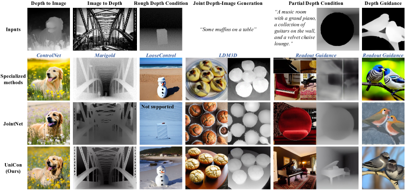
Figure 3: Qualitative comparison of diverse Image-Depth generation tasks. We compare our single UniCon-Depth model with other specialized methods and a previous unified method JointNet (Zhang et al., 2023a) on diverse generation tasks.

We base our experiments on Stable Diffusion (Rombach et al., 2022) (SD), a large-scale text-to-image diffusion model. We train 5 UniCon models, Depth, SoftEdge, Human-Pose (Pose), Human-Identity (ID), and Appearance on SDv1-5. The first three pair an image with a spatially aligned condition image. Following Luo et al. (2024), we train Depth, SoftEdge models on 16k images from PascalVOC (Everingham et al., 2012) and Pose model on a subset with 9k human images. Depth, soft edge, and pose images are estimated by Depth-Anything-v2 (Yang et al., 2024), HED (Xie & Tu, 2015) and OpenPose (Cao et al., 2019). We train the ID model on 30k human face images from CelebA (Liu et al., 2015) and use images with the same identity as training image pairs. The Appearance model, aiming at transferring one image’s appearance to another, is trained on 6k videos from Panda70M (Chen et al., 2024b). We randomly select frames in the same video clip as training image pairs. Please refer to the Appendix for other training and inference details.

5.1 Main results

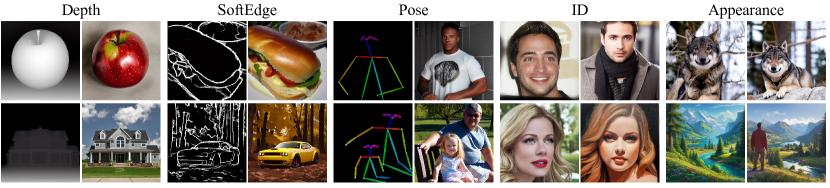
Figure 4: Conditional generation samples. We show our sample conditional generation results. For each model, the left column is the input condition and the right column is the output image.

Qualitative results. In Fig. 3, we show sample results generated by our Depth model on different tasks and compare them with a specific method for each task. Note our results are generated by the same Depth model with different sampling strategy. First, our model can accept a clean depth or image to perform Depth-to-Image or Image-to-Depth generation. ControlNet (Zhang et al., 2023b) and Marigold (Ke et al., 2024) respectively work for the two tasks with different structures. Compared to ControlNet, UniCon supports generation with a rough or partial condition. LooseControl (Bhat et al., 2024) finetunes a ControlNet for a generalized depth condition. Our model works for such created rough depth images without foreknowledge by conditioning noisy depth images. Similar to Readout-Guidance (Luo et al., 2024), we can apply the guidance on the depth output for conditional generation. In addition to a complete depth image, it is also possible to guide with part of a depth image, such as using the border of the depth map to specify the overall scene structure. Finally, our model can jointly generate an image with its depth, which is the goal of LDM3D (Stan et al., 2023).

Fig 4 shows sample results from all UniCon models. Apart from common spatial aligned control signals, our ID and Appearance models work for loosely correlated images. With the ID model, we can generate images of the same person in the condition image and utilize the input prompt to specify appearance and style. The Appearance model is trained on video frames, aiming at generating images with a similar appearance. In practice, we can set the joint cross attention weight (multiply to $\mathbf{F}^{joint}$ in Eq. 4) to allow more image variations, e.g. the same wolf with a different pose.

Table 1: Quantitative conditional generation comparison. We compare Readout-Guidance (Luo et al., 2024), ControlNet (Zhang et al., 2023b), and UniCon(Ours) on 6K validation images. For a fair comparison, all methods are trained on PascalVOC with the same annotator.

Method	Depth		SoftEdge		Pose
	FID-6K $\downarrow$	AbsRel (%) $\downarrow$	FID-6K $\downarrow$	EMSE (1e-2) $\downarrow$	FID-6K $\downarrow$	PCK @ 0.1 $\uparrow$
Readout-Guidance	18.72	23.19	18.43	4.84	21.07	24.96
ControlNet	13.68	9.85	13.46	2.30	18.61	57.54
UniCon	13.21	9.26	12.80	2.28	17.51	61.97

Table 2: Quantitative depth estimation comparison. We compare MiDaS(Ranftl et al., 2020), DPT (Ranftl et al., 2021), Marigold (Ke et al., 2024), and our Depth-Metric model on zero-shot depth estimation benchmarks. We show results without test-time ensembling.

Method	NYUv2		ScanNet
	AbsRel $\downarrow$	$\mathbf{\delta 1}$ $\uparrow$	AbsRel $\downarrow$	$\mathbf{\delta 1}$ $\uparrow$
MiDaS	11.1	88.5	12.1	84.6
DPT	9.8	90.3	8.2	93.4
Marigold	6.0	95.9	6.9	94.5
JointNet	13.7	81.9	14.7	79.5
UniCon	7.9	93.9	9.2	91.9

Quantitative comparison. We compare UniCon with other methods on conditional generation and depth estimation. For the conditional generation, we generate 6K $512\times 512$ images conditioned on depth, soft edge, or pose of random images from OpenImages (Krasin et al., 2017). We use Frechet Inception Distance (FID) (Heusel et al., 2017) to measure the distribution distance between generated images and real images corresponding to the same input conditions. We also evaluate the condition fidelity by Absolute Mean Relative Error (AbsRel) (Ke et al., 2024) for depth; Edge Mean Squared Error (EMSE) for soft edge; and Percentage of Correct Keypoints (PCK) (Yang & Ramanan, 2012) for pose. All metrics are computed between the modalities estimated from real images and generated images. For depth estimation, we evaluate on NYUv2 (Silberman et al., 2012) and ScanNet (Dai et al., 2017) with AbsRel and $\delta 1$ (Ranftl et al., 2021) as metric, following the protocol of affine invariant depth evaluation (Ranftl et al., 2020).

The conditional generation performance is related to the choice of training datasets and condition annotators. For a fair comparison, we train all models on the same dataset (PascalVOC) and annotator. We do not compare with JointNet because there is no training code provided. As shown in Tab. 1, our UniCon achieves similar or better performance than Readout-Guidance (Luo et al., 2024) and ControlNet (Zhang et al., 2023b) on FID and condition fidelity over all modalities.

We finetune our Depth model for 5K steps with Depth-Anything-V2-Metric (Yang et al., 2024) as the annotator for metric depth evaluation. As shown in Tab. 2, our Depth-Metric model performs similarly or better than MiDaS (Ranftl et al., 2020) and DPT (Ranftl et al., 2021). There is a margin between our model and Marigold (Ke et al., 2024), which fine-tunes the whole diffusion model and solely focuses on depth estimation. In comparison, our model trains fewer parameters and targets on unified conditional generation.

Flexible conditional generation. We show diverse conditional generation samples in Fig. 5. Starting from a noisy condition image, our models can interpret the exact condition image to other meanings (dog to lion in Column 1) or take rough condition as control (cat sketch in Column 2). Using guidance for partial conditioning enables us to condition on both input signals (Column 3) or repaint an image with a coarse condition signal (Column 4). We generate the ”ICLR” edge image by replacing raw edges with text.

In addition, we can combine multiple UniCon models to enhance the control ability (Fig. 8). One interesting application is to combine loose conditions (ID, Appearance) with dense conditions (Depth, Pose). In the bottom row, we use the same image for both ID and Appearance conditions to enhance both ID alignment and overall image appearance consistency. Similar to ControlNet, our models can apply to other customized checkpoints fine-tuned from our base model (Fig. 8).

Comparison with JointNet. We compare our method to the most relevant baseline, JointNet (Zhang et al., 2023a), which also supports multiple conditional generation tasks for image and depth. As demonstrated in Fig. 3, our method shows better results in image-to-depth, partial condition, and depth guidance, with extra abilities of rough depth condition. Quantitatively, UniCon achieves superior depth estimation results compared to JointNet (Tab. 2). Beyond the capabilities of JointNet, our method extends to handle non-pixel-aligned conditions (Fig. 4), supports multi-signal conditions (Fig. 8), and offers the flexibility of checkpoint switching (Fig. 8).

We also emphasize the differences in training methodology. JointNet trains on 65M images from the COYO-700M dataset (Byeon et al., 2022) on 64 NVidia A100 80G GPUs for 24 hours, including an additional fine-tuning stage for inpainting mask. It adds 889M parameters (100% of the base model SD2.1). In contrast, our UniCon-Depth trains on 16K images on 2 Nvidia A800 80G GPUs for 13 hours and adds 125M parameters (15% of the base model SDv1.5).

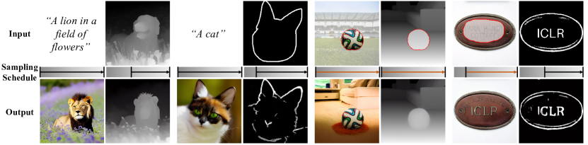
Figure 5: Flexible conditional generation via different sampling schedules. We annotate each image with its sampling schedule. Schedule bars represent the noise level from $T$ to $0$. Arrows indicate the noise sampling schedule. We apply the guidance in generation (orange arrow) for partial condition samples and use red borderlines to split areas to keep and areas to generate.

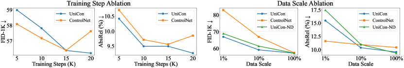
Figure 6: Ablation of training steps and data scale. We compare the depth conditional generation performance of UniCon and ControlNet on different training settings. We use the same training steps for data scale ablation and vice versa. UniCon-ND indicates trained without depth loss.

5.2 Ablation Study

Training steps and data scale. We ablate on training steps and data scale for depth conditional generation (Fig. 6). As the training step grows, our model improves steadily, showing a higher performance upper bound than ControlNet which starts to overfit on the dataset. We observe a sudden drop in condition fidelity when downscaling our training dataset. We attribute it to our joint cross-attention requiring a certain data scale to capture the image-condition correlation. On the other hand, UniCon achieves better condition fidelity with enough data.

Table 3: Ablation of training setting and model alternatives. We evaluate the conditional generation performance of our Depth model under different settings.

	FID-6K $\downarrow$	AbsRel(%) $\downarrow$
UniCon-Depth	13.21	9.26
- Depth loss	13.18	9.23
- Depth loss, noise	13.66	8.57
- Encoder	13.64	10.16
+ Data (200K)	13.10	8.66

Training setting and model alternatives. In Tab. 3, we test our Depth model with training setting and structure alternatives. First, we drop out the depth loss in training, leading to a model that has similar depth-to-image generation performance but cannot denoise depth image. We also investigate the depth loss influence under different data scales (Fig. 6 Right), showing that joint modeling depth has a positive effect on conditional generation. Further dropping the noise added to the depth image in training results in a ControlNet-like depth-control model. It improves the condition fidelity but harms generation quality. We also remove joint cross-attention modules in the UNet encoder to test the robustness against structure changes. Despite the slight performance drop, our method works with half of the attention modules. Finally, our model consistently improves when we scale up the training data to 200K images from OpenImages (Krasin et al., 2017).

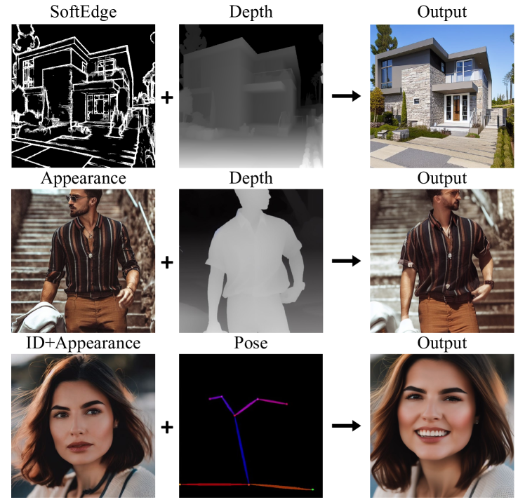
Figure 7: Multi-signal conditional generation samples. We can combine multiple models for different condition signals.

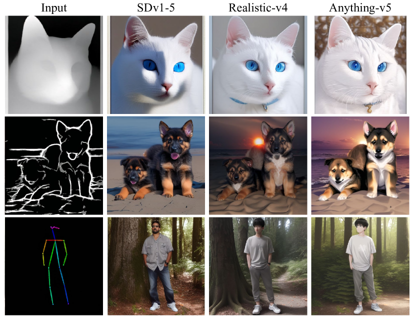
Figure 8: Apply to other checkpoints. Our models can apply to other checkpoints fine-tuned from the base model (SDv1.5).

6 Discussion

We propose a simple framework for unifying diffusion-based conditional generation. We consider all conditional generation tasks involving a specific image-condition correlation as sampling in a global distribution and train a diffusion model to learn it. Our flexible model architecture adapts a pretrained diffusion model to handle multi-input processing, alongside effective training and sampling strategies designed to support diverse generation tasks. The inherent flexibility of our approach opens up the possibility for a wide range of applications, potentially encouraging further exploration into novel image-condition mappings. Additionally, our work demonstrates that large-scale diffusion models can be successfully adapted to accommodate non-aligned noise levels in input signals, suggesting a path toward enhancing existing multi-signal diffusion models. As for limitations, some models dealing with loosely correlated image pairs, e.g. our ID model, exhibit instability. We attribute this issue to the need for more training data and refined techniques to achieve satisfactory performance in such cases.

Appendix A Implementation Details

Our model process input ${\mathbf{x}},{\mathbf{y}}$ in two parallel branches, as shown in Fig. 2. In practice, we do not prepare two network branches to process two inputs. Instead, all inputs are concatenated in batch dimension and fed into the denoising UNet, as a batch of image inputs. They are simultaneously processed, with the condition LoRA selectively applying to the ${\mathbf{y}}$ inputs. For joint cross-attention, we split ${\mathbf{x}}$ and ${\mathbf{y}}$ features and perform the cross-attention operation.

For the models we present in the paper, we use LoRA rank 64 for all adapters, including the condition LoRA and the joint cross-attention LoRA. We only add the condition LoRA when the condition image falls out of natural image distribution, i.e. our Depth, SoftEdge, and Pose models. We additionally incorporate a trigger word to the text prompts for these conditions, such as ”depth_map”.

Appendix B Training

We train 5 UniCon models, Depth, SoftEdge, Human-Pose (Pose), Human-Identity (ID), and Appearance on Stable Diffusion v1.5 (Rombach et al., 2022). Stable Diffusion uses a variational autoencoder (VAE) to define a latent space for image generation. We adopt the VAE of the base model to encode and decode all type of images to and from the latent space, including annotated images like depth, edge and pose. For all models, we use AdamW (Loshchilov, 2017) optimizer with learning rate 1e-4. The training images are resized to 512 resolution with random flipping and random cropping as data augmentation. The text prompts are generated by BLIP (Li et al., 2023; 2022) for datasets without captions. We drop out the text prompt input with a rate of 0.1 to maintain the classifier-free guidance (Ho & Salimans, 2022) ability.

Depth, SoftEdge, Pose. For spatially aligned conditions, we follow Readout-Guidance (Luo et al., 2024) to train on PascalVOC (Everingham et al., 2012). Depth and SoftEdge model is trained on 16K images and Pose model is trained on 9K images of humans. To obtain the condition input, we first annotate training images with existing estimation methods. Depth, soft edge, and pose images are estimated by Depth-Anything-v2 (Yang et al., 2024), HED (Xie & Tu, 2015) and OpenPose (Cao et al., 2019). We encode all estimated modalities as images, following the annotators in ControlNet (Zhang et al., 2023b). For SoftEdge, we follow ControlNet (Zhang et al., 2023b) to quantize the edge maps into several levels to remove possible hidden patterns. We train Depth, SoftEdge models for 20K steps with batch size 32 and Pose model for 10K steps. Training 20K steps costs about 13 hours on two NVIDIA A800 80G GPUs. To adapt our Depth model for metric depth estimation, we further fine-tune the model for 5K steps on images annotated with Depth-Anything-v2-Metric. The produced Depth-Metric model is used for the depth estimation evaluation in Tab. 2.

ID, Appearance. We test our method on two cases of loosely correlated image pairs, the identity-preserving model and the appearance-preserving model. The Identity model is trained on human images with the same identity. We collect 30K human images from CelebA (Liu et al., 2015), including about 5K identities with more than 1 image. We randomly pair images with the same ID to generate 200K training image pairs (50 for each identity). We train the Appearance model on Panda-70M (Chen et al., 2024b). Due to issues in downloading YouTube videos in Panda-70M, we only use a minimal subset with 6K videos for training. When training, we load video clips with a length of 16 and a resampled frame rate of 7 and randomly select two frames from loaded clips as input image pairs. The ID and Appearance models are trained for 20k steps with batch size 64 distributed on 4 NVIDIA A800 80G GPUs.

Appendix C Inference

Table 4: Example sampling schedules for different conditional generation targets given a UniCon model of ${\mathbf{x}},{\mathbf{y}}$.

Target	Example Sampling Schedule (50 steps)
$p({\mathbf{x}},{\mathbf{y}})$	$({\mathbf{x}}_{50},{\mathbf{y}}_{50}),({\mathbf{x}}_{49},{\mathbf{y}}_{49}),...,({\mathbf{x}}_{1},{\mathbf{y}}_{1}),({\mathbf{x}}_{0},{\mathbf{y}}_{0})$
$p({\mathbf{y}}|{\mathbf{x}}_{0})$	$({\mathbf{x}}_{0},{\mathbf{y}}_{50}),({\mathbf{x}}_{0},{\mathbf{y}}_{49}),...,({\mathbf{x}}_{0},{\mathbf{y}}_{1}),({\mathbf{x}}_{0},{\mathbf{y}}_{0})$
$p({\mathbf{x}}|{\mathbf{y}}_{0})$	$({\mathbf{x}}_{50},{\mathbf{y}}_{0}),({\mathbf{x}}_{49},{\mathbf{y}}_{0}),...,({\mathbf{x}}_{1},{\mathbf{y}}_{0}),({\mathbf{x}}_{0},{\mathbf{y}}_{0})$
$p({\mathbf{x}}|{\mathbf{y}}_{25})$	$({\mathbf{x}}_{50},{\mathbf{y}}_{25}),({\mathbf{x}}_{49},{\mathbf{y}}_{25}),({\mathbf{x}}_{48},{\mathbf{y}}_{24}),...,({\mathbf{x}}_{1},{\mathbf{y}}_{1}),({\mathbf{x}}_{0},{\mathbf{y}}_{0})$
$p({\mathbf{x}}|{\mathbf{y}}^{m}_{0})$	$({\mathbf{x}}_{50},{\mathbf{y}}_{50}),({\mathbf{x}}^{g(y^{m}_{0})}_{49},{\mathbf{y}}^{g(y^{m}_{0})}_{49}),...,({\mathbf{x}}^{g(y^{m}_{0})}_{1},{\mathbf{y}}^{g(y^{m}_{0})}_{1}),({\mathbf{x}}^{g(y^{m}_{0})}_{0},{\mathbf{y}}^{g(y^{m}_{0})}_{0})$

Sampling schedules. In Tab 4, we list example sampling schedules to show how our sampling strategies (discussed in Sec. 4.3) support the conditional sampling described in Eq. 3. For the partial conditioning case $p({\mathbf{x}}|{\mathbf{y}}^{m}_{0})$, $g({\mathbf{y}}^{m}_{0})$ means replacing latents and applying guidance according to give masked condition ${\mathbf{y}}^{m}_{0}$ (Sec. 4.3, Sampling with guidance). Note that the listed sampling schedule is one possible schedule to achieve the target. We can alter or combine them to perform customized conditional generation. For guidance, we adopt an optimizer (e.g. AdamW) to compute the gradient and determine the weighting factor $w_{r}$ in Eq. 7 instead of manually setting a fixed weight factor, as suggested by Readout-Guidance (Luo et al., 2024).

Combining multiple models. As discussed in Sec. 4.3, we can combine multiple UniCon models to achieve multi-signal control. We expand the details here. Suppose we have input image ${\mathbf{x}}$ and two input conditions ${\mathbf{y}},{\mathbf{z}}$. We denote the model parameters for ${\mathbf{y}}$ and ${\mathbf{z}}$ as $\theta_{y},\theta_{z}$. Then the joint feature outputs $\mathbf{F}^{joint}_{x},\mathbf{F}^{joint}_{y},\mathbf{F}^{joint}_{z}$ in Eq. 4 are computed as:

$$\begin{split}&\mathbf{F}_{xy},\mathbf{F}_{yx}=\text{JointCrossAttn}(\mathbf{F}_{x}^{\textrm{in}},\mathbf{F}_{y}^{\textrm{in}};\theta_{y}),\mathbf{F}_{xz},\mathbf{F}_{zx}=\text{JointCrossAttn}(\mathbf{F}_{x}^{\textrm{in}},\mathbf{F}_{z}^{\textrm{in}};\theta_{z}),\\ &\mathbf{F}^{joint}_{x}=w_{xy}\mathbf{F}_{xy}+w_{xz}\mathbf{F}_{xz},\mathbf{F}^{joint}_{y}=w_{yx}\mathbf{F}_{yx},\mathbf{F}^{joint}_{z}=w_{zx}\mathbf{F}_{zx},\end{split}$$ (8)

where all $w$ are weighting factors to balance the strength of each condition. To explain, we perform joint cross-attention between any image-condition pairs $({\mathbf{x}},{\mathbf{y}})$ and $({\mathbf{x}},{\mathbf{z}})$ with corresponding model weights. Then the image branch will aggregate all output features as the final output.

Condition Guidance. Our ID and Appearance models that target a loose correlation sometimes perform badly in the conditional generation, generating low-quality images or images not aligned with the condition. We attribute the problem to the fact that loose condition has a weaker influence on image generation as it allows more freedom and diversity in generated images than dense conditions. Similar problems have also been observed in text-to-image generation, with an effective solution called classifier-free guidance (Ho & Salimans, 2021). Therefore, we optionally utilize a similar guidance scheme to emphasize a certain condition signal for better condition alignment.

In specific, we alter the model output as $\bm{\epsilon}_{g}=\bm{\epsilon}_{sep}+k(\bm{\epsilon}_{joint}-\bm{\epsilon}_{sep})$ where $\bm{\epsilon}_{joint},\bm{\epsilon}_{sep}$ are the model output with or without joint cross-attention and $k$ is the guidance scale. Intuitively, the output towards the direction defined by $\bm{\epsilon}_{joint}-\bm{\epsilon}_{sep}$, which means the condition signal from joint cross-attention is enhanced. Furthermore, we can enable more fine-grained guidance over a specific signal when there are multiple condition signals by replacing $\bm{\epsilon}_{joint},\bm{\epsilon}_{sep}$ with $\bm{\epsilon}({\bm{w}}_{con}),\bm{\epsilon}({\bm{w}}_{unc})$. Here ${\bm{w}}_{con},{\bm{w}}_{unc}$ indicate the two sets of weighting factors used in Eq. 8. Therefore $\bm{\epsilon}({\bm{w}}_{con}),\bm{\epsilon}({\bm{w}}_{unc})$ are the model output with different condition weighing factors. Take Eq 8 as an example, if we want to emphasize ${\mathbf{y}}$ but not ${\mathbf{z}}$, we can set $w_{xy},w_{yx}$ to 1 in ${\bm{w}}_{con}$ and to 0 in ${\bm{w}}_{unc}$ while keeping other weights the same.

Appendix D Evaluation

D.1 Evaluation Metrics

For conditional generation (Tab. 1), we compute Frechet Inception Distance (FID) (Heusel et al., 2017) between 6K generated images and corresponding real images. We measure condition fidelity using an estimation-matching strategy. In specific, we estimate the condition modalities of the generated images and real images. Then, we compute alignment metrics over the attributes estimated on the generated images and on the real images, to measure the alignment between reference and generated images on the condition modality.

Depth alignment. We compute the Absolute Mean Relative Error (Ke et al., 2024) (AbsRel) on depth values estimated by Depth-Anything-V2. We adopt the same affine-invariant evaluation protocol as our depth estimation evaluation.

Edge alignment. For edge alignment, we simply compute the mean squared error on non-zero areas (i.e. edge areas) in the estimated edge maps, thus denoting it as Edge Mean Squared Error (EMSE). Because the edge map is nearly a binary value map, EMSE can directly reflect the alignment of edges.

Pose alignment. For pose alignment, we compute the standard pose estimation metric Percentage of Correct Keypoints (Yang & Ramanan, 2012) (PCK) with an adaptation to fit our scenario. PCK measures the alignment between paired ground truth and predicted keypoints. However, the real and generated images in our evaluation may include multiple humans, and we do not have a matching between them. Therefore, we perform a greedy matching between real image keypoints and generated image keypoints. In specific, we compute pair-wise PCK across all sets of keypoints in two images. Then we match the keypoints set greedily in PCK descending order and obtain a matching between two groups of keypoints. Finally, we compute PCK over the matched keypoints.

For depth estimation evaluation, we follow the same affine-invariant evaluation setting as Marigold (Ke et al., 2024), i.e. aligning the prediction with ground truth with the least squares fitting. Suppose ${\mathbf{a}}$ is the predicted depth and ${\mathbf{d}}$ is the GT depth. We compute AbsRel as $\frac{1}{M}\sigma_{i=1}^{M}|{\mathbf{a}}_{i}-{\mathbf{d}}_{i}|/{\mathbf{d}}_{i}$ where $M$ is the total number of pixels. Another metric $\delta_{1}$ is defined as the proportion of pixels satisfying $\max({\mathbf{a}}_{i}/{\mathbf{d}}_{i},{\mathbf{d}}_{i}/{\mathbf{a}}_{i})<1.25$.

D.2 Sampling Setting

For conditional generation comparison in Tab. 1, we use the DDIM (Song et al., 2020a) scheduler with eta=1.0. We sample for 50 steps and use a classifier-free guidance scale of 7.5. We use identical sampling settings for all comparison methods. For depth estimation in Tab. 2, we use the Euler Ancestral scheduler (Karras et al., 2022) to sample 20 steps. Additionally, we find adding a minor noise (10% of max noise timestep) to the input image helps improve the estimation quality.

For the qualitative comparison in Fig. 3, we generate specialized methods with their default sampling setting. JointNet (Zhang et al., 2023a) does not support guidance in their official implementation. Therefore, we adopt the same guidance scheme on their model to generate the depth guidance sample. We tune our sampling setting to generate each sample, such as the noise level added to the input depth for the rough depth condition task.

Appendix E Additional Results

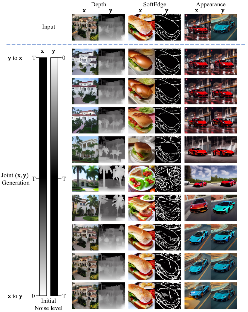
Figure 9: Interpolating noise schedules. We can move from ${\mathbf{x}}$-to-${\mathbf{y}}$ generation to ${\mathbf{y}}$-to-${\mathbf{x}}$ generation by interpolating the level of initial noise added to ${\mathbf{x}},{\mathbf{y}}$ inputs. After adding the noise, we denoise ${\mathbf{x}},{\mathbf{y}}$ together to clean outputs.

In Fig. 9, we show that we can interpolate the initial noise levels for input ${\mathbf{x}},{\mathbf{y}}$ to gradually change our sampling behavior in ${\mathbf{y}}$-to-${\mathbf{x}}$, rough ${\mathbf{y}}$-to-${\mathbf{x}}$, joint ${\mathbf{x}},{\mathbf{y}}$ generation, rough ${\mathbf{x}}$-to-${\mathbf{y}}$, and ${\mathbf{x}}$-to-${\mathbf{y}}$.

References

- Baldridge et al. (2024) Jason Baldridge, Jakob Bauer, Mukul Bhutani, Nicole Brichtova, Andrew Bunner, Kelvin Chan, Yichang Chen, Sander Dieleman, Yuqing Du, Zach Eaton-Rosen, et al. Imagen 3. arXiv preprint arXiv:2408.07009, 2024.
- Bhat et al. (2024) Shariq Farooq Bhat, Niloy Mitra, and Peter Wonka. Loosecontrol: Lifting controlnet for generalized depth conditioning. In SIGGRAPH, 2024.
- Byeon et al. (2022) Minwoo Byeon, Beomhee Park, Haecheon Kim, Sungjun Lee, Woonhyuk Baek, and Saehoon Kim. Coyo-700m: Image-text pair dataset. https://github.com/kakaobrain/coyo-dataset, 2022.
- Cao et al. (2019) Z. Cao, G. Hidalgo Martinez, T. Simon, S. Wei, and Y. A. Sheikh. Openpose: Realtime multi-person 2d pose estimation using part affinity fields. IEEE TPAMI, 2019.
- Chen et al. (2024a) Boyuan Chen, Diego Marti Monso, Yilun Du, Max Simchowitz, Russ Tedrake, and Vincent Sitzmann. Diffusion forcing: Next-token prediction meets full-sequence diffusion. arXiv preprint arXiv:2407.01392, 2024a.
- Chen et al. (2024b) Tsai-Shien Chen, Aliaksandr Siarohin, Willi Menapace, Ekaterina Deyneka, Hsiang-wei Chao, Byung Eun Jeon, Yuwei Fang, Hsin-Ying Lee, Jian Ren, Ming-Hsuan Yang, et al. Panda-70m: Captioning 70m videos with multiple cross-modality teachers. In CVPR, 2024b.
- Couairon et al. (2023) Guillaume Couairon, Mohamed Elgharib, Kiran Varanasi, Alexis Joly, Patrick Pérez, and Cordelia Schmid. Diffedit: Diffusion-based semantic image editing with mask guidance. arXiv preprint arXiv:2303.09367, 2023.
- Dai et al. (2017) Angela Dai, Angel X Chang, Manolis Savva, Maciej Halber, Thomas Funkhouser, and Matthias Nießner. Scannet: Richly-annotated 3d reconstructions of indoor scenes. In CVPR, 2017.
- Everingham et al. (2012) M. Everingham, L. Van Gool, C. K. I. Williams, J. Winn, and A. Zisserman. The PASCAL Visual Object Classes Challenge 2012 (VOC2012) Results. http://www.pascal-network.org/challenges/VOC/voc2012/workshop/index.html, 2012.
- Guo et al. (2024) Yuwei Guo, Ceyuan Yang, Anyi Rao, Zhengyang Liang, Yaohui Wang, Yu Qiao, Maneesh Agrawala, Dahua Lin, and Bo Dai. Animatediff: Animate your personalized text-to-image diffusion models without specific tuning. ICLR, 2024.
- Heusel et al. (2017) Martin Heusel, Hubert Ramsauer, Thomas Unterthiner, Bernhard Nessler, and Sepp Hochreiter. Gans trained by a two time-scale update rule converge to a local nash equilibrium. Adv. Neural Inform. Process. Syst., 30, 2017.
- Ho & Salimans (2021) Jonathan Ho and Tim Salimans. Classifier-free diffusion guidance. In NeurIPS 2021 Workshop on Deep Generative Models and Downstream Applications, 2021.
- Ho & Salimans (2022) Jonathan Ho and Tim Salimans. Classifier-free diffusion guidance. arXiv preprint arXiv:2207.12598, 2022.
- Ho et al. (2020) Jonathan Ho, Ajay Jain, and Pieter Abbeel. Denoising diffusion probabilistic models. NeurIPS, 2020.
- Ho et al. (2022a) Jonathan Ho, William Chan, Chitwan Saharia, Jay Whang, Ruiqi Gao, Alexey Gritsenko, Diederik P Kingma, Ben Poole, Mohammad Norouzi, David J Fleet, et al. Imagen video: High definition video generation with diffusion models. arXiv preprint arXiv:2210.02303, 2022a.
- Ho et al. (2022b) Jonathan Ho, Tim Salimans, Alexey Gritsenko, William Chan, Mohammad Norouzi, and David J. Fleet. Video diffusion models. arXiv preprint arXiv:2204.03458, 2022b.
- Hu et al. (2021) Edward J Hu, Phillip Wallis, Zeyuan Allen-Zhu, Yuanzhi Li, Shean Wang, Lu Wang, Weizhu Chen, et al. Lora: Low-rank adaptation of large language models. In ICLR, 2021.
- Huang et al. (2023) Lianghua Huang, Di Chen, Yu Liu, Yujun Shen, Deli Zhao, and Jingren Zhou. Composer: Creative and controllable image synthesis with composable conditions. arXiv preprint arXiv:2302.09778, 2023.
- Karras et al. (2022) Tero Karras, Miika Aittala, Timo Aila, and Samuli Laine. Elucidating the design space of diffusion-based generative models. NeurIPS, 2022.
- Ke et al. (2024) Bingxin Ke, Anton Obukhov, Shengyu Huang, Nando Metzger, Rodrigo Caye Daudt, and Konrad Schindler. Repurposing diffusion-based image generators for monocular depth estimation. In CVPR, 2024.
- Krasin et al. (2017) Ivan Krasin, Tom Duerig, Neil Alldrin, Vittorio Ferrari, Sami Abu-El-Haija, Alina Kuznetsova, Hassan Rom, Jasper Uijlings, Stefan Popov, Andreas Veit, Serge Belongie, Victor Gomes, Abhinav Gupta, Chen Sun, Gal Chechik, David Cai, Zheyun Feng, Dhyanesh Narayanan, and Kevin Murphy. Openimages: A public dataset for large-scale multi-label and multi-class image classification. Dataset available from https://github.com/openimages, 2017.
- Li et al. (2022) Junnan Li, Dongxu Li, Caiming Xiong, and Steven Hoi. Blip: Bootstrapping language-image pre-training for unified vision-language understanding and generation. In ICML, 2022.
- Li et al. (2023) Junnan Li, Dongxu Li, Silvio Savarese, and Steven Hoi. Blip-2: Bootstrapping language-image pre-training with frozen image encoders and large language models. In ICML, 2023.
- Liu et al. (2023) Xian Liu, Jian Ren, Aliaksandr Siarohin, Ivan Skorokhodov, Yanyu Li, Dahua Lin, Xihui Liu, Ziwei Liu, and Sergey Tulyakov. Hyperhuman: Hyper-realistic human generation with latent structural diffusion. arXiv preprint arXiv:2310.08579, 2023.
- Liu et al. (2015) Ziwei Liu, Ping Luo, Xiaogang Wang, and Xiaoou Tang. Deep learning face attributes in the wild. In ICCV, 2015.
- Loshchilov (2017) I Loshchilov. Decoupled weight decay regularization. arXiv preprint arXiv:1711.05101, 2017.
- Luo et al. (2024) Grace Luo, Trevor Darrell, Oliver Wang, Dan B Goldman, and Aleksander Holynski. Readout guidance: Learning control from diffusion features. In CVPR, 2024.
- Meng et al. (2021) Chenlin Meng, Yutong He, Yang Song, Jiaming Song, Jiajun Wu, Jun-Yan Zhu, and Stefano Ermon. Sdedit: Guided image synthesis and editing with stochastic differential equations. In ICLR, 2021.
- Midjourney (2023) Midjourney. https://www.midjourney.com/, 2023.
- Mou et al. (2023) Chong Mou, Xintao Wang, Liangbin Xie, Jian Zhang, Zhongang Qi, Ying Shan, and Xiaohu Qie. T2i-adapter: Learning adapters to dig out more controllable ability for text-to-image diffusion models. arXiv preprint arXiv:2302.08453, 2023.
- Nam et al. (2024) Jisu Nam, Gyuseong Lee, Sunwoo Kim, Hyeonsu Kim, Hyoungwon Cho, Seyeon Kim, and Seungryong Kim. Diffusion model for dense matching. In ICLR, 2024.
- OpenAI (2023) OpenAI. Dall-e-2, https://openai.com/product/dall-e-2, 2023.
- Qi et al. (2024) Lu Qi, Lehan Yang, Weidong Guo, Yu Xu, Bo Du, Varun Jampani, and Ming-Hsuan Yang. Unigs: Unified representation for image generation and segmentation. In CVPR, 2024.
- Ramesh et al. (2022) Aditya Ramesh, Prafulla Dhariwal, Alex Nichol, Casey Chu, and Mark Chen. Hierarchical text-conditional image generation with clip latents. arXiv preprint arXiv:2204.06125, 2022.
- Ranftl et al. (2020) René Ranftl, Katrin Lasinger, David Hafner, Konrad Schindler, and Vladlen Koltun. Towards robust monocular depth estimation: Mixing datasets for zero-shot cross-dataset transfer. IEEE TPAMI, 44(3):1623–1637, 2020.
- Ranftl et al. (2021) René Ranftl, Alexey Bochkovskiy, and Vladlen Koltun. Vision transformers for dense prediction. In ICCV, 2021.
- Rombach et al. (2022) Robin Rombach, Andreas Blattmann, Dominik Lorenz, Patrick Esser, and Björn Ommer. High-resolution image synthesis with latent diffusion models. In CVPR, 2022.
- Ronneberger et al. (2015) Olaf Ronneberger, Philipp Fischer, and Thomas Brox. U-net: Convolutional networks for biomedical image segmentation. In Medical Image Computing and Computer-Assisted Intervention, 2015.
- Saxena et al. (2023a) Saurabh Saxena, Charles Herrmann, Junhwa Hur, Abhishek Kar, Mohammad Norouzi, Deqing Sun, and David J. Fleet. The surprising effectiveness of diffusion models for optical flow and monocular depth estimation. In NeurIPS, 2023a.
- Saxena et al. (2023b) Saurabh Saxena, Junhwa Hur, Charles Herrmann, Deqing Sun, and David J Fleet. Zero-shot metric depth with a field-of-view conditioned diffusion model. arXiv preprint arXiv:2312.13252, 2023b.
- Silberman et al. (2012) Nathan Silberman, Derek Hoiem, Pushmeet Kohli, and Rob Fergus. Indoor segmentation and support inference from rgbd images. In ECCV, 2012.
- Sohl-Dickstein et al. (2015) Jascha Sohl-Dickstein, Eric Weiss, Niru Maheswaranathan, and Surya Ganguli. Deep unsupervised learning using nonequilibrium thermodynamics. In ICML, 2015.
- Sohn et al. (2023) Kihyuk Sohn, Nataniel Ruiz, Kimin Lee, Daniel Castro Chin, Irina Blok, Huiwen Chang, Jarred Barber, Lu Jiang, Glenn Entis, Yuanzhen Li, et al. Styledrop: Text-to-image generation in any style. arXiv preprint arXiv:2306.00983, 2023.
- Song et al. (2020a) Jiaming Song, Chenlin Meng, and Stefano Ermon. Denoising diffusion implicit models. In ICLR, 2020a.
- Song et al. (2020b) Yang Song, Jascha Sohl-Dickstein, Diederik P Kingma, Abhishek Kumar, Stefano Ermon, and Ben Poole. Score-based generative modeling through stochastic differential equations. In ICML, 2020b.
- Stan et al. (2023) Gabriela Ben Melech Stan, Diana Wofk, Scottie Fox, Alex Redden, Will Saxton, Jean Yu, Estelle Aflalo, Shao-Yen Tseng, Fabio Nonato, Matthias Muller, et al. Ldm3d: Latent diffusion model for 3d. arXiv preprint arXiv:2305.10853, 2023.
- Tumanyan et al. (2023) Narek Tumanyan, Michal Geyer, Shai Bagon, and Tali Dekel. Plug-and-play diffusion features for text-driven image-to-image translation. In CVPR, 2023.
- Xie & Tu (2015) Saining Xie and Zhuowen Tu. Holistically-nested edge detection. In ICCV, 2015.
- Xu et al. (2023) Jiarui Xu, Sifei Liu, Arash Vahdat, Wonmin Byeon, Xiaolong Wang, and Shalini De Mello. Open-vocabulary panoptic segmentation with text-to-image diffusion models. In CVPR, 2023.
- Yang et al. (2024) Lihe Yang, Bingyi Kang, Zilong Huang, Zhen Zhao, Xiaogang Xu, Jiashi Feng, and Hengshuang Zhao. Depth anything v2. arXiv preprint arXiv:2406.09414, 2024.
- Yang & Ramanan (2012) Yi Yang and Deva Ramanan. Articulated human detection with flexible mixtures of parts. IEEE TPAMI, 35(12):2878–2890, 2012.
- Ye et al. (2023) Hu Ye, Jun Zhang, Sibo Liu, Xiao Han, and Wei Yang. Ip-adapter: Text compatible image prompt adapter for text-to-image diffusion models. arXiv preprint arXiv:2308.06721, 2023.
- Zeng et al. (2024) Yu Zeng, Vishal M Patel, Haochen Wang, Xun Huang, Ting-Chun Wang, Ming-Yu Liu, and Yogesh Balaji. Jedi: Joint-image diffusion models for finetuning-free personalized text-to-image generation. In CVPR, 2024.
- Zhang et al. (2023a) Jingyang Zhang, Shiwei Li, Yuanxun Lu, Tian Fang, David McKinnon, Yanghai Tsin, Long Quan, and Yao Yao. Jointnet: Extending text-to-image diffusion for dense distribution modeling. arXiv preprint arXiv:2310.06347, 2023a.
- Zhang et al. (2023b) Lvmin Zhang, Anyi Rao, and Maneesh Agrawala. Adding conditional control to text-to-image diffusion models. In ICCV, 2023b.
- Zhao et al. (2023) Wenliang Zhao, Yongming Rao, Zuyan Liu, Benlin Liu, Jie Zhou, and Jiwen Lu. Unleashing text-to-image diffusion models for visual perception. In ICCV, 2023.