The nature of low-luminosity AGNs discovered by JWST at $5<z<6$ based on clustering analysis: ancestors of quasars at $z\lesssim 3$?

Abstract

James Webb Space Telescope (JWST) has discovered many faint AGNs at high-$z$ by detecting their broad Balmer lines. However, their high number density, lack of X-ray emission, and overly high black hole masses with respect to their host stellar masses suggest that they are a distinct population from general type-1 quasars. Here, we present clustering analysis of 28 low-luminosity broad-line AGNs found by JWST (JWST AGNs) at $5<z<6$ based on cross-correlation analysis with 679 photometrically-selected galaxies to characterize their host dark matter halo (DMH) masses. From angular and projected cross-correlation functions, we find that their typical DMH mass is $\log(M_{\mathrm{halo}}/h^{-1}\mathrm{M_{\odot}})=11.61_{-0.24}^{+0.19},$ and $11.72_{-0.20}^{+0.17}$, respectively. This result implies that the host DMHs of these AGNs are $\sim 1$ dex smaller than that of luminous quasars. The DMHs of JWST AGNs at $5<z<6$ are predicted to grow to $10^{12\,\mathchar 45\relax 13}\,h^{-1}\mathrm{M_{\odot}}$, a typical mass of quasar at $z\lesssim 3$. Applying the empirical stellar-to-halo mass ratio to the measured DMH mass, their host stellar mass is evaluated as $\log(M_{*}/\mathrm{M_{\odot}})=9.72_{-0.39}^{+0.31},$ and $9.90_{-0.33}^{+0.27}$, which are higher than some of those estimated by the SED fitting. We also evaluate their duty cycle as $f_{\mathrm{duty}}=0.36_{-0.14}^{+0.18}$ per cent, namely $\sim 7\times 10^{6}$ yr as the lifetime of JWST AGNs. While we cannot exclude the possibility that JWST AGNs are simply low-mass type-1 quasars, these results suggest that JWST AGNs are a different population from type-1 quasars, and may be the ancestors of quasars at $z\lesssim 3$.

1 Introduction

Active Galactic Nuclei (AGNs) are the extremely bright population in the Universe. Driven by the central supermassive black holes (SMBHs) (Kormendy & Richstone, 1995), the AGNs outshine their host galaxies by releasing the part of the gravitational potential of accreting massive gas and stars onto the accretion disks as radiant energy (Salpeter, 1964; Lynden-Bell, 1969). Many previous measurements suggest a relationship between the SMBH mass and the host stellar mass (Kormendy & Ho, 2013), implying co-evolution between SMBHs and host galaxies. Unveiling the mechanism of co-evolution is one of the greatest goals of the modern galactic astronomy.

Recently, deep IR observation by the James Webb Space Telescope (JWST) discovered many low-luminosity objects with broad Balmer lines with $\mathrm{FWHM}\gtrsim 1000\,\mathrm{km\,s^{-1}}$ at $4<z<7$ (e.g. Kocevski et al., 2023; Maiolino et al., 2023; Harikane et al., 2023; Greene et al., 2024; Matthee et al., 2024; Kocevski et al., 2024). The origin of the broad lines for the objects is under debate, but they are usually believed to originate in the broad line regions in AGNs; therefore we hereafter call these objects JWST AGNs. The high sensitivity of the JWST observation allows the study of AGNs that are much fainter ($M_{UV}\sim-17$) and have been unexplored by ground-based telescope observations. In addition, JWST discovers remarkable objects named little red dots (LRDs), one of the populations in the JWST AGNs, which are characterised by blue UV excess and red optical slope and compactness (Kokorev et al., 2023; Barro et al., 2024; Greene et al., 2024; Kocevski et al., 2024; Wang et al., 2024; Akins et al., 2024). JWST has played an important role in recent AGN science, especially at high-$z$, and is accelerating its progress.

The observed number density of JWST AGNs is $>2\mathchar 45\relax 3$ dex higher than the extrapolation to the faint-end of the quasar luminosity functions (Maiolino et al., 2023; Harikane et al., 2023; Kocevski et al., 2024). If their escape fraction of ionizing photon is as high as that of quasars, JWST AGNs may play a non-negligible role in the reionization (e.g. Giallongo et al., 2015; Finkelstein et al., 2019; Giallongo et al., 2019; Boutsia et al., 2021; Grazian et al., 2022). In that case, a modification would be required to the current prevailing reionization scenario, in which star-forming galaxies are the main contributors (Robertson et al., 2015). In addition, JWST AGNs display some unfamiliar features. Padmanabhan & Loeb (2023) argued that the X-ray background would be inconsistent with the current observation if overabundant JWST AGNs emit X-rays as strong as quasars, which implies that JWST AGNs may be different from normal quasars. Yue et al. (2024) obtained tentative detections from the stacked X-ray images of 34 spectroscopically confirmed LRDs in both soft (0.5-2 keV) and hard bands (2-8 keV) with $2.9\sigma$ and $3.2\sigma$ significance, respectively, although the empirical relation with H$\alpha$ luminosity suggests clear detection of X-ray emission. Maiolino et al. (2024) also reported that the majority of the 71 JWST AGNs at $2<z<11$ were not detected by the Chandra observation. Maiolino et al. (2023) found that most of the JWST AGNs have significantly overmassive SMBHs compared with their host stellar mass. The deviation from the local relation (e.g. Reines & Volonteri, 2015) is difficult to explain only by the selection effect. Pérez-González et al. (2024) suggested from MIRI observations that many of the observed LRDs may be extremely intense and compact starburst galaxies based on the best-fitting spectral energy distribution (SED) models. Kokubo & Harikane (2024) reported, based on multi-epoch photometry of five broad H$\alpha$ emitters and LRDs, no time variability of AGNs with $M_{\mathrm{BH}}\sim 10^{7}\,\mathrm{M_{\odot}}$, even though their typical timescales are shorter than the sampling interval. They also suggest that the origin of the broad lines other than AGNs may be unusually fast outflows or Raman scattering of stellar UV continua. This situation strongly recommends that we should elucidate the nature of JWST AGNs.

While multiwavelength observations are effective methods to explore the nature of JWST AGNs, clustering analysis is also useful in differentiating them from quasars. Clustering analysis can reveal the typical dark matter halo (DMH) mass of the objects. The gravitational potential of DMHs plays an important role in accumulating the gas, which is consumed to form stars; hence more massive DMHs can harbour galaxies with more massive stellar mass (White & Rees, 1978). Referring to the DMH mass function for the DMH mass range of quasars derived by clustering analysis deduces the number density of entire SMBHs in the Universe. Comparing the number density with that of quasars estimated by the luminosity function derives the fraction of active SMBHs, which can be regarded as a duty cycle. These physical quantities, especially in the early Universe, are key to understanding how the co-evolution is constructed and how SMBHs with $M_{\mathrm{BH}}\gtrsim 10^{8}\,\mathrm{M_{\odot}}$ are formed (e.g. Mortlock et al., 2011; Bañados et al., 2018; Matsuoka et al., 2019; Yang et al., 2020; Koptelova & Hwang, 2022).

Recently, it has become possible to evaluate the auto-correlation function of quasars even at $z\sim 6$ owing to the high sensitivity and the large FoV of Hyper Suprime-Cam on the Subaru Telescope. Arita et al. (2023) used 107 quasars identified spectroscopically in Subaru High-$z$ Exploration of Low-Luminosity Quasars (SHELLQs; Matsuoka et al., 2016) and reported that the typical DMH mass of quasars at $z\sim 6$ is $\log(M_{\mathrm{halo}}/h^{-1}\mathrm{M_{\odot}})=12.7_{-0.7}^{+0.4}$. They found that the typical DMH mass of type-1 quasars does not change over cosmic time. They also deduce the host stellar mass of quasars as $\log(M_{*}/\mathrm{M_{\odot}})=10.97_{-0.70}^{+0.39}$ assuming the empirical relation between the DMH mass and the stellar mass (Behroozi et al., 2019). Eilers et al. (2024) performed cross-correlation analysis with four bright quasars and surrounding [O iii] emitters by JWST NIRCam’s slitless spectroscopy (Emission-line galaxies and Intergalactic Gas in the Epoch of Reionization, EIGER; Kashino et al., 2023) and estimated the minimum DMH mass to host a quasar as $\log(M_{\mathrm{halo},\mathrm{min}})=12.30\pm 0.14$. They also estimated the duty cycle as $f_{\mathrm{duty}}=0.08_{-0.06}^{+0.17}\%$.

In this paper, we perform the clustering analysis of JWST AGNs to unveil their DMH mass. Although many AGN candidates have already been reported in the JWST public data (e.g.Kokorev et al., 2024b; Kocevski et al., 2024; Akins et al., 2024) and the number of spectroscopically confirmed AGNs is increasing (e.g.Maiolino et al., 2023; Harikane et al., 2023; Greene et al., 2024; Matthee et al., 2024; Kocevski et al., 2024), the survey area is still small and their surface number density is not yet sufficient to evaluate their auto-correlation signal. Therefore, in order to obtain more robust signals, we perform cross-correlation analysis with JWST AGNs and surrounding galaxies. Based on the comparison of the DMH mass between JWST AGNs and quasars, we discuss whether JWST AGNs and quasars are the same populations. In addition, we also calculate the host stellar mass and duty cycle of JWST AGNs and track $M_{\mathrm{BH}}/M_{*}$, which can provide additional information on the nature of JWST AGNs.

The structure of this paper is as follows. We remark on the JWST AGN and galaxy sample and their selection to evaluate the correlation functions in Section 2. Section 3 presents the details of the clustering analysis based on the angular correlation function (Section 3.1) and the projected correlation function (Section 3.2). In Section 4, we show our results and compare them with previous studies executing the clustering analysis with quasars. We summarise our results and conclude in Section 5. We adopt flat $\Lambda$ cold dark matter cosmology with $h=0.7$, $\Omega_{m}=0.3$, $\Omega_{\lambda}=0.7$, and $\sigma_{8}=0.81$ through this paper. All magnitudes in this paper are presented in the AB system (Oke & Gunn, 1983).

2 Data and Sample Selection

2.1 JWST AGNs

We select JWST AGNs by compiling the literature on spectroscopic observation of AGNs with NIRSpec or NIRCam grism (Maiolino et al., 2023; Harikane et al., 2023; Kocevski et al., 2024; Matthee et al., 2024) identified in the following public fields: the JWST Advanced Deep Extragalactic Survey (JADES; Eisenstein et al., 2023); First Reionization Epoch Spectroscopically Complete Observations (FRESCO; Oesch et al., 2023); Cosmic Evolution Early Release Science Survey (CEERS; Finkelstein et al., 2023); Public Release IMaging for Extragalactic Research (PRIMER) survey (Dunlop et al., 2021). We note that some of the JWST AGNs in the CEERS field are excluded because they are located in the region where only NIRSpec observation is performed, hence there are no catalogued galaxies with NIRCam photometry around them. We only use spectroscopically confirmed AGNs with broad Balmer line components with $\mathrm{FWHM}\gtrsim 1000\,\mathrm{km\,s^{-1}}$, i.e., the same feature as type-1 AGNs. AGNs with only narrow Balmer lines that do not meet the above conditions are excluded here, because the clustering strength of obscured AGNs may differ from that of type-1 AGNs (e.g. Hickox et al., 2011). No limits are placed on the luminosity of JWST AGNs, assuming that the clustering strength of the JWST AGN, like the type-1 AGN, is independent of luminosity (Croom et al., 2005; Adelberger et al., 2006; Myers et al., 2006; Shen et al., 2009), and we emphasise that this analysis does not need the intrinsic bolometric luminosity, which may be underestimated due to heavy obscuration (e.g. Kocevski et al., 2024) of JWST AGNs. Although no limits are set for luminosity, in the end, the AGNs selected by JWST are limited to those with lower luminosity ($-17<M_{UV}<-20$) than quasars. Figure 1 shows the redshift distribution of JWST AGNs in the literature, showing that the number is the highest at $5<z<6$. Hence, we select JWST AGNs at $5<z<6$ (hatched region in Figure 1) for the clustering analysis. We try detecting the clustering signal of JWST AGNs at $z<5$ or $z>6$, but the signal is hardly detected due to their low surface number density at the redshift ranges. The final sample contains 28 JWST AGNs at $5<z<6$.

2.2 Galaxies

We make use of the galaxy catalogue from DAWN JWST Archive (DJA). DJA catalogues are created based on the public data of JWST surveys, which are reduced with grizli (Brammer, 2023a) and msaexp (Brammer, 2023b) by the Cosmic Dawn Center. The catalogues contain photometric redshifts of galaxies estimated by EAZY (Brammer et al., 2008) with JWST and Hubble Space Telescope (HST) photometry. We use the v7 catalogues of three survey fields: Great Observatories Origins Deep Survey (GOODS: Dickinson et al., 2003) North and South; CEERS; PRIMER. We note that the GOODS-North and GOODS-South catalogues contain JADES and FRESCO data.

We select the bright galaxies from the catalogues by the following criteria:

$$5<z_{\mathrm{phot}}<6$$ (1)

$$\&\,n_{\mathrm{filter}}\geq 12$$ (2)

$$\&\,23<\mathrm{F444W}<26,$$ (3)

where $z_{\mathrm{phot}}$ is the photometric redshift by EAZY and $n_{\mathrm{filter}}$ represents the number of filters utilised to estimate the photometric redshift. We use an aperture magnitude with a diameter of 0.″5. We exclude faint galaxies with $\mathrm{F444W}>26$ from the catalogue so that the depth of the limiting magnitude is uniform over the survey field. As Figure 2 in Merlin et al. (2024), most of the fields show better sensitivity than 27 mag, which supports that the bright galaxies with $\mathrm{F444W}<26$ are homogeneously detectable. We exclude extremely bright objects with $\mathrm{F444W}<23$ because some of them may be no extragalactic objects. Homogeneous selection of galaxies promises reliable cross-correlation analysis to derive the typical DMH mass of JWST AGNs, although JWST AGNs are not selected homogeneously. Although we do not exclude galaxies with poor EAZY template fitting, we confirm that the clustering strength does not change even when we limit the sample with the goodness of fit, $\chi_{\nu}^{2}<5$. Finally, our sample contains 679 galaxies that are distributed over 409.3 arcmin², and their breakdowns are summarised in Table 1.

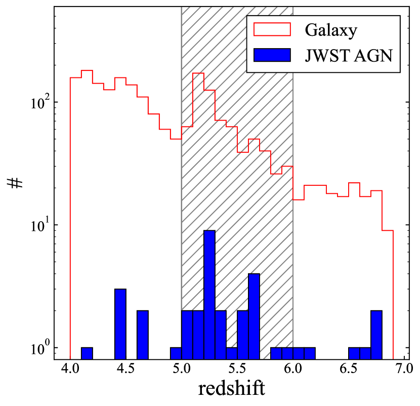
Figure 1: The redshift distribution based on spectroscopic redshifts of JWST AGNs (blue) and photometric redshirts of galaxies (red) samples in the compilation of the literature (Maiolino et al., 2023; Harikane et al., 2023; Kocevski et al., 2024; Matthee et al., 2024). The hatched region shows the galaxy and AGN samples utilised in this analysis.

Table 1: The effective area and the number of AGNs and galaxies in each field.

Field	Effective area	$N_{\mathrm{galaxy}}$	$N_{\mathrm{AGN}}$	Reference
	(arcmin2)	(#)	(#)
GOODS North	85.7	200	12	Maiolino et al. (2023); Matthee et al. (2024)
GOODS South	62.1	69	2	Maiolino et al. (2023); Matthee et al. (2024)
CEERS	95.3	207	12	Harikane et al. (2023); Kocevski et al. (2024)
PRIMER-UDS	166.2	203	2	Kocevski et al. (2024)
Total	409.3	679	28

3 Clustering Analysis

We first evaluate the angular cross-correlation function $\omega(\theta)$ in Section 3.1 taking into account that photometric redshift, whose uncertainty is larger than that of spectroscopic redshift, is only available for the galaxy sample. However, we note that the uncertainty of the photometric redshift is much smaller than the redshift range of the galaxy sample. We also evaluate the projected correlation function $\omega_{p}(r_{p})$ of each subsample in Section 3.2 to check the robustness of the result. We note that these measurements of the typical DMH mass are independent. We adopt almost the same way to evaluate the correlation functions in Arita et al. (2023); therefore we briefly describe the method.

3.1 Angular correlation function

We evaluate the angular cross-correlation function between JWST AGNs and galaxies, $\omega_{\mathrm{CCF}}(\theta)$, and the angular auto-correlation function of galaxies, $\omega_{\mathrm{ACF}}(\theta)$. We use the following estimators to evaluate the correlation functions (Landy & Szalay, 1993; Cooke et al., 2006):

$$\omega_{\mathrm{CCF}}(\theta) =\frac{D_{\mathrm{AGN}}D_{\mathrm{galaxy}}-D_{\mathrm{AGN}}R-D_{\mathrm{galaxy}}R+RR}{RR},$$ (4)

$$\omega_{\mathrm{ACF}}(\theta) =\frac{D_{\mathrm{galaxy}}D_{\mathrm{galaxy}}-2D_{\mathrm{galaxy}}R+RR}{RR},$$ (5)

where $D_{\mathrm{AGN}}D_{\mathrm{galaxy}},D_{\mathrm{AGN}}R,D_{\mathrm{galaxy}}R,RR,D_{\mathrm{galaxy}}D_{\mathrm{galaxy}}$ represent the normalised number of pairs between AGNs and galaxies, AGNs and random points, galaxies and random points, random points and random points, and galaxies and galaxies within the specified angular range, respectively. The random points are scattered over the survey region at a surface number density of 100 arcmin^-2. In order to trace the survey fields, we only use the random points located within $3\arcsec$ of objects with $n_{\mathrm{filter}}\geq 12$. We evaluate both cross- and auto-correlation functions at $\theta>10\arcsec$ to avoid the one-halo term. The uncertainties are estimated by the bootstrap resampling with $N=1000$ times iteration. We randomly select the same number of JWST AGNs and galaxies from the sample allowing duplication and evaluate the cross- and auto-correlation functions for each subsample. We calculate the covariance matrix below and the diagonal element shows the uncertainty of each bin:

$$C_{i,j}=\frac{1}{N-1}\sum_{k=1}^{N}(\omega_{i}^{k}-\overline{\omega}_{i})(\omega_{j}^{k}-\overline{\omega}_{j}),$$ (6)

where $\omega_{i}^{k}$ is the correlation function in $i$th bin of $k$th iteration and $\overline{\omega}_{i}$ shows the mean value of the correlation function in $i$th bin.

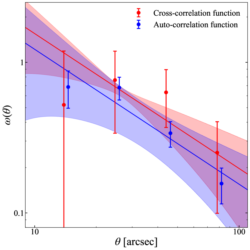
Figure 2: Angular correlation functions and the results of the MCMC fit (blue: auto-correlation function; red: cross-correlation function). The solid lines represent the best estimates of the power-law function $\omega(\theta)=(\theta/\theta_{0})^{-\beta}$ fitted to the correlation functions. The shaded region denotes the power-law functions with parameters in each MCMC step.

Figure 2 shows $\omega_{\mathrm{CCF}}$ (red) and $\omega_{\mathrm{ACF}}$ (blue). The red and blue solid lines show the best fit of a power-law function. Regarding the integral constraint due to the limited survey area (Groth & Peebles, 1977), we confirm that it can be negligible in a scale of $\theta\lesssim 100\arcsec$. Hence, we ignore the integral constraint in this analysis.

We use a Markov Chain Monte Carlo (MCMC) algorithm (Foreman-Mackey et al., 2013) to fit the simple power-law function, $\omega(\theta)=(\theta/\theta_{0})^{-\beta}$.We assume a Gaussian likelihood function and uniform priors for $\theta_{0}\in[1\arcsec,100\arcsec]$ and the slope $\beta\in[0,2]$. We define the best estimate as the median and 16th and 84th percentiles of the posterior distribution. First, we perform MCMC fit for the auto-correlation function because the signal-to-noise ratio is better than the cross-correlation function. We obtain $\theta_{0,\mathrm{ACF}}=11.\arcsec 90_{-2.79}^{+2.30}$ and $\beta=0.90_{-0.16}^{+0.16}$ as the best estimate. The cross-correlation function uses the same $\beta$ obtained in the MCMC fit to the auto-correlation function and evaluates $\theta_{0}$ for the fixed-$\beta$ in each MCMC step. Finally, we obtain $\theta_{0}$ for the cross-correlation function as $\theta_{0,\mathrm{CCF}}=16.\arcsec 33_{-2.00}^{+0.99}$.

The amplitude $A_{\omega}(=\theta_{0}^{\beta})$ can be converted into the correlation length, $r_{0}$ in physical scale. We calculate the correlation length of the cross-correlation function and the auto-correlation function by referring to Croom & Shanks (1999) and Limber (1953), respectively. We use the redshift distribution by kernel density estimation with Gaussian kernel based on Figure 1. Finally, we obtain $r_{0,\mathrm{CCF}}=6.68_{-0.78}^{+0.78}\,h^{-1}\mathrm{Mpc}$ and $r_{0,\mathrm{ACF}}=5.60_{-0.58}^{+0.59}\,h^{-1}\mathrm{Mpc}$. In this analysis, we do not take the contamination fraction into account because it hardly affects the estimation for DMH mass measurement of the JWST AGNs. The detail is described in Appendix A.

3.2 Projected correlation function

We also evaluate the projected cross-correlation function between JWST AGNs and galaxies, $\omega_{p,\mathrm{CCF}}(r_{p})$ and the projected auto-correlation function of galaxies, $\omega_{p,\mathrm{ACF}}(r_{p})$. The projected correlation functions are obtained by integrating the three-dimensional correlation functions, $\xi_{\mathrm{CCF}}(r_{p},\pi)$ and $\xi_{\mathrm{ACF}}(r_{p},\pi)$, where $r_{p}$ and $\pi$ represent the perpendicular and the parallel distances to the line-of-sight, respectively. While the redshifts of AGNs are determined spectroscopically, the galaxy sample only has the photometric redshifts. It should be noted that the uncertainty of photometric redshift, typically $\Delta z/(1+z)=0.026$, is larger than that of spectroscopic redshift, and this may make the actual uncertainty of the correlation functions a little larger. We adopt the following estimator to evaluate the three-dimensional correlation functions (Landy & Szalay, 1993; Cooke et al., 2006). Namely, the projected correlation functions can be evaluated as

$$\omega_{p,\mathrm{CCF/ACF}}(r_{p})=\int_{0}^{\pi_{\mathrm{cut}}}\xi_{\mathrm{CCF/ACF}}(r_{p},\pi)d\pi$$ (7)

where $\pi_{\mathrm{cut}}$ represents the optimum limit above which the clustering signal is almost negligible, which is fixed to $100\,h^{-1}\mathrm{Mpc}$, and

$$\xi_{\mathrm{CCF}}(r_{p},\pi)=$$

$$\frac{D_{\mathrm{AGN}}D_{\mathrm{galaxy}}-D_{\mathrm{AGN}}R_{\mathrm{galaxy}}-D_{\mathrm{galaxy}}R_{\mathrm{AGN}}+R_{\mathrm{AGN}}R_{\mathrm{galaxy}}}{R_{\mathrm{AGN}}R_{\mathrm{galaxy}}},$$ (8)

$$\xi_{\mathrm{ACF}}(r_{p},\pi)=\frac{D_{\mathrm{galaxy}}D_{\mathrm{galaxy}}-2D_{\mathrm{galaxy}}R_{\mathrm{galaxy}}+R_{\mathrm{galaxy}}R_{\mathrm{galaxy}}}{R_{\mathrm{galaxy}}R_{\mathrm{galaxy}}}.$$ (9)

In Equation (8) and (9), $D$ and $R$ represent data and random points, respectively, and the suffixes denote the population. The same random points in Section 3.1 are used, and their redshifts are assigned so as to reproduce the redshift distribution of the population shown in Figure 1. Each term shows the normalised pair count within a specified projected length range. The uncertainty of the projected correlation functions is estimated by the same method in Section 3.1. The covariance matrix is calculated by Equation (6) replacing $\omega$ for $\omega_{p}$.

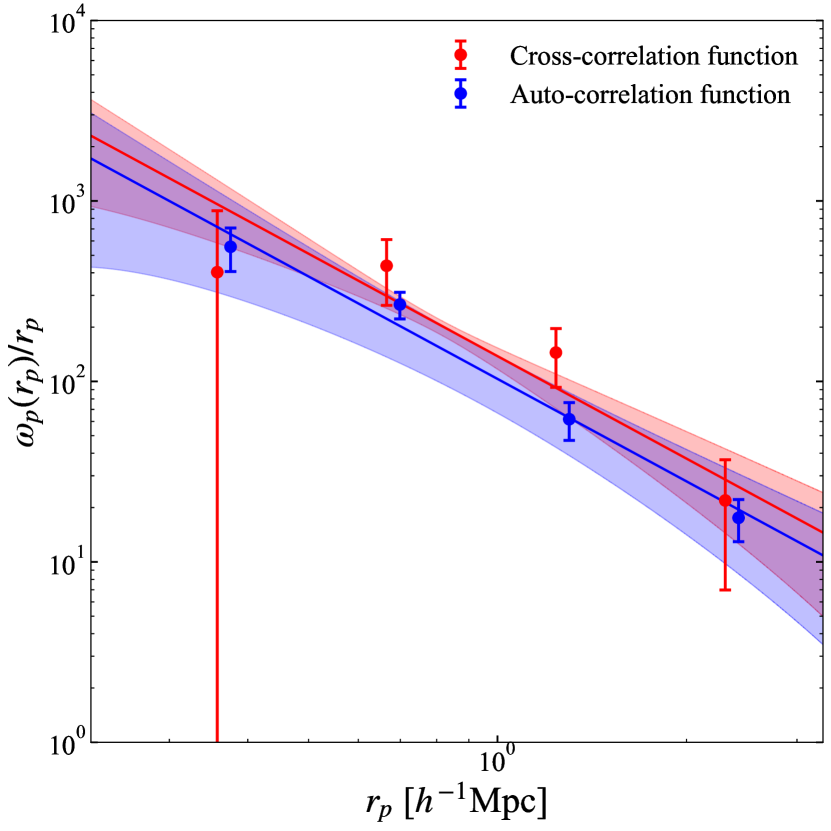
Figure 3: Projected correlation functions and the results of the MCMC power-law fit (blue: auto-correlation function; red: cross-correlation function). The solid lines represent the best estimates of Equation (11) fitted to the correlation functions. The shaded region denotes the power-law functions with parameters in each MCMC step.

Figure 3 shows the result of the projected correlation functions. The solid lines denote the power-law fit, which can be derived from the real-space correlation functions. The relation between projected correlation functions and real-space correlation functions $\xi(r)$ is described in Davis & Peebles (1983) as

$$\omega_{p}(r_{p})=2\int_{r_{p}}^{\infty}\frac{r\xi(r)}{\sqrt{r^{2}-r_{p}^{2}}}dr.$$ (10)

Assuming that the real-space correlation function is a power-law function expressed as $\xi(r)=(r/r_{0})^{-\gamma}$, the projected correlation function is represented as

$$\frac{\omega_{p}(r_{p})}{r_{p}}=H_{\gamma}\left(\frac{r_{p}}{r_{0}}\right)^{-\gamma},$$ (11)

where

$$H_{\gamma}=B\left(\frac{\gamma-1}{2},\frac{1}{2}\right)$$ (12)

in which $B$ is the beta function, and $r_{0}$ denotes the correlation length. We fit Equation (11) to the projected correlation function with the MCMC algorithm. Following Eilers et al. (2024), we assume a Gaussian likelihood function and uniform priors for the correlation length of $r_{0}\in[1,30]\,h^{-1}\mathrm{Mpc}$ and the slope of $\gamma\in[1,3]$. The best estimate is defined in the same manner in Section 3.1. Based on the MCMC fit for the auto-correlation function, we obtain $r_{0,\mathrm{ACF}}=5.80_{-0.62}^{+0.61}\,h^{-1}\mathrm{Mpc}$ and $\gamma=1.89_{-0.16}^{+0.16}$ as the best estimate. The same $\gamma$ is used in the MCMC fit for the cross-correlation function to evaluate the correlation length. Finally, we obtain the correlation length for the cross-correlation functions as $r_{0,\mathrm{CCF}}=7.11_{-0.83}^{+0.80}\,h^{-1}\mathrm{Mpc}$.

3.3 DMH mass of JWST AGNs

Based on the correlation lengths evaluated in Section 3.1 and 3.2, we evaluate the typical DMH mass of JWST AGNs. We assume that target objects are formed in the density peaks of underlying dark matter and trace the peaks (Sheth & Tormen, 1999). The correlation length can be converted into a bias parameter, which is defined as the ratio of clustering strength between objects and underlying dark matter at a scale of $8\,h^{-1}\mathrm{Mpc}$; therefore the bias parameter $b$ is obtained as

$$b=\sqrt{\frac{\xi(8,z)}{\xi_{\mathrm{DM}}(8,z)}},$$ (13)

where $\xi_{\mathrm{DM}}$ represents the correlation function of underlying dark matter. We utilise halomod(Murray et al., 2013, 2021) to calculate the denominator with the bias model of Tinker et al. (2010), the transfer function model of CAMB (Lewis & Challinor, 2011), and the growth model of Carroll et al. (1992). With regard to the numerator, we assume that $\xi(r)=(r/r_{0})^{-(1+\beta)}$ for the angular correlation function and $\xi(r)=(r/r_{0})^{-\gamma}$ for the projected correlation function with the correlation lengths obtained in Section 3. We derive the bias parameter $b_{\mathrm{CCF}}$ and $b_{\mathrm{galaxy}}$ from the cross- and auto-correlation functions with parameters in MCMC steps, which is utilised to evaluate the uncertainty. The bias parameters are summarised in Table 2. Finally, we estimate the bias parameter of JWST AGNs $b_{\mathrm{AGN}}$ from Mountrichas et al. (2009):

$$b_{\mathrm{CCF}}^{2}\sim b_{\mathrm{AGN}}b_{\mathrm{galaxy}}.$$ (14)

This equation yields $b_{\mathrm{AGN}}=6.97_{-1.06}^{+1.01}$ and $7.56_{-1.08}^{+0.97}$ from the angular and the projected correlation functions, respectively.

We convert the bias parameters of galaxies and JWST AGNs into the typical DMH mass in the same method as Arita et al. (2023). Finally, through the results in Section 3.1, we evaluate the typical DMH mass of the galaxies and JWST AGNs as $\log(M_{\mathrm{halo},\mathrm{AGN}}/h^{-1}\mathrm{M_{\odot}})=11.61_{-0.24}^{+0.19}$ and $\log(M_{\mathrm{halo},\mathrm{galaxy}}/h^{-1}\mathrm{M_{\odot}})=11.12_{-0.22}^{+0.18}$. Applying the results in Section 3.2 yields $\log(M_{\mathrm{halo},\mathrm{AGN}}/h^{-1}\mathrm{M_{\odot}})=11.72_{-0.20}^{+0.17}$ and $\log(M_{\mathrm{halo},\mathrm{galaxy}}/h^{-1}\mathrm{M_{\odot}})=11.18_{-0.22}^{+0.17}$, which are consistent with the results from angular correlation functions. In the evaluation of the typical DMH mass, we calculate the DMH masses for each bias from the parameters in MCMC steps and regard the median and 16th and 84th percentiles as the best estimate. The results including bias parameters are summarised in Table 2.

Table 2: Summary of the clustering analysis results. All of the uncertainty in this table is defined as median and 16th and 84th percentiles based on the MCMC fit.

Correlation function	$r_{0,\mathrm{ACF}}$	$r_{0,\mathrm{CCF}}$	$b_{\mathrm{galaxy}}$	$b_{\mathrm{CCF}}$	$b_{\mathrm{AGN}}$	$\log M_{\mathrm{halo},\mathrm{galaxy}}$	$\log M_{\mathrm{halo},\mathrm{AGN}}$
	$(h^{-1}\mathrm{Mpc})$	$(h^{-1}\mathrm{Mpc})$				$(h^{-1}\mathrm{M_{\odot}})$	$(h^{-1}\mathrm{M_{\odot}})$
Angular, $\omega(\theta)$	$5.60_{-0.58}^{+0.59}$	$6.68_{-0.78}^{+0.78}$	$5.01_{-0.64}^{+0.59}$	$5.67_{-0.77}^{+0.73}$	$6.97_{-1.06}^{+1.01}$	$11.12_{-0.22}^{+0.18}$	$11.61_{-0.24}^{+0.19}$
Projected, $\omega_{p}(r_{p})$	$5.80_{-0.62}^{+0.61}$	$7.11_{-0.83}^{+0.80}$	$5.20_{-0.66}^{+0.60}$	$6.19_{-0.86}^{+0.75}$	$7.56_{-1.08}^{+0.97}$	$11.18_{-0.22}^{+0.17}$	$11.72_{-0.20}^{+0.17}$

4 Discussion

4.1 Comparison of typical DMH mass of JWST AGNs and quasars

We compare the typical DMH mass of JWST AGNs with that of quasars derived by the clustering analysis. Figure 4 summarises the DMH mass measurement of quasars at $0\lesssim z\lesssim 6.5$ (Shen et al., 2007; Ross et al., 2009; Eftekharzadeh et al., 2015; He et al., 2018; Timlin et al., 2018; Arita et al., 2023; Eilers et al., 2024). The previous clustering analysis indicates that type-1 quasars have a nearly constant halo mass of $\log(M_{\mathrm{halo}}/h^{-1}\mathrm{M_{\odot}})\sim 12.5$ through the cosmic time (Trainor & Steidel, 2012; Shen et al., 2013; Timlin et al., 2018; Arita et al., 2023). Arita et al. (2023) discuss the possibility that there is a ubiquitous mechanism that activates quasars only in the DMHs with $12\lesssim\log(M_{\mathrm{halo}}/h^{-1}\mathrm{M_{\odot}})\lesssim 13$ (grey region in Figure 4). In contrast, the typical DMH mass of JWST AGNs is lower than theirs by $\sim 1$ dex, implying that JWST AGNs may be different populations than type-1 quasars. Pizzati et al. (2024b) predicts that the DMH mass of LRDs should be smaller than that of unobscured quasars from their large abundance difference. Although our sample is not necessarily identical to the LRDs, the DMH mass by the clustering analysis is consistent with the theoretical prediction. No examples of DMH masses as less massive as the JWST AGNs in this study have been measured even in the faint type-1 quasars at low-$z$. The DMH mass of JWST AGN is rather consistent with that of the galaxy sample within 1$\sigma$ errors. Given that they are different populations, there is no need for the abundance of the JWST AGNs on the luminosity function to coincide with the type-1 quasar’s extension to the faint-end, nor is there a need for the JWST AGN to follow the $M_{\mathrm{BH}}$-$M_{*}$ relation formed by the type-1 AGNs. However, since the lower limit of the mass range of typical quasars has not been rigorously measured, it is possible that faint quasars with $M_{1450}\gtrsim-20$ reside in less massive DMHs with $\log(M_{\mathrm{halo}}/h^{-1}\mathrm{M_{\odot}})<12$. Hence, the possibility that the JWST AGNs that are typically faint ($M_{1450}\gtrsim-20$) are new type-1 quasars hosted by less massive DMHs not previously found cannot be ruled out.

On the other hand, Allevato et al. (2014) reported that DMH mass of X-ray-selected type-2 AGNs at $z\sim 3$ is estimated as $\log(M_{\mathrm{halo}}/h^{-1}\mathrm{M_{\odot}})=11.73_{-0.45}^{+0.39}$, which is consistent with our measurements. However, there are contradicting measurements of DMH mass for type-2 AGNs. Allevato et al. (2011) showed that X-ray-selected narrow-line AGNs at $0.6\leq z\leq 1.5$ are hosted by massive DMHs with $\log(M_{\mathrm{halo}}/h^{-1}\mathrm{M_{\odot}})\sim 13.00\pm 0.06$. Viitanen et al. (2023) indicated that the DMH mass of X-ray-selected AGNs does not depend on their obsculation and that the typical DMH mass is $\log(M_{\mathrm{halo}}/h^{-1}\mathrm{M_{\odot}})=12.98_{-0.22}^{+0.17}(12.28_{-0.19}^{+0.13})$ at $z\sim 0.7(1.8)$. The DMH mass of JWST AGNs is less massive than that of X-ray selected AGNs (Krishnan et al., 2020) at $0<z<2.5$, hosted on average in DMHs of $10^{12\mathchar 45\relax 13}\,h^{-1}\mathrm{M_{\odot}}$.

We calculate the redshift evolution of the DMH mass of JWST AGNs based on the Extended Press-Schechter theory (e.g. Bower, 1991). The red and blue solid lines in Figure 4 show the evolution of the DMH mass with $\log(M_{\mathrm{halo}}/h^{-1}\mathrm{M_{\odot}})=11.61,11.72$ at $z=5.4$, respectively. We find that the DMHs hosting JWST AGNs grow to as massive as $\sim 10^{13}\,h^{-1}\mathrm{M_{\odot}}$ at $z=0$, which is comparable to the DMH mass of a galaxy cluster in the local Universe. Furthermore, we find that the DMH mass of JWST AGNs will reach $10^{12\mathchar 45\relax 13}\,h^{-1}\mathrm{M_{\odot}}$, a typical type-1 quasar’s DMH mass regime, at $z\lesssim 3$. This recalls a scenario where the JWST AGNs at $5<z<6$ will grow into quasars at $z\lesssim 3$. In other words, the JWST AGNs at $5<z<6$ are the ancestors of quasars at $z\lesssim 3$ and will start to shine as quasars in $\sim 1$ Gyr later. Here, from the perspective of DMH mass evolution, it can be reasonably explained that the DMH hosting the JWST AGN will grow to be comparable to the DMH at $z<3$ quasar, but please note that this does not guarantee that the JWST AGN will necessarily grow to be a quasar. According to Hopkins et al. (2008), an evolution model of quasars induced by a major merger, $\sim 1$ Gyr before a quasar phase corresponds to a coalescence phase. The model predicts that after the coalescence phase, a starburst occurs, significantly increasing the stellar mass of the host galaxy, and if this is correct, then at $z\sim 3$, the overmassive situation in JWST AGNs (Maiolino et al., 2023; Harikane et al., 2023) is supposed to be mitigated. The possibility of the episodic intense starburst for JWST AGNs is remarked in Kokorev et al. (2024a) based on their JWST observation for a LRD at $z=4.13$, which is consistent with the scenario. The details on the relation between the host stellar mass and the SMBH mass are discussed in Section 4.2.

Figure 4 also shows the typical DMH mass of our galaxy sample. The DMH mass of galaxies can also be inferred by combining their stellar mass, which is estimated by EAZY in the DJA catalogue, and the empirical stellar-to-halo mass ratio of Behroozi et al. (2019). Dividing the stellar mass of the individual galaxies by the stellar-to-halo mass ratio yields $\log(\overline{M}_{\mathrm{halo},\mathrm{galaxy}}/h^{-1}\mathrm{M_{\odot}})=11.40_{-0.25}^{+0.26}$ as the median DMH mass of the galaxies, which is consistent with the DMH mass measured by the clustering analysis. The consistency supports the robustness of the clustering analysis.

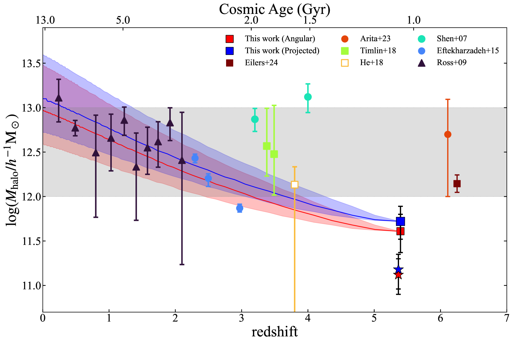
Figure 4: Comparison of DMH mass of JWST AGNs in this study (blue square: angular, red square: projected) with those in literature based on the clustering analysis. We also show the DMH mass of galaxies as stars. The symbols of previous studies are classified by type of correlation function (circle: projected correlation function, square: angular correlation function, triangle: redshift-space correlation function). The filled and open symbols show the auto-correlation function and the cross-correlation function is used to estimate the typical DMH mass. We note that the DMH masses in the previous studies have been converted to those using cosmological parameters in this study and their bias parameters, because some cosmological parameters, particularly $\sigma_{8}$, have a large impact on the DMH mass estimate. The grey-shaded region shows the typical DMH mass range of quasars suggested by Trainor & Steidel (2012); Shen et al. (2013); Timlin et al. (2018); Arita et al. (2023). The solid lines with the shaded regions denote the mass evolution of DMH hosting JWST AGNs at $5<z<6$ and its $1\sigma$ error calculated by the extended Press-Schechter theory.

4.2 Host stellar mass of JWST AGNs

The host stellar mass of JWST AGNs can be inferred by the empirical relation between the stellar mass and DMH mass of galaxies (Behroozi et al., 2019). We multiply the typical DMH mass of JWST AGNs by the stellar-to-halo mass ratio at $z\sim 5.4$ to obtain the host stellar mass of JWST AGNs as $\log(M_{*}/\mathrm{M_{\odot}})=9.72_{-0.39}^{+0.31}$ and $9.90_{-0.33}^{+0.27}$ from the angular and the projected correlation functions, respectively. Our results are consistent with the stellar mass estimates for LRD candidates at $5<z<6$ in COSMOS-Web regions by SED fitting with NIRCam and MIRI photometry (Akins et al., 2024). However, they are slightly higher than the estimate in Harikane et al. (2023) and $\gtrsim 1$ dex higher than the stellar mass estimated individually in Maiolino et al. (2023). Harikane et al. (2023) executed AGN decomposition before SED fitting, while Maiolino et al. (2023) performed SED fitting by BEAGLE (Chevallard & Charlot, 2016) with the AGN and the galaxy components to estimate the stellar mass. Maiolino et al. (2023) remark that some of the estimated stellar masses are significantly smaller than the inferred dynamical mass, implying that their stellar mass might be underestimated due to the difficulty in assessing the AGN contribution. In addition, Casey et al. (2024) suggested that the stellar mass of LRDs is smaller than those obtained by the SED fitting when applying the maximum star-to-dust ratio (Schneider & Maiolino, 2024). However, it remains to be elucidated whether the general star-to-dust ratio and the stellar-to-halo mass ratio can apply to the JWST AGNs.

Figure 5 compares the average $M_{*}$-$M_{\mathrm{BH}}$ relation for the JWST AGNs in this analysis and those in the literature. The $M_{\mathrm{BH}}$ of the individual JWST AGNs has been measured based on the FWHM of broad H$\alpha$ emission and the luminosity (e.g. Greene & Ho, 2005; Reines et al., 2013; Reines & Volonteri, 2015), and we use the median mass of 28 JWST AGNs to evaluate the median $M_{\mathrm{BH}}/M_{*}$ in this study. Figure 5 also displays the local relation (Reines & Volonteri, 2015) and high-$z$ relation (Pacucci et al., 2023), which is based on the JWST AGNs at $4<z<7$. While Maiolino et al. (2023) and Harikane et al. (2023) reported that JWST AGNs have highly overmassive SMBHs (grey circles in Figure 5), our estimate shows the trend is much less pronounced. Our results fall between the JWST AGNs’ relation (Pacucci et al., 2023) and the local AGN relation (Reines & Volonteri, 2015). Our results are rather consistent with Sun et al. (2024), who insist that $M_{\mathrm{BH}}/M_{*}$ shows no redshift evolution up to $z=4$.

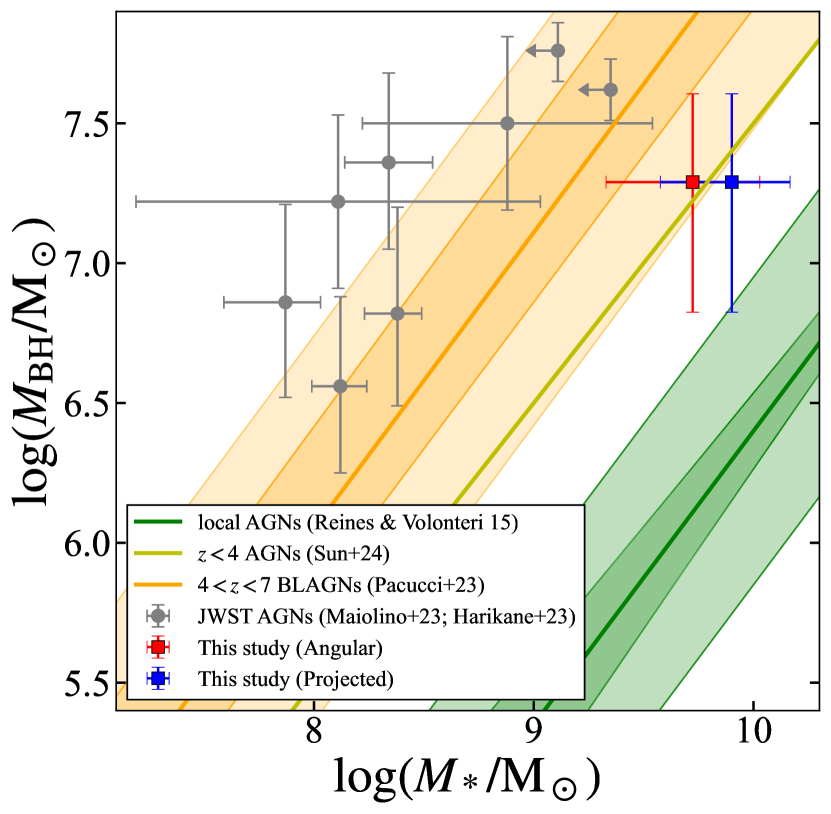
Figure 5: The relation between stellar mass and SMBH mass of JWST AGNs. The median stellar mass evaluated based on the DMH mass and the empirical stellar-to-halo mass ratio in this study is shown as red and blue squares. The grey points show the stellar mass and SMBH mass of individual JWST AGNs (Maiolino et al., 2023; Harikane et al., 2023). The green line denotes the relation of local AGNs (Reines & Volonteri, 2015). The orange line represents the relation based on the broad-line AGNs (BLAGNs) at $4<z<7$ identified by JWST (Pacucci et al., 2023). The deep and light-shaded regions show the $1\sigma$ error and the intrinsic scatter, respectively. The yellow line is the high-$z$ ($z<4$) relation suggested by Sun et al. (2024).

We also estimate a possible evolution of the $M_{*}$-$M_{\mathrm{BH}}$ relation for JWST AGNs. We adopt the black hole accretion rate (BHAR) of TRINITY (Zhang et al., 2023), which provides the average BHAR as a function of redshift and the DMH mass. TRINITY utilises a halo merger tree and scaling relations among DMHs, galaxies, and SMBHs to predict the masses of DMHs, galaxies, and SMBHs at each redshift bin. The BHAR can be obtained from the time derivative of the SMBH masses. We simply assume that the host galaxies of JWST AGNs have a constant star formation rate (SFR). We estimate the total SFR by summing the SFRs derived by the H$\alpha$ luminosity in the narrow line component (Matthee et al., 2024) and that from the IR luminosity (Casey et al., 2024). Matthee et al. (2024) adopt Kennicutt & Evans (2012) to estimate SFR from the H$\alpha$ luminosity as $15\,\mathrm{M_{\odot}}\mathrm{yr^{-1}}$. Casey et al. (2024) inferred the mean IR luminosity of LRDs as $\langle L_{\mathrm{IR}}\rangle=(7.9_{-4.7}^{+2.9})\times 10^{10}\,\mathrm{L_{\odot}}$, which yields $\mathrm{SFR_{IR}}\sim 10\,\mathrm{\mathrm{M_{\odot}}\,yr^{-1}}$ by applying the empirical relation (Kennicutt & Evans, 2012). Finally, we assume the SFR of JWST AGNs as time-invariant with $25\,\mathrm{\mathrm{M_{\odot}}\,yr^{-1}}$. Please note that there is a great deal of uncertainty involved in estimating SFR. If we stand on the model of Hopkins et al. (2008) mentioned in Section 3.3, JWST AGN may undergo a starburst in the future, so this assumption may be an underestimate. Figure 6 shows the evolution paths of $M_{\mathrm{BH}}/M_{*}$. We confirm that most of the JWST AGNs will follow the low-$z$ relation (Sun et al., 2024) at $z\lesssim 3$, which supports the hypothesis that the JWST AGNs at $5<z<6$ are the ancestors of quasars at $z\lesssim 3$. TRINITY predicts that AGNs residing in DMHs with $M_{\mathrm{halo},z=0}=10^{13}\,h^{-1}\mathrm{M_{\odot}}$ will remain low in BHAR from $z\sim 5$ to $z\sim 3$, which helps mitigate the offset to the local relation at $z<3$. In addition, TRINITY also predicts that the BHAR will start to increase at $z\sim 3$, which implies that the AGNs become active at $z\sim 3$. Furthermore, recent JWST observation (Kokorev et al., 2024b) for an LRD at $z=4.13$ shows a consistent $M_{\mathrm{BH}}$-$M_{*}$ relation with local one (Kormendy & Ho, 2013; Greene et al., 2016, 2020). They suggest that a starburst may occur after forming an overmassive SMBH at high-$z$ and the $M_{\mathrm{BH}}/M_{*}$ gets closer to the local relation. Although this differs from the assumed star formation history, the final fate of JWST AGNs is the same as the conclusion of this study. The above assessment assumes that all JWST AGNs have an average DMH mass; however, individual JWST AGNs should have different DMH masses and therefore different BHARs. Zhang et al. (2024) also predicts the redshift evolution of $M_{\mathrm{BH}}/M_{*}$ of JWST AGNs at $z\gtrsim 4$. Their calculation shows that $M_{\mathrm{BH}}/M_{*}$ will keep almost constant or slightly increase toward $z=0$, which suggests that JWST AGNs are still overmassive even at $z=0$, though no such population has been found. The result may be due to the fact that they assume mathematically that all SMBHs with the same host stellar mass share the same average Eddington ratio distribution. As such, the prediction of $M_{\mathrm{BH}}/M_{*}$ of JWST AGNs has a large variation among individual studies with different assumptions.

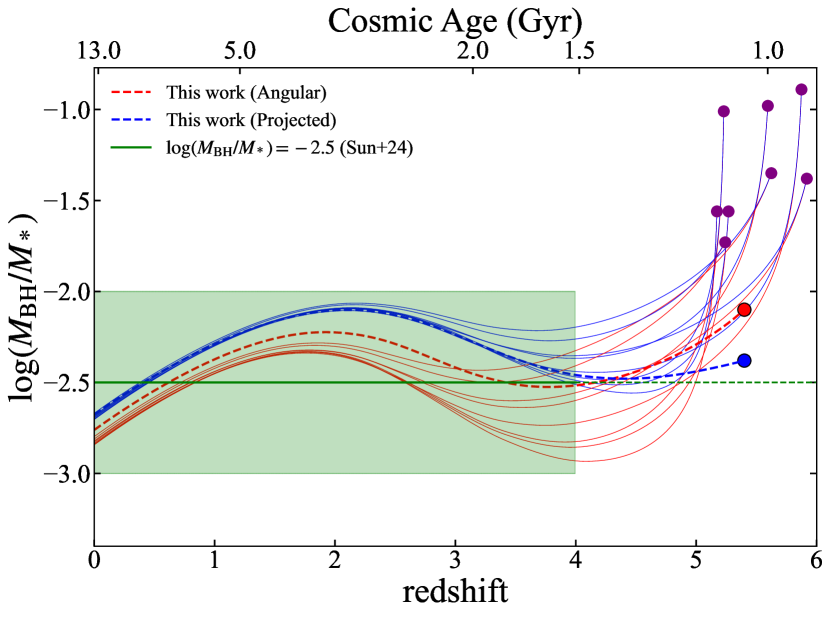
Figure 6: The redshift evolution of $M_{\mathrm{BH}}/M_{*}$. The red and blue dashed lines represent the evolution based on the angular and the projected correlation function. The solid lines show the evolution of individual JWST AGNs whose stellar mass is estimated in the literature (Maiolino et al., 2023; Harikane et al., 2023). Their initial $M_{\mathrm{BH}}/M_{*}$ is represented as purple circles. The red and blue ones calculate the BHAR based on the DMH mass evolution of the angular and the projected correlation functions. The green line denotes $M_{\mathrm{BH}}/M_{*}=-2.5$ at $z<4$ (Sun et al., 2024) and the green-shaded region displays a scatter of 0.5 dex.

4.3 Duty cycle

The duty cycle of AGNs, $f_{\mathrm{duty}}$, is defined as the time fraction of their active phase in the cosmic age. Although numerous assumptions are needed to infer the duty cycle, we estimate it based on the DMHs of JWST AGNs derived by the clustering analysis. In order to estimate the duty cycle of JWST AGNs, we assume that a DMH with $M_{\mathrm{halo,min}}\leq M_{\mathrm{halo}}\leq M_{\mathrm{halo,max}}$ hosts a JWST AGN and that JWST AGNs shines randomly in time. Based on the assumption, the duty cycle can be derived as

$$f_{\mathrm{duty}}=\frac{\int_{L_{\mathrm{min}}}^{L_{\mathrm{max}}}\Phi(L)\,dL}{\int_{M_{\mathrm{halo,min}}}^{M_{\mathrm{halo,max}}}n(M)dM},$$ (15)

where $L_{\mathrm{min}}$ and $L_{\mathrm{max}}$ are the minimum and maximum luminosity of JWST AGNs used in the clustering analysis, respectively. $\Phi(L)$ represents the luminosity function of JWST AGNs, and $n(M)$ denotes the DMH mass function. Although it is under discussion which functions (e.g.double power-law, Schechter, or else) are appropriate to describe as the LF of JWST AGNs, we refer to the LF derived in Matthee et al. (2024) and average the values at $M_{\mathrm{UV}}=-18.0,-19.0,-20.0$ to obtain $\log(\Phi(M_{\mathrm{UV}})/\mathrm{Mpc^{-3}\,mag^{-1}})=-4.94_{-0.22}^{+0.18}$. We assume $M_{\mathrm{halo,min}}$ and $M_{\mathrm{halo,max}}$ as $10^{11}\,h^{-1}\mathrm{M_{\odot}}$ and $10^{12}\,h^{-1}\mathrm{M_{\odot}}$, respectively, which covers our DMH mass estimates. The mass range is arbitrarily determined, and it is undeniable that the duty cycle significantly changes depending on how this range is taken. It should be noted that even if we apply the usual definition of duty cycle (e.g. Eftekharzadeh et al., 2015; He et al., 2018) with $M_{\mathrm{halo,max}}$ replaced by $\infty$, the resulting value of $f_{\mathrm{duty}}$ does not change significantly. We adopt the DMH mass function of Sheth & Tormen (1999). Finally, we obtain $f_{\mathrm{duty}}=0.36_{-0.14}^{+0.18}$ per cent, which implies the lifetime of $4\times 10^{6}$ yr for JWST AGNs at $5<z<6$, which is comparable to that of type-1 quasars at $z\lesssim 3$ (White et al., 2012; Eftekharzadeh et al., 2015; Laurent et al., 2017). This result also supports the scenario that JWST AGNs are the ancestors of quasars at $z\lesssim 3$. If the DMH mass of JWST AGN is as massive as that of quasars, namely $M_{\mathrm{halo,min}}=10^{12}\,h^{-1}\mathrm{M_{\odot}}$, the duty cycle would be larger than unity. This means that all of the massive DMHs host type-1 AGNs, and consequently this case does not allow inactive SMBHs and type-2 AGNs to reside in massive DMHs at $5<z<6$. Thus, it is qualitatively inferred that JWST AGNs reside in less massive DMHs than quasars. The duty cycle of $0.36_{-0.14}^{+0.18}$ per cent obtained here is self-consistent with the results that the typical DMH mass of JWST AGNs is less massive than that of quasars, as long as AGN activity is considered to be a transient phenomenon in the host galaxy.

Figure 7 compares the duty cycle of JWST AGNs $f_{\mathrm{duty,\,JWST\,AGNs}}$ with those of quasars $f_{\mathrm{duty,\,quasars}}$. Some of the quasar duty cycles are estimated based on the clustering analysis by estimating the minimum DMH mass to host a quasar (Shen et al., 2007; White et al., 2012; Eftekharzadeh et al., 2015; Laurent et al., 2017; Eilers et al., 2024). Pizzati et al. (2024a) and Pizzati et al. (2024c) also utilise the clustering analysis, and they evaluate the mass function of DMH hosting a quasar to measure the quasar duty cycle with dark matter-only simulation. Other studies estimate the duty cycle based on the Ly$\alpha$ damping wings of quasar spectra (Davies et al., 2019; Ďurovčíková et al., 2024). We find that the duty cycle of JWST AGNs is comparable to that of quasars at $z<5$ while it is slightly higher than that of quasars at $z>6$.

However, we caution that the estimated duty cycle of the JWST AGNs has a large uncertainty. It is difficult to determine the mass range of DMHs hosting JWST AGNs, and their luminosity function has a large variation among the literature. These uncertainties are inevitable for the estimate of the duty cycle using the method adopted in this study.

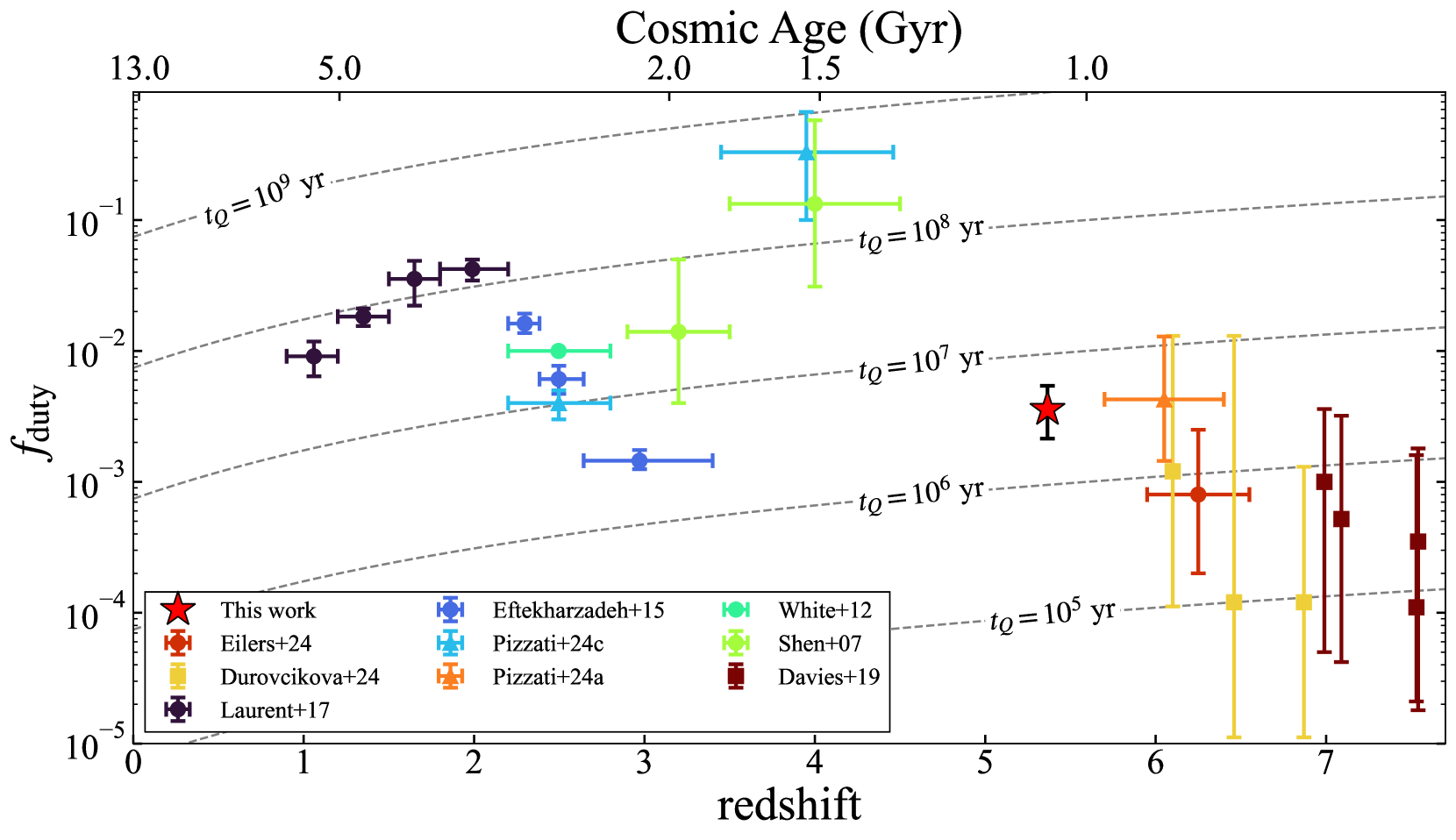
Figure 7: Duty cycle of quasars and JWST AGNs. Our result is plotted as a red star. The markers of previous studies show which method is adopted to estimate the duty cycle of quasars (circle: clustering analysis, square: Ly$\mathrm{\alpha}$ damping wing: triangle: cosmological simulation with clustering analysis). The dashed lines show $t_{Q}=10^{5},10^{6},10^{7},10^{8},10^{9}$ yr, where $t_{Q}$ represents the quasar lifetime.

4.4 The Nature of JWST AGNs

We discuss possible interpretations of JWST AGNs based on the DMH mass, host stellar mass, and the duty cycle estimated in this study. We suggest four possibilities on the nature of JWST AGNs: (a) ancestors of the low-$z$ quasars; (b) a new AGN population; (c) low-DMH-mass type-1 quasars; (d) non-AGN objects.

1. Ancestors of the low-$z$ quasars: As described in Section 4.1, DMHs that host JWST AGNs will grow to $10^{12\mathchar 45\relax 13}\,h^{-1}\mathrm{M_{\odot}}$, a typical DMH mass range of quasars (Trainor & Steidel, 2012; Shen et al., 2013; Timlin et al., 2018; Arita et al., 2023) at $z\lesssim 3$. This interpretation is compatible with the scenario suggested by Hopkins et al. (2008). The JWST AGN sees a period of coalescence with significant host stellar mass growth, after which the SMBH mass rapidly increases and the AGN enters the quasar phase after $\sim 1$ Gyr. The $M_{\mathrm{BH}}/M_{*}$, which is overmassive at $z\sim 5.5$, is also found to become consistent with the local AGN value at $z<4$ (Sun et al., 2024). JWST AGN does not need to continue to be active until it becomes a quasar, and this is consistent with the evaluation in this study that the duty cycle is less than unity. However, we caution that significant uncertainties about the evolution of SFR and BHAR are inevitable. The fact that most of the JWST AGNs are non-detectable in X-ray can be explained if we consider that their BHARs are already declining. In addition, if JWST AGNs see a period of coalescence, their H$\alpha$ luminosity should be enhanced, which can easily explain the deviation from the relation between X-ray luminosity and H$\alpha$ luminosity (Yue et al., 2024). If JWST AGNs are precursors to quasars, then similar objects could be found at any epoch in the universe. It would be interesting to find such objects in the low-$z$ universe (Juodžbalis et al., 2024).

2. A new AGN population: At $5<z<6$, the typical DMH mass of JWST AGNs is $\sim 1$ dex smaller than that of quasars. This difference suggests that JWST AGNs and quasars may be a different population. For instance, Maiolino et al. (2024) proposed that the X-ray emission of the JWST AGNs is intrinsically weak. They suggested a narrow-line Seyfert 1 with a high accretion rate and AGNs without hot corona as possible scenarios. It is necessary to understand the detailed mechanism of X-ray weakness and the lack of flux variability observed in JWST AGNs. Since JWST AGNs are considered to be a different population from what we call type-1 AGNs, their LFs do not need to be loosely connected to each other, and their contribution to reionization should be considered independently based on the different escape fraction of ionizing photons, which means that the JWST AGNs’ contribution is not necessarily the same as that of the type-1 AGNs’ contribution.

3. Low-DMH-mass type-1 quasars: This study shows that the DMH mass of JWST AGN is smaller than that of typical type-1 quasars, but this does not completely rule out that JWST AGN is a type-1 quasar. The typical DMH mass range of quasars is suggested to be constant $12\lesssim\log(M_{\mathrm{halo}}/h^{-1}\mathrm{M_{\odot}})\lesssim 13$ across most of the cosmic time, but this DMH mass range is not rigorously measured, and it is not surprising that lower-DMH-mass type-1 quasars exist. In fact, Pizzati et al. (2024a) predicts broader distribution of host halo masses. However, it is curious that no such low-DMH-mass type-1 quasars have been found in the nearby universe. This scenario most easily explains the observed broad Balmer lines, but of course, it continues to suffer from the previously noted problems of X-ray weakness and lack of flux variability in the JWST AGN.

4. Non-AGN objects: Since the DMH mass of the JWST AGNs is found to deviate from those of typical type-1 AGNs and it is closer to that of bright galaxies, it is also viable that they are non-AGN objects. In this case, the calculation of the duty cycle in Section 4.3 should be reconsidered. Some features remain to be elucidated to determine whether JWST AGNs are classified as AGNs. One of the features is the lack of flux variability reported in Kokubo & Harikane (2024). They suggested that the broad Balmer lines may not originate from broad line regions in AGNs but from the ultrafast outflow or Hi Raman scattering (but see Juodžbalis et al., 2024). Another feature is the weak X-ray emission (Yue et al., 2024; Maiolino et al., 2024). In addition, Baggen et al. (2024) suggested that some of the broad Balmer lines in LRDs may not need AGN contribution by reflecting the kinematics of the host galaxies. They find that stellar density in the centre of several LRDs is extremely high, and therefore the velocity dispersion is also large (see also Guia et al., 2024). Thus, we caution that a detailed observation is needed to conclude whether the broad line components originate from AGNs or not.

5 Summary

In this paper, we conduct the clustering analysis to evaluate the typical DMH mass of low-luminosity AGNs newly identified by JWST. We compile literature to select 28 AGNs at $5<z<6$ whose broad Balmer lines have been detected by JWST and select 679 galaxies in the same fields over $409.3\,\mathrm{arcmin^{2}}$ from the public galaxy catalogue. The main results are summarised below.

1. The angular and the projected cross-correlation functions yield $\log(M_{\mathrm{halo}}/h^{-1}\mathrm{M_{\odot}})=11.61_{-0.24}^{+0.19},11.72_{-0.20}^{+0.17}$, respectively, which are $\sim 1$ dex smaller than the typical DMH mass of quasars at $0<z<6$ derived by the clustering analysis.

2. The DMH mass evolution based on the extended Press-Schechter theory suggests that the DMHs of JWST AGNs at $5<z<6$ will grow to $10^{12\mathchar 45\relax 13}\,h^{-1}\mathrm{M_{\odot}}$, a typical mass of quasar at $z\lesssim 3$, implying that JWST AGNs are ancestors of the quasars at $z\lesssim 3$.

3. The host stellar mass of JWST AGNs is evaluated as $\log(M_{*}/\mathrm{M_{\odot}})=9.72_{-0.39}^{+0.31}$ and $9.90_{-0.33}^{+0.27}$ based on the measured DMH mass and the empirical stellar-to-halo mass ratio (Behroozi et al., 2019). The mass is consistent with the inferred stellar mass in Akins et al. (2024), who performed SED fitting with NIRCam and MIRI photometry, while it is higher than the estimate by SED fitting after decomposing the AGNs in Harikane et al. (2023) and Maiolino et al. (2023).

4. Assuming that JWST AGNs are the ancestor of $z<3$ quasars, it is speculated that SMBH-overmassive JWST AGNs will experience a starburst later stage based on the model of Hopkins et al. (2008), and approach the local $M_{\mathrm{BH}}$-$M_{*}$ relation. We calculate the possible evolution of $M_{\mathrm{BH}}/M_{*}$ assuming the BHAR of TRINITY and constant SFR of $25\,\mathrm{M_{\odot}}\,\mathrm{yr}^{-1}$. We find that the JWST AGNs will become consistent with the local relation of Sun et al. (2024) at $z\lesssim 3$ while they are overmassive at $5<z<6$.

5. We evaluate the duty cycle assuming that a DMH with $11\leq\log(M_{\mathrm{halo}}/h^{-1}\mathrm{M_{\odot}})\leq 12$ can host a JWST AGN and they shine in a certain period randomly. We obtain the duty cycle of JWST AGNs as $f_{\mathrm{duty}}=0.36_{-0.14}^{+0.18}$ per cent, which corresponds to the lifetime of $\sim 4\times 10^{6}\,\mathrm{yr}$. The duty cycle is comparable to that of quasars at $z<4$, while it is $\sim 1\mathchar 45\relax 2$ dex higher than that of quasars at $z\sim 6$.

6. Based on the DMH mass measured in this paper along with other observational properties, we argue the following four possibilities: (a) ancestors of quasars at $z\lesssim 3$; (b) a different AGN population from type-1 AGNs. We cannot exclude the other possibilities that (c) JWST AGNs are merely low-mass type-1 quasars or (d) non-AGN objects.

Future JWST observations with NIR Spec IFU will reveal the AGN-driven outflow and the chemical enrichment of the host galaxies, which will provide important hints for understanding the nature of the JWST AGNs. However, JWST AGNs, especially LRDs, are not observable in various wavelengths, which implies that other approaches are important to understand their nature. In this paper, we have shown that clustering analysis and the derived DMH mass provide a useful clue for examining the connection between the newly discovered JWST AGN and the previously known population. For further analysis, it is necessary to enlarge the sample size of spectroscopically confirmed JWST AGNs and detect them uniformly in the field of view. The observations will enable us to evaluate the three-dimensional correlation function and the auto-correlation function of JWST AGNs, which may allow us to more precisely evaluate the DMH mass. They will have an immense impact on our understanding of the JWST AGNs.

Data Availability

The JWST AGN data and galaxy data were obtained from the literature and DJA, both of which are open to the public. The derived data generated in this research will be shared on reasonable requests to the corresponding author.

Appendix A Correction of contamination

While the JWST AGNs are detected spectroscopically, the galaxies are selected based on photometric redshift, which will cause contamination in the galaxy sample and the rate should be taken into consideration. We simply assume that contaminating objects are randomly distributed over the survey area. In this case, the amplitudes of cross- and auto-correlation functions can be corrected as

$$A^{\prime}_{\omega,\mathrm{CCF}} =\frac{A_{\omega,\mathrm{CCF}}}{1-f_{c}^{\mathrm{galaxy}}},$$ (16)

$$A^{\prime}_{\omega,\mathrm{ACF}} =\frac{A_{\omega,\mathrm{ACF}}}{(1-f_{c}^{\mathrm{galaxy}})^{2}},$$ (17)

where $f_{c}^{\mathrm{galaxy}}$ is the fraction of contaminating sources in the galaxy sample (He et al., 2018). As shown in the Limber’s equation (Limber, 1953) and (13), we obtain the following relation between the bias parameter and the amplitude:

$$b\propto r_{0}^{\gamma/2}\propto\sqrt{A}.$$ (18)

Then, adopting the relation to Equation (14) and assuming that the contaminating sources have little effect on the photometric redshift distribution or the contamination fraction is small, the following relation is derived:

$$b_{\mathrm{AGN}}\sim\frac{b_{\mathrm{CCF}}^{2}}{b_{\mathrm{galaxy}}}\propto\sqrt{\frac{A_{\omega,\mathrm{CCF}}^{2}}{A_{\omega,\mathrm{ACF}}}}.$$ (19)

Combining the equation with Equation (16) and (17) yields

$$\sqrt{\frac{A_{\omega,\mathrm{CCF}}^{2}}{A_{\omega,\mathrm{ACF}}}}=\sqrt{\frac{{A^{{}^{\prime}2}_{\omega,\mathrm{CCF}}}}{{A}^{\prime}_{\omega,\mathrm{ACF}}}},$$ (20)

which demonstrates that the contamination fraction does not affect the bias parameter of JWST AGNs.

References

- Adelberger et al. (2006) Adelberger K. L., Steidel C. C., Kollmeier J. A., Reddy N. A., 2006, ApJ, 637, 74
- Akins et al. (2024) Akins H. B., et al., 2024, arXiv e-prints, p. arXiv:2406.10341
- Allevato et al. (2011) Allevato V., et al., 2011, ApJ, 736, 99
- Allevato et al. (2014) Allevato V., et al., 2014, ApJ, 796, 4
- Arita et al. (2023) Arita J., et al., 2023, ApJ, 954, 210
- Bañados et al. (2018) Bañados E., et al., 2018, Nature, 553, 473
- Baggen et al. (2024) Baggen J. F. W., et al., 2024, arXiv e-prints, p. arXiv:2408.07745
- Barro et al. (2024) Barro G., et al., 2024, ApJ, 963, 128
- Behroozi et al. (2019) Behroozi P., Wechsler R. H., Hearin A. P., Conroy C., 2019, MNRAS, 488, 3143
- Boutsia et al. (2021) Boutsia K., et al., 2021, ApJ, 912, 111
- Bower (1991) Bower R. G., 1991, MNRAS, 248, 332
- Brammer (2023a) Brammer G., 2023a, grizli, doi:10.5281/zenodo.7712834
- Brammer (2023b) Brammer G., 2023b, msaexp: NIRSpec analyis tools, doi:10.5281/zenodo.7299500
- Brammer et al. (2008) Brammer G. B., van Dokkum P. G., Coppi P., 2008, ApJ, 686, 1503
- Carroll et al. (1992) Carroll S. M., Press W. H., Turner E. L., 1992, ARA&A, 30, 499
- Casey et al. (2024) Casey C. M., Akins H. B., Kokorev V., McKinney J., Cooper O. R., Long A. S., Franco M., Manning S. M., 2024, arXiv e-prints, p. arXiv:2407.05094
- Chevallard & Charlot (2016) Chevallard J., Charlot S., 2016, MNRAS, 462, 1415
- Cooke et al. (2006) Cooke J., Wolfe A. M., Gawiser E., Prochaska J. X., 2006, ApJ, 652, 994
- Croom & Shanks (1999) Croom S. M., Shanks T., 1999, MNRAS, 307, L17
- Croom et al. (2005) Croom S. M., et al., 2005, MNRAS, 356, 415
- Davies et al. (2019) Davies F. B., Hennawi J. F., Eilers A.-C., 2019, ApJ, 884, L19
- Davis & Peebles (1983) Davis M., Peebles P. J. E., 1983, ApJ, 267, 465
- Dickinson et al. (2003) Dickinson M., Giavalisco M., GOODS Team 2003, in Bender R., Renzini A., eds, The Mass of Galaxies at Low and High Redshift. p. 324 (arXiv:astro-ph/0204213), doi:10.1007/10899892_78
- Dunlop et al. (2021) Dunlop J. S., et al., 2021, PRIMER: Public Release IMaging for Extragalactic Research, JWST Proposal. Cycle 1, ID. #1837
- Eftekharzadeh et al. (2015) Eftekharzadeh S., et al., 2015, MNRAS, 453, 2779
- Eilers et al. (2024) Eilers A.-C., et al., 2024, arXiv e-prints, p. arXiv:2403.07986
- Eisenstein et al. (2023) Eisenstein D. J., et al., 2023, arXiv e-prints, p. arXiv:2306.02465
- Finkelstein et al. (2019) Finkelstein S. L., et al., 2019, ApJ, 879, 36
- Finkelstein et al. (2023) Finkelstein S. L., et al., 2023, ApJ, 946, L13
- Foreman-Mackey et al. (2013) Foreman-Mackey D., Hogg D. W., Lang D., Goodman J., 2013, PASP, 125, 306
- Giallongo et al. (2015) Giallongo E., et al., 2015, A&A, 578, A83
- Giallongo et al. (2019) Giallongo E., et al., 2019, ApJ, 884, 19
- Grazian et al. (2022) Grazian A., et al., 2022, ApJ, 924, 62
- Greene & Ho (2005) Greene J. E., Ho L. C., 2005, ApJ, 630, 122
- Greene et al. (2016) Greene J. E., et al., 2016, ApJ, 826, L32
- Greene et al. (2020) Greene J. E., Strader J., Ho L. C., 2020, ARA&A, 58, 257
- Greene et al. (2024) Greene J. E., et al., 2024, ApJ, 964, 39
- Groth & Peebles (1977) Groth E. J., Peebles P. J. E., 1977, ApJ, 217, 385
- Guia et al. (2024) Guia C. A., Pacucci F., Kocevski D. D., 2024, Research Notes of the American Astronomical Society, 8, 207
- Harikane et al. (2023) Harikane Y., et al., 2023, ApJ, 959, 39
- He et al. (2018) He W., et al., 2018, PASJ, 70, S33
- Hickox et al. (2011) Hickox R. C., et al., 2011, ApJ, 731, 117
- Hopkins et al. (2008) Hopkins P. F., Hernquist L., Cox T. J., Kereš D., 2008, ApJS, 175, 356
- Juodžbalis et al. (2024) Juodžbalis I., et al., 2024, arXiv e-prints, p. arXiv:2407.08643
- Kashino et al. (2023) Kashino D., Lilly S. J., Matthee J., Eilers A.-C., Mackenzie R., Bordoloi R., Simcoe R. A., 2023, ApJ, 950, 66
- Kennicutt & Evans (2012) Kennicutt R. C., Evans N. J., 2012, ARA&A, 50, 531
- Kocevski et al. (2023) Kocevski D. D., et al., 2023, ApJ, 954, L4
- Kocevski et al. (2024) Kocevski D. D., et al., 2024, arXiv e-prints, p. arXiv:2404.03576
- Kokorev et al. (2023) Kokorev V., et al., 2023, ApJ, 957, L7
- Kokorev et al. (2024a) Kokorev V., et al., 2024a, Silencing the Giant: Evidence of AGN Feedback and Quenching in a Little Red Dot at z = 4.13 (arXiv:2407.20320), https://arxiv.org/abs/2407.20320
- Kokorev et al. (2024b) Kokorev V., et al., 2024b, ApJ, 968, 38
- Kokubo & Harikane (2024) Kokubo M., Harikane Y., 2024, arXiv e-prints, p. arXiv:2407.04777
- Koptelova & Hwang (2022) Koptelova E., Hwang C.-Y., 2022, ApJ, 929, L7
- Kormendy & Ho (2013) Kormendy J., Ho L. C., 2013, ARA&A, 51, 511
- Kormendy & Richstone (1995) Kormendy J., Richstone D., 1995, ARA&A, 33, 581
- Krishnan et al. (2020) Krishnan C., et al., 2020, MNRAS, 494, 1693
- Landy & Szalay (1993) Landy S. D., Szalay A. S., 1993, ApJ, 412, 64
- Laurent et al. (2017) Laurent P., et al., 2017, J. Cosmology Astropart. Phys., 2017, 017
- Lewis & Challinor (2011) Lewis A., Challinor A., 2011, CAMB: Code for Anisotropies in the Microwave Background, Astrophysics Source Code Library, record ascl:1102.026
- Limber (1953) Limber D. N., 1953, ApJ, 117, 134
- Lynden-Bell (1969) Lynden-Bell D., 1969, Nature, 223, 690
- Maiolino et al. (2023) Maiolino R., et al., 2023, arXiv e-prints, p. arXiv:2308.01230
- Maiolino et al. (2024) Maiolino R., et al., 2024, arXiv e-prints, p. arXiv:2405.00504
- Matsuoka et al. (2016) Matsuoka Y., et al., 2016, ApJ, 828, 26
- Matsuoka et al. (2019) Matsuoka Y., et al., 2019, ApJ, 872, L2
- Matthee et al. (2024) Matthee J., et al., 2024, ApJ, 963, 129
- Merlin et al. (2024) Merlin E., et al., 2024, arXiv e-prints, p. arXiv:2409.00169
- Mortlock et al. (2011) Mortlock D. J., et al., 2011, Nature, 474, 616
- Mountrichas et al. (2009) Mountrichas G., Sawangwit U., Shanks T., Croom S. M., Schneider D. P., Myers A. D., Pimbblet K., 2009, MNRAS, 394, 2050
- Murray et al. (2013) Murray S. G., Power C., Robotham A. S. G., 2013, Astronomy and Computing, 3, 23
- Murray et al. (2021) Murray S. G., Diemer B., Chen Z., Neuhold A. G., Schnapp M. A., Peruzzi T., Blevins D., Engelman T., 2021, Astronomy and Computing, 36, 100487
- Myers et al. (2006) Myers A. D., et al., 2006, The Astrophysical Journal, 638, 622
- Oesch et al. (2023) Oesch P. A., et al., 2023, MNRAS, 525, 2864
- Oke & Gunn (1983) Oke J. B., Gunn J. E., 1983, ApJ, 266, 713
- Pacucci et al. (2023) Pacucci F., Nguyen B., Carniani S., Maiolino R., Fan X., 2023, ApJ, 957, L3
- Padmanabhan & Loeb (2023) Padmanabhan H., Loeb A., 2023, ApJ, 958, L7
- Pérez-González et al. (2024) Pérez-González P. G., et al., 2024, ApJ, 968, 4
- Pizzati et al. (2024a) Pizzati E., et al., 2024a, arXiv e-prints, p. arXiv:2403.12140
- Pizzati et al. (2024b) Pizzati E., Hennawi J. F., Schaye J., Eilers A.-C., Huang J., Schindler J.-T., Wang F., 2024b, arXiv e-prints, p. arXiv:2409.18208
- Pizzati et al. (2024c) Pizzati E., Hennawi J. F., Schaye J., Schaller M., 2024c, MNRAS, 528, 4466
- Reines & Volonteri (2015) Reines A. E., Volonteri M., 2015, ApJ, 813, 82
- Reines et al. (2013) Reines A. E., Greene J. E., Geha M., 2013, ApJ, 775, 116
- Robertson et al. (2015) Robertson B. E., Ellis R. S., Furlanetto S. R., Dunlop J. S., 2015, ApJ, 802, L19
- Ross et al. (2009) Ross N. P., et al., 2009, ApJ, 697, 1634
- Salpeter (1964) Salpeter E. E., 1964, ApJ, 140, 796
- Schneider & Maiolino (2024) Schneider R., Maiolino R., 2024, A&ARv, 32, 2
- Shen et al. (2007) Shen Y., et al., 2007, AJ, 133, 2222
- Shen et al. (2009) Shen Y., et al., 2009, ApJ, 697, 1656
- Shen et al. (2013) Shen Y., et al., 2013, ApJ, 778, 98
- Sheth & Tormen (1999) Sheth R. K., Tormen G., 1999, MNRAS, 308, 119
- Sun et al. (2024) Sun Y., et al., 2024, arXiv e-prints, p. arXiv:2409.06796
- Timlin et al. (2018) Timlin J. D., et al., 2018, ApJ, 859, 20
- Tinker et al. (2010) Tinker J. L., Robertson B. E., Kravtsov A. V., Klypin A., Warren M. S., Yepes G., Gottlöber S., 2010, ApJ, 724, 878
- Trainor & Steidel (2012) Trainor R. F., Steidel C. C., 2012, ApJ, 752, 39
- Viitanen et al. (2023) Viitanen A., Allevato V., Finoguenov A., Shankar F., Gilli R., Lanzuisi G., Vito F., 2023, A&A, 674, A214
- Wang et al. (2024) Wang B., et al., 2024, ApJ, 969, L13
- White & Rees (1978) White S. D. M., Rees M. J., 1978, MNRAS, 183, 341
- White et al. (2012) White M., et al., 2012, MNRAS, 424, 933
- Yang et al. (2020) Yang J., et al., 2020, ApJ, 897, L14
- Yue et al. (2024) Yue M., Eilers A.-C., Ananna T. T., Panagiotou C., Kara E., Miyaji T., 2024, arXiv e-prints, p. arXiv:2404.13290
- Zhang et al. (2023) Zhang H., Behroozi P., Volonteri M., Silk J., Fan X., Hopkins P. F., Yang J., Aird J., 2023, MNRAS, 518, 2123
- Zhang et al. (2024) Zhang H., et al., 2024, arXiv e-prints, p. arXiv:2409.16347
- Ďurovčíková et al. (2024) Ďurovčíková D., et al., 2024, ApJ, 969, 162