Koopman correlations underlie linear response and causality

Abstract

The inference of causal relationships among observed variables is a pivotal, longstanding problem in the scientific community. An intuitive method for quantifying these causal links involves examining the response of one variable to perturbations in another. The fluctuation-dissipation theorem elegantly connects this response to the correlation functions of the unperturbed system, thereby bridging the concepts of causality and correlation. However, this relationship becomes intricate in nonlinear systems, where knowledge of the invariant measure is required but elusive, especially in high-dimensional spaces. In this study, we establish a novel link between the Koopman operator of nonlinear stochastic systems and the response function. This connection provides an alternative method for computing the response function using generalized correlation functions, even when the invariant measure is unknown. We validate our theoretical framework by applying it to a nonlinear high-dimensional system amenable to exact solutions, demonstrating convergence and consistency with established results. Finally, we discuss a significant interplay between the resulting causal network and the relevant time scales of the system.

Inference of causal relations between measured quantities is a central and old open problem in Science. The network of causal links between available degrees of freedom is essential to build effective models of reality. As the old adage goes “correlations do not imply causation”, however a proper use of statistical information can go a long way in predicting causal relationships. For example in their seminal work Wiener [1] and Granger [2] proposed that $Y$ is causally related to $X$ if the forecasting of $X$ based on it’s previous values increase when the information of $Y$ is added. An alternative approach, also based on forecasting, is rooted in the embedding theory of dynamical systems pioneered by Takens [3]. Despite the fact that both approaches have intrinsic limitations, they have been massively adopted in virtually all fields of Science [4, 5, 6, 7]. There is however another possible definition of causality commonly accepted in physics. We say that $X$ is causally related to $Y$ if a small perturbation on the latter has a significant effect on the former. The quantity that measure this effect is commonly referred to as the response function $R_{Y\to X}(t)$. While estimating causation via intervention is certainly a good idea, practical limitations often hinder our ability to clearly perturb certain degrees of freedom and observe the system’s response. This issue can be bypassed thanks to fluctuation dissipation theorem [8] that relates the response to generalized correlation functions of the unperturbed system. Building on this concept, Baldovin et al. [9] have proposed to measure causality as time integral of $R_{Y\to X}(t)$ to account for potential time-lagged causal effects. When the system is linear the response is proportional to the standard cross correlations functions between all possible pairs of degrees of freedom. For general non-linear systems the fluctuation-dissipation theorem can still be applied but requires the knowledge of the functional form of the invariant probability density functions $p_{s}(\bm{x})$ [8] which is non trivial to estimate for high-dimensional problems. In this letter we apply the Koopman formalism [10, 11] and show that by lifting the system to higher dimensions, introducing extra degrees of freedom, a simple and general relationship between response and correlations among the extended set of variables can be recovered, analogous to what occurs in linear systems. We begin by establishing the connection between the Koopman operator and the response function, subsequently utilizing this link to derive an alternative method for computing $R(t)$. As a benchmark, we then apply our findings to a non-linear systems where the high dimensional lifting can be carried out analytically and we use our results to infer causality as proposed in [9].

Koopman operator and generalized linear response –

In the following we will consider the generic stochastic markovian dynamical systems of the form:

$$d\mathbf{X}=a(\mathbf{X})dt+b(\mathbf{X})d\mathbf{W}$$ (1)

where $\mathbf{X}\in R^{N}$ is an $N$ dimensional stochastic process $a(\mathbf{x})\in R^{N}$ is the drift term and $b(\mathbf{X})\in R^{N\times S}$ is the diffusion term while $d\mathbf{W}\in R^{S}$ are independent Wiener noise sources [12]. We also assume natural boundary conditions on a domain $\mathcal{D}$. For these systems, the Koopman operator $\mathcal{K}$ governs the time evolution of observables $f$:

$$\mathcal{K}^{t}f(\mathbf{X}_{0})=\mathrm{E}[f(\mathbf{X}_{t})|\mathbf{X}_{0}]$$ (2)

where $\mathrm{E}$ indicates the expectation value, conditioned to $\mathbf{X}(t=0)=\mathbf{X}_{0}$. Note that for systems like (1) the associated infinitesimal generator $\mathcal{L}f=\lim_{t\to 0}\frac{\mathcal{K}^{t}f-f}{t}$ is the backward Kolmogorov operator [11, 13] whose eigenvalues $\lambda_{n}$ dictates the relevant time scales of the dynamics and are also involved in the first passage time problem [14]. Since it is in general difficult to find the eigenfunctions $\mathcal{L}\phi_{n}(\mathbf{x})=\lambda_{n}\phi_{n}(\mathbf{x})$ we can resort to a pseudospectral approach [15] which in the Koopman formalism is tipycally refered to as Extended Dynamic Mode Decomposition [16]. Consider a set of $d$ observables, or basis functions, $\bm{\psi}(\bm{x})=\{\psi_{k}(\bm{x})\}_{k=1}^{d}$ that ideally span a subspace containing the state of the system at all times. We chose the basis to be orthogonal, and normalized, with respect to the inner product defined by the measure $w(\bm{x})$ i.e. $\int_{\mathcal{D}}\psi_{i}(\bm{x})\psi_{j}(\bm{x})w(\bm{x})d\bm{x}=\delta_{ij}$. Then the matrix $\mathbf{K}(t)=e^{\mathbf{L}t}$ where $\mathrm{L}_{nm}=\int_{\mathcal{D}}\psi_{n}(\bm{x})\mathcal{L}\psi_{m}(\bm{x})d\bm{x}$, approximate the action of the Koopman operator i.e.:

$$\mathrm{E}[\bm{\psi}(\mathbf{X}_{t})|\mathbf{X}_{0}]\approx\mathbf{K}(t)\bm{\psi}(\mathbf{X}_{0})$$ (3)

While for $d\to\infty$ convergence is guaranteed and $\mathbf{L}$ becomes iso-spectral to $\mathcal{L}$, in practical application controlling spectral pollution due to finite $d$ is still an open problem which we will not address here [17, 18]. Notably if we chose as basis function the eigenfunctions of $\mathcal{L}$, $\mathrm{K}_{nm}(t)=e^{\lambda_{n}t}\delta_{nm}$. In the following we will assume the existence of a matrix $\bm{\alpha}$ that relates physical degree of freedom $\bm{x}$ with the observables $\bm{\psi}$ i.e.: $\bm{x}\approx\bm{\alpha}\bm{\psi}(\bm{x})$. Then, expected values can be expressed as follow:

$$\mathrm{E}[\mathbf{X}_{t}|\mathbf{X}_{0}]\approx\bm{\alpha}\mathbf{K}(t)\bm{\psi}(\mathbf{X}_{0})$$ (4)

Here we will treat $\bm{\psi}$ as independent degrees of freedom, which we will refer to as virtual to distinguish them from the physical degree of freedom $\bm{x}$, similarly to the auxiliary response field introduced in statistical physics [19]. For the response function we follow [9] and we will indicate with $\{\cdot\}_{p}$ the system perturbed in the initial condition. The virtual response seen on the physical variable $x_{j}$ due to a perturbation in the virtual variable $\psi_{i}(\mathbf{X}_{0})\rightarrow\psi_{i}(\mathbf{X}_{0})+\epsilon$ is defined as follow

$$\tilde{\mathrm{R}}_{\psi_{i}\rightarrow x_{j}}(t)=\lim_{\epsilon\to 0}\frac{\langle\mathrm{X}_{j}(t)\rangle_{p}-\langle\mathrm{X}_{j}(t)\rangle}{\epsilon}$$ (5)

where the brackets include the average with respect to the distribution of the initial conditions . From (4) follows the relation of the virtual response to the Koopman matrix:

$$\tilde{\mathrm{R}}_{\psi_{i}\rightarrow x_{j}}(t)\approx[\bm{\alpha}\mathbf{K}(t)]_{ji}$$ (6)

In the same way we can look at the effect of perturbing $x_{i}(0)\rightarrow x_{i}(0)+\epsilon$, and finally uncover the relation between the standard Response function and (6) which is a central result of this letter:

$$\mathrm{R}_{x_{i}\rightarrow x_{j}}(t)\approx\sum_{m=1}^{d}\left\langle\left.\frac{\partial\psi_{m}(\mathbf{x})}{\partial x_{i}}\right|_{\mathbf{X}_{0}}\right\rangle\tilde{\mathrm{R}}_{\psi_{m}\rightarrow x_{j}}(t)$$ (7)

The expansion in the dimensionality of the system, by including the virtual degrees of freedom has a linearizing effect which is also the major appeal of the Koopman formalism [21]. In turns, this suggests that we can relate the virtual response to correlations of the unperturbed system. In fact, applying $\bm{\alpha}$ to (4) and using (6) we find:

$$\mathrm{E}[\mathbf{X}_{t}|\mathbf{X}_{0}]\bm{\psi}(\mathbf{X}_{0})^{T}\approx\mathbf{\tilde{R}}_{\psi\rightarrow x}(t)\bm{\psi}(\mathbf{X}_{0})\bm{\psi}(\mathbf{X}_{0})^{T}$$

By averaging over the initial condition we find a fluctuation-dissipation type relation:

$$\mathbf{\tilde{R}}_{\psi\rightarrow x}(t)\approx\mathbf{C}_{x\psi}(t)\mathbf{C}_{\psi\psi}(0)^{-1}$$ (8)

where $\mathbf{C}_{fg}(t)=\braket{\bm{f}(\mathbf{X}_{t})\bm{g}(\mathbf{X}_{0})^{T}}$ are covariance matrices in case of null averages. It is worth noting that (8) does not stand on the semi-group condition, providing an autonomous estimate of $\mathbf{K}(t)$ for every time point, which enhances the robustness of the method by mitigating error propagation. Finally, equation (8) can be used to find the relation between the linear response of the system and unperturbed correlations with respect to virtual degrees of freedom, the main result of this letter:

$$\textbf{R}(t)\approx\mathbf{C_{x\psi}}(t)\mathbf{C_{\psi\psi}}(0)^{-1}\braket{\nabla\bm{\psi}}$$ (9)

where $\braket{\nabla\bm{\psi}}_{ij}=\left\langle\left.\frac{\partial\psi_{i}(\mathbf{x})}{\partial x_{j}}\right|_{\mathbf{X}_{0}}\right\rangle$ and $\mathrm{R}_{ij}=\mathrm{R}_{x_{j}\rightarrow x_{i}}$. Notably the proportionality of the linear response of systems like (1) to non-standard correlations can be inferred starting from the fact that under rather general assumption [8]

$$\mathrm{R}_{x_{i}\rightarrow x_{j}}(t)=-\left\langle\mathrm{X}^{(j)}_{t}\left.\frac{\partial\log[p_{s}(\bm{x})]}{\partial x^{(i)}}\right|_{\mathbf{X}_{0}}\right\rangle$$ (10)

In the case in which the considered invariant subspace contains the functions $\bm{\nabla}\log[p_{s}(\bm{x})]$ (i.e. $\exists\,\bm{\beta}$; $\bm{\nabla}\log[p_{s}(\bm{x})]\approx\bm{\psi}(\bm{x})\bm{\beta}^{T}$), we can rewrite (10) as:

$$\mathbf{R}(t)\approx\mathbf{C_{x\psi}}(t)\bm{\beta}^{T}$$ (11)

Contrary to (9) where we need the stationary expectation values of the virtual degree of freedom that can be sampled via Monte-Carlo methods, to apply (10) the knowledge of functional form of $p_{s}(\bm{x})$ is required which is not always easy to get expecially for high-dimensional systems. The relation between (9) and (11) is more clear if we chose as weight of the inner product the stationary distribution i.e. $w(\bm{x})=p_{s}(\bm{x})$. In this case then, the normalization condition implies that $\mathbf{C_{\psi\psi}}(0)=\mathcal{I}$ is the identity matrix, while from the definition of $\bm{\beta}$ and integration by parts follows that:

$$\begin{split}\beta_{ij}&=-\int_{\mathcal{D}}\psi_{i}(\bm{x})\frac{\partial_{j}p_{s}(\bm{x})}{p_{s}(\bm{x})}w(\bm{x})d\bm{x}\\ &=\int_{\mathcal{D}}\frac{\partial\psi_{i}(\bm{x})}{\partial x_{j}}p_{s}(\bm{x})d\bm{x}=\braket{\nabla\bm{\psi}}_{ij}\end{split}$$

hence (11) and (9) are, in this case, equivalent.

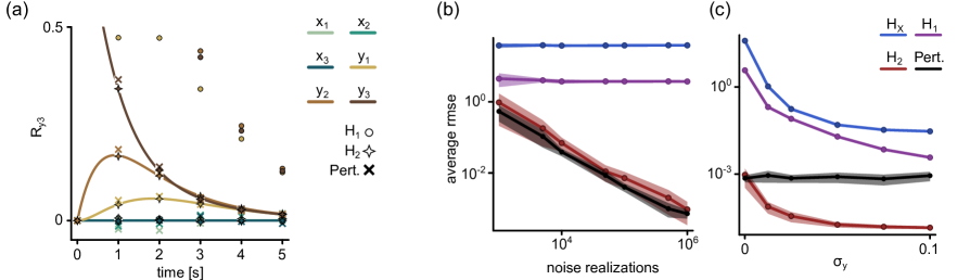
Figure 1: (a), Various estimations of the response function in relation to the perturbing variable $y_{3}$ for a six-dimensional example system as described in (12). The solid line represents the ground truth, while the individual points denote the definitions of perturbation and the fluctuation correlation formula presented in (9), specifically for the first-order $\mathrm{H}_{1}$ and second-order $\mathrm{H}_{2}$ Hermite polynomial observables. Averages over $10^{6}$ experiment realizations for systems parameters $\sigma_{x}=0.1$, $\sigma_{y}=0.025$. (b-c), The average reconstruction error of response curves across all dimensions and time steps, estimated using root mean square error, for the same system depicted in (a). Curves are estimated by perturbation limit and from (9) using observables $\psi_{k}(\mathbf{x})=x_{k}$, named $\mathrm{H}_{x}$, and Hermite basis $\mathrm{H}_{1}$, $\mathrm{H}_{2}$. This analysis considers respectively (b) varying numbers of process realizations ($\sigma_{y}=0.0$) and (c) different levels of noise $\sigma_{y}$ ($10^{6}$ experiments). The shaded ribbon area illustrates the standard deviation resulting from $10$ complete analysis repetitions. The time resolution is set at $\mathrm{dt}=0.01$, perturbation amplitude $\epsilon=0.01$, with stochastic Heun method for integration.

Linear response in non-linear systems –

For system with linear drift and constant diffusion, i.e. a multidimensional Ornstein–Uhlenbeck process [12], the choice $\psi_{k}(\bm{x})=x_{k}$ is sufficient to fully capture the response. In fact in this case the stationary distribution $p_{s}(\bm{x})$ is gaussian and from (10) it follows : $\textbf{R}(t)=\mathbf{C_{xx}}(t)\mathbf{C_{xx}}(0)^{-1}$. Recently in [9] it has been showed that the fluctuation-dissipation formula for linear systems can sometimes yield satisfactory results even in the context of nonlinear dynamics. This is possible only when the stationary distribution is well approximated by a gaussian for the reasons mentioned above. On the other hand our result (9) is the natural generalization that applies for more broad cases paying the cost of extending “virtually” the dimensionality of the systems. In the Koopman literature, the proposed generalization parallels the extension of the Dynamic Mode Decomposition in [16]. As a benchmark, we present an example where a larger list of observables is essential for accurately estimating the correct linear response.

Consider the following nonlinear stochastic differential equation:

$$\begin{cases}d\mathbf{X}=\mathbf{G}_{x}\mathbf{X}dt+\sigma_{x}d\mathbf{W}_{x}\\ d\mathbf{Y}=\mathbf{G}_{y}\mathbf{Y}dt+\mathbf{G}_{yx}\mathbf{X}\odot\mathbf{X}+\sigma_{y}d\mathbf{W}_{y}\end{cases}$$ (12)

where $\odot$ indicates the element-wise product. We have two coupled systems, where the term $\mathbf{G}_{yx}\mathbf{X}\odot\mathbf{X}$ introduces nonlinear interactions between the variables. When considering the case in which $\mathbf{G}_{x}$ is a diagonal matrix, this system can be transformed into a linear one by introducing a new set of observables defined as $\mathbf{Z}=\mathbf{X}\odot\mathbf{X}$, leading to the following evolution

$$\begin{cases}d\mathbf{Z}=2\mathbf{G}_{x}\mathbf{Z}dt+\sigma_{x}^{2}dt+2\sigma_{x}\mathbf{X}\odot d\mathbf{W}_{x}\\ d\mathbf{X}=\mathbf{G}_{x}\mathbf{X}dt+\sigma_{x}d\mathbf{W}_{x}\\ d\mathbf{Y}=\mathbf{G}_{y}\mathbf{Y}dt+\mathbf{G}_{yx}\mathbf{Z}+\sigma_{y}d\mathbf{W}_{y}\end{cases}$$ (13)

If we collect all the degrees of freedom on a vector $\tilde{\mathbf{X}}$, including a constant bias, (13) has the form $d\mathbf{\tilde{X}}=\mathbf{A}\mathbf{\tilde{X}}dt+b(\mathbf{\tilde{X}})d\mathbf{W}$. As we show in the appendix this kind of systems admit an exact finite-size Koopman matrix i.e. $\mathbf{K}(t)=e^{\mathbf{A}t}$ which allows, using (7), to derive analytically the response function of (12).

We analyze the agreement of equation (9) with the exact linear response curves for two sets of observables: i) Hermite functions up to order 1 ($\psi_{k}^{(n)}(\bm{x})=\mathrm{H}_{n}(x_{k})$, $n\in[0,1]$), referred to as $\mathrm{H}_{1}$; ii) Hermite functions up to order 2 ($\psi_{k}^{(n)}(\bm{x})=\mathrm{H}_{n}(x_{k})$, $n\in[0,2]$), referred to as $\mathrm{H}_{2}$ and compare both also to the response function sampled by perturbing the initial conditions, i.e. using the definition (5) and referred to as sampled response. In Fig. 1a an example comparison between these three cases and the exact response function is showed. The average error, see Fig. 1b, associated with $\mathrm{H}_{2}$ scales with the number of realizations in the same way of the sampled response while $\mathrm{H}_{1}$ is order of magnitude worse. This happens because the stationary distribution $p_{s}(\bm{x})$ is asymmetric thus a linear approximation, implicit in $\mathrm{H}_{1}$, will not work. However we note that the increase of the standard deviation $\sigma_{y}$ in (1) mitigates the influence of $\mathrm{X}$ on $\mathrm{Y}$, thereby reducing the asymmetry of its distribution and leading the system to behave more linearly. This effect is clearly shown plotting the average error vs $\sigma_{y}$ (Fig. 1c), with the accuracy of $\mathrm{H}_{1}$ approaches that of the sampled response as $\sigma_{y}$ increases.

From a computational standpoint, equation (9) has been evaluated using a pseudoinverse operation for enhanced efficiency. Specifically, let $\mathbf{V}(t)$ represent the matrix whose columns correspond to the system variables at time $t$, with rows reflecting their values across different realizations of noise, and similarly let $\mathbf{P}(t)$ be the corresponding matrix for the set of functions $\psi$, the virtual response can be estimated as follow

$$\mathbf{\tilde{R}}_{\psi\rightarrow x}(t)=\left[\mathbf{V}(t)\mathbf{P}^{T}(0)\right]\left[\mathbf{P}(0)\mathbf{P}^{T}(0)\right]^{-1}=\mathbf{V}(t)\mathbf{P}^{\dagger}(0)$$

where $\{\cdot\}^{\dagger}$ denotes the pseudoinverse operation.

From response to causality –

It is possible to use the response function as a measure of interventional causality. Following [9], we can measure the strength of the causal dependence of the variable $x_{i}$ on the variable $x_{j}$ as the total response that the former has consequently a perturbation of the latter i.e.:

$$\mathrm{D}_{ij}=\int_{0}^{\infty}\mathrm{R}_{x_{j}\to x_{i}}(t)dt$$ (14)

then using our result (9) we have:

$$\mathbf{D}\approx\left[\int_{0}^{\infty}\mathbf{C_{x\psi}}(t)dt\right]\mathbf{C_{\psi\psi}}(0)^{-1}\braket{\nabla\bm{\psi}}$$ (15)

Thus relating correlation and causality. As expected, the better is the estimation of the response function the better the estimation of the causal link between variables will be. In fact in Fig. 2 we show that the average error on $\mathrm{D}_{ij}$ for the system (1) is substantially higher when we use the basis $\mathrm{H}_{1}$ with respect to $\mathrm{H}_{2}$. It is also noteworthy that by selecting the eigenfunctions $\phi$ of $\mathcal{L}$ as the basis, we derive:

$$\mathrm{D}_{ij}\approx-\sum_{k}\alpha_{ik}\frac{\braket{\partial_{j}\phi_{k}}}{\lambda_{k}}$$

where $\lambda_{k}$ denotes the eigenvalues of $\mathcal{L}$. In essence, this indicates that the causal relationship $\mathrm{D}_{ij}$, can be interpreted as a summation of contributions from $x_{j}$ across the all eigenmodes. These are quantified as $\braket{\partial_{j}\phi_{k}(\bm{k})}$ and are weighted by the significance of each eigenmode, i.e. the associated timescale $1/\lambda_{k}$.

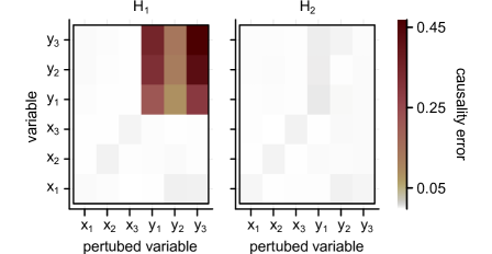
Figure 2: Absolute difference between the exact causality matrix $\mathbf{D}$, normalized by the maximum value, and the estimates obtained using $\mathrm{H}_{1}$ (left) and $\mathrm{H}_{2}$ (right). Values estimated over $10^{6}$ experiment realizations for systems parameters $\sigma_{x}=0.1$, $\sigma_{y}=0.025$, $\mathrm{dt}=0.01$.

Conclusions and future directions –

By establishing a link between the response function and the Koopman operator we derived an alternative way to compute the response function for a general class of non-linear stochastic systems. Our result is rooted in spectral approach that, albeit quite old [22, 23], is now facing renewed interest and widespread adoption [21, 24]. Besides all the possible issues that are common to causality inference as a general, such as non-markovianity [25] and non-stationarity, the major limitation of our result is in the proper choice of the library of basis functions. In fact while convergence can be formally guaranteed when the size of the library goes to infinity, in practice the best would be to find the smallest set of function possible to avoid spectral pollution and over-fitting. A small size in the library is also essential in systems of high dimensions to avoid computational cost. While we will leave to a future work the investigation of this important issue we would like to point toward a possible solution offered by the great approximation capabilities of machine learning algorithm and deep-neural network. For example in [26, 27, 28, 21] the authors showed that already a simple architecture like an auto-encoder is capable to find, by minimizing the loss function

$$||\mathrm{E}[\bm{\psi}(\mathbf{X}_{t})|\mathbf{X}_{0}]-\mathbf{K}(t)\bm{\psi}(\mathbf{X}_{0})||_{2}$$

or its variants, a satisfactory low-dimensional representation of the Koopman operator for the chaotic Lorenz dynamical system and other non-linear examples. The advantage of using simple architectures is that, once the weights of the network are known, the matrix $\partial_{x_{i}}\psi_{j}(\bm{x})$ can be computed analytically.

Being able to infer the causal network of a set of measured variables without the need of perturbing the system is certainly powerful. Thus, given the general premises and the data-driven nature of our results we expect that this approach will be a valuable tool and will find several application in multiple domain of science.

Appendix A The Koopman matrix for system (13)

Consider the general system with a linear drift and arbitrary diffusion and natural boundary conditions:

$$dX_{i}=\bm{A}_{ij}X_{j}dt+b_{ij}(\bm{X})dW_{j}$$ (16)

where we used Einstein notation for repeated indices and $dW_{j}$ are independent Wiener noise sources. Defined the diffusion matrix as $\bm{D}=\bm{b}^{T}\bm{b}/2$, the evolution in time of probability density $p(\bm{X},t|\bm{X}_{0})$ is governed by the following Fokker-Planck equation [13]:

$$\partial_{t}p=-A_{ij}\partial_{i}\left(x_{j}p\right)+\partial_{i}\partial j\left(D_{ij}p\right)$$ (17)

by multiplying (17) by $x_{i}$ and taking the average $\braket{}$ it follows from integration by part that moments follows the linear dynamics:

$$\partial_{t}\mathrm{E}[X_{i,t}|\mathbf{X}_{0}]=A_{ij}\mathrm{E}[X_{j,t}|\mathbf{X}_{0}]$$ (18)

A result commonly refereed to as regression theorem [12]. The solution can be written using the exponential matrix:

$$\mathrm{E}[X_{i,t}|\mathbf{X}_{0}]=e^{\bm{A}t}\mathbf{X}_{0}$$

thus following the definition, the Koopman matrix for this set of observable is: $\bm{K}(t)=e^{\bm{A}t}$

Appendix B Response function from Koopman decomposition

Consider a set of $d$ observables $\{\psi_{k}(\bm{x})\}_{k=1}^{d}$ ideally spanning a subspace containing the state of the system at all times and that admits the family of $d\times d$ matrices $\mathbf{K}(t)$ that approximate the action of the Koopman operators $\mathcal{K}^{t}$.

The average observable evolution in this space, with initial condition $\mathbf{X}_{0}$ is described as

$$\mathrm{E}[\bm{\psi}(\mathbf{X}_{t}|\mathbf{X}_{0}]\approx\mathbf{K}(t)\bm{\psi}(\mathbf{X}_{0})$$ (19)

Under the semi-group assumption it would hold the relation $\mathbf{K}(t)=e^{\mathbf{L}t}$ with $\mathbf{L}$ approximating the action of the infinitesimal Koopman generator $\mathcal{L}$. Note that for $d\to\infty$ convergence is guaranteed and $\mathbf{L}$ becomes iso-spectral to $\mathcal{L}$. In the particular case in which the observables $\psi_{k}$ are the linear evolving eigenfunctions $\phi_{k}$, $\mathbf{K}$ would be the diagonal matrix of the associated eigenvalues $\lambda_{k}$.

Given the coordinates of the state of the system in this space $\bm{x}=\bm{\alpha}\bm{\psi}$, the expected value of the associated stochastic process up to time t is the following

$$\mathrm{E}[\mathrm{X}_{i,t}|\mathbf{X}_{0}]=\sum_{n=1}^{d}\sum_{m=1}^{d}\alpha_{in}\mathrm{K}_{nm}(t)\psi_{m}(\mathbf{X}_{0})$$ (20)

The effect on the physical variable $x_{j}$ of perturbing the function (virtual variable) $\psi_{i}[\mathbf{X}_{0}]\rightarrow\psi_{i}[\mathbf{X}_{0}]+\epsilon_{\psi}$ is then described as

$$\mathrm{E}_{p}[\mathrm{X}_{j,t}|\mathbf{X}_{0}]=\,\mathrm{E}[\mathrm{X}_{j,t}|\mathbf{X}_{0}]+\tilde{\mathrm{R}}_{\psi_{i}\rightarrow x_{j}}(t)\,\epsilon_{\psi}$$

where we introduce $\tilde{\mathrm{R}}_{\psi_{i}\rightarrow x_{j}}(t)$ as the virtual Response function defined by

$$\tilde{\mathrm{R}}_{\psi_{i}\rightarrow x_{j}}(t)=\lim_{\epsilon_{\psi}\to 0}\frac{\langle\mathrm{X}_{j}(t)\rangle_{p}-\langle\mathrm{X}_{j}(t)\rangle}{\epsilon_{\psi}}=[\bm{\alpha}\mathbf{K}(t)]_{ji}$$

where the brackets include the average with respect to the distribution of the initial conditions. Note that for $\psi_{k}$ eigenfunctions and semi-group condition, it holds $\tilde{\mathrm{R}}_{\psi_{i}\rightarrow x_{j}}(t)=\alpha_{ji}e^{\lambda_{i}t}$.

Let’s now look at physical perturbations. Let’s consider the perturbation $\mathrm{X}_{i,0}\rightarrow\mathrm{X}_{i,0}+\epsilon$. Expanding $\psi_{k}[\mathbf{X}_{t}]$ around the unperturbed system we find

$$\mathrm{E}_{p}[\mathrm{X}_{j,t}|\,\mathbf{X}_{0}]=\mathrm{E}[\mathrm{X}_{j,t}|\,\mathbf{X}_{0}]+\epsilon\sum_{m=1}^{d}\left.\frac{\partial\psi_{m}(\mathbf{x})]}{\partial x_{i}}\right|_{\mathbf{X}_{0}}[\bm{\alpha}\mathbf{K}(t)]_{jm}$$

$$=\mathrm{E}[\mathrm{X}_{j,t}|\,\mathbf{X}_{0}]+\epsilon\sum_{m=1}^{d}\left.\frac{\partial\psi_{m}(\mathbf{x})]}{\partial x_{i}}\right|_{\mathbf{X}_{0}}\tilde{\mathrm{R}}_{\psi_{m}\rightarrow x_{j}}(t)$$

Averaging over the initial condition distribution, by the linear response definition we find a relation that links the physical to the virtual response function

$$\text{R}_{x_{i}\rightarrow x_{j}}(t)=\sum_{m=1}^{d}\left\langle\left.\frac{\partial\psi_{m}(\mathbf{x})}{\partial x_{i}}\right|_{\mathbf{X}_{0}}\right\rangle\tilde{\mathrm{R}}_{\psi_{m}\rightarrow x_{j}}(t)$$ (21)

References

- Wiener [1956] N. Wiener, The theory of prediction, Modern mathematics for engineers (1956).
- Granger [1969] C. W. Granger, Investigating causal relations by econometric models and cross-spectral methods, Econometrica: journal of the Econometric Society , 424 (1969).
- Kantz and Schreiber [2003] H. Kantz and T. Schreiber, Nonlinear time series analysis (Cambridge university press, 2003).
- Runge et al. [2023] J. Runge, A. Gerhardus, G. Varando, V. Eyring, and G. Camps-Valls, Causal inference for time series, Nature Reviews Earth & Environment 4, 487 (2023).
- Seth et al. [2015] A. K. Seth, A. B. Barrett, and L. Barnett, Granger causality analysis in neuroscience and neuroimaging, Journal of Neuroscience 35, 3293 (2015).
- Vinci and Benzi [2018] G. V. Vinci and R. Benzi, Economic complexity: Correlations between gross domestic product and fitness, Entropy 20, 766 (2018).
- Javarone et al. [2023] M. A. Javarone, G. Di Antonio, G. V. Vinci, R. Cristodaro, C. J. Tessone, and L. Pietronero, Disorder unleashes panic in bitcoin dynamics, Journal of Physics: Complexity 4, 045002 (2023).
- Marconi et al. [2008] U. M. B. Marconi, A. Puglisi, L. Rondoni, and A. Vulpiani, Fluctuation–dissipation: response theory in statistical physics, Physics reports 461, 111 (2008).
- Baldovin et al. [2020] M. Baldovin, F. Cecconi, and A. Vulpiani, Understanding causation via correlations and linear response theory, Physical Review Research 2, 043436 (2020).
- Rowley et al. [2009] C. W. Rowley, I. Mezić, S. Bagheri, P. Schlatter, and D. S. Henningson, Spectral analysis of nonlinear flows, Journal of fluid mechanics 641, 115 (2009).
- Klus et al. [2020] S. Klus, F. Nüske, S. Peitz, J.-H. Niemann, C. Clementi, and C. Schütte, Data-driven approximation of the koopman generator: Model reduction, system identification, and control, Physica D: Nonlinear Phenomena 406, 132416 (2020).
- Gardiner [2009] C. Gardiner, Stochastic methods, Vol. 4 (Springer Berlin Heidelberg, 2009).
- Risken [1996] H. Risken, The fokker-planck equation (1996).
- Vinci and Mattia [2024] G. V. Vinci and M. Mattia, Escape time in bistable neuronal populations driven by colored synaptic noise, arXiv preprint arXiv:2404.05391 (2024).
- Shizgal [2015] B. Shizgal, Spectral methods in chemistry and physics, Scientific Computation. Springer (2015).
- Williams et al. [2015] M. O. Williams, I. G. Kevrekidis, and C. W. Rowley, A data–driven approximation of the koopman operator: Extending dynamic mode decomposition, Journal of Nonlinear Science 25, 1307 (2015).
- Colbrook et al. [2023] M. J. Colbrook, L. J. Ayton, and M. Szőke, Residual dynamic mode decomposition: robust and verified koopmanism, Journal of Fluid Mechanics 955, A21 (2023).
- Colbrook et al. [2019] M. J. Colbrook, B. Roman, and A. C. Hansen, How to compute spectra with error control, Physical Review Letters 122, 250201 (2019).
- Täuber [2014] U. C. Täuber, Critical dynamics: a field theory approach to equilibrium and non-equilibrium scaling behavior (Cambridge University Press, 2014).
- Note [1] .
- Brunton et al. [2022] S. L. Brunton, M. Budišić, E. Kaiser, and J. N. Kutz, Modern koopman theory for dynamical systems, SIAM Review 64, 229 (2022).
- Koopman [1931] B. O. Koopman, Hamiltonian systems and transformation in hilbert space, Proceedings of the National Academy of Sciences 17, 315 (1931).
- Neumann [1932] J. v. Neumann, Zur operatorenmethode in der klassischen mechanik, Annals of Mathematics 33, 587 (1932).
- Budišić et al. [2012] M. Budišić, R. Mohr, and I. Mezić, Applied koopmanism, Chaos: An Interdisciplinary Journal of Nonlinear Science 22 (2012).
- Capone et al. [2018] C. Capone, G. Gigante, and P. Del Giudice, Spontaneous activity emerging from an inferred network model captures complex spatio-temporal dynamics of spike data, Scientific reports 8, 17056 (2018).
- Lusch et al. [2018] B. Lusch, J. N. Kutz, and S. L. Brunton, Deep learning for universal linear embeddings of nonlinear dynamics, Nature communications 9, 4950 (2018).
- Alford-Lago et al. [2022] D. J. Alford-Lago, C. W. Curtis, A. T. Ihler, and O. Issan, Deep learning enhanced dynamic mode decomposition, Chaos: An Interdisciplinary Journal of Nonlinear Science 32 (2022).
- Otto and Rowley [2019] S. E. Otto and C. W. Rowley, Linearly recurrent autoencoder networks for learning dynamics, SIAM Journal on Applied Dynamical Systems 18, 558 (2019).