Goal-Oriented Communications for Real-time Inference with Two-Way Delay

Abstract

We design a goal-oriented communication strategy for remote inference, where an intelligent model (e.g., a pre-trained neural network) at the receiver side predicts the real-time value of a target signal based on data packets transmitted from a remote location. The inference error depends on both the Age of Information (AoI) and the length of the data packets. Previous formulations of this problem either assumed IID transmission delays with immediate feedback or focused only on monotonic relations where inference performance degrades as the input data ages. In contrast, we consider a possibly non-monotonic relationship between the inference error and AoI. We show how to minimize the expected time-average inference error under two-way delay, where the delay process can have memory. Simulation results highlight the significant benefits of adopting such a goal-oriented communication strategy for remote inference, especially under highly variable delay scenarios.

I Introduction

Intelligent models, e.g. neural networks, have become powerful tools for solving complex computational problems, thanks to advancements in artificial intelligence. These models have not only increased the popularity of today’s most up-to-date technologies but have also played a key role in enabling their current potential. Digital twins, industrial robots, and self-driving cars are prominent examples of such technologies.

An important application of digital twins over long-distance network connections is the monitoring of spacecraft. Consider training a digital twin on Earth based on data coming from rovers on Mars or calibrating the virtual replica of the spacecraft/satellite using live telemetry data [2, 3]. Digital twins have been used in spacecraft design and operations, ranging from assisting ground control in saving the Apollo 13 astronauts to testing thermal protection on the Space Shuttle.

In recent years, digital twins have also gained importance in the monitoring of processes in industrial environments, especially in hazardous or hard-to-reach environments or when it is impractical to be on site for monitoring. One example is the digital twin implementation for the METU high voltage testing laboratory. The digital twin can be monitored over the Internet, and device settings in the physical experiment configuration on site can be remotely changed on demand directly on the twin.

Such systems, involving real-time monitoring, training, etc., often require computation that relies on data sent from remote locations to maintain good performance. Motivated by this, we focus on goal-oriented communication design for the remote inference problem [4, 5]. Goal-oriented communication has been recently introduced to address the scalability problem in next-generation communication networks [6]. This concept emphasizes that networks should focus on the effective accomplishment of the task at the destination rather than merely addressing the transmission problem [7], which aims to reliably transmit data produced by a source. Solving the effective communication problem with efficient use of network resources requires combining the data generation and transmission processes, ensuring that data samples most significant to the computation at the destination are delivered in a timely manner [8]. This implies that the communication link should select which samples to transmit based on the state of the network (e.g., the delay state). Recent efforts in the communication and control communities highlight the value of this approach in reducing communication requirements while maintaining application performance [9, 10, 11, 12, 13, 14].

Since we cannot expect the link layer to operate jointly with the application layer for all possible applications, a surrogate metric that the link layer can utilize when deciding which samples to select and transmit is useful. The Age of Information (AoI) at time $t$, denoted by $\Delta(t)$, is defined in [15] as $\Delta(t)=t-U_{t}$, where $U_{t}$ is the generation time of the most recently delivered data packet. We utilize the AoI as an intermediate metric that can be monitored by the link layer, independent of the specific application. A mapping of application performance in relation to the AoI is all that is required for the link layer to function in a goal-oriented manner. This work builds upon the findings presented in the series of papers [4, 16, 5, 17, 1], which first demonstrated the effectiveness of the AoI metric as a surrogate for enhancing communication in the remote tracking or inference of a process.

In this paper, we study a remote inference problem, where an intelligent model infers the real-time value of a target signal based on data transmitted from a remote location. We assume that the transmitter regularly samples a source and forms data packets containing a number of data samples, which we refer to as the packet length, before each transmission. The intelligent model on the receiver side performs inference using these data packets. The inference error is a function of the AoI and the length of the data packet used by the intelligent model. Recent studies [4, 5] have shown that, in various remote inference problems, the inference error (4) does not always increase monotonically with AoI. This contradicts the conventional assumption that a packet with AoI $=0$ necessarily yields better performance than one with AoI $>0$. Therefore, rather than the generate-at-will model [18, 19], we adopt the “selection-from-buffer” model proposed in [4, 5], which enables the scheduler to choose either fresh or stale data samples from the buffer. Moreover, the inference error decreases monotonically as the packet length increases [17]. This improvement comes at the cost of higher resource usage and increased delay. In our communication design, we explore both the possibly non-monotonic relationship between inference error and AoI, as well as the interplay between packet length and transmission delay.

Due to the need for extreme connectivity, next-generation communication networks are expected to involve numerous connections, leading to the existence of multiple routes between any nodes in the network. The relays in such networks may enforce specific routes for certain data flows, which can dynamically change over time to meet the varying demands of multiple flows. For instance, consider a network involving both terrestrial and non-terrestrial connections. A flow can be fully serviced by non-terrestrial connections, terrestrial connections, or a combination of both, depending on conditions such as the priority of the flow, network congestion, or the availability of satellites. Another example is busy industrial environments, where communication routes may be intermittently unavailable due to shadowing from moving objects, causing flows to be rerouted over time. Consequently, goal-oriented communication design for remote inference must be adaptable to delay conditions significantly varying with memory.

To that end, the technical contributions of this paper are:

• Extending the system models in [5, 17], we formulate and solve a learning and communication co-design problem for remote inference under two-way delay that varies significantly with memory. We consider both time-invariant and time-variable packet length selection scenarios to address the varying computational capabilities of practical systems. The derived optimal scheduling policies minimize the time-average inference error for a given, possibly non-monotonic, inference error function corresponding to a particular remote inference system, thereby making the communication goal-oriented.

• We model the learning and communication co-design problem under time-invariant packet length selection as an infinite-horizon average-cost semi-Markov decision process (SMDP). Such problems are often solved using dynamic programming [20, 21] and typically do not have closed-form solutions. However, we derive a closed-form solution for this scenario, presented in Theorem 1.

• We also model the learning and communication co-design problem under time-variable packet length selection as an infinite-horizon average-cost SMDP. We then formulate a Bellman optimality equation and derive a structural result regarding the optimal solution. Motivated by this result, we present a simplified version of the Bellman optimality equation in Theorem 2. Solving the simplified Bellman equation using dynamic programming has significantly lower time complexity compared to solving the original Bellman optimality equation.

• We conduct two experiments to evaluate the performance of the derived optimal scheduling policies: (i) remote inference of autoregressive (AR) processes, which provides a model-based evaluation; and (ii) cart-pole state prediction, which offers a trace-driven evaluation. Simulation results indicate the substantial benefits of adopting a goal-oriented communication strategy for remote inference.

I-A Related Work

The concept of Age of Information (AoI) has attracted significant research interest; see, e.g., [22, 15, 19, 18, 23, 24, 25, 26, 27, 28, 29, 30, 31, 17, 32, 5, 4, 33, 34] and a recent survey [35]. Initially, research efforts were centered on analyzing and optimizing the average AoI and peak AoI in communication networks [15, 19, 18, 23]. Recent research endeavors have revealed that the performance of real-time applications can be modeled as non-linear functions of AoI, leading to the study of optimizing these non-linear functions in control system scenarios [27, 36], remote estimation [16, 25, 30], and remote inference [22, 4, 17, 5]. While a number of studies have analyzed AoI in queuing models, closest to the spirit of this paper is the control of AoI via replacement of exogenous data arrivals with the generation of data ”at will” [37, 19, 38, 39, 24, 26, 27, 28]. A generalization of this approach is to incorporate jointly optimal sampling and scheduling policies to control not only AoI but a more sophisticated end-to-end distortion criterion by using AoI as an auxiliary parameter [16, 25, 33, 17, 4, 5]. While strikingly more demanding of analysis, these formulations take us closer to goal-oriented communication design.

Almost all previous studies on the “generate-at-will” model adopted an assumption that the penalty of information aging is a non-decreasing function of the AoI [16, 25, 19, 38, 39, 24, 26, 27, 28, 34, 33]. However, it was shown in [22, 4, 17, 32, 5] that the monotonicity of information aging depends heavily on the divergence of the time-series data from being a Markov chain. If the input and target data sequences in a system can be closely approximated as a Markov chain, then the penalty increases as the AoI grows; otherwise, if the data sequence significantly deviates from a Markovian structure, the monotonicity assumption does not hold. Following the approach in [22, 4, 17, 32, 5], this paper models the inference error as a possibly non-monotonic function of AoI.

The works most closely related to this paper are [5, 17], which developed scheduling policies for remote inference, considering a possibly non-monotonic dependency between AoI and practical performance. While [5] developed scheduling policies for fixed packet length, the paper [17] jointly optimized packet length and scheduling strategies. Both the paper [5, 17] considered random IID delay for packet transmissions from the transmitter to the receiver and assumed delay-free feedback from the receiver to the transmitter. In practical systems, a non-zero feedback delay exists [40, 41], which affects the performance of the remote inference algorithm. Moreover, due to the envisioned structure of next-generation communication networks, which contain multiple routes between any pair of nodes, the IID delay may not be a good model. This necessitates a model that captures the memory in the delay process, as in [19]. Extending the problem formulations in [5, 17], this paper designs a goal-oriented communication strategy that minimizes the average inference error for remote inference under two-way delay significantly varying with memory.

II System Model

We consider a remote inference system, which comprises a data source, a transmitter, and a receiver, as illustrated in Fig. 1. On the transmitter side, the source signal $V_{t}$ is regularly sampled from the data source, and the samples are stored in a buffer containing the most recent $B$ samples. The scheduler determines when to transmit and which samples in the buffer to transmit. On the receiver side, a predictor, e.g., a pre-trained neural network, infers the real-time value of a target signal $Y_{t}$ based on the most recently received samples. Such remote inference systems are crucial for many real-time applications, including sensor networks, airplane/vehicular control, robotics networks, and Cyber-Physical Systems (CPS), where timely and accurate remote monitoring and control are essential for maintaining system stability and performance.

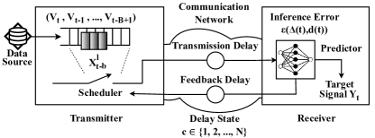
Figure 1: A remote inference system, where the packet $X_{t-b}^{l}$ represents the group of samples $\big{(}V_{t-b},V_{t-b-1},\ldots,V_{t-b-l+1}\big{)}$.

We assume that the system is time-slotted, and it starts operation at time slot $t=0$. We adopt the selection-from-buffer model proposed in [5], where, at each time slot $t$, a new sample of the source signal $V_{t}\in\mathcal{V}$ is added to the buffer while the oldest sample is discarded. The buffer, with size $B$, is assumed to be initially full, storing the samples $\big{(}V_{0},V_{-1},\ldots,V_{-B+1}\big{)}$. Thus, at any time slot $t$, the buffer contains the most recent $B$ samples, $\big{(}V_{t},V_{t-1},\ldots,V_{t-B+1}\big{)}$. Before the $i$-th transmission, the scheduler selects a group of consecutive samples from the buffer and forms the packet $X_{t-b_{i}}^{l_{i}}=\big{(}V_{t-b_{i}},V_{t-b_{i}-1},\ldots,V_{t-b_{i}-l_{i}+1}\big{)}\in\mathcal{V}^{l}$. Here, $l_{i}\in\{1,\ldots,B\}$ and $b_{i}\in\{0,\ldots,B-l_{i}\}$ represents the packet length and buffer position of the $i$-th packet $X_{t-b_{i}}^{l_{i}}$, respectively. Fig. 2 indicates a sample evolution for two consecutive transmission periods. The packet $X_{t-b_{i}}^{l_{i}}$ is submitted at time slot $S_{i}$ and delivered to the receiver at time slot $D_{i}$. Upon delivery, the receiver sends an acknowledgment (ACK) back to the transmitter, which is received at time slot $A_{i}$. We assume that the transmitter always waits for feedback before submitting a new packet. In other words, the transmitter remains silent during the time slots between $S_{i}$ and $A_{i}$ for all $i$.

II-A Communication Network Model

The remote inference system operates on top of a communication network with multiple routes $\{1,2,\ldots,N\}$ connecting the transmitter and the receiver. Each packet submitted into the network is directed to a route based on the network status regarding availability and congestion. If a packet is transmitted through a specific route, its corresponding feedback is also transmitted through that same route. Each route has distinct transmission and feedback delay distributions, and the transmission delay also varies with the packet length. The delay is at least one time slot for each packet or ACK transmission.

Let the $i$-th epoch consist of the time slots in the interval $[A_{i-1},A_{i})$. Define $C_{i}$ as the delay state in the $i$-th epoch, with $c_{i}\in\{1,2,\ldots,N\}$ denoting its realization. The delay state $C_{i}$ represents the network route used in the $i$-th epoch and specifies the transmission and feedback delay distributions. We assume that $C_{i}$ evolves according to a finite-state ergodic Markov chain with transition probabilities $p_{ij}$, where $i,j\in\{1,2,\ldots,N\}$, and $p_{ij}$ represents the probability of transitioning from state $i$ to state $j$. The Markov chain makes a single transition at time slot $A_{i}$ and none otherwise. Let $T_{i}(l_{i})=D_{i}-S_{i}$ and $F_{i}=A_{i}-D_{i}$ represent the transmission and feedback delays incurred in the $i$-th epoch, respectively.

The receiver detects the delay state $c_{i}$ at each delivery time $D_{i}$ and embeds this information into the ACK message. The ACK notifies the scheduler that the previous packet transmission is complete and that the next packet can be submitted to the network. The network is reliable, meaning no packet or message is lost during transmission.

II-B Inference Error

The Age of Information (AoI) on the receiver side, $\Delta(t)$, is the time difference between the current time $t$ and the generation time $t-\Delta(t)$ of the freshest sample $V_{t-\Delta(t)}$ in the most recently delivered packet $X_{t-\Delta(t)}^{l}$. The AoI at time slot $t$ is determined by

$$\Delta(t)=t-S_{i}+b_{i},\text{ if }D_{i}\leq t<D_{i+1}.$$ (1)

Figure 2: A sample evolution for two consecutive transmission periods.

Let $d(t)$ represent the length of the most recently delivered packet by time slot $t$, which can be written as follows:

$$d(t)=l_{i},\text{ if }D_{i}\leq t<D_{i+1}.$$ (2)

We focus on a class of widely used supervised learning algorithms known as Empirical Risk Minimization [42]. We assume that, for each packet length $l\in\{1,2,\ldots,B\}$, the receiver contains a trained neural network $\phi^{*}_{l}\big{(}\cdot\big{)}$ that takes the AoI $\Delta(t)\in\mathbb{Z}^{+}$ and the packet $X_{t-\Delta(t)}^{l}\in\mathcal{V}^{l}$ as inputs and produces an output $a\in\mathcal{A}$ to infer the real-time value of the target signal $Y_{t}\in\mathcal{Y}$. The performance is evaluated through a loss function $L\big{(}\cdot\big{)}:\mathcal{Y}\times\mathcal{A}\mapsto\mathbb{R}$. The incurred loss is $L(y,a)$ when the output $a$ is taken to predict $Y_{t}=y$. Given the AoI $\delta$ and packet length $l$, the training problem to obtain the neural network $\phi^{*}_{l}\big{(}\cdot,\cdot\big{)}$ is formulated as:

$$\min_{\phi\big{(}\cdot,\cdot\big{)}\in\Lambda}\mathbb{E}_{Y,X^{l}\sim P_{\tilde{Y}_{0},\tilde{X}_{-\delta}^{l}}}\big{[}L\big{(}Y,\phi\big{(}\delta,X^{l}\big{)}\big{)}\big{]},$$ (3)

where $\Lambda$ is the set of all mappings that the neural network can generate, and $P_{\tilde{Y}_{0},\tilde{X}_{-\delta}^{l}}$ represents the empirical distribution of the target signal $\tilde{Y}_{0}$ and the packet $\tilde{X}_{-\delta}^{l}$. The AoI $\delta$ is the time difference between the generation of $\tilde{Y}_{0}$ and $\tilde{X}_{-\delta}$.

These trained predictors are used to estimate the real-time value of the target signal $Y_{t}$ on the receiver side. We assume that the process $\{\big{(}Y_{t},V_{t}\big{)},t=0,1,\ldots\}$ is stationary, and that the processes $\{\big{(}Y_{t},V_{t}\big{)},t=0,1,\ldots\}$ and $\{\big{(}\Delta(t),d(t)\big{)},t=0,1,\ldots\}$ are independent. The average inference error at time slot $t$, given $\Delta(t)=\delta$ and $d(t)=l$, is expressed as:

$$\varepsilon\big{(}\delta,l\big{)}=\mathbb{E}_{Y,X^{l}\sim P_{Y_{t},X_{t-\delta}^{l}}}\big{[}L\big{(}Y,\phi^{*}_{l}\big{(}\delta,X^{l}\big{)}\big{)}\big{]},$$ (4)

where $P_{Y_{t},X_{t-\delta}^{l}}$ represents the joint distribution of the target signal $Y_{t}$ and the packet $X_{t-\delta}^{l}$.

We are interested in loss functions $L\big{(}\cdot\big{)}$ for which the inference error (4) is bounded. Apart from this restriction, the loss function $L\big{(}\cdot\big{)}$ can be chosen based on the goal of the remote inference system. For example, a quadratic loss function $L_{2}\big{(}y,\hat{y}\big{)}=\lVert y-\hat{y}\rVert_{2}^{2}$ is used in neural network-based minimum mean-squared estimation, where the action $a=\hat{y}$ is an estimate of the target signal $Y_{t}=y$ and $\lVert y\rVert_{2}$ is the Euclidean norm. In softmax regression (i.e., neural network-based maximum likelihood classification), the action $a=\mathcal{Q}_{Y}$ is a distribution of $Y_{t}$, and the loss function $L_{\log}\big{(}y,\mathcal{Q}_{Y}\big{)}=-\log\mathcal{Q}_{Y}(y)$ is the negative log-likelihood function of the value $Y_{t}=y$.

In the subsequent sections, we solve a learning and communication co-design problem that aims to optimize the performance of a remote inference system. From equation (4), we know that the inference error is a function of both the AoI and packet length. For a given AoI $\delta$, the inference error is a non-increasing function of packet length [17]. However, for a given packet length $l$, the inference error does not always increase monotonically with the AoI [4, 5]. This observation contradicts the conventional assumption that fresher packets yield smaller inference errors. Theoretical and experimental explanations of this counter-intuitive observation was provided in [4, 5]. Therefore, we do not adopt the generate-at-will model [18, 19] in this paper.

II-C Structure of a Scheduling Policy

Upon the ACK reception time $A_{i}$, the scheduler determines a waiting time $\tau_{i+1}$ to specify the next submission time slot $S_{i+1}=A_{i}+\tau_{i+1}$. Then, a data packet $X_{S_{i+1}-b_{i+1}}^{l_{i+1}}$ is formed by selecting the packet length $l_{i+1}$ and buffer position $b_{i+1}$. A scheduling policy $\pi\in\Pi$ is defined as a tuple $\pi=\big{(}f,\ell,g\big{)}$, where $f=\big{(}b_{2},b_{3},\ldots\big{)}$ is the buffer position sequence, $\ell=\big{(}l_{2},l_{3},\ldots\big{)}$ is the packet length sequence, $g=\big{(}\tau_{2},\tau_{3},\ldots\big{)}$ is the waiting time sequence, and $\Pi$ denotes the set of all causal policies $\pi$. We assume that the scheduling policy does not employ the knowledge of the observed process $\{\big{(}Y_{t},V_{t}\big{)},t=0,1,\ldots\}$. This assumption implies that the processes $\{\big{(}Y_{t},V_{t}\big{)},t=0,1,\ldots\}$ and $\{\big{(}\Delta(t),d(t)\big{)},t=0,1,\ldots\}$ are independent. The initial conditions of the system are assumed to be $S_{1}=0$, $l_{1}=1$, $b_{1}=0$, $c_{1}\in\{1,2,\ldots,N\}$, and $\Delta(0)$ is a finite constant.

III Learning and Communications Co-design: Time-invariant Packet Length Selection

While designing goal-oriented communication protocols for remote inference, selecting a constant packet length is a simple and often effective choice. If packet lengths vary dynamically from one packet to the next, the receiver needs to reconfigure the estimator over time to accommodate the changing input dimensions, which adds complexity. In this section, we consider systems where this complexity is avoided by choosing a time-invariant packet length sequence. Systems that can vary the packet length over time are discussed in Section IV.

III-A Co-design Problem Formulation

Let $\Pi_{l}$ represent the set of all causal scheduling policies $\pi=(f,\ell,g)$ with a time-invariant packet length sequence ${\ell=\{l,l,\ldots\}}$ for $l\in\{1,2,\ldots,B\}$:

$$\Pi_{l}=\{\pi\in\Pi:l=l_{2}=l_{3}=\ldots\}.$$ (5)

The learning and communications co-design problem with time-invariant packet length selection can be formulated as a two-layer nested optimization problem:

$$\varepsilon_{l,\text{opt}}=\inf_{\pi\in\Pi_{l}}\limsup_{T\to\infty}\frac{1}{T}\mathbb{E}_{\pi}\Bigg{[}\sum_{t=0}^{T-1}\varepsilon\big{(}\Delta(t),l\big{)}\Bigg{]},$$ (6)

$$\varepsilon_{\text{opt}}^{\text{inv.}}=\min_{l\in\{1,2,\ldots,B\}}\varepsilon_{l,\text{opt}},$$ (7)

where $\varepsilon_{l,\text{opt}}$ is the optimum value of the inner optimization problem (6) for a given packet length $l$, and $\varepsilon_{\text{opt}}^{\text{inv.}}$ is the optimum value of the two-layer nested optimization problem (6)-(7) with the optimal time-invariant packet length.

The inner optimization problem (6) can be cast as an infinite-horizon average-cost Semi-Markov Decision Process (SMDP). While dynamic programming algorithms, namely policy iteration and value iteration, are typically employed to solve such problems [20, 21], we are able derive a closed-form solution that achieves significantly lower computational complexity than dynamic programming. Moreover, the outer optimization problem (7) is a straightforward search over the integer values $\{1,2,\ldots,B\}$.

Unlike the formulation in [17], this problem formulation accounts for varying delay conditions between the transmitter and the receiver and does not assume immediate feedback.

III-B Optimal Solution to (6)-(7)

We define each ACK reception time $A_{i}$ as a decision time for the SMDP (6). The system state at time slot $A_{i}$ is represented by a tuple $\big{(}\delta,c_{i}\big{)}$, where $\delta=\Delta(A_{i})$ and $c_{i}$ is the delay state in the $i$-th epoch. The actions are the waiting time $\tau_{i+1}$ and the buffer position $b_{i+1}$. A detailed description of the SMDP can be found in Appendix A. The Bellman optimality equation of this SMDP can be formulated as:

$$h_{1}\big{(}\delta,c_{i}\big{)}=\min_{\begin{subarray}{c}\tau_{i+1}\in\{0,1,\ldots\}\\ b_{i+1}\in\{0,1,\ldots,B-l\}\end{subarray}}$$

$$\mathbb{E}\Bigg{[}\sum_{k=0}^{\tau_{i+1}+T_{i+1}(l)-1}\bigg{(}\varepsilon\big{(}\delta+k,l\big{)}-\varepsilon_{l,\text{opt}}\bigg{)}\Bigg{|}C_{i}=c_{i}\Bigg{]}$$

$$+\mathbb{E}\Bigg{[}\sum_{k=0}^{F_{i+1}-1}\bigg{(}\varepsilon\big{(}b_{i+1}+T_{i+1}(l)+k,l\big{)}-\varepsilon_{l,\text{opt}}\bigg{)}\Bigg{|}C_{i}=c_{i}\Bigg{]}$$

$$+\mathbb{E}\big{[}h_{1}\big{(}b_{i+1}+T_{i+1}(l)+F_{i+1},C_{i+1}\big{)}\big{|}C_{i}=c_{i}\big{]},$$ (8)

where $h_{1}(\delta,c_{i})$ is the relative value function. We need to solve the Bellman optimality equation (III-B) to find an optimal solution to (6). This involves determining the optimal buffer position $b_{i+1}^{*}$ and waiting time $\tau_{i+1}^{*}$ for each state $\big{(}\delta,c_{i}\big{)}$. By exploiting the structural properties of the Bellman optimality equation (III-B), we are able to obtain a closed-form solution to (6), as asserted in the following theorem.

Define the index function

$$\gamma\big{(}\delta,d,l,c\big{)}=\min_{\tau\in\{1,2,\ldots\}}\frac{1}{\tau}\sum_{k=0}^{\tau-1}\mathbb{E}\bigg{[}\varepsilon\big{(}\delta+T_{i+1}(l)+k,d\big{)}\bigg{|}C_{i}=c\bigg{]},$$ (9)

for all $\delta\in\{1,2,\ldots\}$, $d,l\in\{1,2,\cdot,B\}$, and $c\in\{1,2,\ldots,N\}$.

Theorem 1.

There exists an optimal solution $\pi^{*}=\big{(}\big{(}b_{2}^{*},b_{3}^{*},\ldots\big{)},\big{(}l,l,\ldots\big{)},\big{(}\tau_{2}^{*},\tau_{3}^{*},\ldots\big{)}\big{)}\in\Pi_{l}$ to problem (6), where the optimal waiting time $\tau_{i+1}^{*}$ is determined by the index-based threshold rule

$$\tau_{l}\big{(}\delta,c_{i}\big{)}=\min\{k\geq 0:\gamma\big{(}\delta+k,l,l,c_{i}\big{)}\geq\beta\},$$ (10)

the optimal buffer position $b_{i+1}^{*}$ is given by

$$b_{i+1}^{*}=\operatorname*{arg\,min}_{b\in\{0,1,\ldots,B-l\}}$$

$$\mathbb{E}\Bigg{[}\sum_{k=0}^{\mathfrak{D}-1}\bigg{(}\varepsilon\big{(}b+T_{i+1}(l)+k,l\big{)}-\beta\bigg{)}\Bigg{|}C_{i}=c_{i}\Bigg{]},$$ (11)

$\mathfrak{D}=F_{i+1}+\tau_{l}\big{(}b+T_{i+1}(l)+F_{i+1},C_{i+1}\big{)}+T_{i+2}(l)$, and $\gamma\big{(}\cdot\big{)}$ is defined in (9). Furthermore, $\beta$ is the unique root of

$$\mathbb{E}\Bigg{[}\sum_{t=A_{i}(\beta)}^{A_{i+1}(\beta)-1}\varepsilon\big{(}\Delta(t)\big{)}\Bigg{]}-\beta\mathbb{E}\big{[}A_{i+1}(\beta)-A_{i}(\beta)\big{]}=0,$$ (12)

and it is exactly the optimum value $\varepsilon_{l,\text{opt}}$ of problem (6).

Proof Sketch.

We prove Theorem 1 in three steps:

Step 1: We obtain two key results by using the Bellman optimality equation (III-B):

• The optimal waiting time $\tau_{i+1}^{*}$ is determined by the threshold rule $\tau_{l}\big{(}\delta,c_{i}\big{)}$ given by equation (10) for all $i$.

• The delay state $c_{i}$ in the $i$-th epoch is a sufficient statistic for determining the optimal buffer position $b_{i+1}^{*}$ for all $i$.

Step 2: Since the delay state $c_{i}$ in the $i$-th epoch is a sufficient statistic for determining $b_{i+1}^{*}$ for all $i$, we can construct a new SMDP for determining $b_{i+1}^{*}$ using $c_{i}$ as the state. In the new SMDP, we fix the waiting time decisions by using optimal threshold rule $\tau_{l}\big{(}\delta,c_{i}\big{)}$. Moreover, in the new SMDP, the decision time is $D_{i+1}$ instead of $A_{i}$. The Bellman optimality equation of this new SMDP is expressed as:

$$h_{1}^{\prime}\big{(}c_{i}\big{)}=\min_{\begin{subarray}{c}b_{i+1}\in\{0,1,\ldots,B-l\}\end{subarray}}$$

$$\mathbb{E}\Bigg{[}\sum_{k=0}^{\vartheta_{i+1}-1}\bigg{(}\varepsilon\big{(}b_{i+1}+T_{i+1}(l)+k,l\big{)}-\varepsilon_{l,\text{opt}}\bigg{)}\Bigg{|}C_{i}=c_{i}\Bigg{]}$$

$$+\mathbb{E}\bigg{[}h_{1}^{\prime}\big{(}C_{i+1}\big{)}\bigg{|}C_{i}=c_{i}\bigg{]},$$ (13)

where $\vartheta_{i+1}=F_{i+1}+\tau_{l}\big{(}b_{i+1}+T_{i+1}(l)+F_{i+1},C_{i+1}\big{)}+T_{i+2}(l)$, and $h_{1}^{\prime}\big{(}c_{i}\big{)}$ is the relative value function.

The Bellman optimality equation (III-B) is decomposable and can be solved as a per-decision-epoch optimization problem, allowing any $b_{i+1}^{*}$ in the optimal buffer position sequence ${f^{*}=\big{(}b_{2}^{*},b_{3}^{*},\ldots\big{)}}$ to be expressed as shown in (1).

Step 3: We determine that the optimal value $\varepsilon_{l,\text{opt}}$ for the inner optimization problem (6) is the unique root of (12).

The detailed proof is provided in Appendix B. ∎

The optimal scheduling policy for the inner optimization problem (6), outlined in Theorem 1, is well-structured. Each optimal waiting time $\tau_{i+1}^{*}$ is determined by an index-based threshold rule $\tau_{l}\big{(}\delta,c_{i}\big{)}$. The index function $\gamma\big{(}\cdot\big{)}$, provided in (9), can be readily calculated for any state $\big{(}\delta,c_{i}\big{)}$, using the conditional distribution of $T_{i+1}(l)$ given $C_{i}=c_{i}$.

Furthermore, according to equation (1), $b_{i+1}^{*}$ is designed to minimize the relative inference error in the interval between $D_{i+1}$ and $D_{i+2}$, given that the waiting time is determined by the optimal rule in (10). Also, each optimal buffer position $b_{i+1}^{*}$ depends solely on the delay state $c_{i}$ in the $i$-th epoch, and is independent of $\delta=\Delta(A_{i})$. This result can be better understood by deeply analyzing the AoI evolution. At each delivery time slot $D_{i+1}$, the AoI resets to a realization of $b_{i+1}^{*}+T_{i+1}(l)$. Due to these regular resets, the AoI evolution between consecutive delivery slots $D_{i+1}$ and $D_{i+2}$ is independent of the AoI evolution outside this interval. Moreover, $b_{i+1}^{*}$ is a parameter to control the AoI evolution between $D_{i+1}$ and $D_{i+2}$.

Finally, the optimum value $\varepsilon_{l,\text{opt}}$, which is the threshold in the waiting time rule (10) and necessary for solving (1), is the unique root of equation (12). This equation can be efficiently solved using low-complexity algorithms [25, Algorithms 1-3], such as bisection search.

The optimal policy in Theorem 1 has two key distinctions compared to the policy established in [17, Theorem 1] for remote inference under time-invariant packet length selection, IID transmission delays, and immediate feedback. First, although the threshold rule $\tau_{l}\big{(}\delta,c_{i}\big{)}$ in (10) closely resembles the waiting time rule derived in [17, Theorem 1], it is not solely dependent on the AoI but also incorporates the delay state. For the problem formulation (6)-(7), which involves a finite number of delay states with non-zero feedback delay, the existence of such a waiting time rule was not evident and required additional technical efforts for its derivation.

Second, in [17, Theorem 1], the optimal buffer position sequence is time-invariant due to the assumption of IID transmission delays. However, when the delay state changes with memory, achieving optimal performance requires a buffer position sequence that can adapt to variations in delay statistics. Theorem 1 unveils that the optimal buffer position sequence is determined by solving $N$ per-sample optimization problems, each related to a distinct delay state, without requiring pre-computation of the relative value function $h_{1}\big{(}\cdot\big{)}$.

We can solve the inner optimization problem (6) for any given packet length $l$ by using Theorem 1. Then, the outer optimization problem (7) is just a straightforward search over the integer values $\{1,2,\ldots,B\}$, and $\varepsilon_{\text{opt}}^{\text{inv.}}=\varepsilon_{l^{*},\text{opt}}$.

IV Learning and Communications Co-design: Time-Variable Packet Length Selection

In contrast to the previous case, where high computational complexity is avoided, here we aim to achieve optimal performance without any restrictions on the packet length sequence $\ell=\big{(}l_{2},l_{3},\ldots\big{)}$. This unconstrained approach allows us to maximize the system’s potential by dynamically adjusting the packet length $l_{i}$ over time. Therefore, this case represents the most general solution.

IV-A Co-design Problem Formulation

The learning and communications co-design problem with time-variable packet length selection is formulated as:

$$\varepsilon_{\text{opt}}=\inf_{\pi\in\Pi}\limsup_{T\to\infty}\frac{1}{T}\mathbb{E}_{\pi}\Bigg{[}\sum_{t=0}^{T-1}\varepsilon\big{(}\Delta(t),d(t)\big{)}\Bigg{]},$$ (14)

where $\varepsilon_{\text{opt}}$ is the optimum value of problem (14).

Problem (14) is an infinite-horizon average-cost SMDP, which is more challenging to solve compared to problem (6). We formulate a Bellman optimality equation for this SMDP and then simplify it using a structural result regarding the optimal policy. The time complexity for solving the simplified Bellman optimality equation using dynamic programming algorithms is substantially lower than that for solving the original Bellman optimality equation.

IV-B Optimal Solution to (14)

Each ACK reception time $A_{i}$ is a decision time for the SMDP (14). The system state at time slot $A_{i}$ is represented by a tuple $\big{(}\delta,d,c_{i}\big{)}$, where $\delta=\Delta(A_{i})$, $d=d(A_{i})$, and $c_{i}$ is the delay state in the $i$-th epoch. The actions to be taken at each decision time $A_{i}$ are the waiting time $\tau_{i+1}$, the packet length $l_{i+1}$, and the buffer position $b_{i+1}$. A detailed description of the SMDP can be found in Appendix C. The Bellman optimality equation of this SMDP can be expressed as:

$$h_{2}\big{(}\delta,d,c_{i}\big{)}=\min_{\begin{subarray}{c}\tau_{i+1}\in\{0,1,\ldots\}\\ l_{i+1}\in\{1,2,\ldots,B\}\\ b_{i+1}\in\{0,1,\ldots,B-l_{i+1}\}\end{subarray}}$$

$$\mathbb{E}\Bigg{[}\sum_{k=0}^{\tau_{i+1}+T_{i+1}(l_{i+1})-1}\bigg{(}\varepsilon\big{(}\delta+k,d\big{)}-\varepsilon_{\text{opt}}\bigg{)}\Bigg{|}C_{i}=c_{i}\Bigg{]}$$

$$+\mathbb{E}\Bigg{[}\sum_{k=0}^{F_{i+1}-1}\bigg{(}\varepsilon\big{(}b_{i+1}+T_{i+1}(l_{i+1})+k,l_{i+1}\big{)}-\varepsilon_{\text{opt}}\bigg{)}\Bigg{|}C_{i}=c_{i}\Bigg{]}$$

$$+\mathbb{E}\big{[}h_{2}\big{(}b_{i+1}+T_{i+1}(l_{i+1})+F_{i+1},l_{i+1},C_{i+1}\big{)}\big{|}C_{i}=c_{i}\big{]},$$ (15)

where $h_{2}\big{(}\delta,d,c_{i}\big{)}$ is the relative value function.

By solving the Bellman optimality equation (IV-B) using dynamic programming, we can obtain a solution to problem (14). The time complexity of this dynamic programming algorithm is high, as it requires the joint optimization of three variables for each state $\big{(}\delta,d,c_{i}\big{)}$. Theorem 2 provides a threshold rule for determining the waiting time action at each decision time $A_{i}$ and simplifies the Bellman optimality equation. The time complexity for solving the simplified Bellman optimality equation is significantly lower than that for solving (IV-B).

Theorem 2.

There exists an optimal solution $\pi^{*}=\big{(}\big{(}b_{2}^{*},b_{3}^{*},\ldots\big{)},\big{(}l_{2}^{*},l_{3}^{*},\ldots\big{)},\big{(}\tau_{2}^{*},\tau_{3}^{*},\ldots\big{)}\big{)}\in\Pi$ to problem (14). The optimal waiting time $\tau_{i+1}^{*}$ is determined by the index-based threshold rule

$$\tau\big{(}\delta,d,l_{i+1},c_{i}\big{)}=\min\{k\geq 0:\gamma\big{(}\delta+k,d,l_{i+1},c_{i}\big{)}\geq\varepsilon_{\text{opt}}\},$$ (16)

where $\gamma\big{(}\cdot\big{)}$ is defined in (9). Furthermore, the optimal packet length $l_{i+1}^{*}$ and buffer position $b_{i+1}^{*}$ are determined by solving the simplified Bellman optimality equation

$$h_{2}\big{(}\delta,d,c_{i}\big{)}=\min_{l_{i+1}\in\{1,2,\ldots,B\}}\big{\{}$$

$$\mathbb{E}\Bigg{[}\sum_{k=0}^{\tau\big{(}\delta,d,l_{i+1},c_{i}\big{)}+T_{i+1}(l_{i+1})-1}\bigg{(}\varepsilon\big{(}\delta+k,d\big{)}-\varepsilon_{\text{opt}}\bigg{)}\Bigg{|}C_{i}=c_{i}\Bigg{]}$$

$$+\min_{b_{i+1}\in\{0,1,\ldots,B-l_{i+1}\}}\big{\{}$$

$$\mathbb{E}\Bigg{[}\sum_{k=0}^{F_{i+1}-1}\bigg{(}\varepsilon\big{(}b_{i+1}+T_{i+1}(l_{i+1})+k,l_{i+1}\big{)}-\varepsilon_{\text{opt}}\bigg{)}\Bigg{|}C_{i}=c_{i}\Bigg{]}$$

$$+\mathbb{E}\big{[}h_{2}\big{(}b_{i+1}+T_{i+1}(l_{i+1})+F_{i+1},l_{i+1},C_{i+1}\big{)}\big{|}C_{i}=c_{i}\big{]}\big{\}}\big{\}}.$$ (17)

Proof Sketch.

Theorem 2 is proved motivated by the observation that the optimal waiting time $\tau_{i+1}^{*}$ and buffer position $b_{i+1}^{*}$ for any state $\big{(}\delta,d,c_{i}\big{)}$ can be determined by solving separate optimization problems, given the optimal packet length $l_{i+1}^{*}$. Subsequently, the solution to the waiting time problem is derived as an index-based threshold rule, which allows us to simplify the Bellman optimality equation (IV-B) to (2). The detailed proof is provided in Appendix E. ∎

Both Bellman optimality equations (IV-B) and (2) for the SMDP (14) can be solved using policy iteration, value iteration, or linear programming [20, Chapter 11.4.4]. Policy iteration is efficient for solving SMDPs [17, 20]. The time complexity for solving the simplified Bellman equation (2) is significantly lower than that for solving (IV-B). The policy improvement step for (IV-B) has a time complexity of $O(\tau_{\text{bound}}^{2}B^{3})$, while it is $O(\tau_{\text{bound}}^{2}B+\tau_{\text{bound}}B^{3}+\tau_{\text{bound}}B^{2})=O(\max\{\tau_{\text{bound}}^{2}B,\tau_{\text{bound}}B^{3}\})$ for the simplified equation (2). The policy evaluation step is identical for both equations.

V Simulations

To evaluate the performance of the optimal scheduling policies outlined in Theorems 1 and 2, we consider two experiments: (i) remote inference of autoregressive (AR) processes, which provides a model-based evaluation; and (ii) cart-pole state prediction, which provides a trace-driven evaluation.

V-A Model-Based Evaluation

Control systems with memory and delay [43, 44, 45] and wireless channels [46] are often modeled as higher-order autoregressive (AR) linear time-invariant systems. Motivated by this, we consider a remote inference problem for an AR process, where the target evolves according to:

$$Y_{t}=a_{1}Y_{t-1}+a_{2}Y_{t-2}+\ldots+a_{p}Y_{t-p}+W_{t},$$ (18)

where the noise $W_{t}\in\mathbb{R}$ is zero-mean Gaussian with variance $\sigma_{W}^{2}$ and $Y_{t}\in\mathbb{R}$. Let $V_{t}=Y_{t}+N_{t}$ be the noisy observation of the target $Y_{t}$, where $N_{t}\in\mathbb{R}$ is zero-mean Gaussian with variance $\sigma_{N}^{2}$. We set $\sigma_{W}^{2}=0.01$, $\sigma_{N}^{2}=0.001$ and construct an AR($10$) process with coefficients $a_{2}=0.05$ and $a_{10}=0.9$. The remaining coefficients are zero. We consider a quadratic loss function $L_{2}(y,\hat{y})=\lVert y-\hat{y}\rVert_{2}^{2}$. In this experiment, the goal is to infer the target signal $Y_{t}$ by using the data packet $X_{t-\delta}^{l}=(V_{t-\delta},V_{t-\delta-1},\ldots,V_{t-\delta-l+1})$. Since $X_{t-\delta}^{l}$ and $Y_{t}$ are jointly Gaussian, and the loss function is quadratic, the optimal inference error is achieved by a linear MMSE estimator. Fig. 3 shows the average inference error for AoI values $\delta=1,2,\ldots,40$ and packet lengths $l=1,2,4,6,8,10$.

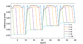
Figure 3: Inference error of the AR process experiment for AoI values $\delta=1,2,\ldots,40$ and packet lengths $l=1,2,4,6,8,10$.

Using this AR process experiment, we illustrate the performance of the optimal policy derived for the scheduling problem (6)-(7) under time-invariant packet length selection. Let the number of delay states $N$ be $2$. The transmission delay $T_{i}(l)$ corresponding to each state is given by

$$T_{i}(l)=\begin{cases}\lceil\sigma l\rceil,&\text{if }c_{i}=1\\ \lceil 5\sigma l\rceil,&\text{if }c_{i}=2\end{cases},$$ (19)

where $\sigma$ is a scaling parameter. The feedback delay $F_{i}$ is $1$ time slot when $c_{i}=1$ and $3$ time slots when $c_{i}=2$. We adjust the delay memory using the parameter $\alpha=p_{12}+p_{21}$, which is equal to the sum of transition probabilities of the Markov chain according to which the delay state evolves. We set $p_{12}=p_{21}$, ensuring that the fraction of epochs with convenient delay conditions is $\frac{1}{2}$ in the steady state for any $\alpha$. The maximum allowed packet length is 10, and the buffer size $B=75$.

Fig. 4 presents the time-average inference error achieved by the following three scheduling policies as the parameter $\sigma$ changes from $0$ to $2$ with $\alpha=\frac{1}{20}$:

• Optimal policy derived for the scheduling problem (6)-(7) under time-invariant packet length selection.

• Policy outlined in Theorem 1 for $l=1$.

• Generate-at-will, zero-wait, $l=1$ policy: $(f,\ell,g)$ such that $f=g=(0,0,\ldots)$ and $\ell=(1,1,\ldots)$.

The result in Fig. 4 highlights that the first policy achieves a time-average inference error up to 6 times smaller compared to the third policy. Although part of this gain can be obtained with the packet length $l=1$ by optimally determining the waiting times and buffer positions as in the second policy, a larger portion of the gain comes from selecting the appropriate packet length, accounting for the interplay between the transmission delay statistics and the packet length $l$.

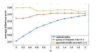
Figure 4: Time-average inference error vs. the scaling parameter $\sigma$ of transmission delay $T_{i}(l)$.

Fig. (5) presents the time-average inference error achieved by the following two scheduling policies as the parameter $\alpha$ varies from $0$ to $2$ with $\sigma=\frac{5}{2}$:

• Policy outlined in Theorem 1 for $l=5$.

• Policy outlined in [17, Theorem 1] for a fixed packet length of $l=5$. During the simulations, this policy assumes that both delay states are equally likely at each epoch, independent of the history, for any $\alpha$.

The result in Fig. (5) emphasizes the importance of considering delay memory when designing scheduling algorithms. It demonstrates that the first policy offers minimal improvement compared to the second policy when $\alpha$ is close to $1$. This is because the delay distribution becomes exactly IID at $\alpha=1$. However, as $\alpha$ deviates from this value, the delay memory increases, and the advantage of the first policy becomes apparent, with a significant performance gain of up to $11.6\%$.

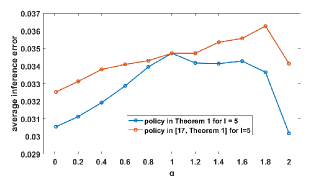
Figure 5: Time-average inference error vs. the sum of transition probabilities $\alpha=p_{12}+p_{21}$.

V-B Trace-Driven Evaluation

We consider the OpenAI CartPole-v1 task [47], where a Deep Q-Network (DQN) reinforcement learning algorithm [48] is used to control the force applied to a cart to prevent the attached pole from falling over. A pre-trained DQN neural network from [5] is employed for this control task. A time-series dataset containing the pole angle $\psi_{t}$ and cart position $Z_{t}$ is obtained from [5]. This dataset was generated by simulating 10,000 episodes of the OpenAI CartPole-v1 environment using the DQN controller. The objective is to predict the pole angle and position $Y_{t}=(\psi_{t},Z_{t})$ at time $t$ based on the feature vector $X_{t-\delta}=\big{(}(\psi_{t-\delta},Z_{t-\delta}),\ldots,(\psi_{t-\delta+l-1},Z_{t-\delta+l-1})\big{)}$, which represents a sequence of past pole angles and cart positions generated $\delta$ time slots ago, with a sequence length of $l$.

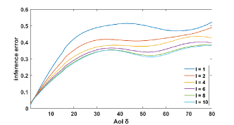
Figure 6: Inference error of the cart-pole experiment for AoI values $\delta=1,2,\ldots,80$ and feature vector lengths $l=1,2,4,6,8,10$.

Ensuring the safe operation of industrial and robotic systems often requires evaluating their state based on observations from remote sources. Consequently, the prediction problem is critical for monitoring the safety of these systems. We focus on a specific scenario where a camera remotely monitors a cart-pole system. The camera captures video frames and transmits them to a receiver. Due to the high dimensionality of the video data, transmitting the sequence of frames requires multiple time slots. Consequently, the most recently delivered sequence of video frames is generated $\delta$ time slots ago. Once received, the frames undergo signal processing to extract relevant information about the cart’s position and the pole’s angle. We assume this signal processing is accurate. Then, a predictor takes the most recent available observations and predicts the current pole angle and cart position $Y_{t}=(\psi_{t},Z_{t})$.

The predictor in this experiment is a Long Short-Term Memory (LSTM) neural network consisting of one input layer, one hidden layer with 64 LSTM cells, and a fully connected output layer. The first 72% of the dataset is used for training, and the remaining data is used for inference. The performance of the trained LSTM predictor is evaluated on the inference dataset. The inference error is shown in Fig. 6 for AoI values $\delta=1,2,\ldots,80$ and feature vector lengths $l=1,2,4,6,8,10$. We observe that the inference error is not a monotonic function of AoI $\delta$ for a given feature vector length $l$. Additionally, the inference error decreases as the feature vector length $l$ increases for a fixed AoI value $\delta$.

Using this cart-pole experiment, we illustrate the performance of the optimal policy outlined in Theorem 2, which is derived for the scheduling problem (14) under time-variable packet length selection. We again consider two delay states, i.e., ${N=2}$. The transmission delay $T_{i}(l)$ is given by

$$T_{i}(l)=\begin{cases}\lceil\sigma l\rceil,&\text{if }c_{i}=1\\ 5+\lceil 5\sigma l\rceil,&\text{if }c_{i}=2\end{cases},$$ (20)

where $\sigma$ is a scaling parameter. The feedback delay $F_{i}$ is identical to that in the AR process experiment. We set the parameter $\alpha=p_{12}+p_{21}=\frac{1}{20}$. The transition probabilities $p_{12}$ and $p_{21}$ are equal, ensuring that the fraction of epochs with convenient delay conditions is $\frac{1}{2}$ in steady state for any $\alpha$.

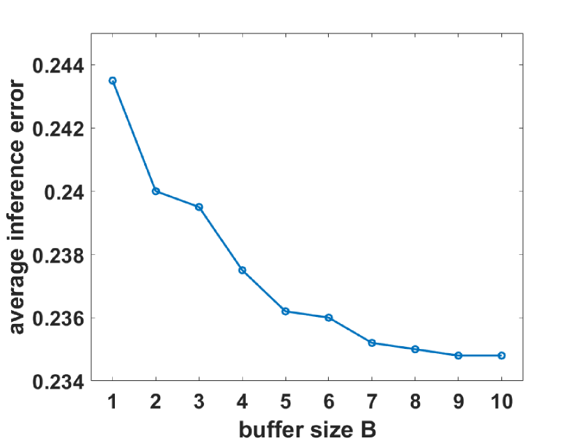
(a) $\sigma=\frac{1}{2}$

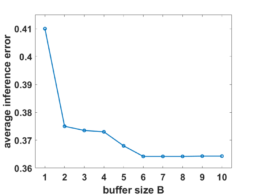
(b) $\sigma=\frac{5}{2}$

Figure 7: Time-average inference error vs. the buffer size B for ${\sigma=\frac{1}{2}}$ and ${\sigma=\frac{5}{2}}$.

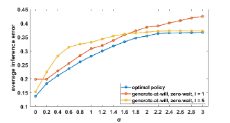
Figure 8: Time-average inference error vs. the scaling parameter $\sigma$ of transmission delay $T_{i}(l)$.

Fig. 7(a) and Fig. 7(b) show the time-average inference error achieved by the optimal policy in Theorem 2 for buffer size values $B$, ranging from $1$ to $10$, with ${\sigma=\frac{1}{2}}$ and ${\sigma=\frac{5}{2}}$, respectively. As the buffer size increases, the performance improvement diminishes and becomes less significant. Therefore, we fix the buffer size $B$ at $10$ for this experiment.

Fig. 8 presents the time-average inference error achieved by the following three scheduling policies as the parameter $\sigma$ changes from $0$ to $3$:

• Optimal policy in Theorem 2

• Generate-at-will, zero-wait, $l=1$ policy: $(f,\ell,g)$ such that $f=g=(0,0,\ldots)$ and $\ell=(1,1,\ldots)$.

• Generate-at-will, zero-wait, $l=5$ policy: $(f,\ell,g)$ such that $f=g=(0,0,\ldots)$ and $\ell=(5,5,\ldots)$.

The result in Fig. 8 highlights the importance of adjusting the packet length over time in response to varying delay conditions. The optimal policy in Theorem 2 outperforms the other two policies, which use constant packet length, achieving up to $25\%$ reduction in average inference error.

VI Conclusion

This paper studies a goal-oriented communication design problem for remote inference, where an intelligent model on the receiver side predicts the real-time value of a target signal using data packets transmitted from a remote location. We derive two optimal scheduling policies under time-invariant and time-variable packet length selection. These policies minimize the expected time-average inference error for a possibly non-monotonic inference error function by considering the interplay between packet length and transmission delay, as well as by exploiting delay memory. Finally, through the simulations, we demonstrate the significant benefits of adopting such a goal-oriented communication strategy for remote inference.

Appendix A

The SMDP corresponding to problem (6), constructed in Section III-B, is described by the following components [21]:

(i) Decision Time: Each ACK reception time slot $A_{i}=S_{i}+T_{i}(l)+F_{i}$ is a decision time.

(ii) Action: At each decision time $A_{i}$, the scheduler determines the waiting time $\tau_{i+1}$ and buffer position $b_{i+1}$ for the next packet to be transmitted.

(iii) State and State Transitions: The system state at each decision time $A_{i}$ is represented by the tuple $\big{(}\delta,c_{i}\big{)}$, where $\delta=\Delta(A_{i})$ and $c_{i}$ is the delay state in the $i$-th epoch. The AoI $\Delta(t)$ at time slot $t$ evolves according to equation (1). Meanwhile, the delay state $C_{i}=c_{i}$ in the $i$-th epoch evolves according to the finite-state ergodic Markov chain defined in Section (II). The Markov chain makes a single transition at each decision time $A_{i}$ and none otherwise.

(iv) Transition Time and Cost: The time between the consecutive decision times $A_{i+1}-A_{i}$ is represented by the random variable $\tau_{i+1}+T_{i+1}(l)+F_{i+1}$, given the delay state $C_{i}=c_{i}$. Moreover, the cost incurred while transitioning from decision time $A_{i}$ to decision time $A_{i+1}$,

$$\sum_{t=A_{i}}^{A_{i+1}-1}\varepsilon\big{(}\Delta(t),l\big{)},$$

is represented by the random variable

$$\sum_{k=0}^{\tau_{i+1}+T_{i+1}(l)-1}\varepsilon\big{(}\Delta(A_{i})+k,l\big{)}+\sum_{k=0}^{F_{i+1}-1}\varepsilon\big{(}b_{i+1}+T_{i+1}(l)+k,l\big{)},$$

given the delay state $C_{i}=c_{i}$.

Appendix B Proof of Theorem 1

This proof consists of three steps.

Step 1: We prove two structural results regarding the optimal scheduling policy by using the Bellman optimality equation (III-B), which comprises three terms. The first term,

$$\mathbb{E}\Bigg{[}\sum_{k=0}^{\tau_{i+1}+T_{i+1}(l)-1}\bigg{(}\varepsilon\big{(}\delta+k,l\big{)}-\varepsilon_{l,\text{opt}}\bigg{)}\Bigg{|}C_{i}=c_{i}\Bigg{]},$$

is independent of the buffer position $b_{i+1}$. In contrast, the remaining two terms,

$$\mathbb{E}\Bigg{[}\sum_{k=0}^{F_{i+1}-1}\bigg{(}\varepsilon\big{(}b_{i+1}+T_{i+1}(l)+k,l\big{)}-\varepsilon_{l,\text{opt}}\bigg{)}\Bigg{|}C_{i}=c_{i}\Bigg{]}$$

and

$$\mathbb{E}\bigg{[}h_{1}\big{(}b_{i+1}+T_{i+1}(l)+F_{i+1},C_{i+1}\big{)}\bigg{|}C_{i}=c_{i}\bigg{]},$$

are independent of the waiting time $\tau_{i+1}$. Consequently, the optimal buffer position $b_{i+1}^{*}$ and the optimal waiting time $\tau_{i+1}^{*}$ can be determined by solving separate optimization problems.

(i) Optimal Waiting Time: The optimal waiting time $\tau_{i+1}^{*}$, when $\Delta(A_{i})=\delta$ and $C_{i}=c_{i}$, can be determined by solving the optimization problem

$$\min_{\tau_{i+1}\in\{0,1,\ldots\}}\mathbb{E}\Bigg{[}\sum_{k=0}^{\tau_{i+1}+T_{i+1}(l)-1}\bigg{(}\varepsilon\big{(}\delta+k,l\big{)}-\varepsilon_{l,\text{opt}}\bigg{)}\Bigg{|}C_{i}=c_{i}\Bigg{]}.$$ (21)

Problem (21) is a simple integer optimization problem. The optimal waiting time $\tau_{i+1}^{*}=0$ if

$$\min_{\tau_{i+1}\in\{1,2,\ldots\}} \mathbb{E}\Bigg{[}\sum_{k=0}^{\tau_{i+1}+T_{i+1}(l)-1}\bigg{(}\varepsilon\big{(}\delta+k,l\big{)}-\varepsilon_{l,\text{opt}}\bigg{)}\Bigg{|}C_{i}=c_{i}\Bigg{]}\geq$$

$$\mathbb{E}\Bigg{[}\sum_{k=0}^{T_{i+1}(l)-1}\bigg{(}\varepsilon\big{(}\delta+k,l\big{)}-\varepsilon_{l,\text{opt}}\bigg{)}\Bigg{|}C_{i}=c_{i}\Bigg{]}.$$ (22)

By some algebraic manipulations, we can obtain

$$\min_{\tau_{i+1}\in\{1,2,\ldots\}}\mathbb{E}\Bigg{[}\sum_{k=0}^{\tau_{i+1}-1}\bigg{(}\varepsilon\big{(}\delta+T_{i+1}(l)+k,l\big{)}-\varepsilon_{l,\text{opt}}\bigg{)}\Bigg{|}C_{i}=c_{i}\Bigg{]}$$

$$\geq 0.$$ (23)

The inequality (B) holds if and only if

$$\min_{\tau_{i+1}\in\{1,2,\ldots\}}\frac{1}{\tau_{i+1}}\sum_{k=0}^{\tau_{i+1}-1}\mathbb{E}\bigg{[}\varepsilon\big{(}\delta+T_{i+1}(l)+k,l\big{)}\bigg{|}C_{i}=c_{i}\bigg{]}\geq\varepsilon_{l,\text{opt}}.$$ (24)

The left-hand side of (24) is equal to $\gamma\big{(}\delta,l,l,c_{i}\big{)}$, where $\gamma\big{(}\cdot\big{)}$ is the index function defined in (9). Similarly, the optimal waiting time $\tau_{i+1}^{*}=1$, if $\tau_{i+1}^{*}\neq 0$ and

$$\min_{\tau_{i+1}\in\{2,3,\ldots\}}\mathbb{E}\Bigg{[}\sum_{k=1}^{\tau_{i+1}-1}\bigg{(}\varepsilon\big{(}\delta+T_{i+1}(l)+k,l\big{)}-\varepsilon_{l,\text{opt}}\bigg{)}\Bigg{|}C_{i}=c_{i}\Bigg{]}$$

$$\geq 0.$$ (25)

Following the same steps in (B)-(24), we can demonstrate that the inequality (B) is equivalent to

$$\gamma\big{(}\delta+1,l,l,c_{i}\big{)}\geq\varepsilon_{l,\text{opt}}.$$ (26)

By repeating (B)-(26), we can establish the rule that the optimal waiting time $\tau_{i+1}^{*}$ is equal to $k$, provided that ${\tau_{i+1}^{*}\neq 0,1,\ldots,k-1}$ and

$$\gamma\big{(}\delta+k,l,l,c_{i}\big{)}\geq\varepsilon_{l,\text{opt}}.$$ (27)

Hence, any $\tau_{i+1}^{*}$ in the optimal waiting time sequence ${g^{*}=\big{(}\tau_{2}^{*},\tau_{3}^{*},\ldots\big{)}}$ is determined by the index-based threshold rule $\tau_{l}\big{(}\delta,c_{i}\big{)}$ given by equation (10).

(ii) Optimal Buffer Position: The optimal buffer position $b_{i+1}^{*}$, when $\Delta(A_{i})=\delta$ and $C_{i}=c_{i}$, can be determined by solving the optimization problem

$$\min_{b_{i+1}\in\{0,1,\ldots,B-l\}}$$

$$\mathbb{E}\Bigg{[}\sum_{k=0}^{F_{i+1}-1}\bigg{(}\varepsilon\big{(}b_{i+1}+T_{i+1}(l)+k,l\big{)}-\varepsilon_{l,\text{opt}}\bigg{)}\Bigg{|}C_{i}=c_{i}\Bigg{]}$$

$$+\mathbb{E}\bigg{[}h_{1}\big{(}b_{i+1}+T_{i+1}(l)+F_{i+1},C_{i+1}\big{)}\bigg{|}C_{i}=c_{i}\bigg{]}.$$ (28)

From (B), we observe that the optimal buffer position $b_{i+1}^{*}$ is independent of $\delta=\Delta(A_{i})$ and depends only on the delay state $c_{i}$ in the previous epoch. In other words, $c_{i}$ is a sufficient statistic for determining $b_{i+1}^{*}$ for all $i$.

Step 2: We construct a new SMDP based on the results obtained in the first step. In the new SMDP, the decision time is $D_{i+1}$ instead of $A_{i}$. At each decision time $D_{i+1}$, the system state is represented only by the delay state $c_{i}$ in the $i$-th epoch. We fix the waiting time decisions by using optimal threshold rule $\tau_{l}\big{(}\delta,c_{i}\big{)}$, and the action involves determining the buffer position $b_{i+1}$. A detailed description of this SMDP can be found in Appendix D. The Bellman optimality equation of this new SMDP is given by equation (III-B).

The second term on the right-hand side of equation (III-B),

$$\mathbb{E}\bigg{[}h_{1}^{\prime}\big{(}C_{i+1}\big{)}\bigg{|}C_{i}=c\bigg{]},$$

is independent of the action $b_{i+1}$ taken at decision time $D_{i+1}$ and depends only on the state $C_{i}=c_{i}$. Therefore, the Bellman optimality equation (III-B) is decomposable and can be solved as a per-decision epoch optimization problem; that is, we can express any $b_{i+1}^{*}$ in the optimal buffer position sequence ${f^{*}=\big{(}b_{2}^{*},b_{3}^{*},\ldots\big{)}}$ as shown in (1).

Step 3: We determine the optimal value $\varepsilon_{l,\text{opt}}$ of the inner optimization problem (6) as the unique root of equation (12). Let $\vartheta_{i}^{*}$ denote the random variable $b_{i}^{*}+T_{i}(l)+F_{i}$. Consider the following equality:

$$\mathbb{E}\Bigg{[}\sum_{t=A_{i}}^{A_{i+1}-1}\varepsilon\big{(}\Delta(t)\big{)}\Bigg{]}-\varepsilon_{l,\text{opt}}\mathbb{E}\big{[}A_{i+1}-A_{i}\big{]}=$$

$$\mathbb{E}\Bigg{[}\sum_{k=0}^{\tau_{l}\big{(}\vartheta_{i}^{*},C_{i}\big{)}+T_{i+1}(l)-1}\bigg{(}\varepsilon\big{(}\vartheta_{i}^{*}+k,l\big{)}-\varepsilon_{l,\text{opt}}\bigg{)}\Bigg{]}$$

$$+\mathbb{E}\Bigg{[}\sum_{k=0}^{F_{i+1}-1}\bigg{(}\varepsilon\big{(}b_{i+1}^{*}+T_{i+1}(l)+k,l\big{)}-\varepsilon_{l,\text{opt}}\bigg{)}\Bigg{]}.$$ (29)

We first demonstrate that the right-hand side of equation (B) is equal to zero, which implies $\varepsilon_{l,\text{opt}}$ is indeed a root of equation (12). From the Bellman equation (III-B), we can obtain the following relation:

$$h_{1}\big{(}\vartheta_{i}^{*},C_{i}\big{)}=$$

$$\mathbb{E}\Bigg{[}\sum_{k=0}^{\tau_{l}\big{(}\vartheta_{i}^{*},C_{i}\big{)}+T_{i+1}(l)-1}\bigg{(}\varepsilon\big{(}\vartheta_{i}^{*}+k,l\big{)}-\varepsilon_{l,\text{opt}}\bigg{)}\Bigg{|}C_{i}\Bigg{]}$$

$$+\mathbb{E}\Bigg{[}\sum_{k=0}^{F_{i+1}-1}\bigg{(}\varepsilon\big{(}b_{i+1}^{*}+T_{i+1}(l)+k,l\big{)}-\varepsilon_{l,\text{opt}}\bigg{)}\Bigg{|}C_{i}\Bigg{]}$$

$$+\mathbb{E}\bigg{[}h_{1}\big{(}\vartheta_{i+1}^{*},C_{i+1}\big{)}\bigg{|}C_{i}\bigg{]}.$$ (30)

By the law of iterated expectations, taking the expectation over $C_{i}$ on both sides of (B) gives us the equation

$$\mathbb{E}\big{[}h_{1}\big{(}\vartheta_{i}^{*},C_{i}\big{)}\big{]}=$$

$$\mathbb{E}\Bigg{[}\sum_{k=0}^{\tau_{l}\big{(}\vartheta_{i}^{*},C_{i}\big{)}+T_{i+1}(l)-1}\bigg{(}\varepsilon\big{(}\vartheta_{i}^{*}+k,l\big{)}-\varepsilon_{l,\text{opt}}\bigg{)}\Bigg{]}$$

$$+\mathbb{E}\Bigg{[}\sum_{k=0}^{F_{i+1}-1}\bigg{(}\varepsilon\big{(}b_{i+1}^{*}+T_{i+1}(l)+k,l\big{)}-\varepsilon_{l,\text{opt}}\bigg{)}\Bigg{]}$$

$$+\mathbb{E}\big{[}h_{1}\big{(}\vartheta_{i+1}^{*},C_{i+1}\big{)}\big{]}.$$ (31)

Since $C_{i}$ evolves according to an ergodic Markov chain with a unique stationary distribution, it follows that $\mathbb{E}\big{[}h_{1}\big{(}\vartheta_{i}^{*},C_{i}\big{)}\big{]}=\mathbb{E}\big{[}h_{1}\big{(}\vartheta_{i+1}^{*},C_{i+1}\big{)}\big{]}$. Therefore, equation (B) implies that the right-hand side of equation (B) is equal to zero.

Next, we prove the uniqueness of the root $\varepsilon_{l,\text{opt}}$. The right-hand side of equation (B) can be written as

$$\min_{\tau\big{(}\cdot\big{)}}\text{ }\mathbb{E}\Bigg{[}\sum_{k=0}^{\tau\big{(}\vartheta_{i}^{*},C_{i}\big{)}+T_{i+1}(l)-1}\bigg{(}\varepsilon\big{(}\vartheta_{i}^{*}+k,l\big{)}-\varepsilon_{l,\text{opt}}\bigg{)}\Bigg{]}$$

$$+\mathbb{E}\Bigg{[}\sum_{k=0}^{F_{i+1}-1}\bigg{(}\varepsilon\big{(}b_{i+1}^{*}+T_{i+1}(l)+k,l\big{)}-\varepsilon_{l,\text{opt}}\bigg{)}\Bigg{]}.$$ (32)

The expression in (B) is concave, continuous, and strictly decreasing in $\varepsilon_{l,\text{opt}}$, as the first term is the functional minimum of linear decreasing functions of $\varepsilon_{l,\text{opt}}$, and the second term is itself a linear decreasing function of $\varepsilon_{l,\text{opt}}$. Therefore, since

$$\lim_{\varepsilon_{l,\text{opt}}\to\infty}\mathbb{E}\Bigg{[}\sum_{k=0}^{\tau\big{(}\vartheta_{i}^{*},C_{i}\big{)}+T_{i+1}(l)-1}\bigg{(}\varepsilon\big{(}\vartheta_{i}^{*}+k,l\big{)}-\varepsilon_{l,\text{opt}}\bigg{)}\Bigg{]}=-\infty$$

and

$$\lim_{\varepsilon_{l,\text{opt}}\to-\infty}\mathbb{E}\Bigg{[}\sum_{k=0}^{\tau\big{(}\vartheta_{i}^{*},C_{i}\big{)}+T_{i+1}(l)-1}\bigg{(}\varepsilon\big{(}\vartheta_{i}^{*}+k,l\big{)}-\varepsilon_{l,\text{opt}}\bigg{)}\Bigg{]}=\infty$$

for any $\tau\big{(}\cdot\big{)}$, and

$$\lim_{\varepsilon_{l,\text{opt}}\to\infty}\mathbb{E}\Bigg{[}\sum_{k=0}^{F_{i+1}-1}\bigg{(}\varepsilon\big{(}b_{i+1}^{*}+T_{i+1}(l)+k,l\big{)}-\varepsilon_{l,\text{opt}}\bigg{)}\Bigg{]}=-\infty$$

and

$$\lim_{\varepsilon_{l,\text{opt}}\to-\infty}\mathbb{E}\Bigg{[}\sum_{k=0}^{F_{i+1}-1}\bigg{(}\varepsilon\big{(}b_{i+1}^{*}+T_{i+1}(l)+k,l\big{)}-\varepsilon_{l,\text{opt}}\bigg{)}\Bigg{]}=\infty,$$

equation (12) has a unique root. This completes the proof.

Appendix C

The SMDP corresponding to problem (14), constructed in Section IV-B, is described by the following components [21]:

(i) Decision Time: Each ACK reception time slot $A_{i}=S_{i}+T_{i}(l_{i})+F_{i}$ is a decision time.

(ii) Action: At each decision time $A_{i}$, the scheduler determines the waiting time $\tau_{i+1}$, packet length $l_{i+1}$, and buffer position $b_{i+1}$ for the next packet to be transmitted.

(iii) State and State Transitions: The system state at each decision time $A_{i}$ is represented by the tuple $\big{(}\delta,d,c_{i}\big{)}$, where $\delta=\Delta(A_{i})$, $d=d(A_{i})$, and $c_{i}$ is the delay state in the $i$-th epoch. The AoI $\Delta(t)$ at time slot $t$ and the length $d(t)$ of the packet most recently delivered by time slot $t$ evolve according to equations (1) and (2), respectively. Meanwhile, the delay state $C_{i}=c_{i}$ in the $i$-th epoch evolves according to the finite-state ergodic Markov chain defined in Section (II). The Markov chain makes a single transition at each decision time $A_{i}$ and none otherwise.

(iv) Transition Time and Cost: The time between the consecutive decision times $A_{i+1}-A_{i}$ is represented by the random variable $\tau_{i+1}+T_{i+1}(l_{i+1})+F_{i+1}$, given the delay state $C_{i}=c_{i}$. Moreover, the cost incurred while transitioning from decision time $A_{i}$ to decision time $A_{i+1}$,

$$\sum_{t=A_{i}}^{A_{i+1}-1}\varepsilon\big{(}\Delta(t),d(t)\big{)},$$

is represented by the random variable

$$\sum_{k=0}^{\tau_{i+1}+T_{i+1}(l_{i+1})-1}\varepsilon\big{(}\Delta(A_{i})+k,d(A_{i})\big{)}$$

$$+\sum_{k=0}^{F_{i+1}-1}\varepsilon\big{(}b_{i+1}+T_{i+1}(l_{i+1})+k,l_{i+1}\big{)},$$

given the delay state $C_{i}=c_{i}$.

Appendix D

The components of the SMDP constructed in the second step of the proof of Theorem (1) differ from those of the SMDPs constructed in Sections III-B and IV-B.

(i) Decision Time: Each delivery time slot $D_{i+1}=S_{i+1}+T_{i+1}(l)$ is a decision time.

(ii) Action: At each decision time $D_{i+1}$, the scheduler determines the buffer position $b_{i+1}$ for the next packet to be transmitted.

(iii) State and State Transitions: The system state at each decision time $D_{i+1}$ is the delay state $C_{i}=c_{i}$ in the $i$-th epoch, which evolves according to the finite-state ergodic Markov chain defined in Section (II). The Markov chain makes a single transition at each decision time $A_{i}$ and none otherwise.

(iv) Transition Time and Cost: The time between consecutive decision times, $D_{i+1}-D_{i}$, is represented by the random variable $\vartheta_{i+1}=F_{i+1}+\tau_{l}\big{(}b_{i+1}+T_{i+1}(l)+F_{i+1},C_{i+1}\big{)}+T_{i+2}(l)$, given the delay state $C_{i}=c_{i}$, where $\tau_{l}\big{(}\cdot\big{)}$ is the waiting time rule defined in (10). Moreover, the cost incurred while transitioning from decision time $D_{i}$ to decision time $D_{i+1}$,

$$\sum_{t=D_{i}}^{D_{i+1}-1}\varepsilon\big{(}\Delta(t),l\big{)},$$

is represented by the random variable

$$\sum_{k=0}^{\vartheta_{i+1}-1}\varepsilon\big{(}b_{i+1}+T_{i+1}(l)+k,l\big{)},$$

given the delay state $C_{i}=c_{i}$.

Appendix E Proof of Theorem 2

The Bellman optimality equation in (IV-B) has three terms. The first term,

$$\mathbb{E}\Bigg{[}\sum_{k=0}^{\tau_{i+1}+T_{i+1}(l_{i+1})-1}\bigg{(}\varepsilon\big{(}\delta+k,d\big{)}-\varepsilon_{\text{opt}}\bigg{)}\Bigg{|}C_{i}=c_{i}\Bigg{]},$$

does not depend on the buffer position $b_{i+1}$. On the contrary, the remaining two terms,

$$\mathbb{E}\Bigg{[}\sum_{k=0}^{F_{i+1}-1}\bigg{(}\varepsilon\big{(}b_{i+1}+T_{i+1}(l_{i+1})+k,l_{i+1}\big{)}-\varepsilon_{\text{opt}}\bigg{)}\Bigg{|}C_{i}=c_{i}\Bigg{]}$$

and

$$\mathbb{E}\big{[}h_{2}\big{(}b_{i+1}+T_{i+1}(l_{i+1})+F_{i+1},l_{i+1},C_{i+1}\big{)}\big{|}C_{i}=c_{i}\big{]},$$

do not depend on the waiting time $\tau_{i+1}$. Therefore, given the optimal packet length $l_{i+1}^{*}$, the optimal waiting time $\tau_{i+1}^{*}$, when $\Delta(A_{i})=\delta$, $d(A_{i})=d$, and $C_{i}=c_{i}$, can be determined by solving the following optimization problem, which is independent of the action $b_{i+1}$:

$$\min_{\tau_{i+1}\in\{0,1,\ldots\}}\mathbb{E}\Bigg{[}\sum_{k=0}^{\tau_{i+1}+T_{i+1}(l_{i+1}^{*})-1}\bigg{(}\varepsilon\big{(}\delta+k,d\big{)}-\varepsilon_{\text{opt}}\bigg{)}\Bigg{|}C_{i}=c_{i}\Bigg{]}.$$ (33)

Problem (33) is a simple integer optimization problem, quite similar to problem (21). By following the steps in (B) through (26), we can show that the optimal waiting time $\tau_{i+1}^{*}=k$, if $\tau_{i+1}^{*}\neq 0,1,\ldots,k-1$ and

$$\gamma(\delta+k,d,l_{i+1}^{*},c_{i})\geq\varepsilon_{\text{opt}},$$ (34)

where $\gamma\big{(}\cdot\big{)}$ is the index function defined in (9). Hence, the optimal waiting time $\tau_{i+1}^{*}$ is determined as given in equation (16), and the Bellman optimality equation (IV-B) can be equivalently formulated as (2). This completes the proof.

References

- [1] C. Ari, M. K. C. Shisher, E. Uysal, and Y. Sun, “Goal-oriented communications for remote inference under two-way delay with memory,” in IEEE ISIT, 2024, pp. 1179–1184.
- [2] B. Smith, “From Simulation to Reality: How Digital Twins Are Transforming the Space Industry,” https://www.nominalsys.com/blogs/what-is-a-digital-twin, 2023, [Online; accessed 13-May-2023].
- [3] L. Zhao, C. Wang, K. Zhao, D. Tarchi, S. Wan, and N. Kumar, “INTERLINK: A Digital Twin-Assisted Storage Strategy for Satellite-Terrestrial Networks,” IEEE Transactions on Aerospace and Electronic Systems, vol. 58, no. 5, pp. 3746–3759, 2022.
- [4] M. K. C. Shisher and Y. Sun, “How does data freshness affect real-time supervised learning?” in ACM MobiHoc, 2022, pp. 31–40.
- [5] M. K. C. Shisher, Y. Sun, and I.-H. Hou, “Timely communications for remote inference,” IEEE/ACM Transactions on Networking, 2024, in press.
- [6] E. Uysal, “Goal-oriented communications for interplanetary and non-terrestrial networks,” arXiv preprint arXiv:2409.14534, 2024.
- [7] W. Weaver, “The mathematics of communication,” Scientific American, vol. 181, no. 4, pp. 11–15, 1949.
- [8] E. Uysal, O. Kaya, A. Ephremides, J. Gross, M. Codreanu, P. Popovski, M. Assaad, G. Liva, A. Munari, B. Soret et al., “Semantic communications in networked systems: A data significance perspective,” IEEE Network, vol. 36, no. 4, pp. 233–240, 2022.
- [9] Q. Voortman, D. Efimov, A. Pogromsky, J.-P. Richard, and H. Nijmeijer, “Remote state estimation of steered systems with limited communications: an event-triggered approach,” IEEE Transactions on Automatic Control, 2023.
- [10] Y. E. Sagduyu, T. Erpek, A. Yener, and S. Ulukus, “Multi-receiver task-oriented communications via multi-task deep learning,” in IEEE FNWF, 2023, pp. 1–6.
- [11] M. Merluzzi, M. C. Filippou, L. G. Baltar, and E. C. Strinati, “Effective goal-oriented 6g communications: The energy-aware edge inferencing case,” in Joint European Conference on Networks and Communications & 6G Summit. IEEE, 2022, pp. 457–462.
- [12] P. Talli, F. Pase, F. Chiariotti, A. Zanella, and M. Zorzi, “Semantic and effective communication for remote control tasks with dynamic feature compression,” in IEEE INFOCOM Workshops, 2023, pp. 1–6.
- [13] F. Peng, X. Wang, and X. Chen, “Online learning of goal-oriented status updating with unknown delay statistics,” IEEE Journal on Selected Areas in Communications, 2024.
- [14] A. Li, S. Wu, S. Sun, and J. Cao, “Goal-oriented tensor: Beyond age of information towards semantics-empowered goal-oriented communications,” IEEE Transactions on Communications, 2024.
- [15] S. Kaul, R. Yates, and M. Gruteser, “Real-time status: How often should one update?” in IEEE INFOCOM, 2012, pp. 2731–2735.
- [16] Y. Sun, Y. Polyanskiy, and E. Uysal, “Sampling of the wiener process for remote estimation over a channel with random delay,” IEEE Transactions on Information Theory, vol. 66, no. 2, pp. 1118–1135, 2019.
- [17] M. K. C. Shisher, B. Ji, I.-H. Hou, and Y. Sun, “Learning and communications co-design for remote inference systems: Feature length selection and transmission scheduling,” IEEE Journal on Selected Areas in Information Theory, 2023.
- [18] R. D. Yates, “Lazy is timely: Status updates by an energy harvesting source,” in IEEE ISIT, 2015, pp. 3008–3012.
- [19] Y. Sun, E. Uysal-Biyikoglu, R. D. Yates, C. E. Koksal, and N. B. Shroff, “Update or wait: How to keep your data fresh,” IEEE Transactions on Information Theory, vol. 63, no. 11, pp. 7492–7508, 2017.
- [20] M. L. Puterman, Markov decision processes: discrete stochastic dynamic programming. John Wiley & Sons, 2014.
- [21] D. Bertsekas, Dynamic programming and optimal control: Volume I. Athena scientific, 2012, vol. 4.
- [22] M. K. C. Shisher, H. Qin, L. Yang, F. Yan, and Y. Sun, “The age of correlated features in supervised learning based forecasting,” in IEEE INFOCOM Workshops, 2021, pp. 1–8.
- [23] I. Kadota, A. Sinha, and E. Modiano, “Optimizing age of information in wireless networks with throughput constraints,” in IEEE INFOCOM, 2018, pp. 1844–1852.
- [24] Y. Sun and B. Cyr, “Sampling for data freshness optimization: Non-linear age functions,” Journal of Communications and Networks, vol. 21, no. 3, pp. 204–219, 2019.
- [25] T. Z. Ornee and Y. Sun, “Sampling and remote estimation for the ornstein-uhlenbeck process through queues: Age of information and beyond,” IEEE/ACM Transactions on Networking, vol. 29, no. 5, pp. 1962–1975, 2021.
- [26] V. Tripathi and E. Modiano, “A whittle index approach to minimizing functions of age of information,” in 57th Annual Allerton Conference on Communication, Control, and Computing. IEEE, 2019, pp. 1160–1167.
- [27] M. Klügel, M. H. Mamduhi, S. Hirche, and W. Kellerer, “Aoi-penalty minimization for networked control systems with packet loss,” in IEEE INFOCOM Workshops, 2019, pp. 189–196.
- [28] J. Sun, Z. Jiang, B. Krishnamachari, S. Zhou, and Z. Niu, “Closed-form whittle’s index-enabled random access for timely status update,” IEEE Transactions on Communications, vol. 68, no. 3, pp. 1538–1551, 2019.
- [29] T. Z. Ornee and Y. Sun, “A Whittle index policy for the remote estimation of multiple continuous Gauss-Markov processes over parallel channels,” ACM MobiHoc, 2023.
- [30] J. Pan, Y. Sun, and N. B. Shroff, “Sampling for remote estimation of the wiener process over an unreliable channel,” ACM Sigmetrics, 2023.
- [31] T. Z. Ornee, M. K. C. Shisher, C. Kam, and Y. Sun, “Context-aware status updating: Wireless scheduling for maximizing situational awareness in safety-critical systems,” in IEEE MILCOM, 2023, pp. 194–200.
- [32] M. K. C. Shisher and Y. Sun, “On the monotonicity of information aging,” IEEE INFOCOM ASoI Workshop, 2024.
- [33] A. M. Bedewy, Y. Sun, R. Singh, and N. B. Shroff, “Optimizing information freshness using low-power status updates via sleep-wake scheduling,” in ACM MobiHoc, 2020, pp. 51–60.
- [34] A. M. Bedewy, Y. Sun, S. Kompella, and N. B. Shroff, “Optimal sampling and scheduling for timely status updates in multi-source networks,” IEEE Transactions on Information Theory, vol. 67, no. 6, pp. 4019–4034, 2021.
- [35] R. D. Yates, Y. Sun, D. R. Brown, S. K. Kaul, E. Modiano, and S. Ulukus, “Age of information: An introduction and survey,” IEEE Journal on Selected Areas in Communications, vol. 39, no. 5, pp. 1183–1210, 2021.
- [36] T. Soleymani, J. S. Baras, and K. H. Johansson, “Stochastic control with stale information–part i: Fully observable systems,” in IEEE CDC, 2019, pp. 4178–4182.
- [37] B. T. Bacinoglu, E. T. Ceran, and E. Uysal-Biyikoglu, “Age of information under energy replenishment constraints,” in IEEE ITA, 2015, pp. 25–31.
- [38] I. Kadota, A. Sinha, E. Uysal-Biyikoglu, R. Singh, and E. Modiano, “Scheduling policies for minimizing age of information in broadcast wireless networks,” IEEE/ACM Transactions on Networking, vol. 26, no. 6, pp. 2637–2650, 2018.
- [39] I. Kadota, A. Sinha, and E. Modiano, “Scheduling algorithms for optimizing age of information in wireless networks with throughput constraints,” IEEE/ACM Transactions on Networking, vol. 27, no. 4, pp. 1359–1372, 2019.
- [40] C.-H. Tsai and C.-C. Wang, “Unifying aoi minimization and remote estimation—optimal sensor/controller coordination with random two-way delay,” IEEE/ACM Transactions on Networking, vol. 30, no. 1, pp. 229–242, 2021.
- [41] J. Pan, A. M. Bedewy, Y. Sun, and N. B. Shroff, “Optimal sampling for data freshness: Unreliable transmissions with random two-way delay,” IEEE/ACM Transactions on Networking, vol. 31, no. 1, pp. 408–420, 2022.
- [42] I. Goodfellow, “Deep learning,” 2016.
- [43] T. N. Pham, S. Nahavandi, H. Trinh, K. P. Wong et al., “Static output feedback frequency stabilization of time-delay power systems with coordinated electric vehicles state of charge control,” IEEE Transactions on Power Systems, vol. 32, no. 5, pp. 3862–3874, 2016.
- [44] C. Briat, O. Sename, and J.-F. Lafay, “Memory-resilient gain-scheduled state-feedback control of uncertain lti/lpv systems with time-varying delays,” Systems and Control Letters, vol. 59, no. 8, pp. 451–459, 2010.
- [45] V. Léchappé, E. Moulay, and F. Plestan, “Dynamic observation-prediction for lti systems with a time-varying delay in the input,” in IEEE CDC, 2016, pp. 2302–2307.
- [46] K. T. Truong and R. W. Heath, “Effects of channel aging in massive mimo systems,” Journal of Communications and Networks, vol. 15, no. 4, pp. 338–351, 2013.
- [47] G. Brockman, V. Cheung, L. Pettersson, J. Schneider, J. Schulman, J. Tang, and W. Zaremba, “Openai gym,” arXiv:1606.01540, 2016.
- [48] V. Mnih, K. Kavukcuoglu, D. Silver et al., “Human-level control through deep reinforcement learning,” nature, vol. 518, no. 7540, pp. 529–533, 2015.