Two-Dimensional Active Brownian Particles Crossing a Parabolic Barrier:
Transition-Path Times, Survival Probability, and First-Passage time.

Abstract

We derive an analytical expression for the propagator and the transition path time distribution of a two-dimensional active Brownian particle crossing a parabolic barrier with absorbing boundary conditions at both sides. Using the passive Brownian particle as basis states and dealing with the activity as a perturbation, our solution is expressed in terms of the perturbed eigenfunctions and eigenvalues of the associated Fokker-Planck equation once the latter is reduced by taking into account only the coordinate along the direction of the barrier and the self-propulsion angle. We show that transition path times are typically shortened by the self-propulsion of the particle. Our solution also allows us to obtain the survival probability and the first-passage time distribution, which display a strong dependence on the particle’s activity, while the rotational diffusivity influences them to a minor extent.

Introduction

Active particles are characterized by the ability to consume energy from their environment in order to generate self-propelled directed motion Bechinger et al. (2016); Marchetti et al. (2013); Romanczuk et al. (2012); Elgeti et al. (2015). Recent decades have seen significant and growing effort in investigating their dynamics because of their relevance in a wide variety of fields including biology Needleman and Dogic (2017); Lipowsky and Klumpp (2005), biomedicine Wang and Gao (2012); Henkes et al. (2020), robotics Cheang et al. (2014); Erkoc et al. (2019), social transport Helbing (2001), and statistical physics Cates (2012); Chaudhuri (2014); Fodor et al. (2016); Falasco et al. (2016); Speck (2016); Fodor and Marchetti (2018); Caraglio and Franosch (2022).

For systems of interacting active particles novel emerging collective behavior arises Kumar et al. (2014); Fily and Marchetti (2012); Slowman et al. (2016); Stenhammar et al. (2015). Furthermore, even at the single particle level, self-propelled particles show remarkable features like, for example, accumulation near confining boundaries Elgeti and Gompper (2013); Volpe et al. (2014), non-Boltzmann stationary distribution Tailleur and Cates (2009); Malakar et al. (2018); Wagner et al. (2017); Malakar et al. (2020), and oscillating intermediate scattering function Kurzthaler et al. (2016); Kurzthaler and Franosch (2017); Kurzthaler et al. (2018). However, notwithstanding the tremendous progress that happened in this research field in the past decade, exactly solvable models, allowing a deeper understanding of some basic theoretical aspects, remain rare. Exceptions include active Brownian particles (ABPs) in channels Wagner et al. (2017) or sedimenting in a gravitational field Hermann and Schmidt (2018) and run-and-tumble particles in one dimension Schnitzer (1993); Tailleur and Cates (2008, 2009); Malakar et al. (2018). The analytical solution of the time-dependent probability distribution of run-and-tumble and ABPs in free space is known only in the Fourier domain Kurzthaler et al. (2016); Kurzthaler and Franosch (2017); Kurzthaler et al. (2018); Martens et al. (2012); Sevilla and Sandoval (2015). More recently, the steady-state distribution of a two-dimensional ABP trapped in an isotropic harmonic potential has been derived Malakar et al. (2020) and its time-dependent Fokker-Planck equation has been fully solved Caraglio and Franosch (2022). Finally, the Fokker-Planck equation has been solved also for an ABP exploring a circular region with an absorbing boundary Di Trapani et al. (2023).

Here, we extend even more the set of solvable models by considering an ABP navigating in a domain characterized a parabolic barrier along one direction and presenting absorbing boundaries at both sides of the barrier. Building upon the theory developed in Ref.s Caraglio and Franosch (2022); Di Trapani et al. (2023), we show that also in the current system a formally exact series expression for the probability propagator associated to the Fokker-Planck equation can be obtained once the basis states of a reference standard Brownian particle are known. For the considered environment, we attain the basis states of a passive Brownian particle by extending to two dimensions the solution of the Fokker-Planck equation for a one-dimensional particle crossing a parabolic barrier as achieved in Ref. Caraglio et al. (2018). In the companion paper Caraglio (2024), we solve the case of a rectangular domain delimited by an absorbing boundary in each direction. In the present manuscript, we rather focus on the case of a domain infinitely extended in the direction perpendicular to the energy barrier and we found an expression for the reduced propagator taking into account the position along the direction of the barrier and the self-propulsion angle but not the position along the perpendicular direction.

Furthermore, again taking inspiration from Ref. Caraglio et al. (2018), we also derive an expression for the transition-path-times (TPTs) distribution. In a barrier-crossing process, transition paths are defined as those trajectories originating on a point at one side of the barrier and ending at another point at the opposite side, without recrossing the initial position. In the context of passive dynamics, both experimentalists Chung et al. (2009); Neupane et al. (2016, 2017, 2018) and theorists Zhang et al. (2007); Faccioli and Pederiva (2012); Kim and Netz (2015); Makarov (2015); Laleman et al. (2017); Caraglio et al. (2020) devoted quite some attention to TPTs, because they carry important information about the reactive dynamics.

Finally, our solution allows us, by properly integrating the propagator, to find also the survival probability and the first-passage-time distribution Redner (2001); Metzler et al. (2013); Risken (1989); Palyulin et al. (2019). The latter observables characterize several processes in nature Gerstner et al. (1997); Sazuka et al. (2009); Baldovin et al. (2015); Chmeliov et al. (2013); Iyer-Biswas and Zilman (2016) and plays a pivotal role in understanding transport properties and escape dynamics of living micro-organisms or artificial nano- and micro-particles in different environments Redner (2001).

Model

The stochastic overdamped motion of a two-dimensional ABP is completely characterized in terms of the propagator $\mathbb{P}(\bm{\mathrm{r}},\vartheta,t|\bm{\mathrm{r}}_{0},\vartheta_{0})$ which is the probability to find the particle at position $\bm{\mathrm{r}}=(x,y)$ and orientation $\vartheta$ at lag time $t$ given the initial position $\bm{\mathrm{r}}_{0}$ and orientation $\vartheta_{0}$ at time $t=0$.

In presence of a parabolic barrier along the $x$-direction, $U(x)=-kx^{2}/2$, with spring constant $k>0$, the Fokker-Planck equation reads

$$\partial_{t}\mathbb{P}=\Omega\mathbb{P}:= D\partial_{x}\left(e^{\mu kx^{2}/2D}\partial_{x}e^{-\mu kx^{2}/2D}\mathbb{P}\right)$$

$$+D\partial_{y}^{2}\mathbb{P}+D_{\text{rot}}\partial_{\vartheta}^{2}\mathbb{P}-v\bm{\mathrm{u}}\cdot\bm{\mathrm{\nabla}}\mathbb{P}\;,$$ (1)

where $D$ and $D_{\text{rot}}$ are the translational and rotational diffusion coefficient, respectively, whereas $\mu$ is the mobility of the particle. The ratio $D/\mu=k_{B}T$ defines the energy unit and introduces an effective temperature that for a passive particle corresponds to the temperature of the bath. Finally, the particle is endowed with a self-propulsion having fixed velocity $v$ along the orientation $\bm{\mathrm{u}}=(\cos\vartheta,\sin\vartheta)$. The previous equation readily provides the formal solution

$$\mathbb{P}(\bm{\mathrm{r}},\vartheta,t|\bm{\mathrm{r}}_{0},\vartheta_{0})=e^{\Omega t}\delta(\bm{\mathrm{r}}-\bm{\mathrm{r}}_{0})\delta(\vartheta-\vartheta_{0})\;,$$ (2)

of the propagator given the initial condition

$$\mathbb{P}(\bm{\mathrm{r}},\vartheta,t=0|\bm{\mathrm{r}}_{0},\vartheta_{0})=\delta(\bm{\mathrm{r}}-\bm{\mathrm{r}}_{0})\delta(\vartheta-\vartheta_{0})\;.$$ (3)

Here, we are interested in investigating the dynamics of an ABP conditioned to the presence of absorbing boundaries at $x=\pm d$.

$$\mathbb{P}(x=\pm d,y,\vartheta,t|\bm{\mathrm{r}}_{0},\vartheta_{0})=0\;,$$ (4)

and the further requirement that the initial position $\bm{\mathrm{r}}_{0}$ is chosen in between the boundaries ($-d<x_{0}<d$).

In the companion paper Caraglio (2024) we show how it is possible to find an expression of the full propagator $\mathbb{P}(\bm{\mathrm{r}},\vartheta,t|\bm{\mathrm{r}}_{0},\vartheta_{0})$ if the domain that the particle can explore is also bounded in the $y$ direction. Here, without any further condition restricting the movement of the particle along the $y$ direction, we are unfortunately unable to find an expression of the full propagator. However, thanks to the fact that the diffusion processes along the $x$ and $y$ coordinates are decoupled and that the drift dynamics depends only on the self-propulsion direction, we can still find a solution for the reduced propagator $\widetilde{\mathbb{P}}(x,\vartheta,t|x_{0},\vartheta_{0})$ which is the probability to find the particle at coordinate $x$ and orientation $\vartheta$ at lag time $t$ given the initial coordinate $x_{0}$ and orientation $\vartheta_{0}$ at time $t=0$. For such a reduced propagator, Eq. (Model) reads

$$\partial_{t}\widetilde{\mathbb{P}}=\widetilde{\Omega}\widetilde{\mathbb{P}}:= D\partial_{x}\left(e^{\mu kx^{2}/2D}\partial_{x}e^{-\mu kx^{2}/2D}\widetilde{\mathbb{P}}\right)$$

$$+D_{\text{rot}}\partial_{\vartheta}^{2}\widetilde{\mathbb{P}}-v\cos\vartheta\,\partial_{x}\widetilde{\mathbb{P}}\;,$$ (5)

and has a formal solution given by

$$\widetilde{\mathbb{P}}(x,\vartheta,t|x_{0},\vartheta_{0})=e^{\widetilde{\Omega}t}\delta(x-x_{0})\delta(\vartheta-\vartheta_{0})\;,$$ (6)

with initial and boundary conditions respectively give by

$$\widetilde{\mathbb{P}}(x,\vartheta,t=0|x_{0},\vartheta_{0})=\delta(x-x_{0})\delta(\vartheta-\vartheta_{0})\;.$$ (7)

and

$$\widetilde{\mathbb{P}}(x=\pm d,\vartheta,t|x_{0},\vartheta_{0})=0\;,$$ (8)

In the rest of this manuscript, we will always refer to the above-stated reduced problem but, for the sake of notation simplicity, we will drop the $\widetilde{\bullet}$ symbol.

We exploit the distance $d$ to fix the length unit of the problem. Taking the passive Brownian particle ($v=0$) as a reference, it is convenient to define the time unit $\tau$ as the typical time required by such a particle to cover the distance between the two boundaries along the $x$ direction, $\tau:=d^{2}/D$. The dynamics of the ABP is then described only by two independent dimensionless parameters: The Péclet number, $\text{Pe}:=v\tau/d$, assessing the importance of the self-propulsion with respect to the diffusive motion, and the “rotationality”, $\gamma:=D_{\text{rot}}\tau$, measuring the magnitude of the rotational diffusion. The fraction $\text{Pe}/\gamma$ then describes the persistence of the particle’s trajectories in free space.

In order to find an expression for the propagator that is a solution of Eq. (Model), first we make a time-separation ansatz for the propagator, $\mathbb{P}=\mathcal{E}(t)p(x)\psi(x,\vartheta)$. Here we defined the Boltzmann weight $p(x)\propto e^{-\beta U(x)}$ with $\beta=1/k_{B}T$ the inverse temperature, which adopting a convenient normalization reads

$$p(x)=\dfrac{\exp(\beta kx^{2}/2)}{2\pi}\;.$$ (9)

The Fokker-Planck operator $\Omega$ in Eq. (Model) appears to be non-Hermitian already in equilibrium, $\text{Pe}=0$. However, in this case it can be made manifestly Hermitian by a gauge transformation Risken (1989). Here, we circumvent this detour and define a new operator $\mathcal{L}$ by splitting off the Boltzmann weight

$$\Omega p(x)\psi(x,\vartheta)=:p(x)\mathcal{L}\psi(x,\vartheta)$$ (10)

Inserting into (Model) and using the defined units yields

$$\frac{1}{\mathcal{E}}\partial_{t}\mathcal{E}=\dfrac{1}{\psi}\mathcal{L}\psi\stackrel{{\scriptstyle!}}{{=}}-\lambda\;,$$ (11)

where the last equal sign holds since the first and second term of the equation are functions of independent variables, and therefore can only be equal to each other if their value is independent of all variables. We can now explicitly write the solution for the time-dependent component of the propagator, $\mathcal{E}(t)=\exp(-\lambda t)$, and proceed to solve the equation for the spatial and angular components only, which now reads

$$\mathcal{L}\psi+\lambda\psi=0\;.$$ (12)

The similarity to a quantum mechanical problem suggests to tackle the problem by dealing with the activity as a pertubation of the passive system. We thus split the operator $\mathcal{L}$ into an equilibrium contribution $\mathcal{L}_{0}$ and a non-equilibrium driving $\mathcal{L}_{1}$ according to

$$\mathcal{L}=\mathcal{L}_{0}+\text{Pe}\,\mathcal{L}_{1}\;,$$ (13)

with

$$\mathcal{L}_{0}\psi=\dfrac{1}{\tau}\left[d^{2}\partial^{2}_{x}+\beta kd^{2}x\partial_{x}+\gamma\partial_{\vartheta}^{2}\right]\psi\;,$$ (14)

$$\mathcal{L}_{1}\psi=-\dfrac{d}{\tau}\left[\beta kx\cos\vartheta+\cos\vartheta\,\partial_{x}\right]\psi\;.$$ (15)

Solution of the equilibrium reference system

To solve the unperturbed eigenvalue problem

$$\mathcal{L}_{0}\psi=-\lambda\psi\;,$$ (16)

subjected to the initial (7) and the boundary (8) conditions, first we decompose the two degree of freedom into different $(n,s)$ modes with the ansatz

$$\psi_{n,s}(x,\vartheta)=e^{is\vartheta}\mathcal{X}_{n}(x)\;.$$ (17)

Inserting Eq. (17) into (16) yields the equation for the $x$ component

$$\left(\partial^{2}_{x}+\beta kx\partial_{x}\right)\mathcal{X}_{n}+\beta k\sigma_{n}\mathcal{X}_{n}=0\;,$$ (18)

where

$$\lambda_{n,s}=\dfrac{1}{\tau}\left[\beta kd^{2}\sigma_{n}+\gamma s^{2}\right]\;.$$ (19)

Introducing the further ansatz

$$\mathcal{X}_{n}(x)=e^{-\beta kx^{2}/4}Y_{n}(x)\;,$$ (20)

Eq. (18) becomes

$$\partial^{2}_{x} Y_{n}-\left(\dfrac{\beta k}{2}+\dfrac{\beta^{2}k^{2}x^{2}}{4}-\beta k\sigma_{n}\right)Y_{n}=0\;.$$ (21)

The solutions of Eq. (21) are also well known Abramowitz and Stegun (1964). They are either even or odd functions of $x$, such that we can write Caraglio et al. (2018)

$$Y_{n}(x)\!=\!\!\left\{\!\!\!\begin{array}[]{l}e^{-\beta kx^{2}/4}{{}_{1}\!}F_{1}\!\!\left(\dfrac{1}{2}\!-\!\dfrac{\sigma_{n}}{2}\!;\dfrac{1}{2}\!;\dfrac{\beta kx^{2}}{2}\right)\quad n\!=\!0,2,4,\ldots\\ \\ \sqrt{\beta k}\,xe^{-\beta kx^{2}/4}\,{{}_{1}\!}F_{1}\!\!\left(\!1\!-\!\dfrac{\sigma_{n}}{2}\!;\dfrac{3}{2}\!;\dfrac{\beta kx^{2}}{2}\!\right)\>n\!=\!1,3,\ldots\end{array}\right.$$ (25)

where $\,{}_{1}F_{1}(a;b;z)$ is the Kummer confluent hypergeometric function. The boundary conditions $Y_{n}(\pm d)=0$ fix the allowed values of $\sigma_{n}$. We note the analogy between Eq. (21) and the Schrödinger equation for a one-dimensional quantum harmonic oscillator. In the ordinary quantum case, the eigenvalues of the Hamiltonian operator are $\propto(n+1/2)$ with $n=0,1,\ldots$, while eigenfunctios amount to Hermite functions $\propto\exp(-\xi^{2}/2)H_{n}(\xi)$, with $\xi$ a proper adimensional variable and $H_{n}(\xi)$ the Hermite polynomial of order $n$ Sakurai (1994). The latters are obtained by imposing vanishing functions at infinity. In the present case, imposing vanishing conditions at some finite $x$, as $Y_{n}(\pm d)=0$, leads to non-integer values for $\sigma_{n}$ and to solutions given by the confluent hypergeometric functions (25). However, since the lowest states are more localized around $x=0$ (see Fig. 1), the $\sigma_{n}$ for small $n$ are close to the quantum oscillator values $\sigma_{n}\approx n+1$ (see Fig. 1). The larger is the barrier ($\beta kd^{2}/2$), the closer is the spectrum of $\sigma_{n}$ to that of the quantum oscillator.

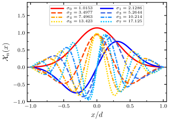
Figure 1: Function $\mathcal{X}_{n}(x):=\exp(-\beta kx^{2}/4)Y_{n}(x)/\mathcal{N}_{n}$ plotted for $n=0,1,\ldots,7$ with $\beta kd^{2}=10$. Absorbing boundary conditions are imposed in $x=\pm d$ which leads to the reported values of $\sigma_{n}$ (obtained from numerical calculations).

The explicit expression of the eigenfunctions reads

$$\psi_{n,s}(\bm{\mathrm{r}}, \vartheta)=e^{is\vartheta}\dfrac{e^{-\beta kx^{2}/4}Y_{n}(x)}{\mathcal{N}_{n}}$$ (26)

where the normalization constant has been chosen such that

$$\innerproduct{\psi_{n^{\prime},s^{\prime}}}{\psi_{n,s}}=\delta_{n,n^{\prime}}\,\delta_{s,s^{\prime}}\;.$$ (27)

Here we introduced the Kubo scalar product

$$\innerproduct{\phi}{\psi}:=\int_{-d}^{d}\!\mathrm{d}x\int_{0}^{2\pi}\!\mathrm{d}\vartheta\,p(x)\phi(x,\vartheta)^{*}\psi(x,\vartheta)\;,$$ (28)

and resorted on the fact that the functions $Y_{n}(x)$ are orthogonal and normalizable with

$$\int_{-d}^{d}\!\!\mathrm{d}x\,Y_{n}^{2}(x)=\mathcal{N}_{n}^{2}\;.$$ (29)

The isomorphism between $\ket{\psi}$ and $\psi(x,\vartheta)$ is made explicit by introducing generalized position and orientation states $|x\vartheta\rangle$ such that $\psi(x,\vartheta)=\langle x\vartheta|\psi\rangle$. Using the orthogonality condition (27) it is easy to see that the operators $\ket{\psi_{n,s}}\bra{\psi_{n,s}}$ are a set of orthogonal projectors and thus we can write the following identity relation

$$\sum_{n,s}\ket{\psi_{n,s}}\bra{\psi_{n,s}}=\mathbb{1}\;,$$ (30)

where we introduced a compact notation for the summation

$$\sum_{n,s}:=\sum_{n=0}^{\infty}\sum_{s=-\infty}^{\infty}\;.$$ (31)

The eigenfunctions of the equilibrium reference system fulfill the completeness relation

$$p(x)\!\sum_{n,s}\!\psi_{n,s}(x,\vartheta)\psi_{n,s}(x_{0},\vartheta_{0})^{*}\!=\!\delta(x\!-\!x_{0})\delta(\vartheta\!-\!\vartheta_{0})\;.$$ (32)

The previous completeness relation (32) allows us to find a solution for the reduced propagator in the equilibrium reference system starting from its formal expression (6)

$$\mathbb{P}^{(0)} (x,\vartheta,t|x_{0},\vartheta_{0})=e^{\Omega t}\delta(x-x_{0})\delta(\vartheta-\vartheta_{0})$$

$$=p(x)\sum_{n,s}\!\left\{e^{\mathcal{L}_{0}t}\psi_{n,s}(x,\vartheta)\right\}\psi_{n,s}(x_{0},\vartheta_{0})^{*}$$

$$=p(x)\sum_{n,s}\bra{x\vartheta}e^{\mathcal{L}_{0}t}\ket{\psi_{n,s}}\innerproduct{\psi_{n,s}}{x_{0}\vartheta_{0}}$$

$$=p(x)\sum_{n,s}e^{-\lambda_{n,s}t}\,\psi_{n,s}(x_{0},\vartheta_{0})^{*}\,\psi_{n,s}(x,\vartheta)\;.$$ (33)

Note that, from the second line of the previous equation and using the identity relation (30), one can also write

$$\mathbb{P}^{(0)} (x,\vartheta,t|x_{0},\vartheta_{0})=p(x)\bra{x\vartheta}e^{\mathcal{L}_{0}t}\ket{x_{0}\vartheta_{0}}\;,$$ (34)

meaning that the propagator is the projection of the generalized position and orientation state $\ket{x\vartheta}$ over the time evolution of the initial state $\ket{x_{0}\vartheta_{0}}$, multiplied by the Boltzmann weight $p(x)$.

Solution for ABP particles

One readily shows that the equilibrium operator $\mathcal{L}_{0}$ is Hermitian, $\innerproduct{\phi}{\mathcal{L}_{0}\psi}=\innerproduct{\mathcal{L}_{0}\phi}{\psi}$, with respect to the Kubo scalar product (28) and consequently its eigenvalues $\lambda_{n,s}$ are real and left and right eigenfunctions coincide, $\ket{\psi_{n,s}^{\text{L}}}=\ket{\psi_{n,s}^{\text{R}}}=\ket{\psi_{n,s}}$. However, the operator $\mathcal{L}$, taking also care of the particle’s activity, does not reflect this property. Correspondingly, in the following one has to be careful that the eigenvalues of the $\mathcal{L}$ operator, $\lambda_{n,s}^{\text{Pe}}$ are in general complex and the left eigenfunctions, $\ket{\psi_{n,s}^{\text{Pe},\text{L}}}$, are distinct from the right ones $\ket{\psi_{n,s}^{\text{Pe},\text{R}}}$. If properly normalized, the perturbed left and right eigenfunctions constitute a bi-orthonormal basis with identity relation

$$\sum_{n,s}\ket{\psi_{n,s}^{\text{Pe},\text{R}}}\bra{\psi_{n,s}^{\text{Pe},\text{L}}}=\mathbb{1}\;,$$ (35)

which directly yields the propagator in the presence of activity

$$\mathbb{P} (x,\vartheta,t|x_{0},\vartheta_{0})=\bra{x\vartheta}e^{\Omega t}\ket{x_{0}\vartheta_{0}}$$

$$=p(x)\sum_{n,s}\bra{x\vartheta}e^{\mathcal{L}t}\ket{\psi_{n,s}^{\text{Pe},\text{R}}}\innerproduct{\psi_{n,s}^{\text{Pe},\text{L}}}{x_{0}\vartheta_{0}}$$

$$=p(x)\sum_{n,s}e^{-\lambda_{n,s}^{\text{Pe}}t}\,\psi_{n,s}^{\text{Pe},\text{L}}(x_{0},\vartheta_{0})^{*}\,\psi_{n,s}^{\text{Pe},\text{R}}(x,\vartheta)\;.$$ (36)

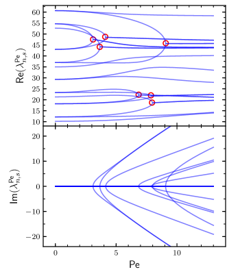
Figure 2: Numerical eigenvalues $\lambda_{n,s}$ of the Fokker-Planck operator $\mathcal{L}=\mathcal{L}_{0}+\text{Pe}\,\mathcal{L}_{1}$ as a function of the Péclet number Pe, for $\beta kd^{2}=10$, $\gamma=2$, $n_{\text{max}}=3$, and $s_{\text{max}}=2$. Transparency of lines and exceptional points highlighted with red circles better show when real components merge and imaginary ones bifurcate.

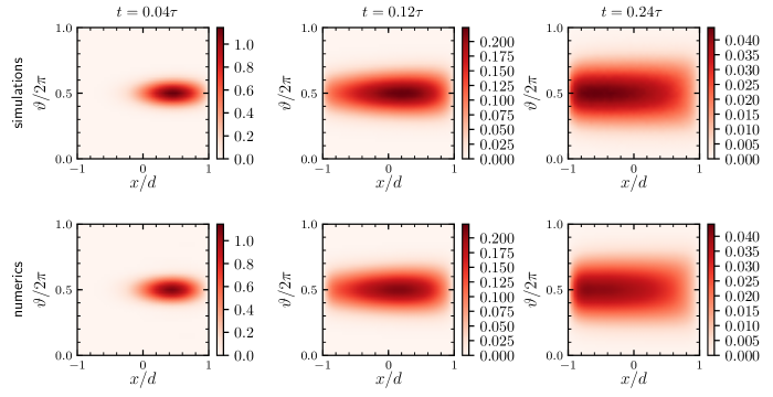
Figure 3: Probability distribution at different times $t$ starting with initial condition $x_{0}=d/2$ and $\vartheta_{0}=\pi$. Comparison between simulations, numerics for $\beta kd^{2}=10$, $\text{Pe}=6$ and $\gamma=2$. For the simulations, statistics has been collected from $10^{8}$ independent particles. For the numerics, $n_{\text{max}}=7$ and $s_{\text{max}}=6$.

To explicitly compute the propagator (Solution for ABP particles), it is then necessary to calculate the perturbed eigenvalues and left and right eigenfunction. To this scope, one has first to explicitly evaluate the action of the perturbation $\mathcal{L}_{1}$ on the eigenstates of $\mathcal{L}_{0}$. Starting from Eqs. (15) and (26) is it possible to show that

$$\mathcal{L}_{1} \ket{\psi_{n,s}}\!=\!-\dfrac{d}{2\tau}\sum_{n^{\prime}=0}^{\infty}b_{n,n^{\prime}}\big{(}\ket{\psi_{n^{\prime},s+1}}+\ket{\psi_{n^{\prime},s-1}}\big{)}$$ (37)

with weights $b_{n,n^{\prime}}$ having a rather lengthy formula which can be found in appendix A.

Now, given the finite-dimensional subspace of equilibrium eigenfunctions such that $0\leq n\leq n_{\text{max}}$ and $|s|\leq s_{\text{max}}$, the action of the full operator $\mathcal{L}=\mathcal{L}_{0}+\text{Pe}\,\mathcal{L}_{1}$ is completely characterized by a square matrix $\mathcal{G}$ of dimension $(1+n_{\text{max}})(2s_{\text{max}}+1)$ with elements defined by

$$[\mathcal{G}]_{n^{\prime}(2s_{\rm max}+1)+s^{\prime}+s_{\rm max},n(2s_{\rm max}+1)+s+s_{\rm max}}$$

$$\qquad\qquad=\bra{\psi_{n^{\prime},s^{\prime}}}\mathcal{L}_{0}+\text{Pe}\,\mathcal{L}_{1}\ket{\psi_{n,s}}\,,$$ (38)

which has to be diagonalized numerically to obtain its eigenvalues $\lambda_{n,s}^{\text{Pe}}$ and left and right eigenvectors, $\bra{\psi_{n,s}^{\text{Pe},\text{L}}}$ and $\ket{\psi_{n,s}^{\text{Pe},\text{R}}}$ for any arbitrary Péclet number. The perturbed eigenvectors are then a linear combination of the equilibrium eigenstates

$$\ket{\psi_{n,s}^{\text{Pe},\text{R}}} =\sum_{n^{\prime},s^{\prime}}g_{n,s}^{\text{R};\,n^{\prime},s^{\prime}}\ket{\psi_{n^{\prime},s^{\prime}}}\;,$$ (39)

$$\bra{\psi_{n,s}^{\text{Pe},\text{L}}} =\sum_{n^{\prime},s^{\prime}}g_{n,s}^{\text{L};\,n^{\prime},s^{\prime}}\bra{\psi_{n^{\prime},s^{\prime}}}\;.$$ (40)

The computational effort required to diagonalize such matrices increases rapidly with their dimension. However, the decaying exponentials in time in the expression of the propagator, Eq. (Solution for ABP particles), ensures convergence. In the unperturbed case, $\text{Pe}=0$, the eigenvalues (19) are real and an increasing function of $n$ and $|s|$. However, with increasing Péclet number, the real components of two distinct eigenvalues may merge and they bifurcate to a pair of complex conjugates for even larger activity, see Fig. 2. These branching points, called exceptional points Heiss (2012), often originate in parameter-dependent eigenvalue problems and occur in a great variety of physical problems including mechanics, electromagnetism, atomic and molecular physics, quantum phase transitions, and quantum chaos. They have also been observed in other problems concerning active particles Kurzthaler et al. (2016); Kurzthaler and Franosch (2017); Di Trapani et al. (2023). The exceptional point are highlighted with red circles in the upper panel of Fig. 2.

To corroborate our findings, we benchmark the time evolution of the probability distribution starting from some given initial condition as obtained from numerics against that obtained by direct stochastic simulations, see Fig. 3. Note that due to the presence of the absorbing boundary, the discretization time step adopted in the stochastic simulations should be smaller than what is usually adopted for standard simulations of an ABP in free space. As a matter of facts, with increasing time, convergence of results in the proximity of the boundary becomes more and more sensitive to the value of the discretization time step, see also appendix B in Ref. (Di Trapani et al., 2023).

Transition-Path Times Statistics

Here, we define transition paths as those trajectories originating at a given point $(x_{0}=-d+\varepsilon,y_{0})$ arbitrarily close to the left boundary ($x=-d$) and being absorbed at any point $(x=d,y)$ on the right boundary in the limit of vanishing $\varepsilon$.

The continuity equation $\partial_{t}\mathbb{P}=-\bm{\mathrm{\nabla}}\cdot\bm{\mathrm{j}}$ not allows us to write particle current in the $x$ direction associated to the Fokker–Planck equation

$$j_{x}(x,\!\vartheta|x_{0},\!\vartheta_{0})\!=\!\dfrac{d^{2}}{\tau}\left[\beta kx\!-\!\partial_{x}\!+\!\dfrac{\text{Pe}}{d}\cos\vartheta\right]\mathbb{P}(x,\!\vartheta|x_{0},\!\vartheta_{0})\,.$$ (41)

Inserting Eqs. (Solution for ABP particles), (9), (39), and (40) into Eq. (41) we get

$$j_{x} (x,\!\vartheta|x_{0},\!\vartheta_{0})=\dfrac{d^{2}}{\tau}p(x)\!\sum_{n,s}\!e^{-\lambda_{n,s}^{\text{Pe}}t}\!\sum_{n^{\prime},s^{\prime}}\!g_{n,s}^{\text{L};\,n^{\prime},s^{\prime}}\!\psi_{n^{\prime},s^{\prime}}(x_{0},\vartheta_{0})^{*}$$

$$\times\!\!\!\sum_{n^{\prime\prime},s^{\prime\prime}}\!g_{n,s}^{\text{R};\,n^{\prime\prime},s^{\prime\prime}}\left(\dfrac{\text{Pe}}{d}\cos\vartheta-\partial_{x}\right)\psi_{n^{\prime\prime},s^{\prime\prime}}(x,\vartheta)\ .$$ (42)

The TPT distribution, dependent on the initial angle $\vartheta_{0}$, is then given by Hummer (2004); Caraglio et al. (2018)

$$\quad P_{\rm TPT}(t|\vartheta_{0})=\lim_{\varepsilon\to 0}\dfrac{\int_{0}^{2\pi}\!\mathrm{d}\vartheta\,j_{x}(d,\vartheta,t|-d+\varepsilon,\vartheta_{0})}{\int_{0}^{\infty}\!\!\mathrm{d}t^{\prime}\int_{0}^{2\pi}\!\mathrm{d}\vartheta\,j_{x}(d,\vartheta,t^{\prime}|-d+\varepsilon,\vartheta_{0})}\,.$$ (43)

Recalling that the boundary condition imposes $\psi(\pm d,\vartheta)=0$, we have that

$$\psi(-d+\varepsilon,\vartheta)\approx\varepsilon\partial_{x}\psi(-d,\vartheta)\,,$$ (44)

and that the current at the $x=d$ boundary appearing in Eq. (43) does not show an explicit dependence on the Péclet number. Note, however, that such a current is still inderectly depending on the activity since the $g^{\rm L}$’s and $g^{\rm R}$’s coefficients change when vaying the Péclet number. We can thus write

$$j_{x}(d,\vartheta,t|-d+\varepsilon,\vartheta_{0})\approx-\varepsilon\dfrac{d^{2}}{\tau}p(d)\sum_{n,s}e^{-\lambda_{n,s}^{\text{Pe}}t}$$

$$\quad\times\!\sum_{n^{\prime},s^{\prime}}g_{n,s}^{\text{L};\,n^{\prime},s^{\prime}}\,\partial_{x}\,\psi_{n^{\prime},s^{\prime}}(-d,\vartheta_{0})^{*}$$

$$\quad\times\!\sum_{n^{\prime\prime},s^{\prime\prime}}g_{n,s}^{\text{R};\,n^{\prime\prime},s^{\prime\prime}}\partial_{x}\psi_{n^{\prime\prime},s^{\prime\prime}}(d,\vartheta)\ .$$ (45)

This current is of order $\varepsilon$, however this factor is canceled by using the normalization constant in Eq. (43), and hence the TPT distribution in the limit $\varepsilon\rightarrow 0$ remains finite. Integrating also over $\vartheta$,one finally obtains

$$\quad P_{\rm TPT}(t|\vartheta_{0})=\dfrac{\displaystyle\sum_{n,s}e^{-\lambda_{n,s}^{\text{Pe}}t}G^{\text{L}}_{n,s}(-d,\vartheta_{0})\,G^{\text{R}}_{n,s}(d)}{\displaystyle\sum_{n,s}\dfrac{1}{\lambda_{n,s}^{\text{Pe}}}G^{\text{L}}_{n,s}(-d,\vartheta_{0})\,G^{\text{R}}_{n,s}(d)}\,,$$ (46)

with

$$G^{\text{L}}_{n,s}(x,\vartheta):=\sum_{n^{\prime},s^{\prime}}g_{n,s}^{\text{L};\,n^{\prime},s^{\prime}}e^{-is^{\prime}\vartheta}\partial_{x}\mathcal{X}_{n^{\prime}}(x)\,,$$ (47)

and

$$G^{\text{R}}_{n,s}(x):=\sum_{n^{\prime}}g_{n,s}^{\text{R};\,n^{\prime},0}\,\partial_{x}\mathcal{X}_{n^{\prime}}(x)\,,$$ (48)

with $\mathcal{X}_{n}(x):=\exp(-\beta kx^{2}/4)Y_{n}(x)/\mathcal{N}_{n}$. In the limit of vanishing activity ($\text{Pe}=0$) one recovers the TPT distribution of a one-dimensional passive particle crossing a parabolic barrier as reported in Ref. Caraglio et al. (2018).

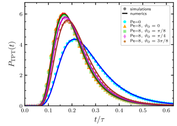
Figure 4: Transition-path-time distribution, $P_{\rm TPT}(t)=P_{\rm TPT}(t|\vartheta_{0})$, as a function of the direction of the self-propulsion at the left boundary, $\vartheta_{0}=0$. Comparison between simulations (symbols) and numerics (lines) for $\beta kd^{2}=10$ and $\gamma=2$ For the simulations, statistics has been collected from $10^{6}$ independent transition paths defined as paths starting at $x=-d+\varepsilon$ with $\varepsilon=10^{-7}$ and ending at $x=d$. For the numerics, $n_{\rm max}=32$ and $s_{\rm max}=6$.

Our results show that the peak of the TPT distribution of an active particle for a relatively high barrier ($\beta kd^{2}=10$) is shifted to the left with respect to the peak of the TPT distribution of a passive particle, see Fig. 4. Surprisingly, the TPT distribution depends only mildly on the initial direction of the self-propulsion when starting from the left boundary ($x=-d$). Furthermore, we also note that the average TPT decreases with the activity of the particle. Interestingly, this result aligns with what is observed in one-dimensional systems Carlon et al. (2018) while the opposite behavior is observed in different two-dimensional systems Zanovello et al. (2021a, b).

Survival probability and first-passage-time distribution

The knowledge of the reduced propagator allows to compute also the survival probability at time $t$. The latter, given some initial conditions $(x_{0},\vartheta_{0})$, is readily obtained by integrating over the final $x$ coordinate and orientation

$$S(t|x_{0},\vartheta_{0})\!=\!\int_{-d}^{d}\!\!\mathrm{d}x\int_{0}^{2\pi}\!\!\!\!\mathrm{d}\vartheta\,\mathbb{P}(x,\vartheta,t|x_{0},\vartheta_{0})\;.$$ (49)

Since

$$\int_{-d}^{d}\!\!\mathrm{d}x\int_{0}^{2\pi}\!\!\!\!\mathrm{d}\vartheta\,p(x)\psi_{n,s}(x,\vartheta)=\delta_{s,0}\,f_{n}\;,$$ (50)

with

$$f_{n}\!:=\!\left\{\!\!\!\begin{array}[]{l}\dfrac{1}{\mathcal{N}_{n}}\displaystyle\!\int_{-d}^{d}\!\!\!\mathrm{d}x\;{{}_{1}\!}F_{1}\!\!\left(\dfrac{1}{2}\!-\!\dfrac{\sigma_{n}}{2}\!;\dfrac{1}{2}\!;\dfrac{\beta kx^{2}}{2}\right)\mbox{ if }n=0,2,\ldots\\ \\ 0\qquad\qquad\mbox{else}\,,\end{array}\right.$$ (54)

exploiting Eqs. (Solution for ABP particles), (39), and (40), one obtains

$$S (t|x_{0},\vartheta_{0})=\sum_{n,s}e^{-\lambda_{n,s}^{\text{Pe}}t}$$

$$\times\!\!\!\sum_{n^{\prime},s^{\prime}}g_{n,s}^{\text{L};\,n^{\prime},s^{\prime}}\psi_{n^{\prime},s^{\prime}}(x_{0},\vartheta_{0})^{*}\sum_{n^{\prime\prime}}g_{n,s}^{\text{R};\,n^{\prime\prime},0}f_{n^{\prime\prime}}\,.$$ (55)

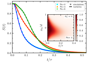
Figure 5: Survival probability, $S(t)=S(t|x_{0},\vartheta_{0})$, as a function of time for different Pe and with initial condition $x_{0}=-d/2$ and $\vartheta_{0}=0$. Comparison between simulations (symbols) and numerics (lines) for $\beta kd^{2}=10$ and $\gamma=0.4$ For the simulations, statistics has been collected from $10^{5}$ independent particles. For the numerics, $n_{\rm max}=12$ and $s_{\rm max}=6$. Inset: Survival probability as a function of time and $x_{0}$ for $\text{Pe}=4$ as obtained from numerics for the remaining initial condition $\vartheta_{0}=0$.

See Fig. 5 for a comparison between the results at different Péclet numbers obtained by numerics and by direct stochastic simulations. As expected, due to their activity and the persistence of their motion, active particles display a different behavior with respect to standard passive Brownian particles. For example, starting with an initial position at $x_{0}=-d/2$ we can note that a passive particle has a $50\%$ probability of being absorbed at the boundaries within a time of about $0.06\tau$, see Fig. 5. This quick initial decay of the survival probability is due to the fact that the passive particle is likely unable to overcome the potential barrier and is soon absorbed at the left boundary of the box ($x=0$). On the other hand, with increasing activity and initial direction pointing towards the barrier ($\vartheta_{0}=0$), an ABP particle has more and more chances of crossing the barrier which results in an initially slower decay of the survival probability. However, once the active particle reaches the peak of the energy potential, the self-propulsion starts enhancing the probability of being absorbed at longer times. Consequently, the survival probability decreases faster at longer times with increasing activity, see Fig. 5.

Furthermore, starting from Eq. (49) we can also obtain the first-passage-time distribution for any given initial condition as

$$F(t|x_{0},\vartheta_{0})=-\dfrac{\mathrm{d}S(t|x_{0},\vartheta_{0})}{\mathrm{d}t}\;.$$ (56)

As for the survival probability, the ABP exhibits first-passage properties that differ from those of a passive particle. In particular, again starting with the initial state ($x_{0}=-d/2$, $\vartheta_{0}=0$), the first-passage-time distribution at large Péclet numbers shows a bump at short times and a faster decay at longer times, see Fig. 6. One can also note that, at least for the considered initial conditions and parameters, the rotational diffusivity influences the shape of distribution only to a limited extent, see Fig. 6.

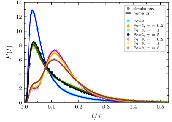
Figure 6: First-passage-time distribution, $F(t)=F(t|x_{0},\vartheta_{0})$ for different Pe and $\gamma$ and with initial condition $x_{0}=-d/2$ and $\vartheta_{0}=0$. Comparison between simulations (symbols) and numerics (lines) for $\beta kd^{2}=10$. For the simulations, statistics has been collected from $10^{7}$ independent particles. For the numerics, $n_{\rm max}=60$ and $s_{\rm max}=5$.

Note that to reach convergence in the first-passage-time distribution a much larger value of $n_{\rm max}$ is needed in comparison to that used to obtain the survival probability or the probability distribution. This observation is due to the fact that, when taking the time derivative of the survival probability, a factor equal to the eigenvalue $\lambda_{n,s}^{\text{Pe}}$ appears in the series expansion of the first-passage-time distribution. Thus, while already for the survival probability it is necessary to consider more and more terms in the summation (Survival probability and first-passage-time distribution) when time decreases, this issue becomes even more important for the first-passage-time distribution.

Conclusions

We have derived an exact series solution for the probability propagator (along the $x$ coordinate and the self-propulsion angle) of a two-dimensional ABP living in a domain with absorbing boundaries at $x=\pm d$ and subjected to a parabolic potential along the $x$ direction, centered at $x=0$. Such a solution is possible by taking the standard passive Brownian motion as a reference system and dealing with the activity of the particle as a perturbation. The reduced propagator is then expressed in terms of the left and right eigenvectors, which can be easily computed by direct diagonalization of the matrix form of the Fokker-Planck operator, multiplied by an exponentially decaying factor with a rate given by the corresponding perturbed eigenvalue. The approach adopted in this work takes inspiration from the one recently adopted to solve the ABP model in a circular harmonic trap Caraglio and Franosch (2022). However, in contrast to what happens in the case of an isotropic harmonic potential, in the present case switching on the particle activity induces a change in the eigenvalue spectrum of the Fokker-Planck operator. With increasing activity more and more eigenvalues become complex and exceptional points Heiss (2012) arise.

The knowledge of the propagator is then exploited as a starting point to obtain several observables. In particular, given some initial condition, we compute the spatial probability density at a later time (integration of the propagator over the self-propulsion orientation $\vartheta$), the survival probability (integration over all coordinates), and the related first-passage-time distribution. All these quantities show a strong dependence on the activity of the particle and, to a lesser extent, on its rotational diffusivity. This observation is in line with what observed for and ABP exploring a circular domain with an absorbing boundary Di Trapani et al. (2023). We also derive the distribution of the transition-path time, i.e. of the time needed to travel from the boundary on one side of the barrier to the boundary on the other side.

Besides extending the nowadays limited set of exactly solvable models for active particles Wagner et al. (2017); Hermann and Schmidt (2018); Schnitzer (1993); Tailleur and Cates (2008, 2009); Malakar et al. (2018); Kurzthaler et al. (2016); Kurzthaler and Franosch (2017); Kurzthaler et al. (2018); Martens et al. (2012); Sevilla and Sandoval (2015); Caraglio and Franosch (2022); Di Trapani et al. (2023), our findings also pile on the recent literature regarding first-passage properties of active particles Malakar et al. (2018); Angelani et al. (2014); Scacchi and Sharma (2018); Demaerel and Maes (2018); Dhar et al. (2019); Basu et al. (2018) and can be exploited to reach analytical insight into target-search Tejedor et al. (2012); Volpe and Volpe (2017); Zanovello et al. (2021a, b) problems in more complex environments involving absorbing boundaries. Furthermore, to the best of our knowledge, analytical expressions for TPT distribution in the case of active forces have been previously obtained only in the case of one-dimensional systems Carlon et al. (2018). Thus, our derivation of the TPT distribution in the presence of absorbing boundaries for a two-dimensional active particle represents a significative advance in the field.

Appendix A Action of $\mathcal{L}_{1}$ on the equilibrium eigenfunction $\ket{\psi_{n,s}}$

Here, we now explicitly evaluate the action of the perturbation $\mathcal{L}_{1}$ on the eigenstates of $\mathcal{L}_{0}$ obtained from the eigenvalue problem

$$\mathcal{L}_{0}\psi_{n,s}(\bm{\mathrm{r}},\vartheta)=-\lambda_{n,s}\ket{\psi_{n,s}}\;.$$ (57)

Considering Eqs. (15) and (26) we have

$$\mathcal{L}_{1} \ket{\psi_{n,s}}=-\dfrac{d}{\tau}\Bigg{\{}\left(\dfrac{e^{i(s+1)\vartheta}+e^{i(s-1)\vartheta}}{2}\right)(\beta kx+\partial_{x})\dfrac{e^{-\beta kx^{2}/4}Y_{n}(x)}{\mathcal{N}_{n}}\Bigg{\}}\;,$$ (58)

and

$$(\beta kx+\partial_{x})\dfrac{e^{-\beta kx^{2}/4}Y_{n}(x)}{\mathcal{N}_{n}}=\left\{\begin{array}[]{ll}\dfrac{\beta k(1\!-\!\sigma_{n})}{\mathcal{N}_{n}}xe^{-\beta kx^{2}/2}{{}_{1}\!}F_{1}\!\left(\dfrac{3}{2}\!-\!\dfrac{\sigma_{n}}{2};\dfrac{3}{2};\dfrac{\beta kx^{2}}{2}\right)&\quad n\!=\!0,2,4,\ldots\\ &\\ \dfrac{1}{\mathcal{N}_{n}}\sqrt{\beta k}e^{-\beta kx^{2}/2}\,{{}_{1}\!}F_{1}\!\left(\!1\!-\!\dfrac{\sigma_{n}}{2};\dfrac{3}{2};\dfrac{\beta kx^{2}}{2}\!\right)&\\ \quad+\dfrac{2-\sigma_{n}}{3\mathcal{N}_{n}}(\beta k)^{3/2}x^{2}e^{-\beta kx^{2}/2}{{}_{1}\!}F_{1}\!\left(2\!-\!\dfrac{\sigma_{n}}{2};\dfrac{5}{2};\dfrac{\beta kx^{2}}{2}\right)&\quad n\!=\!1,3,\ldots\end{array}\right.$$ (63)

where we used the property DLMF

$$\partial_{z}\;{{}_{1}\!}F_{1}(a;b;z)=\dfrac{a}{b}\;{{}_{1}\!}F_{1}(a+1;b+1;z)$$ (64)

These function are odd for $n=0,2,4,\ldots$ and even for $n=1,3,\ldots$.

We note then that given a complete orthogonal system of functions $\{\phi_{\ell}(z)\}$ over the interval $\mathcal{R}$, the functions $\phi_{\ell}(z)$ satisfy an orthogonality relationship of the form

$$\int_{\mathcal{R}}\mathrm{d}z\,w(z)\phi_{\ell^{\prime}}(z)\phi_{\ell}(z)=c_{\ell}\delta_{\ell,\ell^{\prime}}\;,$$ (65)

where $w(z)$ is a a weighting function, $c_{\ell}$ are given constants and $\delta_{\ell,\ell^{\prime}}$ is the Kronecker delta. An arbitrary function $f(z)$ can be written as a series

$$f(z)=\sum_{\ell=0}^{\infty}a_{\ell}\phi_{\ell}(z)\;,$$ (66)

with

$$a_{\ell}=\dfrac{1}{c_{\ell}}\int_{\mathcal{R}}\mathrm{d}z\,w(z)\phi_{\ell}(z)f(z)\;.$$ (67)

Substituting $z$ with $x$ and applying relations (65)-(67) to the case in which $\phi_{n}(x)=e^{-\beta kx^{2}/4}Y_{n}(x)/\mathcal{N}_{n}$, $f(x)$ is given by Eq. (63), $w(x)=e^{\beta kx^{2}/2}$, and $c_{n}=1$ we have

$$\quad(\beta kx+\partial_{x})\dfrac{e^{-\beta kx^{2}/4}Y_{n}(x)}{\mathcal{N}_{n}}=\!\sum_{n^{\prime}=0}^{\infty}b_{n,n^{\prime}}\dfrac{e^{-\beta kx^{2}/4}Y_{n^{\prime}}(x)}{\mathcal{N}_{n^{\prime}}}\;,$$ (68)

with

$$b_{n,n^{\prime}}=\left\{\begin{array}[]{ll}\dfrac{\beta k(1\!-\!\sigma_{n})}{\mathcal{N}_{n}\mathcal{N}_{n^{\prime}}}\displaystyle\int_{-d}^{d}\mathrm{d}x\,e^{-\beta kx^{2}/4}Y_{n^{\prime}}(x)\,x\,{{}_{1}\!}F_{1}\!\left(\dfrac{3}{2}\!-\!\dfrac{\sigma_{n}}{2};\dfrac{3}{2};\dfrac{\beta kx^{2}}{2}\right)&\mbox{ if }n=0,2,\ldots\mbox{ and }n^{\prime}=1,3,\ldots\\ &\\ \dfrac{\sqrt{\beta k}}{\mathcal{N}_{n}\mathcal{N}_{n^{\prime}}}\displaystyle\int_{-d}^{d}\mathrm{d}x\,e^{-\beta kx^{2}/4}Y_{n^{\prime}}(x)\Bigg{[}{{}_{1}\!}F_{1}\!\left(\!1\!-\!\dfrac{\sigma_{n}}{2};\dfrac{3}{2};\dfrac{\beta kx^{2}}{2}\!\right)&\\ \quad+\dfrac{2-\sigma_{n}}{3}\beta kx^{2}{{}_{1}\!}F_{1}\!\left(2\!-\!\dfrac{\sigma_{n}}{2};\dfrac{5}{2};\dfrac{\beta kx^{2}}{2}\right)\Bigg{]}&\mbox{ if }n=1,3,\ldots\mbox{ and }n^{\prime}=0,2,\ldots\\ &\\ 0&\mbox{ otherwise}\\ \end{array}\right.$$ (75)

Finally, inserting the above relations into Eq. (58) one gets

$$\mathcal{L}_{1} \ket{\psi_{n,s}}=-\dfrac{d}{2\tau}\sum_{n^{\prime}=0}^{\infty}b_{n,n^{\prime}}\big{(}\ket{\psi_{n^{\prime},s+1}}+\ket{\psi_{n^{\prime},s-1}}\big{)}$$ (76)

References

- Bechinger et al. (2016) C. Bechinger, R. Di Leonardo, H. Löwen, C. Reichhardt, G. Volpe, and G. Volpe, “Active particles in complex and crowded environments,” Rev. Mod. Phys. 88, 045006 (2016).
- Marchetti et al. (2013) M. C. Marchetti, J. F. Joanny, S. Ramaswamy, T. B. Liverpool, J. Prost, M. Rao, and R. A. Simha, “Hydrodynamics of soft active matter,” Rev. Mod. Phys. 85, 1143 (2013).
- Romanczuk et al. (2012) P. Romanczuk, M. Bär, W. Ebeling, B. Lindner, and L. Schimansky-Geier, “Active Brownian particles,” Eur. Phys. J.: Spec. Top. 202, 1 (2012).
- Elgeti et al. (2015) J. Elgeti, R. Winkler, and G. G., “Physics of microswimmers – single particle motion and collective behavior: a review,” Rep. Prog. Phys. 78, 056601 (2015).
- Needleman and Dogic (2017) D. Needleman and Z. Dogic, “Active matter at the interface between materials science and cell biology,” Nat. Rev. Mater. 2, 17048 (2017).
- Lipowsky and Klumpp (2005) R. Lipowsky and S. Klumpp, “Life is motion: multiscale motility of molecular motors,” Phys. A (Amsterdam, Neth.) 352, 53 (2005).
- Wang and Gao (2012) J. Wang and W. Gao, “Nano/microscale motors: Biomedical opportunities and challenges,” ACS Nano 6, 5745 (2012).
- Henkes et al. (2020) S. Henkes, K. Kostanjevec, J. M. Collinson, R. Sknepnek, and E. Bertin, “Dense active matter model of motion patterns in confluent cell monolayers,” Nat. Commun. 11, 1405 (2020).
- Cheang et al. (2014) K. U. Cheang, L. Kyoungwoo, J. Anak Agung, and K. Min Jun, “Multiple-robot drug delivery strategy through coordinated teams of microswimmers,” Appl. Phys. Lett. 105, 083705 (2014).
- Erkoc et al. (2019) P. Erkoc, I. C. Yasa, H. Ceylan, O. Yasa, Y. Alapan, and M. Sitti, “Mobile microrobots for active therapeutic delivery,” Adv. Ther. (Weinheim, Ger.) 2, 1800064 (2019).
- Helbing (2001) D. Helbing, “Traffic and related self-driven many-particle systems,” Rev. Mod. Phys. 73, 1067 (2001).
- Cates (2012) M. E. Cates, “Diffusive transport without detailed balance in motile bacteria: Does microbiology need statistical physics?” Rep. Prog. Phys. 75, 042601 (2012).
- Chaudhuri (2014) D. Chaudhuri, “Active Brownian particles: Entropy production and fluctuation response,” Phys. Rev. E 90, 022131 (2014).
- Fodor et al. (2016) É. Fodor, C. Nardini, M. E. Cates, J. Tailleur, P. Visco, and F. van Wijland, “How far from equilibrium is active matter?” Phys. Rev. Lett. 117, 038103 (2016).
- Falasco et al. (2016) G. Falasco, R. Pfaller, A. P. Bregulla, F. Cichos, and K. Kroy, “Exact symmetries in the velocity fluctuations of a hot Brownian swimmer,” Phys. Rev. E 94, 030602(R) (2016).
- Speck (2016) T. Speck, “Stochastic thermodynamics for active matter,” Europhys. Lett. 114, 30006 (2016).
- Fodor and Marchetti (2018) É. Fodor and M. C. Marchetti, “The statistical physics of active matter: From self-catalytic colloids to living cells,” Phys. A (Amsterdam, Neth.) 504, 106 (2018).
- Caraglio and Franosch (2022) M. Caraglio and T. Franosch, “Analytic solution of an active brownian particle in a harmonic well,” Phys. Rev. Lett. 129, 158001 (2022).
- Kumar et al. (2014) N. Kumar, H. Soni, S. Ramaswamy, and A. K. Sood, “Flocking at a distance in active granular matter,” Nat. Commun. 5, 4688 (2014).
- Fily and Marchetti (2012) Y. Fily and M. C. Marchetti, “Athermal phase separation of self-propelled particles with no alignment,” Phys. Rev. Lett. 108, 235702 (2012).
- Slowman et al. (2016) A. B. Slowman, M. R. Evans, and R. A. Blythe, “Jamming and attraction of interacting run-and-tumble random walkers,” Phys. Rev. Lett. 116, 218101 (2016).
- Stenhammar et al. (2015) J. Stenhammar, R. Wittkowski, D. Marenduzzo, and M. E. Cates, “Activity-induced phase separation and self-assembly in mixtures of active and passive particles,” Phys. Rev. Lett. 114, 018301 (2015).
- Elgeti and Gompper (2013) J. Elgeti and G. Gompper, “Wall accumulation of self-propelled spheres,” Europhys. Lett. 101, 48003 (2013).
- Volpe et al. (2014) G. Volpe, S. Gigan, and G. Volpe, “Simulation of the active Brownian motion of a microswimmer,” Am. J. Phys. 82, 659 (2014).
- Tailleur and Cates (2009) J. Tailleur and M. E. Cates, “Sedimentation, trapping, and rectification of dilute bacteria,” Europhys. Lett. 86, 60002 (2009).
- Malakar et al. (2018) K. Malakar, V. Jemseena, A. Kundu, K. Kumar, S. Sabhapandit, S. Majumdar, S. Redner, and A. Dhar, “Steady state, relaxation and first-passage properties of a run-and-tumble particle in one-dimension,” J. Stat. Mech. Theory Exp. 2018, 043215 (2018).
- Wagner et al. (2017) C. G. Wagner, M. F. Hagan, and A. Baskaran, “Steady-state distributions of ideal active Brownian particles under confinement and forcing,” J. Stat. Mech. Theory Exp. 2017, 043203 (2017).
- Malakar et al. (2020) K. Malakar, A. Das, A. Kundu, K. V. Kumar, and A. Dhar, “Steady state of an active Brownian particle in a two-dimensional harmonic trap,” Phys. Rev. E 101, 022610 (2020).
- Kurzthaler et al. (2016) C. Kurzthaler, S. Leitmann, and T. Franosch, “Intermediate scattering function of an anisotropic active Brownian particle,” Sci. Rep. 6, 36702 (2016).
- Kurzthaler and Franosch (2017) C. Kurzthaler and T. Franosch, “Intermediate scattering function of an anisotropic Brownian circle swimmer,” Soft Matter 13, 6396 (2017).
- Kurzthaler et al. (2018) C. Kurzthaler, C. Devailly, J. Arlt, T. Franosch, W. C. K. Poon, V. A. Martinez, and A. T. Brown, “Probing the Spatiotemporal Dynamics of Catalytic Janus Particles with Single-Particle Tracking and Differential Dynamic Microscopy,” Phys. Rev. Lett. 121, 078001 (2018).
- Hermann and Schmidt (2018) S. Hermann and M. Schmidt, “Active ideal sedimentation: Exact two-dimensional steady states,” Soft Matter 14, 1614 (2018).
- Schnitzer (1993) M. J. Schnitzer, “Theory of continuum random walks and application to chemotaxis,” Phys. Rev. E 48, 2553 (1993).
- Tailleur and Cates (2008) J. Tailleur and M. E. Cates, “Statistical Mechanics of Interacting Run-and-Tumble Bacteria,” Phys. Rev. Lett. 100, 218103 (2008).
- Martens et al. (2012) K. Martens, L. Angelani, R. Di Leonardo, and L. Bocquet, “Probability distributions for the run-and-tumble bacterial dynamics: An analogy to the Lorentz model,” Eur. Phys. J. E 35, 84 (2012).
- Sevilla and Sandoval (2015) F. J. Sevilla and M. Sandoval, “Smoluchowski diffusion equation for active Brownian swimmers,” Phys. Rev. E 91, 052150 (2015).
- Di Trapani et al. (2023) F. Di Trapani, T. Franosch, and M. Caraglio, “Active Brownian particles in a circular disk with an absorbing boundary,” Phys. Rev. E 107, 064123 (2023).
- Caraglio et al. (2018) M. Caraglio, S. Put, E. Carlon, and C. Vanderzande, “The influence of absorbing boundary conditions on the transition path time statistics,” Phys. Chem. Chem. Phys. 20, 25676 (2018).
- Caraglio (2024) M. Caraglio, “Ttwo-dimensional active brownian particles crossing a parabolic barrier: Finite rectangular domain with absorbing boundary conditions,” xxx (2024), companion paper.
- Chung et al. (2009) H. S. Chung, J. M. Louis, and W. A. Eaton, “Experimental determination of upper bound for transition path times in protein folding from single-molecule photon-by-photon trajectories,” Proc. Natl. Acad. Sci. USA 106, 11837 (2009).
- Neupane et al. (2016) K. Neupane, D. A. N. Foster, D. R. Dee, H. Yu, F. Wang, and M. T. Woodside, “Direct observation of transition paths during the folding of proteins and nucleic acids,” Science 352, 239 (2016).
- Neupane et al. (2017) K. Neupane, F. Wang, and M. T. Woodside, “Direct measurement of sequence-dependent transition path times and conformational diffusion in DNA duplex formation,” Proc. Natl. Acad. Sci. USA 114, 1329 (2017).
- Neupane et al. (2018) K. Neupane, N. Q. Hoffer, and M. T. Woodside, “Measuring the local velocity along transition paths during the folding of single biological molecules,” Phys. Rev. Lett. 121, 018102 (2018).
- Zhang et al. (2007) B. W. Zhang, D. Jasnow, and D. M. Zuckerman, “Transition-event durations in one-dimensional activated processes,” J. Chem. Phys. 126, 074504 (2007).
- Faccioli and Pederiva (2012) P. Faccioli and F. Pederiva, “Microscopically computing free-energy profiles and transition path time of rare macromolecular transitions,” Phys. Rev. E 86, 061916 (2012).
- Kim and Netz (2015) W. K. Kim and R. R. Netz, “The mean shape of transition and first-passage paths,” J. Chem. Phys. 143, 224108 (2015).
- Makarov (2015) D. E. Makarov, “Shapes of dominant transition paths from single-molecule force spectroscopy,” J. Chem. Phys. 143, 194103 (2015).
- Laleman et al. (2017) M. Laleman, E. Carlon, and H. Orland, “Transition path time distributions,” J. Chem. Phys. 147, 214103 (2017).
- Caraglio et al. (2020) M. Caraglio, T. Sakaue, and E. Carlon, “Transition path times in asymmetric barriers,” Phys. Chem. Chem. Phys. 22, 3512 (2020).
- Redner (2001) S. Redner, A Guide to First-Passage Processes (Cambridge University Press, 2001).
- Metzler et al. (2013) R. Metzler, G. Oshanin, and S. Redner, eds., First-Passage Phenomena and Their Applications (World Scientific, Singapore, 2013).
- Risken (1989) H. Risken, The Fokker-Planck Equation (Springer, Berlin, 1989).
- Palyulin et al. (2019) V. V. Palyulin, G. Blackburn, M. A. Lomholt, N. W. Watkins, R. Metzler, R. Klages, and A. V. Chechkin, “First passage and first hitting times of Lévy flights and Lévy walks,” New J. Phys. 21, 103028 (2019).
- Gerstner et al. (1997) W. Gerstner, A. K. Kreiter, H. Markram, and A. V. M. Herz, “Neural codes: Firing rates for integral transforms in terms of whittaker functions see §13.23(ivand beyond,” Proc. Natl. Acad. Sci. USA 94, 12740 (1997).
- Sazuka et al. (2009) N. Sazuka, J.-i. Inoue, and E. Scalas, “The distribution of first-passage times and durations in FOREX and future markets,” Phys. A: Stat. Mech. Appl. 388, 2839 (2009).
- Baldovin et al. (2015) F. Baldovin, F. Camana, M. Caporin, M. Caraglio, and A. Stella, “Ensemble properties of high-frequency data and intraday trading rules,” Quant. Finance 15, 231 (2015).
- Chmeliov et al. (2013) J. Chmeliov, L. Valkunas, T. P. J. Krüger, C. Ilioaia, and R. van Grondelle, “Fluorescence blinking of single major light-harvesting complexes,” New J. Phys. 15, 085007 (2013).
- Iyer-Biswas and Zilman (2016) S. Iyer-Biswas and A. Zilman, “First-passage processes in cellular biology,” Adv. Chem. Phys. 160, 261 (2016).
- Abramowitz and Stegun (1964) M. Abramowitz and I. Stegun, Handbook of mathematical functions: with formulas, graphs, and mathematical tables (Courier Corporation, 1964).
- Sakurai (1994) J. J. Sakurai, Modern quantum mechanics (Addison-Wesley, 1994).
- Heiss (2012) W. D. Heiss, “The physics of exceptional points,” J. Phys. A Math. Theor. 45, 444016 (2012).
- (62) Note that here we abused notation by writing and , thus including in the vectorial notation a component.
- Hummer (2004) G. Hummer, “From transition paths to transition states and rate coefficients,” J. Chem. Phys. 120, 516 (2004).
- Carlon et al. (2018) E. Carlon, H. Orland, T. Sakaue, and C. Vanderzande, “Effect of memory and active forces on transition path time distributions,” J. Phys. Chem. B 122, 11186 (2018).
- Zanovello et al. (2021a) L. Zanovello, M. Caraglio, T. Franosch, and P. Faccioli, “Target search of active agents crossing high energy barriers,” Phys. Rev. Lett. 126, 018001 (2021a).
- Zanovello et al. (2021b) L. Zanovello, P. Faccioli, T. Franosch, and M. Caraglio, “Optimal navigation strategy of active Brownian particles in target-search problems,” J. Chem. Phys. 155, 084901 (2021b).
- Angelani et al. (2014) L. Angelani, R. Di Leonardo, and M. Paoluzzi, “First-passage time of run-and-tumble particles,” Eur. Phys. J. E 37, 59 (2014).
- Scacchi and Sharma (2018) A. Scacchi and A. Sharma, “Mean first passage time of active Brownian particle in one dimension,” Mol. Phys. 116, 460 (2018).
- Demaerel and Maes (2018) T. Demaerel and C. Maes, “Active processes in one dimension,” Phys. Rev. E 97, 032604 (2018).
- Dhar et al. (2019) A. Dhar, A. Kundu, S. N. Majumdar, S. Sabhapandit, and G. Schehr, “Run-and-tumble particle in one-dimensional confining potentials: Steady-state, relaxation, and first-passage properties,” Phys. Rev. E 99, 032132 (2019).
- Basu et al. (2018) U. Basu, S. N. Majumdar, A. Rosso, and G. Schehr, “Active Brownian motion in two dimensions,” Phys. Rev. E 98, 062121 (2018).
- Tejedor et al. (2012) V. Tejedor, R. Voituriez, and O. Bénichou, “Optimizing persistent random searches,” Phys. Rev. Lett. 108, 088103 (2012).
- Volpe and Volpe (2017) G. Volpe and G. Volpe, “The topography of the environment alters the optimal search strategy for active particles,” Proc. Natl. Acad. Sci. USA 114, 11350 (2017).
- (74) DLMF, “NIST Digital Library of Mathematical Functions,” F. W. J. Olver, A. B. Olde Daalhuis, D. W. Lozier, B. I. Schneider, R. F. Boisvert, C. W. Clark, B. R. Miller, B. V. Saunders, H. S. Cohl, and M. A. McClain, eds.