Topological phase transition in anti-symmetric Lotka-Volterra doublet chain
Abstract
We present the emergence of topological phase transition in the minimal model of two dimensional rock-paper-scissors cycle in the form of a doublet chain. The evolutionary dynamics of the doublet chain is obtained by solving the anti-symmetric Lotka-Volterra equation. We show that the mass decays exponentially towards edges and robust against small perturbation in the rate of change of mass transfer, a signature of a topological phase. For one of the configuration of our doublet chain, the mass is transferred towards both edges and the bulk is gaped. Further, we confirm this phase transition within the framework of topological band theory. For this we calculate the winding number which change from zero to one for trivial and a non-trivial topological phases respectively.
Introduction. Topology plays a vital role in condensed matter physics Thouless et al. (1982); Jiang et al. (2012); Haldane (1988). Topological phase transition is one of those properties that has been previously studied in the context of quantum systems, but recent works have shown this phenomenon is observed in mechanical meta-materialsKane and Lubensky (2014); Chen et al. (2016); Fan et al. (2019), active matter Sone et al. (2020), and photonic crystals Raghu and Haldane (2008); Ozawa et al. (2019); He et al. (2020). Robustness, condensation, localization and phase transitions are key characteristics of this kind of system Haldane (1988). This condensation phenomenon has also been observed in systems like citation networks Krapivsky et al. (2000); Bianconi and Barabási (2001), jamming of traffic Kaupužs et al. (2005) or mass transport modelsEvans and Waclaw (2014). As biological systems and soft matter have shown properties of topological phases Prodan and Prodan (2009); Nash et al. (2015); Souslov et al. (2017); Pedro et al. (2019); Yoshida and Hatsugai (2021), one key area of interest is how these non-trivial topological properties can be obtained in a designed biological set-up.
Recent studies have shown that anti-symmetric Lotka-Volterra Equation (ALVE) applied to a lattice or chain-like structure can essentially reproduce the properties of topological phase Knebel et al. (2020); Yoshida et al. (2022); Liang et al. (2024) or chiral edge modesYoshida et al. (2021). ALVE is a non-linear mass-preserving model of entities interacting in cycles, which has been introduced for the study of population dynamics. In a generic system of constituents, mass can be regarded as the normalized quantity of each of them. Even if the constituents are interacting with each other and their mass is being transferred, the total mass remains constant throughout the process. Interestingly, ALVE has been used in different fields like quantum physics Vorberg et al. (2013), evolutionary game theory Chawanya and Tokita (2002), population dynamics GOEL et al. (1971); May (2019), chemical kinetics Di Cera et al. (1989) and plasma physics Zakharov et al. (1974); Manakov (1975) to describe condensation processes. This provides a motivation to establish equivalence between such systems. Recently, Knebel et.al.Knebel et al. (2020) have shown how the properties of an ALVE equation applied on a one-dimensional Rock-Paper-Scissor (RPS) chain on the basis of localization and robustness, can be used to mimic the topological phase transition. Particularly, with a suitable choice of interaction, mass is transferred largely to the boundary of the chain. The result is robust with respect to the model parameter heterogeneity, and a phase transition occurs at a critical value of the parameter.
Mapping RPS systems beyond one dimensional lattices have also been exercised earlier. For example, an RPS system within the structure of Kagome lattice have shown the emergence of the chiral edge mode Yoshida et al. (2021). RPS interaction realized in 3D lattice has been reported to exhibit surface polarization of mass that can be understood from the 3D Weyl semimetal phases Umer and Gong (2022). These works have opened up avenues to understand dynamical features of one and higher dimensional nonlinear systems in the light of topological band theory which was earlier limited to linear systems only.
With similar motivation i.e. to investigate the topological aspect of the RPS system in higher dimensions, we start with a doublet chain as an extension and explore the mass transfer propagation from one node to other through ALVE dynamics. This doublet chain is constructed by periodic repetition of two merged RPS triangles via a single vertex (See Fig. 1). Keeping the interaction of the RPS chain similar to the one in Knebel et al. (2020), we found that the masses are shifted to one side of the doublet chain; a property similar to what was observed in Knebel et al. (2020). Moreover, as this structure can encompass more complexity by keeping one RPS chain as before and swapping the interaction between Paper-Scissor and Scissor-Rock, most of the masses are concentrated at the diagonal corner which has not been observed before. These results are robust in terms of parameter values and remain present for large doublet chains.
Model. The ALVE describing the mass at each site is given by a system of coupled non-linear ordinary differential equations,
| (1) |
where , and are the elements of the antisymmetric matrix . The site and its interaction with its neighbours are determined by the elements of . Particularly, is considered as the (signed) rate at which mass is transferred from the site to site . Here the whole system conserves mass at each time () Knebel et al. (2020). To start with, we have taken normalized (), random, and non-zero initial masses () in the system.
To take a step towards understanding the two dimensional system, we extended the 1-D chain proposed by Knebel et al Knebel et al. (2020) to a doublet structure as shown in Fig. 1. Here, we construct it by joining two triangle sub-units through one of the vertex and then extending it by repeating. On each triangle sub-unit, mass transfer is cyclic. For both configurations, red, blue, and green, arrows represent the strength of , , and respectively. The direction of the arrow represents the direction of mass transfer. Here we have shown two types of doublet configurations depicted in Fig. 1. We create these two configurations by switching between and in the lower triangular chain. For configurations 1 & 2, the flow of mass in the upper nodes and lower nodes are in the same direction. Hence, following the direction of the arrows, we find anti-clockwise motion in the lower triangles and clockwise motion in the upper triangle. For configuration 1, the middle nodes (numbered as ) will have 4 connections, in which these nodes have two incoming links of strength (blue) and two outgoing links of strength (green). However, for configuration 2, these middle nodes have one incoming and outgoing link having the strength of (blue) and (green) each. No periodic boundary conditions have been applied here. The corresponding matrix for this configuration 1 is as follows:
The matrix corresponding to configuration 2 is given in the Appendix A. The ratio can be referred to as a skewness parameter () as control over it determines the mass condensation phenomenon to a particular orientation. Each of the simulations is performed by generating 600,000-time points data using an adaptive ODE45 solver. The last 160,000-time points data have been used to calculate the average mass density (). The simulations are also cross-checked with Runge-Kutta 4 routine. We have observed similar results.
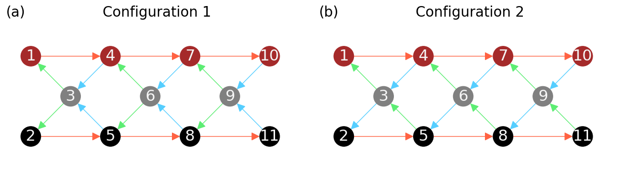
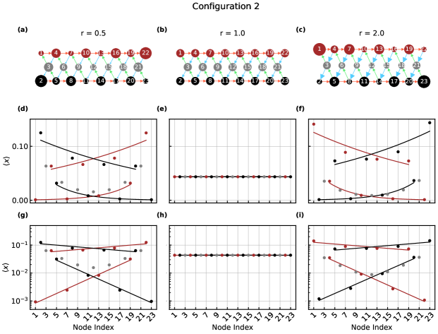
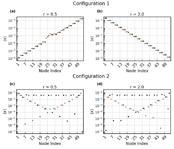
Here, we analyze the data for a graph of nodes to state the result with visual representation. The results for the larger graph are shown in the appendix B. We have divided the structure into three chains- the upper chain (i.e. node index 1, 4, 7, etc.) is marked with brown color. The middle chain (i.e. node index 3,6,9…), and the lower chain (i.e. node index 2,5,8…) are marked with gray and black color respectively. Throughout our investigation, this colour as well as the labelling scheme were maintained.
Configuration 1. .
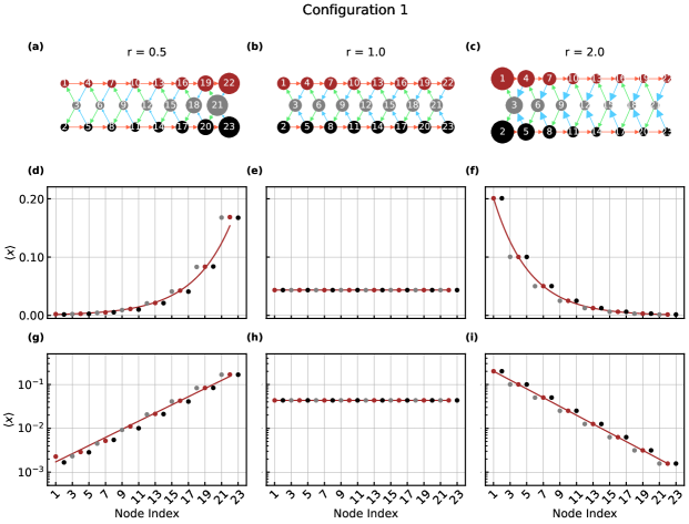
.
At first, we consider the case for (). Here, the strength of each blue link is weak compared to the others (red or green links). We observe that most of the masses are transferred to the right side of the doublet chain i.e.at node index 21, 22, and 23 (see Fig. 2(a), (d)). The density of the mass is highest in the right and then drops towards the left. This decays exponentially (Fig. 2(g), where the simulated data is replotted in semi-log scale, makes this more evident). This result is analogous to earlier works in 1-d chain Knebel et al. (2020) where mass is polarized in the right boundary when . Considering the grey nodes in this scenario, the incoming blue links are weaker than the green links. Mass can thus be transferred with ease to the upper (brown nodes) or lower surface (black nodes). Since red and green links are equally strong, all mass is progressively moved in the direction of the red links and ultimately deposited on the right side. Now, we take all the parameters as identical, i.e. (). Here, we find that the masses get uniformly distributed throughout the network (see Fig. 2(b), (e), and (h) (semi log-scale)), as all rate constants are equal. Finally, in the case of (), we observe that the average masses are highly concentrated on the left side (opposite direction to that of when ) i.e.node indexes 1,2 and 3 have a higher average density compared to others (see Fig. 2(c),(f), and (i)). The explanation is as follows: because the blue links are stronger than the green and the red links, the mass eventually shifts to the left under the influence of the direction of blue links. Here the masses are polarized in one direction, a consistent pattern with the previous work Knebel et al. (2020). It is also clear, that the highest-density nodes are times bigger than the lowest-density nodes ( as well as ). Thus, the decay constant is almost the same, as the value of in one case is reciprocal to the other case.
.
Configuration 2. Initially, () was taken into consideration. In comparison to configuration 1, we observe that the highest density is found in the network’s two opposing corners (node index 2 and 22; see Fig. 3(a), (d)). The mass is therefore not deposited on one side alone in that scenario. Additionally, red nodes are seen to follow two exponential decays. The mass decays exponentially through alternating nodes (), with node 22 having the largest accumulation of mass. Exponential decay is also followed by the other alternative set of red nodes (). Readers can examine the two red lines and the red nodes for more clarity (Fig. 3(g)). Similar behavior, but in the opposite direction, is seen in the black nodes (mass decays exponentially from 2 to 8 to 20 via 14). The identical rates () show that the masses become uniformly distributed throughout the network from a random mass distribution (see Fig. 3(b), (e), and (h)). This instance is identical to configuration 1’s. Now, where (), as opposed to the case when , we observe that masses are becoming polarized and concentrating heavily on two opposing corners of the network (node index 1 and 23) (see Fig. 3(c), (f), and (i)). Note that in configuration2, if , the middle of the gray nodes deposits comparatively less mass. Contrast to configuration 1, the directionality and strength of the links in this configuration cannot explain the average mass distribution. For instance, node 10 and 13 have same link structure, although, node 10 has strong mass deposition.
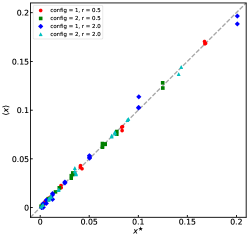
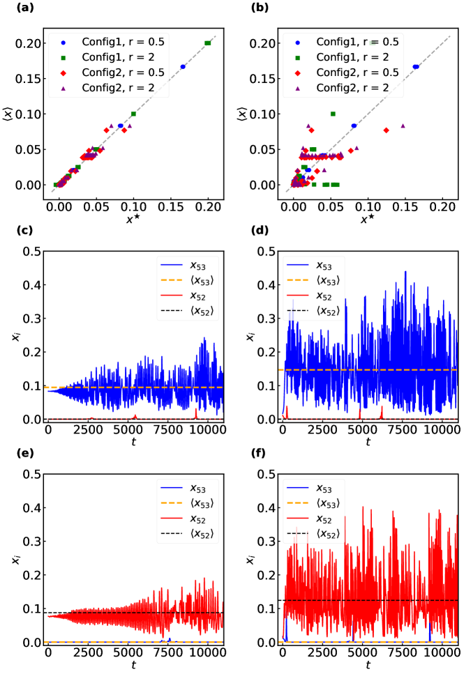
To understand this behaviour more accurately, we have checked the fixed points of these configurations. The system has one trivial fixed point vector (). Solving will yield the value of the other fixed point vector (solution: ). Upon numerically solving it, we have plotted () the average density of each site with . It is shown in Fig. 4. It can be inferred from the straight line that each node’s trajectory circles the fixed point (see Knebel et al. (2020); Reichenbach et al. (2006, 2007); Bhattacharyya et al. (2020); Chatterjee et al. (2022); Viswanathan et al. (2024); Chatterjee and Chowdhury (2024)). Additionally, we looked for a large graph (); refer to appendix B. Note that, for a large graph, we consider the initial condition as a small perturbation of the solution of . Particularly, we initially perturb with a small strength to one of the nodes. As a result, relatively large oscillation emerges, however, the average behaviour of the system can be approximated with an intrinsic non-trivial fixed point vector. Noticeably, if the perturbation is too strong or initial states are chosen randomly, the average behaviour of the nodes may not be mapped with (appendix B). It is evident now that when increases from less than 1 to greater than 1, the exponents will change sign. Is it possible to reveal phase transitions as a function of in both configurations? is a crucial question to pose. We have thoroughly examined it with analytical computation in the sections that follow. Prior to the analytical approach section, we would like to point out that, in the event that the network size is even, a unique solution for does not exist. Therefore, it is possible that the pattern of odd sizes we have observed will not show up for even sizes. This subject will be covered in greater detail in the future works. As a result, only the system size is covered by our investigation.
Analytical Approach. We now make use of the topological band theory to understand the topological properties of this RPS doublet chain Knebel et al. (2020). For this, we employ periodic boundary condition on the RPS doublet chain in Fig. 1, and write the matrix as see appendix (A) for details. Here are three block matrices, and for configuration 1, we have
| (2) |
with . Thus, becomes the block circulant, a translationally invariant matrix Gray (2006). Now, to understand our system within the framework of topological band theory, we define the RPS doublet chain Hamiltonian . The Hamiltonian constructed in this way is Hermitian with being the imaginary part of a complex number. We now analyze the spectral properties of this Hamiltonian and show that the topological properties of the doublet chain depend on the parameter . Since has transnational invariance, we can do plane wave decomposition of the eigenvectors of , and the eigenvalue equation of has the form . Here is the Fourier transformed Hamiltonian that will depend on the block matrices stated in the Eq. (2) and is given by , with Knebel et al. (2020) , being the wave number. With this, for configuration 1 has the form,
The Hamiltonian matrix for the configurations 2 is given in the appendix A. The configuration 1 and 2 have the same eigenvalues
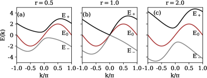
Here eigenvalues are point symmetric with respect to origin that is . This is due to the particle hole symmetry of the Hamiltonian . The energy spectrum of depends on the rate , and shown in the Fig 5. Since we have defined , we fix rates and vary the rate . Then we calculate the energy spectrum for different values of and plot them in Fig 5 (a)-(c). The eigenvalue spectra of have three energy bands for different on the Brillouin zone . We observe that the energy gap closes at as we approach and then reopens as we go away from that point. This is exactly what happens in the case of a topological phase transition Jangjan and Hosseini (2021). We can therefore label the two phases separated by to be topologically distinct.Knebel et al. (2020). In Fig 5, variation of eigenvalues is plotted against for three cases (a), (b), (c). We observe that serves as a critical value where the eigenvalues meet at one point in the Brillouin zone. The other two cases and , have a gap between two non-trivial eigenvalues that can be termed band gaps. For both configuration, we observe from the energy spectrum that we can not go from the case (a) to case (c) without going via case (b), which suggests case (a) and case (c) are two topologically distinct phases.
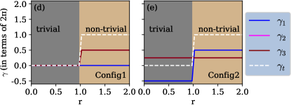
Further to identify these two distinct topological phases, we calculate the topological invariant such as winding number. For this, we calculate the Zak phase for each energy band Zak (1989), and the winding number is given by the sum of the Zak phase for all bands Yan et al. (2023); Anastasiadis et al. (2022); Jiang et al. (2018); Midya and Feng (2018) at a particular rate . The Zak phase is given by
| (3) |
where is the eigen vector for each band () Xiao et al. (2010); Zhang et al. (2021). We calculate the winding number which is the sum of the total Zak phase , shown with a white dashed line in the Fig 5 (d) - (e). We observe the topological phase transition at where the winding number change from zero to one for both configuration. Here winding number zero indicates the topological trivial phase while winding number one represents the topological non-trivial phase.
Discussion. We have studied topological phase transition in the doublet chain of RPS cycle. The considered model mimic the minimal set up of a 2D system. The mass transfer within this doublet chain is obtained by solving the ALVE equation. We have explored that for one of our configuration, the average masses are accumulated towards edges and decay exponentially consistent with results of one dimensional RPS chain. However for another configuration 2 the masses are deposited in the opposite corner and decays exponentially in an alternate way. With this we have observed the edges on both side of the RPS doublet chain, which is expected in a 2D system. The observations are robust for different network sizes and a wide range of rate parameters.
We further confirm this topological phase transition by constructing a Hamiltonian within topological band theory. We show that the energy gap between the bands closes for parameter , and for and the bands remain open. It suggests that there is a topological phase transition when system passes at . We confirm this phase transition by calculating the winding number which is the sum of Zak phases for each band. Our observation shows that the winding number is zero for trivial topological phase (), and one for non trivial topological phase ().
In the future, it will be interesting to study the 2D system by adding more layers of RPS chain in our suggested doublet chain model. However it is a highly complex problem as there will be several configurations to construct by changing the cycle of RPS chains.
Acknowledgement. We gratefully acknowledge fruitful discussions with Sahil Islam and Mauro Mobilia. R. B. acknowledges the support of the Deutsche Forschungsgemeinschaft (DFG, German Research Foundation) under Germany’s Excellence Strategy – EXC-2123 Quantum- Frontiers – 390837967.
Authors Contributions. S.C. and U.S. performed the non-linear dynamical calculations. R.B. and S.B. performed analytical and theoretical calculations. Everyone contributed to writing the paper.
References
- Thouless et al. (1982) D. J. Thouless, M. Kohmoto, M. P. Nightingale, and M. den Nijs, Phys. Rev. Lett. 49, 405 (1982).
- Jiang et al. (2012) Y. Jiang, Y. Y. Sun, M. Chen, Y. Wang, Z. Li, C. Song, K. He, L. Wang, X. Chen, Q.-K. Xue, X. Ma, and S. B. Zhang, Phys. Rev. Lett. 108, 066809 (2012).
- Haldane (1988) F. D. M. Haldane, Phys. Rev. Lett. 61, 2015 (1988).
- Kane and Lubensky (2014) C. Kane and T. Lubensky, Nature Physics 10, 39 (2014).
- Chen et al. (2016) B. G.-g. Chen, B. Liu, A. A. Evans, J. Paulose, I. Cohen, V. Vitelli, and C. D. Santangelo, Phys. Rev. Lett. 116, 135501 (2016).
- Fan et al. (2019) H. Fan, B. Xia, L. Tong, S. Zheng, and D. Yu, Phys. Rev. Lett. 122, 204301 (2019).
- Sone et al. (2020) K. Sone, Y. Ashida, and T. Sagawa, Nature communications 11, 1 (2020).
- Raghu and Haldane (2008) S. Raghu and F. D. M. Haldane, Phys. Rev. A 78, 033834 (2008).
- Ozawa et al. (2019) T. Ozawa, H. M. Price, A. Amo, N. Goldman, M. Hafezi, L. Lu, M. C. Rechtsman, D. Schuster, J. Simon, O. Zilberberg, and I. Carusotto, Rev. Mod. Phys. 91, 015006 (2019).
- He et al. (2020) L. He, Z. Addison, E. J. Mele, and B. Zhen, Nature communications 11, 1 (2020).
- Krapivsky et al. (2000) P. L. Krapivsky, S. Redner, and F. Leyvraz, Phys. Rev. Lett. 85, 4629 (2000).
- Bianconi and Barabási (2001) G. Bianconi and A.-L. Barabási, Phys. Rev. Lett. 86, 5632 (2001).
- Kaupužs et al. (2005) J. Kaupužs, R. Mahnke, and R. J. Harris, Phys. Rev. E 72, 056125 (2005).
- Evans and Waclaw (2014) M. R. Evans and B. Waclaw, Journal of Physics A: Mathematical and Theoretical 47, 095001 (2014).
- Prodan and Prodan (2009) E. Prodan and C. Prodan, Phys. Rev. Lett. 103, 248101 (2009).
- Nash et al. (2015) L. M. Nash, D. Kleckner, A. Read, V. Vitelli, A. M. Turner, and W. T. Irvine, Proceedings of the National Academy of Sciences 112, 14495 (2015).
- Souslov et al. (2017) A. Souslov, B. C. Van Zuiden, D. Bartolo, and V. Vitelli, Nature Physics 13, 1091 (2017).
- Pedro et al. (2019) R. P. Pedro, J. Paulose, A. Souslov, M. Dresselhaus, and V. Vitelli, Phys. Rev. Lett. 122, 118001 (2019).
- Yoshida and Hatsugai (2021) T. Yoshida and Y. Hatsugai, Scientific reports 11, 1 (2021).
- Knebel et al. (2020) J. Knebel, P. M. Geiger, and E. Frey, Physical Review Letters 125, 258301 (2020).
- Yoshida et al. (2022) T. Yoshida, T. Mizoguchi, and Y. Hatsugai, Scientific Reports 12, 560 (2022).
- Liang et al. (2024) J. Liang, Q. Dai, H. Li, H. Li, and J. Yang, Phys. Rev. E 110, 034208 (2024).
- Yoshida et al. (2021) T. Yoshida, T. Mizoguchi, and Y. Hatsugai, Phys. Rev. E 104, 025003 (2021).
- Vorberg et al. (2013) D. Vorberg, W. Wustmann, R. Ketzmerick, and A. Eckardt, Phys. Rev. Lett. 111, 240405 (2013).
- Chawanya and Tokita (2002) T. Chawanya and K. Tokita, Journal of the Physical Society of Japan 71, 429 (2002).
- GOEL et al. (1971) N. S. GOEL, S. C. MAITRA, and E. W. MONTROLL, Rev. Mod. Phys. 43, 231 (1971).
- May (2019) R. M. May, Stability and complexity in model ecosystems (Princeton university press, 2019).
- Di Cera et al. (1989) E. Di Cera, P. E. Phillipson, and J. Wyman, Proceedings of the National Academy of Sciences 86, 142 (1989).
- Zakharov et al. (1974) V. Zakharov, S. Musher, and A. Rubenchik, JETP Lett 19, 151 (1974).
- Manakov (1975) S. V. Manakov, Soviet Journal of Experimental and Theoretical Physics 40, 269 (1975).
- Umer and Gong (2022) M. Umer and J. Gong, Phys. Rev. B 106, L241403 (2022).
- Reichenbach et al. (2006) T. Reichenbach, M. Mobilia, and E. Frey, Phys. Rev. E 74, 051907 (2006).
- Reichenbach et al. (2007) T. Reichenbach, M. Mobilia, and E. Frey, Physical review letters 99, 238105 (2007).
- Bhattacharyya et al. (2020) S. Bhattacharyya, P. Sinha, R. De, and C. Hens, Phys. Rev. E 102, 012220 (2020).
- Chatterjee et al. (2022) S. Chatterjee, S. Nag Chowdhury, D. Ghosh, and C. Hens, Chaos: An Interdisciplinary Journal of Nonlinear Science 32 (2022).
- Viswanathan et al. (2024) K. Viswanathan, A. Wilson, S. Bhattacharyya, and C. Hens, Chaos, Solitons & Fractals 180, 114548 (2024).
- Chatterjee and Chowdhury (2024) S. Chatterjee and S. N. Chowdhury, arXiv preprint arXiv:2409.09521 (2024).
- Gray (2006) R. M. Gray, Foundations and Trends® in Communications and Information Theory 2, 155 (2006).
- Jangjan and Hosseini (2021) M. Jangjan and M. V. Hosseini, Scientific reports 11, 1 (2021).
- Zak (1989) J. Zak, Phys. Rev. Lett. 62, 2747 (1989).
- Yan et al. (2023) W. Yan, W. Cheng, W. Liu, and F. Chen, Opt. Lett. 48, 1802 (2023).
- Anastasiadis et al. (2022) A. Anastasiadis, G. Styliaris, R. Chaunsali, G. Theocharis, and F. K. Diakonos, Phys. Rev. B 106, 085109 (2022).
- Jiang et al. (2018) H. Jiang, C. Yang, and S. Chen, Phys. Rev. A 98, 052116 (2018).
- Midya and Feng (2018) B. Midya and L. Feng, Phys. Rev. A 98, 043838 (2018).
- Xiao et al. (2010) D. Xiao, M.-C. Chang, and Q. Niu, Rev. Mod. Phys. 82, 1959 (2010).
- Zhang et al. (2021) Y. Zhang, B. Ren, Y. Li, and F. Ye, Opt. Express 29, 42827 (2021).
Appendix A Antisymmetric Matrix
First, we elaborate on how can be written using the . Note that all these matrices are of the order 3X3. So, denotes a 3x3 null matrix.
Thus, is a circulant matrix and in compact form can be written as .
The corresponding anti symmetric matrix for configuration 2 is as follows:
Similarly for configuration 2 we can write, and the corresponding sub-matrices are,
Therefore the Hamiltonian matrix for configuration 2 has the form,
The behaviour of energy bands and winding number of the above Hamiltonian is discussed in the main text.
Appendix B Results in large network
Using a relatively large graph (), we have examined the mass density, confirming our observations in the main text. Fig. 6 displays the outcomes for both configurations when and are taken into account. We have selected two sets of initial conditions (IC) in order to further validate the linear relationship (): (I) From the solution , IC is selected. In two random nodes, a minor perturbation () is used. (II) Initial states are purely random. Keep in mind that we have kept the starting point at for both scenarios. We have plotted with respect to in the Fig. 7(a) (case I). In Figure 7(c), the time signals of two nodes (53 and 52) are displayed (configuration II). Node 53 exhibits irregular oscillation (blue), while Node 52 (red line) remains near zero. In this case, is set to 0.5. The average is shown by the dashed horizontal lines (after discarding the transient). When is set to 2, the opposite situation transpires (node 52 exhibits irregular oscillation and 53 remains near zero). The results for case II, in which the IC are chosen at random, are shown in Fig. 7(b), (d), and (f). Random ICs have the effect of increasing the amplitudes of the time signals (node 53 in (d), node 52 in (f)). As a result, there is some disruption in the linear relationship between and . Hence, a careful selection of initial conditions is necessary to observe the exponential decay (or strong deposition of mass density in the opposite corner). The phase transition happens at . Starting from random ICs, it has been numerically observed that (not shown here), for values of close to 1, the mass density of the configuration will be in better agreement with the solution.