Equity market dynamics are conventionally investigated in name space where stocks are indexed by company names. In contrast, by indexing stocks based on their ranks in capitalization, we gain a different perspective of market dynamics in rank space. Here, we demonstrate the superior performance of statistical arbitrage in rank space over name space, driven by a robust market representation and enhanced mean-reverting properties of residual returns in rank space. Our statistical arbitrage algorithm features an intraday rebalancing mechanism for effective conversion between portfolios in name and rank space. We explore statistical arbitrage with and without neural networks in both name and rank space and show that the portfolios obtained in rank space with neural networks significantly outperform those in name space.

1 Introduction

In equity markets, stocks are conventionally labeled by equity indices (company names). By relabeling stocks according to their ranks in capitalization, rather than their equity indices (company names), a different, more stable market structure can emerge. Specifically, we will gain a different perspective on market dynamics by focusing on the stock that occupies a certain rank in capitalization while the corresponding company name may change. We refer to a market labeled by the equity indices (company names) as a market in name space and one labeled by ranks in capitalization as a market in rank space.

Market in rank space was explored by Fernholtz et al. who observed a stable distribution of capitalization across different ranks in the U.S. equity market over different time periods[11, 16]. They further introduced an explanatory hybrid-Atlas model under stochastic portfolio theory, a framework that enables analyzing portfolios in rank space[5, 15]. Empirically, B. Healy et al. analyzed the U.S. equity data and showed that the market in rank space is driven by a dominant single factor[14], in contrast to the multi-factor-driven market in name space[9, 10, 19]. While the primary market factor in rank space has been extensively studied, the residual returns – those not explained by this primary factor in stock returns – remain a fertile land of adventure.

In addition to intellectual intrigue, the behavior of the residual returns is closely related to statistical arbitrage, a trading strategy that exploits temporary under-pricing or over-pricing of stocks. Specifically, statistical arbitrage relies on constructing market-neutral portfolios that reproduce the residual returns and make profits if the residual returns are mean-reverting. Various methodologies have been developed for designing and managing statistical arbitrage portfolios in name space, including (i) stochastic control applied to the co-integrated price processes for pairs trading, the simplest form of statistical arbitrage[21, 18, 17, 6], (ii) the parametric models that fit residuals with mean-reverting Ornstein–Uhlenbeck (OU) processes and derive the corresponding trading signals[3, 24], and (iii) deep neural networks[12]. Here, we focus on the parametric OU models and deep neural networks, because they can benefit from the diversity of multiple stocks in our investing universe and naturally extend to the statistical arbitrage in rank space.

In this paper, we show the superiority of statistical arbitrage in rank space over name space by exploiting the enhanced mean-reversion of residual returns in rank space. Our statistical arbitrage portfolios obtained using neural networks in rank space achieve an average annual return 35.68% and an average Sharpe ratio of 3.28 from 2007 to 2022 with 2 basis points transaction cost. This contrasts with the conventional statistical arbitrage in name space that yields negligible returns during the same period.

The paper is structured as follows. In section 2, we formulate the framework for statistical arbitrage in both name space and rank space. Specifically, section 2.1 addresses the market decomposition and the construction of market-neural portfolios. Section 2.2 focuses on defining and calculating trading signals and portfolio weights using either the parametric OU model or deep neural networks. Section 2.3 introduces an intraday rebalancing mechanism for effective conversion of portfolios between name space and rank space. Section 2.4 reviews the metrics for assessing the performance of the portfolios. Section 2.5 summarizes our statistical arbitrage portfolio strategies in the form of algorithms with comprehensive implementation details. In section 3 we present our empirical results within the U.S. equities market. We first demonstrate a robust market structure in rank space in section 3.2, followed by evidence of enhanced mean-reversion of residual returns in section 3.3. These lead to superior portfolio performance in rank space, especially when using neural networks, presented in section 3.4. To further understand the neural networks’ superior portfolio performance as compared to the parametric OU model, we interpreted the behavior of the neural networks in section 3.5. Finally, we estimate the characteristic time between rank switching in section 3.6, crucial for our intraday rebalancing mechanism. Section 4 summarizes the paper with concluding remarks.

2 Formulation

This section presents a detailed formulation of statistical arbitrage in name and rank space. We begin by performing market decomposition on returns using a factor model to extract the residual returns – returns not explained by market factors. This procedure applies to the conventional stock returns for name space and to rank returns in continuous-time limit for rank space. Utilizing this market decomposition, we construct market-neutral portfolios (section 2.1). With the identified residual returns, we generate the trading signals and determine portfolio weights, using either a parametric OU model[3] or deep neural networks applicable to both name space and rank space (section 2.2). Since the rank returns in the continuous-time limit do not correspond directly to tradable financial instruments, we introduce an intraday rebalancing mechanism to convert portfolio weights derived in rank space into stock-based weights (section 2.3). Finally, we evaluate the performance of various strategies by calculating the historical PnL and the associated performance metrics (section 2.4). A summary of our formulation by algorithms and schematics, along with complementary implementation details, are provided in section 2.5.

2.1 Market decomposition

Here, we delve into identifying residual returns and constructing market-neutral portfolios. We first conduct factor analysis on dividend-adjusted stock returns in name space and on rank returns in continuous-time limit in rank space. This analysis yields a linear transformation that maps between the equity space and the residual space, enabling a straightforward construction of market-neural portfolios.

2.1.1 Name space

In a market consisting of $N$ stocks, we denote the dividend-adjusted return on stock $i$ at trading day $t$ by $r_{i,t}$. We adopt a factor model for stock return,

$$r_{t}-r_{f}=\beta_{t}F_{t}+\epsilon_{t},\quad\quad t=1,2,...,T$$ (2.1.1)

. Here, $r_{t}=\{r_{i,t}\}_{i=1}^{N}\in\mathbb{R}^{N}$ are the dividend-adjusted daily return, $r_{f}\in\mathbb{R}$ is the risk-free rate, $F_{t}\in\mathbb{R}^{K\times 1}$ are the underlying factors, $\beta_{t}\in\mathbb{R}^{N\times K}$ are the corresponding loadings on $K$ factors, and $\epsilon_{t}\in\mathbb{R}^{N}$ are the residual returns. Factor candidates varies widely, ranging from economical-driven factors such as the Fama-French factors[9, 10], to statistically-driven factors derived from PCA[3]. In our approach, factors are selected as the leading eigenvectors in PCA[3, 24]. The number of factors $K$ is chosen based on the eigenvalue spectrum of the empirical correlation of daily returns (Fig. 6(c1-c6)).

Without loss of generality, these factors can be interpreted as portfolios of stocks,

$$F_{t}=\omega_{t}(r_{t}-r_{f})$$ (2.1.2)

, where $\omega_{t}\in\mathbb{R}^{K\times N}$ contains corresponding portfolio weights. Eq. 2.1.1 and Eq. 2.1.2 give

$$r_{t}-r_{f}=\beta_{t}\omega_{t}(r_{t}-r_{f})+\epsilon_{t}\Rightarrow\epsilon_{t}=(I-\beta_{t}\omega_{t})(r_{t}-r_{f}):=\Phi_{t}(r_{t}-r_{f})$$ (2.1.3)

. Here,

$$\Phi_{t}:=(I-\beta_{t}\omega_{t})$$ (2.1.4)

defines a linear transformation from $r_{t}$ to $\epsilon_{t}$. More importantly, $\epsilon_{i,t}$ can be viewed as the return of a tradable portfolio with weights specified by the $i$-th row of $\Phi_{t}$. Consequently, the investing universe spanned by $r_{t}$ is termed as name equity space, and that spanned by $\epsilon_{t}$ as name residual space.

We denote the portfolio weights in name equity space as $w_{t}^{R,\text{name}}$ and portfolio weights in name residual space as $w_{t}^{\epsilon,\text{name}}$. These weights are related by

$$w_{t}^{R,\text{name}}=\Phi_{t}^{T}w_{t}^{\epsilon,\text{name}}$$ (2.1.5)

, directly following the equality in portfolio return,

$$(w_{t}^{\epsilon,\text{name}})^{T}\epsilon_{t}=(w_{t}^{\epsilon,\text{name}})^{T}\Phi_{t}(r_{t}-r_{f})=(w_{t}^{R,\text{name}})^{T}(r_{t}-r_{f})$$ (2.1.6)

For factors derived by PCA, we have

$$\Phi_{t}\beta_{t}=0\implies(w_{t}^{R,\text{name}})^{T}\beta_{t}=(w_{t}^{\epsilon,\text{name}})^{T}\Phi_{t}\beta_{t}=0,\quad\forall w_{t}^{\epsilon,\text{name}}$$ (2.1.7)

, with proof given in the appendix. It means that for any $w_{t}^{\epsilon,\text{name}}$, the $w_{t}^{R,\text{name}}$ calculated by Eq. 2.1.5 satisfy,

$$(w_{t}^{R,\text{name}})^{T}(r_{t}-r_{f})=(w_{t}^{\epsilon,\text{name}})^{T}\Phi_{t}(\beta_{t}F_{t}+\epsilon_{t})=(w_{t}^{\epsilon,\text{name}})^{T}\Phi_{t}\epsilon_{t}=(w_{t}^{R,\text{name}})^{T}\epsilon_{t}$$ (2.1.8)

It suggests that the return of our statistical arbitrage portfolios is independent of market factors and relies solely on residual returns, a property usually termed as market neutrality[3, 24]. Ideally, portfolios are also desired to have a zero net value, known as dollar neutrality. Empirical evidence suggests that market-neutral portfolios are also approximately dollar-neutral (Fig. 15).

2.1.2 Rank space

We initiate our formulation for market decomposition in rank space by introducing key notations. Let $c_{i,t}$ denote the capitalization of stock $i$ at day $t$, and $c_{(k),t}$ represent the capitalization of stock which occupies $k$-th rank in descending order at day $t$. Additionally, $\mathcal{R}_{i,t}$ represents the rank in capitalization for stock $i$ at day $t$, and $\mathcal{I}_{(k),t}$ represents the stock index (name) that occupies the rank $k$ at day $t$. We define the daily return on rank $k$ at day $t$ in the continuous-time limit as $\tilde{r}_{(k),t}$, that

$$\tilde{r}_{(k),t}:=\frac{c_{(k),t}-c_{(k),t-1}}{c_{(k),t-1}}=\frac{c_{\mathcal{I}_{(k),t},t}-c_{\mathcal{I}_{(k),t-1},t-1}}{c_{\mathcal{I}_{(k),t-1},t-1}}$$ (2.1.9)

Notably, $\tilde{r}_{t}$ does not necessarily correspond to direct financial quantity because stock names occupying rank $k$ may be different between day $t$ and $t-1$ (i.e. $\mathcal{I}_{(k),t}\neq\mathcal{I}_{(k),t-1}$). The realization of $\tilde{r}_{t}$ poses a critical challenge, which will be further elaborated in the section 2.3. Nevertheless, we assume a factor model for $\tilde{r}_{t}$ parallel to name space:

$$\tilde{r}_{t}-r_{f}=\tilde{\beta_{t}}\tilde{F_{t}}+\tilde{\epsilon}_{t}$$ (2.1.10)

, where $\tilde{r}_{t}=\{r_{(k),t}\}_{k=1}^{N}\in\mathbb{R}^{N}$, $\tilde{\beta_{t}}\in\mathbb{R}^{N\times K}$, $\tilde{F_{t}}\in\mathbb{R}^{K\times 1}$, and $\tilde{\epsilon}_{t}\in\mathbb{R}^{N}$. Following a similar transformation as in name space, we have:

$$\tilde{r}_{t}-r_{f}=\tilde{\beta}_{t}\tilde{\omega}_{t}(\tilde{r}_{t}-r_{f})+\tilde{\epsilon}_{t}\Rightarrow\tilde{\epsilon}_{t}=(I-\tilde{\beta}_{t}\tilde{\omega}_{t})(\tilde{r}_{t}-r_{f}):=\tilde{\Phi}_{t}(\tilde{r}_{t}-r_{f})$$ (2.1.11)

, where

$$\tilde{\Phi}_{t}:=(I-\tilde{\beta}_{t}\tilde{\omega}_{t})$$ (2.1.12)

defines a linear transformation from $\tilde{r}_{t}$ to $\tilde{\epsilon}_{t}$. Remarkably, if $\tilde{r}_{t}$ becomes realizable, the $\tilde{\epsilon}_{i,t}$ will also become the return of a tradable portfolio with weights on the artificial financial instruments realizing $\tilde{r}_{t}$ given by the $i$-th row of $\tilde{\Phi}_{t}$. Consequently, we define the investing universe spanned by $\tilde{r}_{t}$ as rank equity space and that spanned by $\tilde{\epsilon}_{t}$ as rank residual space, echoing our definition in the name space. The portfolio weights in rank equity space are denoted as $w_{t}^{R,\text{rank}}$ and that in rank residual space as $w_{t}^{\epsilon,\text{rank}}$. From similar reasoning in name space, these weights are related by

$$w_{t}^{R,\text{rank}}=\tilde{\Phi}_{t}^{T}w_{t}^{\epsilon,\text{rank}}$$ (2.1.13)

, and therefore,

$$(w_{t}^{R,\text{rank}})^{T}\beta_{t}=(w_{t}^{\epsilon,\text{rank}})^{T}\tilde{\Phi}_{t}\beta_{t}=0,\quad\forall w_{t}^{\epsilon,\text{rank}}$$ (2.1.14)

. This suggests that the constructed portfolios in rank space satisfy market neutrality and consequently approximate dollar neutrality, similar to those in name space.

2.2 Trading signals and portfolio weights

Despite that the residual returns $\epsilon_{t}$ or $\tilde{\epsilon}_{t}$ may be calculated in either name space or rank space, deriving the corresponding trading signal and portfolio weights takes a unified framework, which we elaborate on in this section. We first define the cumulative residual returns $x_{t}^{L}$ as

$$x_{t}^{L}=(x_{t-L+1},x_{t-L+2},...,x_{t})$$ (2.2.1)

, where

$$x_{t-L+\alpha}=\sum_{j=1}^{\alpha}\epsilon_{t-L+j},\quad\alpha=1,2,...,L$$ (2.2.2)

for name space and

$$\tilde{x}_{t-L+\alpha}=\sum_{j=1}^{\alpha}\tilde{\epsilon}_{t-L+j},\quad\alpha=1,2,...,L$$ (2.2.3)

for rank space. The cumulative residual returns $x_{t}^{L}$ and $\tilde{x}_{t}^{L}$ are used to calculate $w_{t}^{\epsilon}$ in name space and rank space, respectively. In the following, we focus on two approaches to calculate $w_{t}^{\epsilon}$: (i) a parametric model based on OU process[3, 24], and (ii) deep neural networks[12] that combine the convolutional neural networks (CNN)[20] with transformers[23, 7].

2.2.1 Parametric model: OU process

Our parametric model follows closely to the framework proposed by Avellaneda and Lee[3]. This model applies to both name space and rank space, depending on whether $x_{t}^{L}$ or $\tilde{x}_{t}^{L}$ is chosen as the input. We first fit $x_{t}^{L}$ to an OU process $X_{t}$ governed by the stochastic differential equation

$$dX_{t}=\frac{1}{\tau}(\mu-X_{t})dt+\sigma dB_{t}$$ (2.2.4)

, where $\tau$ is the mean-reverting time, $\mu$ is the long-term average of $X_{t}$, $B_{t}$ is the standard Brownian motion, and $\sigma$ is its volatility. Subsequently, we calculate the trading signal in name space

$$s^{\text{OU}}_{i,t}=\frac{x_{i,t}-\hat{\mu}_{i}}{\hat{\sigma_{i}}}$$ (2.2.5)

, where $\hat{\mu}_{i},\hat{\sigma}_{i}$ are the maximum likelihood estimator of $\mu$ and $\sigma$[3] and $x_{i,t}$ is the terminal cumulative residual return at time $t$,

$$x_{i,t}=\sum_{j=1}^{L}\epsilon_{i,t-L+j}$$ (2.2.6)

. We also include the estimated mean-reverting time $\hat{\tau}$ to effectively filter the trading opportunities[24]. The details of parameter estimation are presented in the appendix. We open short/long positions when observing large positive/negative signals and close positions when the trading signals mean-revert close to zero (schematic in Fig. 1). Following the principle, the portfolio weights in residual space, $w_{t}^{\epsilon|\text{OU},\text{name/rank}}$ become

$$w_{i,t}^{\epsilon|\text{OU},\text{name/rank}}=\begin{cases}-1,&\text{if}\quad w_{i,t-1}^{\epsilon|\text{OU}}=0,\quad s_{i,t}^{\text{OU}}>c_{\text{thresh-open}},\quad\hat{\tau_{i}}<30\text{ days}\\ 1,&\text{if}\quad w_{i,t-1}^{\epsilon|\text{OU}}=0,\quad s_{i,t}^{\text{OU}}<-c_{\text{thresh-open}},\quad\hat{\tau_{i}}<30\text{ days}\\ 1,&\text{if}\quad w_{i,t-1}^{\epsilon|\text{OU}}=1,\quad s_{i,t}^{\text{OU}}>c_{\text{thresh-close}},\quad\hat{\tau_{i}}<30\text{ days}\\ -1,&\text{if}\quad w_{i,t-1}^{\epsilon|\text{OU}}=-1,\quad s_{i,t}^{\text{OU}}>c_{\text{thresh-close}},\quad\hat{\tau_{i}}<30\text{ days}\\ 0,&\text{otherwise}\end{cases}$$ (2.2.7)

For our back-testing, the parameters are set as follows:

$$c_{\text{thresh-open}}=1.25,\quad c_{\text{thresh-close}}=0.5$$ (2.2.8)

, in accordance with [3, 24]. After calculating $w_{t}^{\epsilon|\text{OU},\text{name/rank}}$, the conversion to portfolio weights in equity space, $w_{t}^{R|\text{OU},\text{name/rank}}$, straightforwardly follow the Eq. 2.1.5 in name space

$$w_{t}^{R|\text{OU},\text{name}}=\Phi_{t}^{T}w_{t}^{\epsilon|\text{OU},\text{name}}$$ (2.2.9)

and from Eq. 2.1.13 in rank space,

$$w_{t}^{R|\text{OU},\text{rank}}=\tilde{\Phi}_{t}^{T}w_{t}^{\epsilon|\text{OU},\text{name}}$$ (2.2.10)

. The practical implementation of the parametric model is summarized in Algorithm 2 along with a schematic in panel (d1, e1) in Fig. 5.

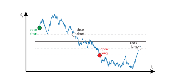
Figure 1: Schematic for the parametric model. The blue line shows the trading signal $s_{t}$. We open short/long positions when observing large positive/negative signals and close positions when the trading signals mean-revert to zero.

2.2.2 Deep neural networks

As an alternative to the parametric OU model, we adopt deep neural networks as a data-driven method to calculate portfolio weights in residual space $w_{t}^{\epsilon}$ for both name space and rank space. Specifically, the input of the neural networks is the cumulative residual returns $x_{t}^{L}$ and the output of the neural networks is $w_{t}^{\epsilon|\text{NN, name/rank}}$,

$$\mathcal{N}:x_{t}^{L}\rightarrow w_{t}^{\epsilon|\text{NN, name}}$$ (2.2.11)

for name space and

$$\mathcal{N}:\tilde{x}_{t}^{L}\rightarrow w_{t}^{\epsilon|\text{NN, rank}}$$ (2.2.12)

for rank space. The neural networks are trained similarly in both name and rank space through mean-variance optimization,

$$\text{Maximize}_{\mathcal{N}(\cdot)} \mathbb{E}[(w_{t}^{R|\text{NN},\text{name}})^{T}(r_{t+1}-r_{f})]-\gamma\text{Var}[(w_{t}^{R|\text{NN},\text{name}})^{T}(r_{t+1}-r_{f})]$$ (2.2.13)

s.t. $$w_{t}^{R|\text{NN},\text{name}}=\frac{\Phi_{t}^{T}w_{t}^{\epsilon|\text{NN},\text{name}}}{||\Phi_{t}^{T}w_{t}^{\epsilon|\text{NN},\text{name}}||_{1}}$$

$$w_{t}^{\epsilon|\text{NN},\text{name}}=\mathcal{N}(x_{t}^{L})$$

in name space and

$$\text{Maximize}_{\mathcal{N}(\cdot)} \mathbb{E}[(w_{t}^{R|\text{NN},\text{rank}})^{T}(\tilde{r}_{t+1}-r_{f})]-\gamma\text{Var}[(w_{t}^{R|\text{NN},\text{rank}})^{T}(\tilde{r}_{t+1}-r_{f})]$$ (2.2.14)

s.t. $$w_{t}^{R|\text{NN},\text{rank}}=\frac{\tilde{\Phi}_{t}^{T}w_{t}^{\epsilon|\text{NN},\text{rank}}}{||\tilde{\Phi}_{t}^{T}w_{t}^{\epsilon|\text{NN},\text{rank}}||_{1}}$$

$$w_{t}^{\epsilon|\text{NN},\text{rank}}=\mathcal{N}(\tilde{x}_{t}^{L})$$

in rank space. $\gamma$ is the risk-aversion factor. The empirical expectation and variance are obtained over a consecutive time window of length $T$,

$$\mathbb{E}[(w_{t}^{R|\text{NN}})^{T}(r_{t+1}-r_{f})] \approx\frac{1}{T}\sum_{\alpha=1}^{T}(w_{t+\alpha}^{R|\text{NN}})^{T}(r_{t+\alpha+1}-r_{f})$$ (2.2.15)

$$\text{Var}[(w_{t}^{R|\text{NN}})^{T}(r_{t+1}-r_{f})] \approx\frac{1}{T}\sum_{\alpha=1}^{T}[(w_{t+\alpha}^{R|\text{NN}})^{T}(r_{t+\alpha+1}-r_{f})-\mathbb{E}((w_{t}^{R|\text{NN}})^{T}(r_{t+1}-r_{f}))]^{2}$$

. The problems here share a similar spirit to the Markowitz portfolio optimization[1]. In our empirical analysis, we choose the risk-aversion factor $\gamma=2$ and length of time window $T=24$ days.

With $w_{t}^{\epsilon|\text{NN},\text{name/rank}}$ as the output from the neural network, the portfolio weights in equity space $w_{t}^{R|\text{NN},\text{name/rank}}$ is seemingly integrated using Eq. 2.1.5 in name space

$$w_{t}^{R|\text{NN},\text{name}}=\Phi_{t}^{T}w_{t}^{\epsilon|\text{NN},\text{name}}$$ (2.2.16)

and using Eq. 2.1.13 in rank space,

$$w_{t}^{R|\text{NN},\text{rank}}=\tilde{\Phi}_{t}^{T}w_{t}^{\epsilon|\text{NN},\text{rank}}$$ (2.2.17)

. The practical implementation of the parametric model is summarized in Algorithm 3 along with a schematic in panel (d2, e2) in Fig. 5.

In the following, we delve into the specific architecture of our neural networks, illustrated in Fig. 2. Our CNN-transformer architecture harnesses the strengths of CNN in extracting local patterns and transformers in capturing long-term dependencies. The inputs of our neural networks are the trajectories of cumulative residual returns, $x_{t}^{L}\in\mathbb{R}^{N\times L}$, processed through two layer of multi-channel convolutional networks, followed by a standard transformer encoder layer that models global relationships via multi-head attention. Specifically, in the convolutionary layer,

$$x_{t}^{(1)} =\frac{x_{t}^{L}-\mathbb{E}(x_{t}^{L})}{\sqrt{\text{Var}(x_{t}^{L})+\epsilon}}\times\gamma^{(1)}+\beta^{(1)},\quad y_{t}^{(1)}=W^{(1)}*x_{t}^{(1)}+b^{(1)},\quad z_{t}^{(1)}=\text{ReLu}(y_{t}^{(1)})+x_{t}^{(1)};$$ (2.2.18)

$$x_{t}^{(2)} =\frac{z_{t}^{(1)}-\mathbb{E}(z_{t}^{(1)})}{\sqrt{\text{Var}(z_{t}^{(1)})+\epsilon}}\times\gamma^{(2)}+\beta^{(2)},\quad y_{t}^{(2)}=W^{(2)}*x_{t}^{(2)}+b^{(2)},\quad z_{t}^{(2)}=\text{ReLu}(y_{t}^{(2)})+x_{t}^{(2)}$$

. The superscript $(1)$ or $(2)$ specifies the layer number. $x_{t}^{(1)}\in\mathbb{R}^{N\times L}$ is the input of the first convolutional layer. $W^{(1)}\in\mathbb{R}^{D_{\text{channel}}\times 1\times D_{\text{kernel}}}$ and $W^{(2)}\in\mathbb{R}^{D_{\text{channel}}\times D_{\text{channel}}\times D_{\text{kernel}}}$ are the convolutionary kernels for the convolution operator denoted by $*$, $b^{(1,2)}\in\mathbb{R}^{D_{\text{channel}}}$ is the bias, and $y_{t}^{(1,2)}\in\mathbb{R}^{N\times D_{\text{channel}}\times L}$ is the output of convolutionary operator. $D_{\text{channel}}$ is the number of channels and $D_{\text{kernel}}$ is the size of the convolution kernel. We adopt a rectified linear unit (denoted as ReLu($\cdot$)) as our activation function. We also apply (i) instance normalization [22] with learnable parameter $\gamma^{(1,2)}$ and $\beta^{(1,2)}$ at the input of each convolution layer to accelerate the training process, and (ii) residual connection[13] to avoid vanishing gradients by directly connecting the input $x_{t}^{(1,2)}$ to the output $z_{t}^{(1,2)}\in\mathbb{R}^{N\times D_{\text{channel}}\times T}$. We choose the hyper-parameters for our neural networks as number of channels $D_{\text{channel}}=8$ and size of the convolution kernel $D_{\text{kernel}}=2$.

The outputs of convolutionary layers, $z_{t}^{(2)}\in\mathbb{R}^{N\times D_{\text{channel}}\times T}$ are subsequently fed into a standard transformer encoder layer[23]. The transformer encoder layer utilizes the multi-head attention modeled by the inner product between the famous key-query-value matrices. To elaborate,

$$x_{t}^{\text{transformer}}=(z_{t}^{(2)})^{T}$$ (2.2.19)

$$\begin{cases}Q_{i}&=\text{DropOut}(W_{i}^{Q}x_{t}^{\text{transformer}}+b_{i}^{Q})\\ K_{i}&=\text{DropOut}(W_{i}^{K}x_{t}^{\text{transformer}}+b_{i}^{K})\\ V_{i}&=\text{DropOut}(W_{i}^{V}x_{t}^{\text{transformer}}+b_{i}^{V})\end{cases},\quad i=1,2,...,H$$

$$\text{head}_{i}=\text{softmax}(\frac{Q_{i}K_{i}^{T}}{\sqrt{d_{\text{channel}}/H}}),\quad i=1,2,...,H$$

$$y_{t}=\text{Concat}(\text{head}_{1}V_{1},...,\text{head}_{H}V_{H})$$

$$z_{t}=\text{LayerNorm}(x_{t}^{\text{transformer}}+y_{t})$$

$$o_{t}=\text{LayerNorm}(W^{O}z_{t}+b^{O}+y_{t})$$

, where $x_{t}^{\text{transformer}}\in\mathbb{R}^{N\times T\times D_{\text{channel}}}$ is the input of the transformer encoder layer. In addition, $W_{i}^{Q}\in\mathbb{R}^{(D_{\text{channel}}/H)\times D_{\text{channel}}}$, $W_{i}^{K}\in\mathbb{R}^{(D_{\text{channel}}/H)\times D_{\text{channel}}}$, and $W_{i}^{V}\in\mathbb{R}^{D_{(\text{channel}}/H)\times D_{\text{channel}}}$ are the linear weights. $b_{i}^{Q}\in\mathbb{R}^{D_{\text{channel}}/H}$, $b_{i}^{K}\in\mathbb{R}^{D_{\text{channel}}/H}$, and $b_{i}^{V}\in\mathbb{R}^{D_{\text{channel}}/H}$ are the bias. Softmax($\cdot$) stands for softmax function and Concat($\cdot$) for matrix concatenation, and $y_{t}\in\mathbb{R}^{N\times T\times D_{\text{channel}}}$ is the output of multi-attention layer. $W^{O}\in\mathbb{R}^{D_{\text{channel}}\times D_{\text{channel}}}$ and $b^{O}\in\mathbb{R}^{D_{\text{channel}}}$ are the linear weights and bias in the output linear layer. $o_{t}\in\mathbb{R}^{N\times T\times D_{\text{channel}}}$ is the output of the transformer. In addition to the residual connection similar to the convolutional layer, we also introduce the drop-out technique, denoted as Dropout($\cdot$), to regularize overfitting with drop-out probability $p$, and layer normalization[4], denoted as LayerNorm($\cdot$), to improve training stability. We choose the hyper-parameters for our neural networks as the number of heads $H=4$ and the drop-out probability $p=0.25$.

Finally, we choose the last slice along the time axis in the output of the transformer, $o_{t}\in\mathbb{R}^{N\times T\times D_{\text{channel}}}$, as the hidden state summarizing the information up to time $t$. The portfolio weights in residual space $w_{t}^{\epsilon|\text{NN},\text{name/rank}}$ are calculated by a linear relationship,

$$w_{t}^{\epsilon|\text{NN},\text{name/rank}}=W^{F}(o_{t}[\text{:, -1, :}])+b^{F}$$ (2.2.20)

, where $o_{t}[\text{:, -1, :}]\in\mathbb{R}^{N\times D_{\text{channel}}}$ means the last slice along the second-dimension (time-axis) of $o_{t}$, and $W^{F}\in\mathbb{R}^{1\times D_{\text{channel}}}$, $b^{F}\in\mathbb{R}$ are the parameters.

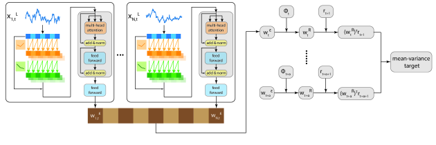
Figure 2: Schematic for the architecture of neural networks in both name and rank space. The input of the neural networks is the trajectory of the cumulative residual returns at trading day $t$, calculated by the market decomposition from either name space or rank space. The trajectories are subsequently fed into (i) multi-channel convolutional layers to extract local patterns, (ii) a classical transformer encoding layer for global attention, and (iii) a feed-forward network. The output is the portfolio weights in residual space, $w_{t}^{\epsilon}$. The portfolio weights in equity space $w_{t}^{R}$ are derived directly from $w_{t}^{\epsilon}$ using the transformation $w_{t}^{\epsilon}$ by $w_{t}^{R}=\Phi_{t}^{T}w_{t}^{\epsilon}$, with $l_{1}$ normalization. The portfolio returns at trading day $t+1$ then becomes $(w_{t}^{R})^{T}r_{t+1}$, and similar calculations are carried out for subsequent days. These returns are used to estimate the mean and variance of the portfolio’s performance. Finally, neural networks update their parameters by optimizing the mean-variance target. The gradients of the parameters are calculated using backpropagation with adaptive moment estimation[8].

2.3 intraday rebalancing

Notably, the portfolio weights calculated in the rank space are assigned to artificial financial instruments that yield rank returns in continuous-time limits. For practical implementation, it is necessary to convert these portfolio weights into stock-based portfolios.

A natural approach is to assign the portfolio weights with correspondence between ranks and names at the end of each trading day and hold the portfolio throughout the following trading day,

$$w_{i,t}=\sum_{k=1}^{N}w_{(k),t}\boldsymbol{1}_{\{\mathcal{R}_{i,t}=k\}},\quad\quad i=1,2,...,N$$ (2.3.1)

. Unfortunately, this straightforward conversion will not retain the advantages of statistical arbitrage in rank space, because the performance of the derived portfolio will essentially still depend on returns in name space rather than the rank returns in continuous-time limit. As indicated by Eq. 2.1.9, the returns in name and rank space start to diverge in the event of rank switching that frequently occurs for most ranks at an intraday frequency. It indicates that an effective conversion strategy must appropriately respond to the rank-switching events.

Consequently, we propose an intraday rebalancing mechanism. This mechanism performs conversion from rank space to name space at a frequency that matches rank-switching events, even though it results in higher transaction costs due to more frequent trading. The detailed formulation is provided in section 2.3.1, complemented by Algorithm 4. In section 2.3.2, we perform an in-depth analysis of the intraday rebalancing mechanism applied to a two-stock system, emphasizing the crucial role of rank switching and the rebalancing interval in determining the cost of conversion.

2.3.1 Conversion weights from rank space to name space

Here, we explain our intraday rebalancing mechanism. Formally, given the predetermined portfolio weights in rank equity space $\{w_{(k),t}^{\text{rank}}\}_{k=1}^{N}$ before the market opening, our goal is to rebalance the portfolio at fixed time intervals of $\mathcal{T}$ minutes such that the portfolio becomes $\{w_{(k),t}^{\text{rank}}(1+\tilde{r}_{(k),t+1})\}_{k=1}^{N}$ by market close, at the sacrifice of additional costs. To facilitate this discussion, we introduce two processes:

(i) $w_{(k),t+\tau}^{\text{rank}}$: the dollar-valued portfolio weight for rank $k$ at time $t+\tau$;

(ii) $w_{i,t+\tau}^{\text{name}}$: the dollar-valued portfolio weight for stock $i$ at time $t+\tau$.

Here, $t$ denotes the daily time tick and $\tau$ represents the intraday time tick. For instance, for $t=$ Jan, 3rd, 2022 (end of the day) and $\tau=45$ minutes, $t+\tau$ refers to Jan, 4th, 2022 00:45 AM, and $t+1$ refers to the end of the day on Jan, 4th, 2022.

$w_{(k),t+\tau}^{\text{rank}}$ is the portfolio weight on the $k$-th rank that evolves strictly based on the rank returns in continuous-time limit,

$$w_{(k),t+\tau}^{\text{rank}}=w_{(k),t}^{\text{rank}}(1+\tilde{r}_{(k),t+\tau})$$ (2.3.2)

, where

$$\tilde{r}_{(k),t+\tau}=\frac{c_{(k),t+\tau}}{c_{(k),t}}-1$$ (2.3.3)

. Here, $c_{(k),t+\tau}$ denotes the $k$-th rank capitalization at time $t+\tau$.

In contrast, $w_{i,t+\tau}^{\text{name}}$ is the portfolio weight on the $i$-th stock, evolving according to the following rules:

(i) Between the rebalancing interval when $t+j\mathcal{T}<t+\tau\leq t+(j+1)\mathcal{T},j\in\mathbb{N}$,

$$w_{i,t+\tau}^{\text{name}}=w_{i,t+(j\mathcal{T})^{+}}^{\text{name}}\times\frac{c_{i,t+\tau}}{c_{i,t+(j\mathcal{T})^{+}}}$$ (2.3.4)

, where $(j\mathcal{T})^{+}:=\lim_{\delta\downarrow 0}(j\mathcal{T}+\delta)$.

(ii) At the re-balancing point when $\tau=((j+1)\mathcal{T})^{+},j\in\mathbb{N}$, adjust the portfolio weights via active trading such that

$$w_{i,t+((j+1)\mathcal{T})^{+}}^{\text{name}}=w_{(k),t+(j+1)\mathcal{T}}^{\text{rank}},\quad\text{if}\quad\mathcal{R}_{i,t+(j+1)\mathcal{T}}=k$$ (2.3.5)

. In other words, we carry out the conversion of portfolio weights between name space and rank space at the rebalancing point through active trading. Notably, the value on the trading book before trading at $t+(j+1)\mathcal{T}$ is $\sum_{k=1}^{N}w_{i,t+(j+1)\mathcal{T}}^{\text{name}}$ and the desired value immediately after trading is $\sum_{i=1}^{N}w_{i,t+(j+1)\mathcal{T}^{+}}^{\text{name}}=\sum_{k=1}^{N}w_{(k),t+(j+1)\mathcal{T}}^{\text{rank}}$. The two values are not necessarily equal when there exists switching of ranks in capitalization between $t+j\mathcal{T}$ and $t+(j+1)\mathcal{T}$, which we will elaborate by a case study in section 2.3.2. Consequently, the cost of the active trading at $t+(j+1)\mathcal{T}$ involves two components,

$$\text{cost}(t+(j+1)\mathcal{T}^{+};w_{(k),t}^{\text{rank}})= (\sum_{i=1}^{N}w_{i,t+(j+1)\mathcal{T}^{+}}^{\text{name}}-\sum_{k=1}^{N}w_{(k),t+(j+1)\mathcal{T}}^{\text{rank}})$$ (2.3.6)

$$+\eta\sum_{i=1}^{N}|w_{i,t+(j+1)\mathcal{T}^{+}}^{\text{name}}-w_{i,t+(j+1)\mathcal{T}}^{\text{name}}|$$

, where $\eta$ is the transaction cost factor.

Remarkably, the cost at time $t+(j+1)\mathcal{T}^{+}$ depends on the portfolio weights assigned at the beginning of the trading day, $w_{(k),t}^{\text{rank}}$, because the intraday portfolio weights $w_{i,t+\tau}^{\text{name}}$ and $w_{(k),t+\tau}^{\text{rank}}$ are recursively governed by the system dynamics (Eq. 2.3.2, Eq. 2.3.4, and Eq. 2.3.5) from the initial condition $w_{(k),t}^{\text{rank}}$. We highlight this dependence by including the $w_{(k),t}^{\text{rank}}$ as a parameter for the cost in Eq. 2.3.6. We refer to the first term in Eq. 2.3.6 as latency cost, the second term as cost from the bid-ask spread, with their sum representing the total transaction cost. The terminology will be rationalized in the following case study.

The precise implementation of the intraday rebalancing is summarized in Algorithm 4 along with a schematic in panel (f3) in Fig. 5. For our backtesting, we primarily use $\eta=2$ basis points to account for the cost from the bid-ask spread. This setting approximately corresponds to a 5-10 cents bid-ask spread for our investment universe, the top 500 stocks in the U.S. equity market. We will discuss the impact of $\eta$ on portfolio performance dependence in section 3.7.

2.3.2 Portfolio rebalancing through rank switching of two stocks

To elucidate the pivotal role of rank switching in our intraday rebalancing strategy, we examine a two-stock system depicted in Fig. 3, where the two capitalization processes $c_{t,1}$ and $c_{t,2}$ maintain their ranks during the rebalancing interval $((k-1)\mathcal{T},k\mathcal{T}],k\in\mathbb{N}$ and swap their ranks during $(k\mathcal{T},(k+1)\mathcal{T}],k\in\mathbb{N}$ (panels (a1-a7)). The red lines in panels (b1-b7) and green lines in panels (c1-c7) show the dollar portfolio weight on the stock that occupies $k$-th rank in capitalization, $w_{(k),\tau},k=1,2$. The orange lines in panels (b1-b7) and blue lines in panels (c1-c7) show the dollar portfolio weight on the stock that has $i$-th name index, $w_{i,\tau},i=1,2$. We further calculate and present in panels (d1-d7) the divergence between the total dollar portfolio weights in rank space and the total dollar portfolio weights in name space, defined as $w_{(1),t}+w_{(2),t}-w_{1,t}-w_{2,t}$. Panels (e1-e7) shows the cumulative cost from the bid-ask spread arising from the active trading at the rebalancing point. We highlight several representative timestamps elaborated below.

(i) $t=(k-1)\mathcal{T}^{+}$ in panels (a1-e1): We invest $w_{(2),t}$ on stock 1 and $w_{(1),t}$ on stock 2 since $c_{1,t}<c_{2,t}$. Therefore, $w_{(1),t}=w_{2,t}$ and $w_{(2),t}=w_{1,t}$;

(ii) $t=k\mathcal{T}$ in panel (a2-e2): The processes evolve towards the rebalancing point $k\mathcal{T}$. The relationship $w_{(1),t}=w_{2,t},w_{(2),t}=w_{1,t}$ maintains because there is no rank-swapping between stock 1 and stock 2;

(iii) $t=k\mathcal{T}^{+}$ in panels (a3-e3): At the rebalancing point, no active trading is needed as $w_{(1),t}=w_{2,t},w_{(2),t}=w_{1,t}$ for $i=1,2$, and therefore no divergence (latency cost) or cost from bid-ask spread incurred;

(iv) $k\mathcal{T}<t\leq(k+1)\mathcal{T}$ in panels (a4-e4, a5-e5): The processes evolve towards the rebalancing point $(k+1)\mathcal{T}$. However, because of the rank switch in capitalization between stock 1 and 2 during the interval, the dollar-valued portfolio for rank and the dollar-valued portfolio for name start diverging, i.e. $w_{(1),t}\neq w_{2,t},w_{(2),t}\neq w_{1,t}$ and reaches a maximum at the next rebalancing point $(k+1)\mathcal{T}$ (panel (d4, d5));

(v) $t=(k+1)\mathcal{T}^{+}$ in panels (a6-e6): We carry out active trading to rebalancing the portfolio such that $w_{(1),t}=w_{1,t},w_{(2),t}=w_{2,t}$. This requires cash reserve to compensate (i) divergence $w_{(1),t}+w_{(2),t}-w_{1,t}-w_{2,t}$ (panel (d6)), and (ii) cost from the bid-ask spread (e6);

(vi) $t>(k+1)\mathcal{T}^{+}$ in panels (a7-e7): the system continues to evolve with $w_{(1),t}=w_{1,t},w_{(2),t}=w_{2,t}$, and the divergence becomes zero.

From the detailed analysis above, the need for active trading stems from their rank switching during the balance interval. Furthermore, the latency cost is tied to the divergence of total dollar portfolio weights between rank space and name space, $w_{(1),t}^{\text{rank}}+w_{(2),t}^{\text{rank}}-w_{1,t}^{\text{name}}-w_{2,t}^{\text{name}}$. This divergence increases with the interval between the time for rank switching and the time for the subsequent rebalancing point, suggesting that decreasing rebalancing intervals $\mathcal{T}$ might reduce the risk of large transaction costs by minimizing latency costs.

However, the situation becomes more complex when considering the fluctuating nature of the capitalization process. In the scenario where two adjacent capitalization processes frequently switch ranks, as shown in Fig. 3, trading too frequently in response to the instantaneous rank changes can incur substantial, yet unnecessary costs from bid-ask spread. To illustrate this, we present a similar two-particle system where fluctuating capitalization processes cross their paths (Fig. 3(a1-a3)). We calculate dollar portfolio weights in name space and rank space according to the aforementioned intraday rebalancing strategy, and analyze the divergence of total dollar portfolio weights between rank space and name space (Fig. 4(b1-b3)), the cumulative latency costs (Fig. 4(c1-c3)), the cumulative costs from bid-ask spread (Fig. 13(d1-d3)), and the cumulative transaction cost (Fig. 4(e1-e3)). We consider three scenarios under large, medium, and small rebalancing intervals. Remarkably, our findings underscore a return-risk trade-off: frequent trading (short rebalancing interval) yields lower divergence and hence lower risk but incurs higher costs from the bid-ask spread, whereas less frequent trading (large rebalancing interval) results in higher divergence and risk but lower bid-ask costs. Thus, selecting an appropriate rebalancing interval is crucial for minimizing overall transaction costs by balancing between latency costs and costs from bid-ask spread. Indeed, we observe a strong dependence on the profit and loss (PnL) with different intraday rebalance intervals in our empirical analysis (Fig. 13).

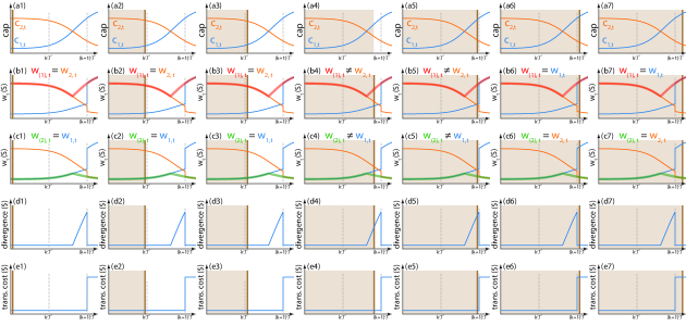
Figure 3: Schematic for the intraday rebalancing through rank switching of two stocks. Here, we examine a two-stock system and highlight the critical role of the rank switching. We consider two capitalization processes $c_{t,1}$ and $c_{t,2}$ that maintain their ranks during the rebalancing interval $((k-1)\mathcal{T},k\mathcal{T}]$ and switch their ranks during $(k\mathcal{T},(k+1)\mathcal{T}]$ (panel (a1-a7)). The red lines in panel (b1-b7) and green lines in panel (c1-c7) show the dollar-valued portfolio in rank space $w_{(1),\tau}$ and $w_{(2),\tau}$ respectively, where $w_{(k),t}$ denotes the dollar portfolio weights on the stock that occupies $k$-th rank in capitalization. The orange line in panel (b1-b7) and blue line in panel (c1-c7) show the dollar-valued portfolio in name space $w_{1,\tau}$ and $w_{2,\tau}$ respectively, where $w_{i,\tau}$ denotes the dollar portfolio weights on the stock that had $i$-th name index. We further calculate and present in panel (d1-d7) the divergence between the total dollar portfolio weights in rank space and in name space, defined as $w_{(1),t}+w_{(2),t}-w_{1,t}-w_{2,t}$. Panel (e1-e7) shows the cumulative cost from bid-ask spread arising from the active trading at the rebalancing point. We consider seven representative timestamps elaborated in section 2.3.2.

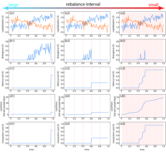
Figure 4: Transaction cost dependence on the rebalancing interval. This figure illustrates how transaction costs incurred by intraday rebalancing are influenced by different rebalancing intervals: large (panel (a1-e1)), medium (panel (a2-e2)), and small (panel (a1-a3)). The red vertical lines mark the rebalancing points across all panels. (a1-a3) The capitalization processes from two stocks. (b1-b3) The divergence between the total dollar portfolio weights in rank space and name space, $w_{(1),t}+w_{(2),t}-w_{1,t}+w_{2,t}$. The dollar portfolio weights in rank space $w_{(1),t},w_{(2),t}$, and in name space $w_{1,t},w_{2,t}$ are calculated based on capitalization processes in (a) following the intraday rebalancing strategy similar to Fig. 3. The maximum divergence decreases as rebalancing interval increases, aiding risk control. (c1-c3) The cumulative latency cost required to compensating divergences at the rebalancing points. Each point of rebalancing incurs a latency cost equal to the divergence between the total dollar portfolio weights in rank space and name space. (d1-d3) The cumulative cost from the bid-ask spread due to active trading at each rebalancing point. (e1-e3) The cumulative transaction cost. The cumulative transaction costs are the sum of latency costs and transaction costs. The medium rebalancing interval results in the lowest transaction costs while maintaining a manageable divergence, illustrating the importance of choosing an appropriate rebalancing interval.

2.4 Portfolio performance metrics

We evaluate the performance of various strategies by calculating the historical PnL and the derived portfolio metrics.

We define the value of the portfolio at time $t$ as $V_{t}$. For name space, we denote the normalized portfolio weights on the stock $i$ at day $t$ as $w_{i,t}^{R,\text{name}}$, subject to $l_{1}$-normalization condition $\sum_{i=1}^{N}|w_{i,t}^{R,\text{name}}|=1$. The corresponding PnL dynamics is given by

$$V_{t+1}=(1+r_{f,t+1})\times(V_{t}-\sum_{i}{\Lambda w_{i,t}V_{t}}-\text{T.C.})+\sum_{i}\Lambda V_{t}w_{i,t}(1+r_{i,t+1})\\$$ (2.4.1)

, where $\Lambda=1$ is the leverage, $r_{f,t+1}$ is the risk-free rate during the trading day $t+1$, and T.C. (transaction costs) are given by

$$\text{T.C.}=\eta\sum_{i}\Lambda|V_{t}w_{i,t}-V_{t-1}w_{i,t-1}(1+r_{i,t})|$$ (2.4.2)

. $\eta=0.0002$ is the transaction cost factor.

For rank space, we denote the normalized portfolio weights on rank $k$ at day $t$ as $w_{(k),t}^{R,\text{rank}}$, with $l_{1}$-normalization condition $\sum_{k=1}^{N}|w_{(k),t}^{R,\text{rank}}|=1$. Then, we calculate the corresponding PnL dynamics by adhering to the intraday rebalancing machinery introduced in section 2.3,

$$V_{t+1}= (V_{t}-\sum_{k=1}^{N}w_{(k),t}^{R,\text{rank}})(1+r_{f,t+1})+\sum_{k=1}^{N}\Lambda V_{t}w_{(k),t}^{R,\text{rank}}(1+\tilde{r}_{(k),t+1})$$ (2.4.3)

$$-\sum_{j:t<t+j\mathcal{T}\leq t+1}\text{cost}(t+j\mathcal{T}^{+};\Lambda V_{t}w_{(k),t}^{R,\text{rank}})$$

, where the $\text{cost}(t+j\mathcal{T}^{+};\Lambda V_{t}w_{(k),t}^{R,\text{rank}})$ is given in Eq. 2.3.6. In practice, this is achieved by the Algorithm 4.

The annualized return, volatility, and Sharpe ratio are straightforwardly derived from $V_{t}$ by

$$\begin{cases}r_{t_{i}}&=V_{t_{i}}/V_{t_{i}-1}-1,\quad\{t_{i}\}_{i=1}^{N}\in\text{ selected calendar year}\\ r_{\text{annual}}&=(\prod_{i=1}^{N}(1+r_{t_{i}}))^{252/N}\\ \sigma_{\text{annual}}&=\text{std}(\{r_{t_{i}}\}_{i=1}^{N})\\ \text{SR}_{\text{annual}}&=r_{\text{annual}}/\sigma_{\text{annual}}\end{cases}$$ (2.4.4)

, where $\{t_{i}\}_{i=1}^{N}$ are the daily timestamps within the selected calendar year to evaluate.

The practical implementation of the intraday rebalancing is summarized in Algorithm 5 along with a schematic in panel (g) in Fig. 5.

2.5 The statistical arbitrage algorithms

Here, we present the algorithms for the practical implementation of the formulation above. We also provide a schematic for the dependence of the algorithms in Fig. 5.

Input: $r_{t},r_{f,t},K$

Output: $\epsilon_{t},\Phi_{t}$

Function market_decomposition($r_{t},r_{f,t},K$):

      Principal component analysis: $r_{t}-r_{f,t}=U\Sigma V^{T}$

      $F_{t}\leftarrow(v_{1},v_{2},...,v_{K})$, where $v_{k}$ is the $k$-th column of $V^{T}$

      Calculate $\omega_{t}$ by solving $F_{t}=\omega_{t}(r_{t}-r_{f})$

      Calculate $\beta_{t}$ as the coefficient of the linear regression $r_{t}-r_{f}\sim F_{t}$

      $\Phi_{t}\leftarrow I-\beta_{t}\omega_{t}$

      $\epsilon_{t}\leftarrow\Phi_{t}(r_{t}-r_{f,t})$

     return $\epsilon_{t},\Phi_{t}$

// Input:

// $r_{t}$: return in name space or transformed return in rank space.

      // $r_{f,t}$: risk-free rate at the end of trading day $t$.

      // $K$: number of market factors, predetermined by analyzing eigenvalue

            // spectrum of the correlation matrix.

// Output:

// $\epsilon_{t}$: residual returns in name space or rank space.

// $\Phi_{t}$: transformation between residual space and equity space

      // (Eq. 2.1.1 for name space and Eq. 2.1.10 for rank space).

// Note:

      // The algorithm realizes the formulation in section 2.1.

      // Factors $F_{t}$ and $\omega_{t}$ are calculated on a 252-day look-back window.

      // Loadings $\beta_{t}$ are calculated on a 60-day look-back window.

      // $F_{t}$, $\omega_{t}$, and $\beta_{t}$ are updated daily.

      // $K=5$ for name space and $K=1$ for rank space based on empirical

      // eigenvalue spectrum of the correlation matrix (Fig. 6(c,d))).

Algorithm 1 Market decomposition (PCA) [Fig. 5, panel(c1, c2)]

Input: $\epsilon_{t},\Phi_{t}$

Output: $w_{t}^{R|\text{OU}}$

Function portfolio_weights_by_parametric_model($\epsilon_{t},\Phi_{t})$

      Calculate $x_{t}^{L}$ by Eq. 2.2.1

      Estimate $\tau,\mu,\sigma,x_{t},R^{2}$ by fitting $x_{t}^{L}$ to an OU process (Eq. 2.2.4)

      Calculate $w_{t}^{\epsilon|\text{OU}}$ by Eq. 2.2.7

      $w_{t}^{R|\text{OU}}\leftarrow\Phi_{t}^{T}w_{t}^{\epsilon|\text{OU}}$(Eq. 2.2.10)

      return $w_{t}^{R|\text{OU}}/||w_{t}^{R|\text{OU}}||_{1}$

// Input:

// $\epsilon_{t}$: residual returns calculated from Algorithm 1

// $\Phi_{t}$: transformation matrix between equity space and residual space from

      // Algorithm 1

// Output:

// $w_{t}^{R|\text{OU}}$: $l_{1}$-normalized portfolio weights by parametric model.

            // For name space, it stands for the portfolio weights on stocks.

            // For rank space, it corresponds to the portfolio weights on

            // artificial financial instruments that realize rank returns

            // defined in Eq. 2.1.9.

// Note:

      // The algorithm realizes the formulation in section 2.2.1.

      // $\tau$, $\mu$, $\sigma$ are fitting parameters of OU process.

      // Risk control by ignoring $\tau>30$ days (Eq. 2.2.7).

Algorithm 2 Portfolio weights by parametric model [Fig. 5, panel(d1, e1)]

Input: $\epsilon_{t},\Phi_{t}$

Output: $w_{t}^{R|\text{NN}}$

Function portfolio_weights_by_neural_networks($\epsilon_{t},\Phi_{t})$

      Calculate $x_{t}^{L}$ by Eq. 2.2.1

      if name space

            Train neural network in-sample for mean-variance optimization (Eq. 2.2.13)

      if rank space

            Train neural network in-sample for mean-variance optimization (Eq. 2.2.14)

      Calculate $w_{t}^{\epsilon|\text{NN}}$ out-of-sample from trained neural network

      return $w_{t}^{R|\text{NN}}/||w_{t}^{R|\text{NN}}||_{1}$

// Input:

// $\epsilon_{t}$: residual returns calculated from Algorithm 1.

// $\Phi_{t}$: transformation matrix between equity space and residual space from

      // Algorithm 1.

// Output:

// $w_{t}^{R|\text{NN}}$: $l_{1}$-normalized portfolio weights by parametric model.

            // For name space, it stands for the portfolio weights on stocks.

            // For rank space, it corresponds to the portfolio weights on

            // artificial financial instruments that realize rank returns.

            // defined in Eq. 2.1.9.

// Note:

      // The algorithm realizes the formulation in section 2.2.2.

      // No pre-screening on trading opportunities $x_{t}^{L}$ applied.

      // Neural networks internally prioritize various trading opportunities

            // and manage risk (Fig. 10, Fig. 11).

      // The mean-variance target is evaluated on a 24-day window.

Algorithm 3 Portfolio weights by neural networks [Fig. 5, panel(d2, e2)]

Input: $w_{t}^{R},r_{f,t},\mathcal{T}$

            $c_{t+\tau},\quad t=1,2,...,T$ (days), $\tau=1,2,...,N$ (minutes)

Output: $V_{t},\quad t=1,2,...,T+1$

Function intraday_rebalancing($w_{t}^{R},r_{f,t},\mathcal{T},c_{t+\tau})$

      $t\leftarrow 0$, $V_{t}\leftarrow 1$, $w^{\text{prev}}\leftarrow 0$

      While $t\leq T$ $\triangleright$ $T$ is daily time tick

            $w_{(k),t}^{\text{rank}}\leftarrow w_{(k),t}^{R},\quad k=1,2,...,N$

            $w_{\mathcal{I}_{(k),t},t}^{\text{name}}\leftarrow w_{(k),t}^{R},\quad k=1,2,...,N$ $\triangleright$ $\mathcal{I}_{(k),t}$ maps from rank to name

            $V_{t}\leftarrow V_{t}-\sum_{i}w_{i,t}^{\text{name}}-0.0002\times||w_{t}^{\text{name}}-w^{\text{prev}}||_{1}$

            $\tau\leftarrow 0$

            While $t+\tau<(t+1)$ $\triangleright$ $\tau$ is intraday time tick

                  $w_{(k),t+\tau}^{\text{rank}}\leftarrow w_{(k),t+\tau-1}^{\text{rank}}\times\frac{c_{(k),t+\tau}}{c_{(k),t+\tau-1}},k=1,2,...,N$ (Eq. 2.3.4)

                  $w_{i,t+\tau}^{\text{name}}\leftarrow w_{i,t+\tau-1}^{\text{name}}\times\frac{c_{i,t+\tau}}{c_{i,t+\tau-1}},i=1,2,...,N$ (Eq. 2.3.5)

                  $\triangleright$ $t+\tau-1$ and $t+\tau$ are adjacent intraday timestamps

                  if $\tau\%\mathcal{T}==0$ or end of the trading day $\triangleright$ rebalancing point

                        Calculate $\text{cost}(t+\tau,w_{(k),t}^{\text{rank}})$ by Eq. 2.3.6

                        $V_{t}\leftarrow V_{t}-\text{cost}(t+\tau,w_{(k),t}^{\text{rank}})$

                        $w_{\mathcal{I}_{(k),t+\tau},t+\tau}^{\text{name}}\leftarrow w_{(k),t+\tau}^{\text{rank}},\quad k=1,2,...,N$

                  $\tau\leftarrow\tau+1$

            $V_{t+1}\leftarrow(1+r_{f,t+1})V_{t}+\sum_{i}w_{i,t+\tau}^{\text{name}}$

            $w^{\text{prev}}\leftarrow w_{t+\tau}^{\text{name}}$

            $t\leftarrow t+1$

      return $V_{t},\quad t=1,2,...,T+1$

// Input:

      // $w_{t}^{R}$: the $l_{1}$-normalized portfolio weights from either parametric

            // model (Algorithm 2) or neural networks (Algorithm 3).

// $r_{f,t}$: risk-free rate during the trading day $t$.

// $\mathcal{T}$: rebalance interval.

// $c_{t+\tau}$: the capitalization processes in name space and rank space at

                  // 1-minute resolution throughout the trading day $t$.

                  // $t$ is the time tick at daily level.

                  // $\tau$ is the time tick at minute level.

// Output:

      // $V_{t}$: the value process of the portfolio (PnL) with weights $w_{t}^{R}$.

// Note:

      // The algorithm realizes the formulation in section 2.3.1.

      // In essence, it converts portfolio weights from rank to name

            // at $\mathcal{T}$ minutes interval.

Algorithm 4 intraday rebalancing [Fig. 5, panel (f3)]

Input: $V_{t},\quad t=1,2,...,N$

Output: $r_{\text{annual}}$, $\sigma_{\text{annual}}$, $\text{SR}_{\text{annual}}$

Function portfolio_metric($V_{t},r_{f}$)

      For year in years_in_backtesting:

            Locate all $t_{1}\leq t_{2}\leq...\leq t_{N}$ in year

            $r_{t_{i}}=V_{t_{i}}/V_{t_{i-1}}-1,\quad i=1,2,...,N$

            $r_{\text{annual}}\leftarrow(\prod_{i=1}^{N}(1+r_{t_{i}}))^{252/N}-1$

            $\sigma_{\text{annual}}\leftarrow\sqrt{252}\times\text{std}(\{r_{t_{i}}\}_{i=1}^{N})$$\triangleright$ std is the standard deviation

            $\text{SR}_{\text{annual}}\leftarrow(r_{\text{annual}}-r_{f,\text{annual}})/\sigma_{\text{annual}}$ $\triangleright$ $r_{f,\text{annual}}$ is annualized risk-free rate

      return $r_{\text{annual}},\sigma_{\text{annual}},\text{SR}_{\text{annual}}$ for all backtesting years

// Input:

// $V_{t}$: the value process (PnL) of the portfolio with weights $w_{t}^{R}$.

      // $r_{f,t}$: the risk-free rate at the end of trading day $t$.

// Output:

// The algorithm realizes the formulation in section 2.4.

// $r_{\text{annual}}$: the annualized return for all backtesting years.

// $\sigma_{\text{annual}}$: the annualized volatility for all backtesting years.

// $\text{SR}_{\text{annual}}$: the Sharpe ratio for all backtesting years.

Algorithm 5 portfolio metric [Fig. 5, panel (g)]

Input: $r_{t},r_{f},K$

Called algorithm: Algorithm 1, Algorithm 2, Algorithm 3, Algorithm 5

Output: $w_{t}^{R},V_{t}$, $\text{SR}_{\text{annual}}$

Function statistical_arbitrage_in_name_space($r_{t},r_{f,t},K)$

      $\epsilon_{t},\Phi_{t}\leftarrow\text{market\_decomposition}(r_{t},r_{f,t},K)$ from Algorithm 1

      if parametric model

            $w_{t}^{R|\text{OU}}\leftarrow\text{portfolio\_weights\_by\_parametric\_model}(\epsilon_{t},\Phi_{t})$ from Algorithm 2;

      if neural networks

            $w_{t}^{R|\text{NN}}\leftarrow\text{portfolio\_weights\_by\_neural\_network}(\epsilon_{t},\Phi_{t})$ from Algorithm 3

      Calculate PnL $V_{t}$ by Eq. 2.4.1

      $r_{\text{annual}}$, $\sigma_{\text{annual}}$, $\text{SR}_{\text{annual}}\leftarrow$ portfolio_metric($V_{t},r_{f,t}$) from Algorithm 5

      return $w_{t}^{R},V_{t}$, $\text{SR}_{\text{annual}}$

// Input:

// $r_{t}$: dividend-adjusted daily return in name space.

      // $r_{f,t}$: risk-free rate at the end of trading day $t$.

      // $K$: number of market factors, predetermined by analyzing eigenvalue

            // spectrum of the correlation matrix.

// Output:

// $w_{t}^{R}$: the $l_{1}$-normalized portfolio weights on stock.

// $V_{t}$: the value process (PnL) of the portfolio with weights $w_{t}^{R}$.

// $r_{\text{annual}}$, $\sigma_{\text{annual}}$, $\text{SR}_{\text{annual}}$: annualized return, volatility, and Sharpe

                                                   // ratio.

Algorithm 6 (Integrated) Statistical arbitrage in name space

Input: $c_{t},c_{t+\tau},r_{f},K$

Called algorithm: Algorithm 1, Algorithm 2, Algorithm 3, Algorithm 4, Algorithm 5

Output: $w_{t}^{R},V_{t}$, $r_{\text{annual}}$, $\sigma_{\text{annual}}$, $\text{SR}_{\text{annual}}$

Function statistical_arbitrage_in_name_space($c_{t},r_{f,t},K)$

      Calculate $\tilde{r}_{t}$ by Eq. 2.1.9

      $\tilde{\epsilon}_{t},\tilde{\Phi}_{t}\leftarrow\text{market\_decomposition}(\tilde{r}_{t},r_{f,t},K)$ from Algorithm 1

      if parametric model

            $w_{t}^{R|\text{OU}}\leftarrow\text{portfolio\_weights\_by\_parametric\_model}(\epsilon_{t},\Phi_{t})$ from Algorithm 2;

      if neural networks

            $w_{t}^{R|\text{NN}}\leftarrow\text{portfolio\_weights\_by\_neural\_network}(\epsilon_{t},\Phi_{t})$ from Algorithm 3

      $V_{t}\leftarrow$ intraday_rebalancing($w_{t}^{R|\text{NN}},r_{f,t},\mathcal{T},c_{t+\tau}$) from Algorithm 4

      $r_{\text{annual}}$, $\sigma_{\text{annual}}$, $\text{SR}_{\text{annual}}\leftarrow$ portfolio_metric($V_{t},r_{f,t}$) from Algorithm 5

      return $w_{t}^{R},V_{t}$, $r_{\text{annual}}$, $\sigma_{\text{annual}}$, $\text{SR}_{\text{annual}}$

// Input:

// $c_{t}$: capitalizations at the end of trading day $t$.

// $c_{t+\tau}$: capitalization process at 1-minute resolution throughout the

                  // trading day $t$. $t$ is the time tick at daily level.

                  // $\tau$ is the time tick at intraday level.

      // $r_{f,t}$: risk-free rate at the end of trading day $t$.

      // $K$: number of market factors, predetermined by analyzing eigenvalue

            // spectrum of the correlation matrix.

// Output:

      // $w_{t}^{R}$: the $l_{1}$-normalized portfolio weights on artificial financial

            // instruments that realize $\tilde{r}_{t}$.

      // $V_{t}$: the value process (PnL) of the portfolio with weights $w_{t}^{R}$.

      // $r_{\text{annual}}$, $\sigma_{\text{annual}}$, $\text{SR}_{\text{annual}}$: annualized return, volatility, and Sharpe

                                                   // ratio.

Algorithm 7 (Integrated) Statistical arbitrage in rank space

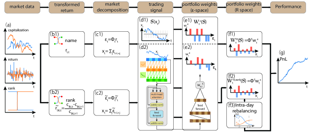
Figure 5: Schematic of the statistical arbitrage algorithm in name space and rank space. Our framework encompasses seven core components (from left to right), (1) market data, (2) transformed return, (3) market decomposition, (4) trading signal, (5) portfolio weights in residual space (denoted as $\epsilon$-space), (6) portfolio weights in equity space (denoted as $R$-space), and (7) portfolio performance. A high-level summary is discussed in section 2.5. (a) Market data. The market data consists of (i) dividend-adjusted daily return for name space in section 2.1.1 and (ii) capitalization and rank in capitalization for rank space in section 2.1.2. (b1, b2) Transformed return. The raw dividend-adjusted return in name space as inputs for statistical arbitrage in name space (b1) and the rank return in continuous time limit as inputs for statistical arbitrage in rank space (b2). (c1-c2) Market decomposition. The market decomposition is elaborated for name space in section 2.1.1 and for rank space in section 2.1.2. (d1-d2, e1-e2, f1-f2) Trading signal and portfolio weights. The trading signals and portfolio weights in residual space for both name and rank space are elaborated in section 2.2, with a parametric model in section 2.2.1 (d1, e1) and deep neural networks in section 2.2.2 (d2, e2). Panel (d1) is a schematic drawing for trading strategy dictated by the parametric model. The corresponding portfolio weights $w_{t}^{\epsilon|\text{OU},\text{name/rank}}$ are shown in panel (e1), where the portfolio takes a uniform leverage across all trading opportunities. Panel (d2, e2) is a schematic drawing for the architecture of our deep neural network, with a two-layer convolutional neural network followed by a one-layer transformer encoder and a feed-forward network. The corresponding portfolio weights $w_{t}^{\epsilon|\text{NN}}$ are shown in panel (e2), where leverages for different trading opportunities differ. The portfolio weights in equity space are calculated from the portfolio weights in residual space, as discussed in section 2.2.1 and 2.2.2 for both name space (f1) and rank space (f2). (f3) Intraday rebalancing. The portfolio in (f2) is realized by intraday rebalancing to overcome the realizability issue with rank return, as elaborated in section 2.3. (g) Portfolio performance. The historical PnL is calculated to measure the performance of different strategies.

3 Empirical results for the U.S. equities

This section presents empirical results for the U.S. equities and demonstrates the improved performance of statistical arbitrage in rank space compared to name space. In section 3.1, we detail our data sources and numerical experiments. Sections 3.2 and 3.3 provide an in-depth comparison of market structure and residual return characteristics between name space and rank space. It reveals a single-factor-driven market in rank space and a more robust mean-reversion of residual returns in rank space, the main motivations for operating statistical arbitrage in rank space. In section 3.4, we systematically present the portfolio performance in rank space. We show that the portfolios constructed by the parametric OU model and neural networks in rank space significantly outperform their counterparts in name space when transaction costs are excluded. However, portfolio performance in rank space diminishes rapidly with transaction costs due to substantial costs from intraday rebalancing. Nevertheless, the portfolios calculated by neural networks in rank space achieve an average annual return of 35.68% and an average Sharpe ratio of 3.28 from 2007 to 2022, whereas the portfolios by the parametric OU model in rank space cease to profit. To understand the difference in portfolio performance between the parametric OU model and the neural networks, section 3.5 analyzes the intelligent trading strategy by neural networks, characterized by flexible leverages and reduced holding time. Section 3.6 discusses the relationship between the optimal intraday rebalancing interval and the characteristic time of rank switching. Section 3.7 examines the dependence of portfolio performance on transaction cost and dollar neutrality.

3.1 Data and experimental setup

We collect dividend-adjusted daily return, price, numbers of shares outstanding, and capitalizations for the US securities on CRSP from January 1990 to December 2022. We also collect the intraday price data at 1-minute resolution from Polygon.io from January 2005 to December 2022. We further derived the capitalization data at 1-minute resolution by combining the numbers of shares outstanding from CRSP and intraday price data from Polygon.io. We use the one-month Treasury bill rates from the Kenneth French Data Library as the risk-free rate $r_{f}$.

Our backtesting starts from January 2006 to December 2022, including the subprime mortgage crisis period and the years after 2010 when conventional statistical arbitrage has become much more competitive and less profitable. On each trading day after the market close, we re-calibrate our investment universe and select stocks that (i) rank top 500 in capitalizations at day $t$ to ensure enough liquidity and (ii) have valid historical return data at day $t+1$. This minimizes the potential selection bias to our best efforts. We further carry out PCA on the selected returns with a 252-day lookback window and extract leading eigenvectors for market factors. Specifically, we choose the five eigenvectors associated with the top five eigenvalues in the name space and one eigenvector associated with the top eigenvalue in the rank space. The factor loadings $\beta_{t}$ are calculated on a 60-day lookback window, from which we calculate the $\Phi_{t}$ and $\epsilon_{t}$. The cumulative residual returns $x_{t}^{L}$ are evaluated on the same 60-day lookback window, and fed into either the parametric model or deep neural networks to calculate the portfolio weights and PnL. The procedure is carried out in both name and rank space.

The neural networks are trained in two steps. The first step aims at optimizing the hyper-parameters of neural network. Specifically, to evaluate the portfolio weights from the trading day $t$ to day $t+252$, we utilize the data from $t-1000$ to $t-60$ as the training data set and from $t-59$ to $t-1$ as the validation data set, from which we determine hyper-parameters from the converged mean-variance target in the training curve (Fig. 12). The hyperparameters of our optimized neural network architecture are elaborated in section 2.2.2.

The second step aims at increasing the updating frequency of parameters in the neural networks from annually to quarterly while keeping hyper-parameters fixed. More explicitly, to evaluate the portfolio weights from the trading day $t$ to day $t+63$, we use the data from trading day $t-500$ to day $t-1$ as the training data set. Empirically, increasing the updating frequency is significantly beneficial to the performance of neural network, due to the non-stationarity in financial data. The training tasks utilize PyTorch 2.2.0, and are parallelized on a workstation with a CPU from AMD Ryzen Threadripper Pro 5955 WX and two GPUs from Nvidia GeForce RTX 4090. The entire training process takes two days to complete for both name space and rank space.

3.2 Market structure: name space versus rank space

We initiate our discussion by presenting a robust market structure in rank space, the main motivation for our adventure on statistical arbitrage in rank space. We show the proportion of the market capitalization as a function of ranks in capitalization averaged over a series of 5-year periods from 1991 to 2022 in Fig. 6(a)[11]. The distribution of the capitalizations across different ranks remains stable throughout the history considered, despite varying macro- and micro-economic conditions for each individual stock in name space. This indicates that a robust representation could emerge for the market in rank space. A more detailed PCA on the correlation matrix features a much enhanced leading eigenvalue in rank space compared to that in name space (Fig. 6(b)). The enhanced first eigenvalue in rank space highlights more variances explained by the first eigenvector in rank space compared to that in name space, pointing to a more structured market in rank space.

More importantly, the single-factor-driven market in rank space significantly facilitates the market decomposition. To demonstrate, we present the empirical probability distribution of the eigenvalue spectra of the correlation matrix calculated from the market in both name and rank space in Fig. 6(c1-c6) and (d1-d6), respectively. The eigenvalue spectra for the market in name space does not merit a sharp bulk-edge separation, with several eigenvalues lying above the Marchenko-Pastur upper bound[2] (Fig. 6(c1-c6)), indicating a multi-factor driven market in name space. While considerable efforts from both theoretical and empirical aspects have been made for a bulk-edge separation and interpret the leading eigenportfolios[2, 14], the ambiguity remains for identifying market factors. In sharp contrast, the market in rank space is driven by a single factor, as evidenced by a clear bulk-edge separation in Fig. 6(d1-d6). The single-factor-driven market in rank space clears out most ambiguity for separating market factors and residuals in the market decomposition. Therefore, we choose the first five eigenvectors as market factors in name space ($K=5$), and the leading eigenvector as the single factor in rank space ($K=1$) for our market decomposition (Algorithm 1).

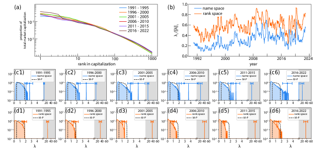
Figure 6: Market structure in name space versus rank space. (a) Proportion of total market capitalization versus ranks in capitalization. The proportion of market capitalization is averaged over a series of 5-year interval from 1991 to 2022. (b) The principal eigenvalue of the correlation matrices of $r_{t}$ in name space (blue) and for $\tilde{r}_{t}$ rank space (orange). The correlation matrices, including the top 500 stocks in capitalization, are calculated on a 60-day lookback window, and updated every 10 days. A consistently higher first eigenvalue in rank space compared to name space suggests that a larger variance is explained by the leading eigenvector in rank space, indicating a more structured market. (c,d) The empirical probability distribution density of the eigenvalue spectrum of the correlation matrices versus Marchenko-Pastur distribution. The correlation spectrum is updated every 10 days with a lookback window of 60 days over a 5-year period, yielding $\sim 125$ eigenvalue spectra for the correlation matrix every 5 years. The empirical distribution from the first three eigenvalues is represented by a single spike located at the average of the corresponding eigenvalue, with an error bar indicating their temporal standard derivation. The $x$-axis is split into two segments per sub-panel for clarity: the left half ranges from 0 to 5, and the right half ranges from 5 to 50, emphasized by a shaded background for the right half range. The black-dashed lines depict the Marchenko-Pastur distribution with $\lambda:=T/N=60/500$. The need for multiple eigenvectors (factors) in name space is evident as several eigenvalues lie near or above the Marchenko-Pastur upper bound (c1-c6), contrasting sharply with the rank space, where a distinct bulk-edge separation exists. This suggests a market predominantly driven by a single factor in rank space.

3.3 Robust mean-reversion of residual returns in rank space

While the single-factor-driven market in rank space facilitates market decomposition, the performance of statistical arbitrage ultimately hinges on the mean-reversion of residual returns. Here, we report a markedly enhanced mean-reverting behavior for residual returns in rank space compared to name space, laying the foundation for superior performance of statistical arbitrage in rank space.

We employ two measures to quantify mean-reversion, (i) the mean-reversion time parametrized by fitting the cumulative residual returns to the OU process and (ii) the empirical distribution of the cumulative residual returns referenced by standard Brownian motion. For the first measure, we systematically fit the cumulative residual return $x_{t}^{L}$ to the OU process and determine the mean-reverting time $\tau$. We evaluate the empirical distribution of $\tau$ over a five-year period from 1991 to 2022 for both name space (Fig. 7(a1-a6)) and rank space (Fig. 7(b1-b6)). A shaded area highlights the slow mean-reverting regime ($\tau>30$ days), the less favorable regime for statistical arbitrage. The distribution of $\tau$ in rank space is more concentrated in the fast mean-reverting regime, starkly contrasting the heavy-tailed distribution towards large $\tau$ in name space. This faster mean-reverting time in rank space substantiates its superiority.

Additionally, the superior mean-reverting behavior in rank space is further demonstrated by comparing the empirical distribution of normalized cumulative residual returns, $\tilde{x}_{t}^{L}$ calculated from name space and rank space. We define the normalized cumulative residual returns as follows:

$$\hat{x}_{t}^{L}=(\hat{x}_{t-L+1},\hat{x}_{t-L+2},...,\hat{x}_{t}),\quad\text{where }\hat{x}_{t-L+\alpha}=\frac{1}{{\hat{\sigma}_{t}^{L}}\sqrt{\alpha}}\sum_{j=1}^{\alpha}\epsilon_{t-L+j}$$ (3.3.1)

, where $\hat{\sigma}_{t}^{L}$ is the estimated standard deviation of $\{\epsilon_{t-L+j}\}_{j=1}^{L}$. Suppose the residual returns follow uncorrelated, normal distribution, i.e. $\{\epsilon_{t-L+j}\}_{j=1}^{L}\sim\mathcal{N}(\boldsymbol{0},\boldsymbol{I}_{L})$, the derived cumulative residual returns $x_{t}^{L}$ will follow a standard Brownian motion and the normalized cumulative residual return defined in Eq. 3.3.1 will be normally distributed, i.e. $\hat{x}_{t-L+\alpha}\sim\mathcal{N}(0,1)$, $\forall\alpha=1,2,...L$. Consequently, it will serve as a measure of mean-reversion of the difference in probability density function (p.d.f.) between the empirical observations on market and the normal distribution,

$$\text{p.d.f.}(\hat{x}_{t-L+\alpha})-\frac{1}{\sqrt{2\pi}}\exp(-\frac{\hat{x}_{t-L+\alpha}^{2}}{2}),\quad\alpha=1,2,...,L$$ (3.3.2)

The difference is accessed over a series of five-year periods from 1991 to 2022 for both name space (Fig. 8(a1-a6)) and rank space (Fig. 8(b1-b6)). A more concentrated distribution of $\hat{x}_{t-L+\alpha}$ than Brownian motion indicates good mean-reverting behavior, especially for large $\alpha$. This is particularly evident in rank space, where a robust dominance of red color in the heatmaps for large $\alpha$ regime (highlighted in dashed boxes in Fig. 8) underscores the concentrated nature of $\hat{x}_{t}^{L}$ in rank space. Such behavior provides critical evidence of a more robust mean-reversion of residual returns in rank space. In stark contrast, the similar dominance by red color in name space was evident in 1990s (Fig. 8(a1, a2)), but progressively deteriorated since 2000s (Fig. 8(a5-a6)), and finally disappears after 2010s (Fig. 8(a5-a6)). This marks the deterioration of the mean-reversion of $x_{t}^{L}$ in name space after the 2010s, echoing the failure of profiting from conventional statistical arbitrage strategies after 2010s.

In summary, our analysis demonstrates that the rank space exhibits more robust mean-reverting behavior compared to name space, as evidenced by a detailed examination of the mean-reverting time and the distribution of cumulative residual returns.

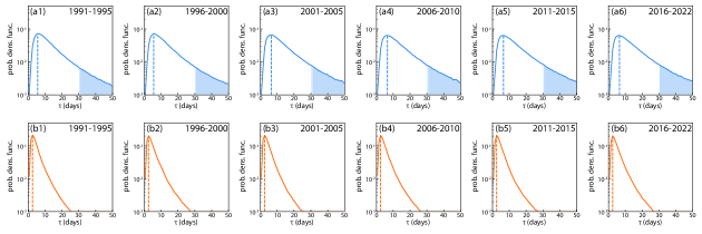
Figure 7: Mean-reverting time in name space versus rank space. We evaluate the empirical distributions of the mean-reverting time $\tau$ in name space across a series of five-year periods from 1991 to 2022. The $\tau$ is evaluated by fitting the cumulative residual return $x_{t}^{L}$ to an Ornstein–Uhlenbeck(OU) process. (a1-a6) The empirical distributions of $\tau$ in name space, with maximum empirical probability at $\sim 6$ days (vertical dashed lines). The relatively long mean-reverting times ($\tau>30$ days) highlighted in shaded areas are prevalent, which is less favorable conditions for statistical arbitrage. (b1-b6) The empirical distributions of the mean-reverting time $\tau$ in rank space, with maximum empirical probability at $\sim 2.5$ days (vertical dashed lines). Instances of $\tau>30$ days are almost negligible, demonstrating a more pronounced mean-reversion behavior, more favorable for statistical arbitrage.

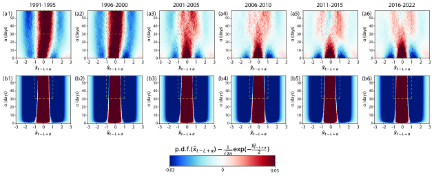
Figure 8: Empirical distributions of normalized cumulative residual returns: name space versus rank space. The cumulative residual returns $x_{t}^{L}$ are normalized according to Eq. 3.3.1. This normalization facilitates the conversion of comparisons between trajectories of $x_{t}^{L}$ and Brownian motion into comparisons of the probability density of the empirical distribution of $\hat{x}_{t}^{L}$ against the normal distribution. Consequently, we present the difference between the empirical probability density of $\hat{x}_{t}^{L}$ and standard normal distribution. The empirical probability density of $\hat{x}_{t}^{L}$ is evaluated across a series of five-year periods from 1991 (left) to 2022 (right) in both (a1-a6) name space and (b1-b6) rank space. The dashed brown box highlights the critical regime where a dominating red color indicates a more concentrated distribution of $x_{t-L+\alpha}$ for large $\alpha$. This concentration signals superior mean-reversion capabilities, particularly evident in rank space throughout the last thirty years. Furthermore, the distribution of $\hat{x}_{t}^{L}$ in name space evolves significantly, indicating a progressively deteriorating mean-reversion in name space after 2010. This echoes the relatively poor performance in our backtesting. The stark contrast in $\hat{x}_{t}^{L}$ supports the strategic advantage of operating in rank space for statistical arbitrage.

3.4 Portfolio performance

In this section, we systematically present the dynamics of PnL $V_{t}$ in Fig. 9. We compute $V_{t}$ by Eq. 2.4.1 in name space and by Eq. 2.4.3 in rank space where the portfolio weights $w_{t}^{R}$ are calculated by four scenarios: (i) the parametric model in name space in panel (a), (ii) the parametric model in rank space in panels (b,c), (iii) neural networks in name space in panel (d), and (iv) neural networks in rank space in panels (e, f). In Fig. 9(g,h), we summarize the averaged Sharpe ratio from 2016 to 2022 for each scenario, supplemented by year-over-year summary statistics without transaction costs in Table 1 and with transaction costs in Table 2.

As expected, the traditional statistical arbitrage in name space yields diminishing profits post-2010s, echoing deteriorated mean-reversion in Fig. 8(a1-a6). On the other hand, the statistical arbitrage with a parametric model in rank space produces mixed bitter-sweet results. On the positive side, due to enhanced mean-reversion, the PnL and Sharpe ratio in rank space initially show tempting performances without transaction costs (Fig. 9(b)). This scenario assumes rank returns in continuous-time limit $\tilde{r}_{t}$ are realized without penalty, representing an ideal situation free from bid-ask spread ($\eta=0$) and continuous intraday rebalancing ($\mathcal{T}\rightarrow 0$). However, after accounting for real transaction costs ($\eta=0.0002$) with finite rebalancing interval ($\mathcal{T}=225$ minutes), the PnL exhibits a monotonic decline (Fig. 9(c)) with unfavorable Sharpe ratios (Fig. 9(h)). This stark contrast underscores the significant expenses associated with realizing rank returns in continuous time limit $\tilde{r}_{t}$.

Improvements can be pursued from at least two angles. First, we can leverage the intelligence of neural networks to better exploit the enhanced mean-reversion in rank space, potentially further boosting profits to offset transaction costs. Second, we may develope better methods to ”trade ranks” that minimize the costs associated with realizing $\tilde{r}_{t}$, compared to those incurred from intraday rebalancing here. Here, we focus on the first direction, reserving the exploration of the second for subsequent research works.

The application of neural networks in both name space and rank space demonstrated divergent outcomes. In name space, neural networks do not enhance performance in terms of return or Sharpe ratio (Fig. 9(a, d), Table 1, and Table 2). Conversely, in rank space, neural networks significantly improve the PnL (Fig. 9(e, f)), achieving an average annual return of 35.68% and an average Sharpe ratio of 3.28 from 2007 to 2022 (Fig. 9(h), Table 2). This success is driven by the effective exploitation of mean-reversion behavior in rank space by neural networks that yields an average annual return of 206.49% and an average annual Sharpe ratio of 9.04 without transaction costs (Fig. 9(g), Table 1) – sufficient to offset the substantial costs in intraday rebalancing to realize $\tilde{r}_{t}$.

In addition, we observe a consistent increase in the volatility of portfolios in rank space compared to those in name space, regardless of whether the parametric OU model or neural networks are used or whether the transaction costs are included. To investigate the cause of this increased volatility, we analyze the average holding time of active positions in residual space for both name space and rank space, as shown in Fig. 11. The results indicate that portfolios in rank space have a significantly shorter holding time than those in name space, which contributes to the higher portfolio volatility.

In summary, benefited from the robust mean-reversion of residual returns in rank space and the intelligence of neural networks, we demonstrate the superior portfolio performance by statistical arbitrage in rank space. Our results also highlight the transaction costs associated with the realizing rank returns in the continuous time limit, which pose the main challenge for the arbitrage strategies in rank space.

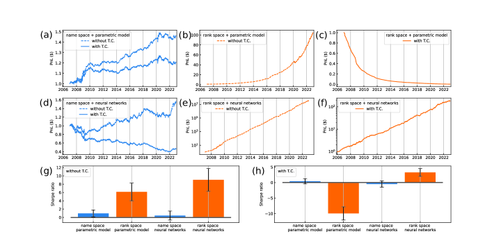
Figure 9: Summary of portfolio performance. The PnL dynamics $V_{t}$ are calculated according to Eq. 2.4.1 in name space and Eq. 2.4.3 in rank space. (a) The PnL using portfolio weights derived from the parametric model in name space. The solid (dashed) line shows the PnL with (without) transaction costs. (b, c) The PnL using portfolio weights derived from the parametric model in rank space. The dashed line shows the PnL without transaction costs in panel (b) and the solid line shows the PnL with transaction costs in panel (c). (d) The PnL using portfolio weights derived from the neural networks in name space. The solid (dashed) line shows the PnL with (without) transaction costs. (e, f) The PnL using portfolio weights derived from the neural networks in rank space. The dashed line shows the PnL without transaction costs in panel (e) and the solid line shows the PnL with transaction costs in panel (f). The y-axes are in log-scale in panel (e,f), different from the linear scale in other panels. (g, h) The average Sharpe ratio for different scenarios without transaction costs in panel (g) and with transaction costs in panel (h). The error bars indicate the temporal standard deviation of the Sharpe ratio from 2006 to 2022. Annualized returns, volatilities, and Sharpe ratios for each calendar year are calculated by Algorithm 5 and detailed in Table 1 without transaction costs and in Table 2 with transaction costs. We choose 2 basis points for our transaction costs.

year	Name space parametric model			rank space parametric model			name space neural networks			rank space neural networks
	return	vol	SR	return	vol	SR	return	vol	SR	return	vol	SR
2007	2.87%	0.02	1.38	8.52%	0.04	1.90	-8.37%	0.10	-0.87	79.41%	0.14	5.62
2008	7.42%	0.04	1.70	25.44%	0.06	3.96	-6.98%	0.13	-0.52	239.88%	0.38	6.36
2009	7.01%	0.03	2.02	27.81%	0.08	3.57	3.91%	0.13	0.29	414.09%	0.35	11.72
2010	-0.49%	0.02	-0.24	31.73%	0.05	6.21	-0.02%	0.08	0.00	222.37%	0.19	11.41
2011	1.91%	0.02	0.85	40.14%	0.06	7.12	12.84%	0.08	1.67	126.84%	0.22	5.76
2012	-0.40%	0.02	-0.22	41.06%	0.05	8.20	7.35%	0.07	1.00	162.37%	0.20	8.20
2013	1.19%	0.02	0.70	27.92%	0.05	5.74	8.34%	0.07	1.14	289.73%	0.21	13.96
2014	3.65%	0.02	2.07	43.82%	0.05	8.84	-3.24%	0.07	-0.49	168.89%	0.14	12.07
2015	0.81%	0.02	0.41	41.78%	0.06	7.44	0.71%	0.08	0.09	137.95%	0.19	7.10
2016	2.79%	0.02	1.43	61.86%	0.07	9.51	8.58%	0.10	0.90	293.85%	0.27	11.02
2017	1.56%	0.02	0.93	30.58%	0.04	7.04	9.88%	0.07	1.35	208.30%	0.17	12.10
2018	3.07%	0.02	1.44	27.78%	0.05	5.71	3.67%	0.06	0.60	151.91%	0.19	7.83
2019	4.50%	0.02	2.44	41.42%	0.05	8.39	-6.84%	0.06	-1.07	175.91%	0.20	8.59
2020	1.56%	0.04	0.39	25.06%	0.09	2.89	1.24%	0.09	0.14	307.81%	0.28	10.84
2021	-0.67%	0.02	-0.28	37.60%	0.06	6.21	-2.32%	0.08	-0.30	177.60%	0.25	7.11
2022	1.05%	0.03	0.36	36.79%	0.07	5.53	28.84%	0.09	3.29	146.86%	0.29	5.00
Avg	2.36%	0.02	0.96	34.33%	0.06	6.14	3.60%	0.08	0.45	206.49%	0.23	9.04

Table 1: Portfolio performance without transaction costs. The portfolios in rank space consistently outperform their counterparts in name space, both with the parametric model and neural networks. The neural networks improve the portfolio performance in rank space dramatically, in stark contrast with negligible improvements in name space. The contrast echoes with the fact that the neural networks are much more effective in rank space compared to that in name space Fig. 12.

year	Name space parametric model			rank space parametric model			name space neural networks			rank space neural networks
	return	vol	SR	return	vol	SR	return	vol	SR	return	vol	SR
2007	1.63%	0.02	0.79	-32.51%	0.04	-7.67	-15.51%	0.10	-1.61	26.07%	0.10	2.55
2008	6.02%	0.04	1.38	-43.78%	0.05	-9.58	-14.19%	0.13	-1.06	36.40%	0.18	2.04
2009	5.71%	0.03	1.65	-32.78%	0.04	-8.07	-3.13%	0.13	-0.23	48.97%	0.13	3.67
2010	-1.69%	0.02	-0.82	-32.83%	0.03	-12.68	-7.25%	0.08	-0.91	43.14%	0.10	4.32
2011	0.71%	0.02	0.31	-32.45%	0.03	-12.02	5.10%	0.08	0.66	14.32%	0.10	1.45
2012	-1.52%	0.02	-0.84	-26.53%	0.02	-11.84	-0.20%	0.07	-0.03	20.41%	0.08	2.42
2013	0.02%	0.02	0.01	-25.14%	0.02	-11.16	0.21%	0.07	0.03	52.51%	0.10	5.37
2014	2.45%	0.02	1.39	-22.52%	0.02	-9.74	-10.25%	0.07	-1.55	35.55%	0.07	4.76
2015	-0.31%	0.02	-0.16	-20.12%	0.03	-7.38	-6.89%	0.08	-0.89	22.82%	0.10	2.32
2016	1.65%	0.02	0.85	-17.68%	0.03	-5.45	0.43%	0.10	0.05	56.09%	0.13	4.31
2017	0.36%	0.02	0.22	-21.38%	0.02	-9.28	2.62%	0.07	0.36	49.00%	0.09	5.16
2018	1.86%	0.02	0.87	-28.83%	0.03	-11.45	-4.16%	0.06	-0.68	27.94%	0.10	2.81
2019	3.34%	0.02	1.81	-21.49%	0.02	-8.92	-13.52%	0.06	-2.12	34.13%	0.10	3.38
2020	0.21%	0.04	0.05	-42.12%	0.05	-9.02	-5.62%	0.09	-0.62	56.62%	0.14	4.14
2021	-2.06%	0.02	-0.86	-36.82%	0.03	-13.27	-9.69%	0.08	-1.27	31.14%	0.13	2.47
2022	-0.16%	0.03	-0.06	-33.01%	0.03	-11.71	19.19%	0.09	2.19	15.69%	0.12	1.26
Avg	1.14%	0.02	0.41	-29.37%	0.03	-9.95	-3.93%	0.08	-0.48	35.68%	0.11	3.28

Table 2: Portfolio performance with transaction costs. The portfolio performances in rank space degrade dramatically, for both the parametric model and the neural networks. The substantial degradation arises from the substantial costs associated with realizing rank return in continuous time limit through intraday rebalancing. Nevertheless, the portfolio calculated by neural networks in rank space still yields good results, as the significant transaction costs are compensated by the impressive returns and Sharpe ratio in Table 1, column 4. We choose 2 basis points to account for the transaction costs from bid-ask spread.

3.5 The intelligence inside the neural networks

The stark differences in portfolio performance between the parametric model and the neural networks, as well as between name space and rank space, naturally raise two critical questions: (i) Why does the neural network outperform the parametric model in rank space? (ii)Why does this improvement manifest only in rank space?

To address these inquiries, we investigate the behavior of neural networks by analyzing the relationship between the input, the trajectories of the cumulative residual return $x_{t}^{L}$, and the output, the portfolio weights in residual space $w_{t}^{\epsilon}$. First, we fit the cumulative residual return trajectories $x_{t}^{L}$ to an OU process in Eq. 2.2.4 and parameterize the trajectories by two variables: (i) deviation from long-term average $\frac{x_{t}-\mu}{\sigma}$ and (ii) mean-reverting time $\tau$. These variables are central in the parametric model (Eq. 2.2.7).

After the parametrization, each trajectory corresponds to a point in the plane spanned by these two variables. We further color-code these points by the portfolio weights in residual space $w_{t}^{\epsilon}$ derived from either the parametric model or the neural networks. The analysis is performed with $w_{t}^{\epsilon}$ calculated from various scenarios: (i) a parametric model in name space (panel (a)), (ii) neural networks in name space (panel (b)), (iii) a parametric model in rank space (panel (c)), (iv) neural networks in rank space (panels (d)). Furthermore, we also present the average holding days before liquidation from each scenario in Fig. 11.

We set out to address the first question by comparing the relationship in rank space between the parametric model (Fig. 10(c)) and neural networks (Fig. 10(d)).

The portfolio weights $w_{t}^{\epsilon}$ calculated by the parametric model are derived directly from Eq. 2.2.7 and exhibit several distinctive characteristics. First, the model capitalize on the mean-reversion properties of $x_{t}^{L}$ by adopting a buy-low-sell-high strategy. Specifically, it takes long (short) positions when there are negative (positive) deviations from the long-term average (Fig. 10(c1, c2)). Second, the model selectively filters potential trading opportunities by focusing on those with a short mean-reverting time ($\tau<30$ days)(Fig. 10(c)). Third, the parametric model applies uniform leverage on all investment opportunities, irrespective of perceived risk or potential return. Fourth, the model strategy involves closing position after $x_{t}^{L}$ reverts back to mean, resulting in an average holding period of approximately 25 days before liquidation (Fig. 11(b)).

In contrast, the neural networks demonstrate more intelligence in rank space – they miraculously uncover the importance of mean-reversion through mean-variance optimization, despite the inputs being merely raw trajectories of cumulative residual returns $x_{t}^{L}$, without explicit indicators of mean-reversion(Fig. 10(d1)). In addition, we highlight several key distinctions from the parametric model that substantiates the neural networks’ superiority.

First, the neural networks adopt variable leverages on deviations. Unlike the parametric model’s uniform leverage strategy, the neural networks differentiate between levels of deviation from the long-term average. They assign higher leverage to positions with larger deviations, enhancing profit potential on significant market moves (Fig. 10(d)).

Second, the neural networks take flexible opportunity thresholds. The neural networks do not adhere to rigid thresholds for mean reverting time $\tau$ as the parametric model does (Fig. 10(c, d)). Instead, they embrace a broader range of trading opportunities but still focus their investments on scenarios with small $\tau$.

Third, the neural networks further reduce the holding period before liquidation. The neural networks typically maintain active positions for about 5 days before liquidation, a further decrease compared to the approximate $\sim$ 10 days by the parametric model (Fig. 11(b)). This strategy minimizes the carry-on risk, crucial in scenarios where the neural networks may suggest a less diversified portfolio due to the variable leverage. While early liquidation might potentially forgo some profits that could be gained if the position were held until mean reversion to the long-term average, it helps mitigate risks associated with market volatility and concentrated positions.

We now address the second question that why the improvements of neural networks are only observed in rank space. It turns out that the robustness of training data in rank space is crucial to the success of the neural network in rank space compared to name space. This is demonstrated by the training curves for the mean-variance targets in both spaces, as shown in Fig. 12(a) for name space and (b) for rank space. The curves highlight two significant differences.

First, the training curves show much faster convergence of the mean-variance target in rank space during the training. This accelerated convergence is attributed to the higher quality of training data in rank space, where the mean-reversion of cumulative residual returns $x_{t}^{L}$ is more consistently observable (Fig. 8(b1-b6)). Such consistency reduces confusion and enhances the neural network’s ability to recognize and learn mean-reverting strategy effectively. Conversely, the noisier data in name space hinders the neural network’s capability to detect crucial mean-reverting patterns (Fig. 10(b)) and leads to a long and volatile average holding time (Fig. 11(a)).

Second, the training curves show better generalization on the validation data in rank space. In rank space, the mean-variance targets reach comparable levels on both training and validation data, indicating robust generalization. In contrast, while the mean-variance targets get improved on the training data in name space, they fail to generalize to validation data, a common challenge arising from the non-stationarity of financial data in name space. The stable market structure in rank space throughout history facilitates overcoming these generalization issues.

The stark contrast in the performance of neural networks between name space and rank space underscores the critical role of human intelligence in the preprocessing and structuring market data. Although the neural networks excel at recognizing patterns and optimizing solutions (Eq. 2.2.13 and Eq. 2.2.14), their success relies critically on the quality and robustness of the training data. Despite the inputs to the neural networks for both spaces being derived from similar capitalization processes, a strategic data reorganization significantly enhances portfolio performance in rank space. This effective reorganization leverages human insight into identify and capitalize on a more structured market in rank space, underscoring the indispensable value of human intelligence.

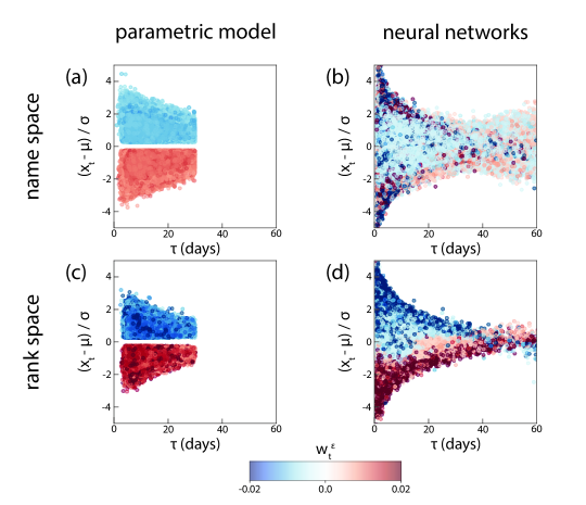
Figure 10: Portfolio weights in residual space: parametric model versus neural networks. We illustrate the behavior of both the parametric model and neural networks by analyzing the relationship between the input, the trajectories of cumulative residual returns $x_{t}^{L}$, and the output, the portfolio weights in residual space, $w_{t}^{\epsilon}$. To visualize the relationship, the cumulative residual return trajectories $x_{t}^{L}$ are first fitted to an OU process in Eq. 2.2.4 and parameterized by two variables: (i) deviation from long-term average $\frac{x_{t}-\mu}{\sigma}$, and (ii) mean-reverting time $\tau$. After the parametrization, each trajectory corresponds to a point in a two-dimensional space spanned by these two variables. We further color-code these points by the portfolio weights in residual space $w_{t}^{\epsilon}$. This analysis is performed with $w_{t}^{\epsilon}$ calculated by four scenarios: (a) the parametric model in name space; (b) neural networks in name space; (c) the parametric model in rank space; (d) neural networks in rank space. The interpretation of these results is detailed in section 3.5.

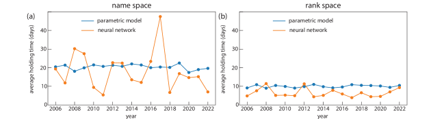
Figure 11: Average holding time. The holding time is defined as the maximum length of the time interval during which the portfolio weights in residual space $w_{i,t}$ remain non-zero. The holding time is presented as an average over each calendar year. We consider results from four scenarios: (a) parametric model in name space (blue line) and neural networks in name space (orange line); (b) parametric model in rank space (blue line) and neural network in rank space (orange line). For the portfolios from the parametric model, the average holding time yields $\sim 20$ days in name space and $\sim 10$ days in rank space. For the portfolios from neural networks, the average holding time for portfolios in rank space is further reduced, contrasting the volatile and high average holding time in name space. This stark contrast echoes different training efficiency between name space and rank space (Fig. 12).

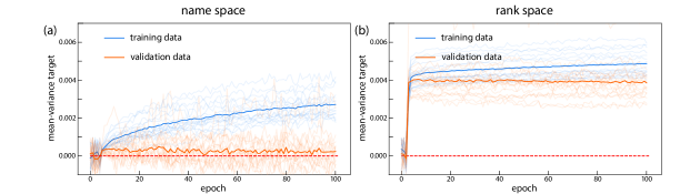
Figure 12: Traing curves of neural networks. (a, b) We show the mean-variance target as a function of training epochs for neural networks as specified by Eq. 2.2.13 in name space (a) and by Eq. 2.2.13 in rank space (b). The training curves originate from the phase I training process focusing on hyperparameter tuning. To evaluate the out-of-sample portfolio weights from trading day $t$ to $t+252$, we use the training data from day $t-1000$ to day $t-60$ and validation data from day $t-59$ to $t-1$ as the validation data. The neural networks are re-trained annually with random initialization, yielding approximately 17 training curves from 2006 to 2022. The transparent lines show individual training curves with their average represented by the opaque lines. The neural networks in rank space are more efficiently trained than those in name space.

3.6 Estimating a characteristic time between rank switching for intraday rebalancing

The rebalancing interval, $\mathcal{T}$, turns out to be a crucial parameter for statistical arbitrage portfolios in rank space. To demonstrate, we present the calculated PnL with varying rebalancing intervals in Fig. 13(a), where the portfolio weights are calculated from the neural networks in rank space. The associated average Sharpe ratio and terminal PnL as a function of the rebalancing interval are summarized in Fig. 13(b), with both peaking at 225 minutes.

Here, we delve into the rationale behind the optimal 225-minute interval, starting with an examination of two proximate capitalization processes modeled as Brownian motions, $c_{1,t}$ and $c_{2,t}$ (Fig. 13(c)). Given that transaction costs from intraday rebalancing primarily arise from rank swaps in capitalization (section 2.3), we measure the cumulative time $\Lambda(t)$ that the capitalization processes cross (Fig. 13(c), red line),

$$\Lambda(t)=\lim_{\delta\downarrow 0}\int_{0}^{t}\boldsymbol{1}_{\{|c_{1,\tau}-c_{2,\tau}|\leq\delta\}}d\tau$$ (3.6.1)

The rank-swapping interval $\lambda$ is defined as the time between the cross of capitalization processes, or equivalently, the increments of $\Lambda(t)$. This classical interacting Brownian system features two characteristic regimes: (i) the idle regime, where the two capitalization processes are distant, maintaining constant $\Lambda(t)$ with prolonged $\lambda$; (ii) the collision regime (highlighted in brown shaded area in Fig. 13(c)), where the two capitalization processes stay close, leading to rapid increases in $\Lambda(t)$ and short $\lambda$. We show the empirical distribution of $\lambda$ on real market in Fig. 13(d), where the small $\lambda$ values arise from the collision regime and larger $\lambda$ values from the idle regime, following approximately an exponential distribution as a typical signature for standard Brownian particle systems. The 225 minutes is situated at the intersection of the two regimes, establishing it as a characteristic time for rank switching.

In the detailed analysis of the intraday rebalancing in Eq. 2.3.6 and Fig. 4, the transaction costs arise from (i) latency costs due to delayed reactions post-rank-swapping, and (ii) costs from bid-ask spreads incurred during active trading. For the collision regime in Fig. 13(c), it is preferable to delay trading to minimize bid-ask spread costs. Conversely, in the idle regime, immediate trading is preferable to reduce latency costs. The 225-minute interval effectively differentiates these regimes, thus optimizing overall transaction costs.

The discussion above highlights the challenge in trading ranks – discerning between the collision and idle regimes and trading at their intersection. Our current intraday rebalancing approach crudely harnesses average behavior of U.S. equity market, and leaves considerable scope for enhancement that we will follow up on in subsequent research papers.

Figure 13: PnL dependence on rebalancing interval and characteristic rank-swapping time. (a) The PnL across various intraday rebalancing intervals $\mathcal{T}$ to realize the rank return in continuous time limit $\tilde{r}_{t}$. The underlying portfolio weights are derived from the neural networks in rank space. (b) Averaged Sharpe ratio between 2006 and 2022 and the terminal PnL as functions of rebalance intervals from (a). Both metrics peak at $\mathcal{T}=225$ minutes. (c) Schematic representation of two capitalization processes,$c_{1}$ and $c_{2}$. The $\Lambda(t)$ measures the cumulative time that the capitalization processes $c_{1}$ and $c_{2}$ cross. Rank switching time $\lambda$ is the interval between the increments in local time. This stochastic system has two characteristic regimes: (i) the idle regime, where the two capitalization processes are distant, maintaining constant $\Lambda(t)$ with prolonged $\lambda$; (ii) the collision regime (highlighted in brown shaded area in Fig. 13(c)), where the two capitalization processes stay close, leading to rapid increases in $\Lambda(t)$ and short $\lambda$. (e) The empirical distributions of rank-swapping time $\tau$ based on the intraday market data. Low (high) $\lambda$ arises from the ”idle” (”collision”) regime. The red dashed line marks the optimal rebalancing interval, $\mathcal{T}=225$ minutes, positioned at the intersection between the idle and collision regimes, suggesting it is a balanced choice for minimizing transaction costs while responding effectively with rank-swapping events.

3.7 Dependence on transaction cost and dollar neutrality

Here, we discuss the dependence of the portfolio performance on transaction costs and dollar neutrality. First, we present its sensitivity to transaction costs. We show the PnL with different transaction cost factor $\eta$ in Fig. 14(a) and the corresponding Sharpe ratio in Fig. 14. The current strategy shows significant sensitivity to the transaction cost factor and stops to profit with $\eta=5$ basis points. A more effective strategy to trade ranks will likely help the strategy more immune to transaction costs.

Second, we characterize the long or short proportion of the portfolio weights in equity space, $\sum_{i:w_{i,t}^{R}>0}w_{i,t}$ or $\sum_{i:w_{i,t}^{R}<0}w_{i,t}$ and the dollar neutrality, $\frac{\sum_{i}w_{i,t}^{R}}{\sum_{i}|w_{i,t}^{R}|}$. The results are presented in Fig. 15(a1-d1) and Fig. 15(a2-d2), where we consider $w_{t}^{R}$ calculated by four scenarios: (i) the parametric model in name space (Fig. 15(a1, a2), (ii) neural networks in name space (Fig. 15(b1, b2), (iii) the parametric model in rank space (Fig. 15(c1, c2), (iv) neural networks in rank spce (Fig. 15(d1, d2)). Notably, the long or short proportion of $w_{t}^{R}$ by neural networks (Fig. 15(b1, d1)) is much more volatile than those by the parametric model (Fig. 15(a1, c1)), as a result of flexible leverage adopted by neural networks. However, the dollar neutrality is satisfied on average thanks to the market neutrality of the portfolios.

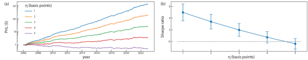
Figure 14: PnL dependence on transaction cost factor $\eta$. (a) The PnL with varing levels of the transaction cost factor $\eta$. The underlying portfolio weights are derived from the neural networks in rank space. (b) The average Sharpe ratio from 2006 to 2022 at different values of $\eta$ derived from (a). The strategy stops to profit with 5 basis points transaction costs due to substantial costs associated with realizing rank returns in continuous time limit. The significant change in Sharpe ratio under varying transaction costs underscores the strategy’s sensitivity to transaction costs and motivates ongoing improvements in ”trading ranks”.

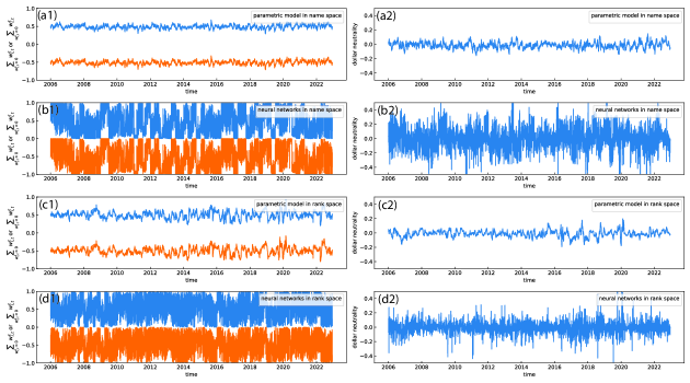
Figure 15: Portfolio weights in residual return and dollar neutrality. (a1-d1) The temporal dependence of average long/short portfolio weights in residual space, $\sum_{w_{i,t}^{\epsilon}>0}w_{i,t}^{\epsilon}$ and $\sum_{w_{i,t}^{\epsilon}<0}w_{i,t}^{\epsilon}$. (a2-d2) The deviation from dollar neutrality measured by $\frac{\sum_{i}w_{i,t}^{R}}{\sum_{i}|w_{i,t}^{R}|}$. We consider four scenarios: (a1-a2) parametric model in name space; (b1-b2) neural networks in name space; (c1-c2) parametric model in rank space; (d1-d2) neural networks in rank space.

4 Summary and conclusion

In conclusion, we have introduced a novel statistical arbitrage strategy that anchors on the market dynamics in rank space. Our statistical arbitrage framework features an intraday rebalancing mechanism for effective conversion between name space and rank space and adopts both the parametric model and neural networks to calculate portfolio weights. The derived statistical arbitrage portfolios in rank space consistently outperform their counterparts in name space without transaction costs. Such improved performance is inherited from robust market representation and enhanced mean-reverting properties of residual returns in rank space. However, due to the substantial transaction costs associated with realizing rank returns in the continuous-time limit, the portfolios derived from the parametric model in rank space cease to profit with transaction costs. Fortunately, by leveraging the neural networks, the portfolios derived from the neural networks in rank space yield an average annual return of 35.68% and an average Sharpe ratio of 3.28 from 2007 to 2022 with 2 basis points transaction costs. Motivated by the performance, a closer inspection of the neural networks suggests the following refined trading philosophy compared to the parametric model: (i) applying adjustable leverage based on the magnitude of long-term deviations, and (ii) minimizing the carry time before liquidation to reduce the exposure to carry-on risk.

Our pioneering investigation into statistical arbitrage in rank space also unveils multiple avenues for further research in at least two aspects. Theoretically, our empirical observations on the contrasts of residual space between name space and rank space will motivate more explanatory models. For practitioners, the comparisons in portfolio performances with and without transaction costs (Fig. 9, Table 1, Table 2) highlight the main challenge for statistical arbitrage in rank space – realizing rank returns in continuous-time limits. While we propose the intraday rebalancing that crudely utilizes the characteristic rank-switching time in U.S. equity market, there likely remains abundant room to optimize the strategy and improve the portfolio performance, which will be followed up in our subsequent research efforts.

5 Appendix

5.1 $\Phi_{t}\beta_{t}=0$

Here, we prove the equality $\Phi_{t}\beta_{t}=0$, crucial relationship for market neutrality. We denote the return matrix $R_{t}=(r_{t-T+1},r_{t-T+2},...,r_{t})\in\mathbb{R}^{N\times T}$. Assume singular value decomposition of $R_{t}$,

$$R_{t}-R_{f}=U\Sigma V^{T}$$ (5.1.1)

, where $R_{f}\in\mathbb{R}^{1\times T}$ is the risk-free rate, $U\in\mathbb{R}^{N\times N}$, $\Sigma\in\mathbb{R}^{N\times T}$, and $V^{T}\in\mathbb{R}^{T\times T}$. Then, the factors and loadings in Eq. 2.1.1 and $\omega_{t}$ in Eq. 2.1.2 becomes

$$F_{t}=\begin{pmatrix}v_{1}^{T}\\ v_{2}^{T}\\ ...\\ v_{K}^{T}\end{pmatrix},\quad\beta_{t}=\begin{pmatrix}u_{1},u_{2},...,u_{K}\end{pmatrix}\begin{pmatrix}\sigma_{1}&&\\ &...&\\ &&\sigma_{K}\end{pmatrix},\quad\omega_{t}=\begin{pmatrix}\sigma_{1}^{-1}&&\\ &...&\\ &&\sigma_{K}^{-1}\end{pmatrix}\begin{pmatrix}u_{1}^{T}\\ u_{2}^{T}\\ ...\\ u_{K}^{T}\end{pmatrix}$$ (5.1.2)

, where $u_{i}$ and $v_{i}$ are the $i$-th column of matrix $U$ and $V$. Then, because $U$ and $V$ are orthogonal matrix,

$$\beta_{t}\omega_{t}=I$$ (5.1.3)

$$\implies \Phi_{t}\beta_{t}=(I-\beta_{t}\omega_{t})\beta_{t}=0$$

.

5.2 Parameter estimation for OU process

The OU process can be viewed as a 1-lag autoregressive process in continuous-time limit. Therefore, we carry out linear regression to fit the cumulative residual return $x_{t}^{L}$ (Eq. 2.2.1) to the OU process (Eq. 2.2.4),

$$x_{t-L+\alpha}=a+bx_{t-L+\alpha-1}+\xi_{t-L+\alpha},\quad\alpha=1,2,...,L$$ (5.2.1)

The coefficients between the OU process and the 1-lag autoregressive process are related by[3]

$$\begin{cases}&a=m(1-e^{-\kappa\Delta t}\\ &b=e^{-\kappa\Delta t}\\ &\text{Variance}(\xi)=\sigma^{2}\frac{1-e^{-2\kappa\Delta t}}{2\kappa}\end{cases}\Leftrightarrow\begin{cases}\kappa&=-\log(b)\times 252\\ m&=\frac{a}{1-b}\\ \sigma&=\sqrt{\frac{\text{Variance}(\xi_{t})}{1-b^{2}}}\end{cases}$$ (5.2.2)

References

• [1] F. Acero, P. Zehtabi, N. Marchesotti, M. Cashmore, D. Magazzeni, and M. Veloso, Deep reinforcement learning and mean-variance strategies for responsible portfolio optimization, arXiv:2403.16667, (2024).
• [2] M. Avellaneda, B. Healy, A. Papanicolaou, and G. Papanicolaou, Principal eigenportfolios for US equities, SIAM Journal on Financial Mathematics, 13 (2022), pp. 702–744.
• [3] M. Avellaneda and J.-H. Lee, Statistical arbitrage in the US equities market, Quantitative Finance, 10 (2010), pp. 761–782.
• [4] J. L. Ba, J. R. Kiros, and G. E. Hinton, Layer normalization, arXiv:1607.06450, (2016).
• [5] A. D. Banner, R. Fernholz, and I. Karatzas, Atlas models of equity markets, Annals of applied probability, 15 (2005), pp. 2296–2330.
• [6] Á. Cartea, S. Jaimungal, and J. Penalva, Algorithmic and high-frequency trading, Cambridge University Press, 2015.
• [7] J. Devlin, M.-W. Chang, K. Lee, and K. Toutanova, Bert: Pre-training of deep bidirectional transformers for language understanding, arXiv:1810.04805, (2018).
• [8] P. K. Diederik, Adam: A method for stochastic optimization, (2014).
• [9] E. F. Fama and K. R. French, The cross-section of expected stock returns, the Journal of Finance, 47 (1992), pp. 427–465.
• [10]  , A five-factor asset pricing model, Journal of financial economics, 116 (2015), pp. 1–22.
• [11] E. R. Fernholz and E. R. Fernholz, Stochastic portfolio theory, Springer, 2002.
• [12] J. Guijarro-Ordonez, M. Pelger, and G. Zanotti, Deep learning statistical arbitrage, arXiv:2106.04028, (2021).
• [13] K. He, X. Zhang, S. Ren, and J. Sun, Deep residual learning for image recognition, Proceedings of the IEEE conference on computer vision and pattern recognition, (2016), pp. 770–778.
• [14] B. Healy, Y.-F. Li, A. Papanicolaou, and P. Papanicolaou, Robust representation of the U.S. equity market: name space versus rank space, working paper, (2024).
• [15] T. Ichiba, V. Papathanakos, A. Banner, I. Karatzas, and R. Fernholz, Hybrid atlas models, Annals of applied probability, 21 (2011), pp. 609–644.
• [16] I. Karatzas and R. Fernholz, Stochastic portfolio theory: an overview, Handbook of numerical analysis, 15 (2009), pp. 89–167.
• [17] T. Kim and H. Y. Kim, Optimizing the pairs-trading strategy using deep reinforcement learning with trading and stop-loss boundaries, Complexity, 2019 (2019), p. 3582516.
• [18] T. S.-t. Leung and X. Li, Optimal mean reversion trading: Mathematical analysis and practical applications, vol. 1, World Scientific, 2015.
• [19] A. Onatski, Determining the number of factors from empirical distribution of eigenvalues, The Review of Economics and Statistics, 92 (2010), pp. 1004–1016.
• [20] C. Szegedy, W. Liu, Y. Jia, P. Sermanet, S. Reed, D. Anguelov, D. Erhan, V. Vanhoucke, and A. Rabinovich, Going deeper with convolutions, Proceedings of the IEEE conference on computer vision and pattern recognition, (2015), pp. 1–9.
• [21] A. Tourin and R. Yan, Dynamic pairs trading using the stochastic control approach, Journal of Economic Dynamics and Control, 37 (2013), pp. 1972–1981.
• [22] D. Ulyanov, A. Vedaldi, and V. Lempitsky, Instance normalization: The missing ingredient for fast stylization, arXiv:1607.08022, (2016).
• [23] A. Vaswani, N. Shazeer, N. Parmar, J. Uszkoreit, L. Jones, A. N. Gomez, Ł. Kaiser, and I. Polosukhin, Attention is all you need, Advances in neural information processing systems, 30 (2017).
• [24] J. Yeo and G. Papanicolaou, Risk control of mean-reversion time in statistical arbitrage, Risk and Decision Analysis, 6 (2017), pp. 263–290.