Open loop calibration and closed loop non perturbative estimation of the lateral errors of an adaptive optics system: examples with GRAVITY+ and CHARA experimental data

Abstract

Performances of an adaptive optics (AO) system are directly linked with the quality of its alignment. During the instrument calibration, having open loop fast tools with a large capture range are necessary to quickly assess the system misalignment and to drive it towards a state allowing to close the AO loop. During operation, complex systems are prone to misalignments (mechanical flexions, rotation of optical elements, …) that potentially degrade the AO performances, creating a need for a monitoring tool to tackle their driftage. In this work, we first present an improved perturbative method to quickly assess large lateral errors in open loop. It uses the spatial correlation of the measured interaction matrix of a limited number of 2D spatial modes with a synthetic model. Then, we introduce a novel solution to finely measure and correct these lateral errors via the closed loop telemetry. Non-perturbative, this method consequently does not impact the science output of the instrument. It is based on the temporal correlation of 2D spatial frequencies in the deformable mirror commands. It is model-free (no need of an interaction matrix model) and sparse in the Fourier space, making it fast and easily scalable to complex systems such as future extremely large telescopes. Finally, we present some results obtained on the development bench of the GRAVITY+ extreme AO system (Cartesian grid, 1432 actuators). In addition, we show with on-sky results gathered with CHARA and GRAVITY/CIAO that the method is adaptable to non-conventional AO geometries (hexagonal grids, 60 actuators).

1 INTRODUCTION

The role of an Adaptive Optics (AO) system is to compensate for the wavefront corrugations induced by atmospheric turbulence[Roddier:99_AO_system]. To do so, such a system is composed by a wavefront sensor (WFS) whose measurements are analyzed by a real time computer (RTC) and converted into a set of commands sent to a deformable mirror (DM) that corrects the optical aberrations. To be effective, this feedback loop must run faster than the turbulence temporal evolution, with typical frequencies ranging from several hundred Hertz to a kilo-Hertz.

Any alignment error in the AO system degrades its performances, or even worse, destabilizes the AO loop. Fine registration of the couple DM/WFS is thus critical. Among others, see Heritier:19_PHD (Sec. 2.1), the classical (and most impacting) mis-registrations are the $x$ and $y$-shifts (lateral translation of the DM with respect to the WFS), the clocking (rotation of the DM with respect to the WFS), and the magnification and anamorphosis (stretches of the DM with respect to the WFS).

If different techniques exist to assess the mis-registration state of an AO systemKolb:16_SPIE_Review_AO_calibration, most of the tools to track mis-registrations use the interaction matrix (IM) of the AO systemRoddier:99_AO_system that links the commands sent to the DM to the measures provided by the WFS. These techniques rely on the fact that an alignment error in the AO system leaves a measurable signal in its IM.

In early AO systems, IMs were experimentally calibrated on instrument internal sources with high signal-to-noise ratios (S/Ns)Oberti:06_SPIE_PSIM_vs_measured_IM. But the arrival of telescopes with adaptive secondary mirrors, such as the Multiple Mirror TelescopeBrusa:03_MMT, the Large Binocular TelescopeRiccardi:03_SPIE_LBT_SDM, or the AOFStrobele:06_SPIE_AOF, changed the deal. Without any reference source, the IM must be measured directly on-sky at night. This raised new challengesOberti:06_SPIE_PSIM_vs_measured_IM; Pinna:12_SPIE_FLAO; Lai:21_DO_CRIME; Kolb:16_SPIE_Review_AO_calibration: freezing the turbulence, fighting low S/N, minimizing the loss of precious night time for the scientific observations, …

Thus, new methods emerged, based on the physical modeling of the interaction matrix, so-called synthetic IMOberti:06_SPIE_PSIM_vs_measured_IM; Kolb:12_SPIE_AOF; Heritier:18_PyWFS_calibration; Heritier:19_PHD. The mis-registration parameters are fitted through dedicated calibrations, on internal sources or on-skyOberti:04_SPIE_IM_misreg; Neichel:12_SPIE_MCAO; Kolb:16_SPIE_Review_AO_calibration; Heritier:18_PyWFS_calibration to obtain noiseless pseudo-synthetic interaction matricesOberti:06_SPIE_PSIM_vs_measured_IM (PSIMs).

Nonetheless, mis-registrations are susceptible to evolve during observation (mechanical flexion, thermal evolution, …). And future Extremely Large TelescopesJohns:06_SPIE_GMT; Gilmozzi:07_ELT; Boyer:18_SPIE_TMT(ELTs) will bring this challenge to other levels: always more complex (and time consuming) PSIM models, increasing number of actuators, non-linear WFSs, unprecedented distances between DMs and WFSs (with moving/rotating parts in-between prone to misalignment), … It then becomes impossible to perform regular calibrations and it is thus necessary to track the evolution of the mis-registrations directly during the scientific acquisitions with online tools for AO system auto-calibration.

In this context we developed two news methods to assess lateral mis-registration in an AO system that relax the need of complex PSIM model fitting. The first one, see Sec. 2, is based on a perturbative approach whereby two-dimensional (2D) modes are applied on the system. It has a large capture range and can be used in open loop in order to calibrate and preset the AO system. The second one, see Sec. 3, is a non-perturbative approach analyzing correlation signals in the AO loop telemetry. Working in closed loop, it can be used in real time to monitor the system mis-registration without impacting the science acquisition.

These methods have been introduced in a previous paper, see Berdeu:24_misreg and implemented in the Standard Platform for Adaptive optics Real Time ApplicationsSuarez:12_SPIE_SPARTA; Shchekaturov:23_SPARTA_upgrade; Dembet:23_RTC_GPAO (SPARTA), the RTC of GRAVITY+GRAVITYplus:22_messenger. In this work, we present new data, obtained on the GRAVITY+ AO development benchMillour:22_SPIE_GPAO_bench; LeBouquin:23_GPAO_design(GPAO), as well as the first on-sky results obtained from the Center for High Angular Resolution AstronomyAnugu:2020_CHARA_SPIE (CHARA) and the Coudé Infrared Adaptive OpticsKendrew:12_CIAO (CIAO) of GRAVITYGRAVITY:17_VLTI. For each technique, (i) a brief reminder of the method is introduced, see Secs. 2.1 and 3.1; (ii) then experimental results are given, see Secs. 2.2 and 3.2.

2 Perturbative 2D modal estimator

2.1 Overview of the Method

2.1.1 General concept

The idea of the method is summed up in Fig. 1. When a spatial pattern is applied on the DM, see Fig. 1a, a specific spatial pattern is seen in the SH-WFS data, see Fig. 1b. In the following, we used a modal approach based on Karhunen–Loève (KL) functionsDai:95_KL applied on the DM commands (modal IM). If the considered modes are properly sampled, a lateral mis-registration geometrically shifts the measurements, see Fig. 1c. Thus, the 2D spatial correlation of a measured modal IM with a reference modal IM should be usable as a lateral error estimator.

DM $35^{\text{th}}$ KL mode	Reference slopes	Measured slopes	Modal correlation	Inverse problem
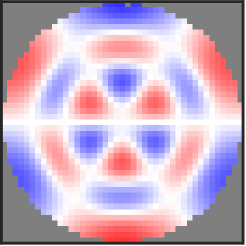
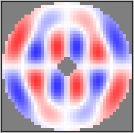
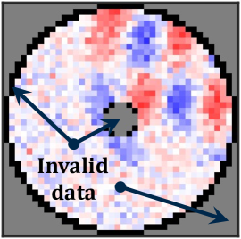
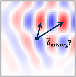
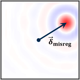
(a)	(b)	(c)	(d)	(e)

Figure 1: Simulated example of the spatial 2D correlation method. Panel a: KL mode applied on the DM. Panel b: Corresponding reference slopes on the WFS. Panel c: Slopes of the measured partial IM. Panel d: Standard correlation of the measured KL mode with the reference. Panel e: Global inverse problem approach on all the measured modes.

Noting ${\boldsymbol{M}}^{\text{int}}_{m}\left({{\boldsymbol{{x}}}}\right)$ (resp. $\tilde{{\boldsymbol{M}}}^{\text{int}}_{m}\left({{\boldsymbol{{x}}}}\right)$) the reference modal IM of the system without any mis-registration (resp. the measured modal IM) of the KL mode $m$, the cross-correlation of the 2D IMs for a shift ${{\boldsymbol{\delta}}}$ is given by:

$$\left[\tilde{{\boldsymbol{M}}}^{\text{int}}_{m}\mathbin{\mathchoice{\ooalign{$\displaystyle\vbox{\hbox{\scalebox{0.77778}{$\displaystyle\bigcirc$}}}$\cr$\displaystyle\star$\cr}}{\ooalign{$\textstyle\vbox{\hbox{\scalebox{0.77778}{$\textstyle\bigcirc$}}}$\cr$\textstyle\star$\cr}}{\ooalign{$\scriptstyle\vbox{\hbox{\scalebox{0.77778}{$\scriptstyle\bigcirc$}}}$\cr$\scriptstyle\star$\cr}}{\ooalign{$\scriptscriptstyle\vbox{\hbox{\scalebox{0.77778}{$\scriptscriptstyle\bigcirc$}}}$\cr$\scriptscriptstyle\star$\cr}}}{\boldsymbol{M}}^{\text{int}}_{m}\right]\left({{\boldsymbol{\delta}}}\right){}\triangleq{}\sum_{{{\boldsymbol{{x}}}}}\tilde{{\boldsymbol{M}}}^{\text{int}}_{m}\left({{\boldsymbol{{x}}}}\right){\boldsymbol{M}}^{\text{int}}_{m}\left({{\boldsymbol{{x}}}}-{{\boldsymbol{\delta}}}\right){}={}\alpha\left({{\boldsymbol{\delta}}}\right)\,.$$ (1)

In presence of a lateral mis-registration, Eq. (1) would give maps similar to Fig. 1d. Performed on a single mode, such correlation maps can lead to ambiguities in the determination of the maximum location and to poor sensitivity. In our method, we rather define the merit criterion in terms of how similar the two IMs are in terms of mean squares, jointly accounting for all the modes,

$$\alpha\left({{\boldsymbol{\delta}}}\right)=\underset{\beta}{\text{argmin}}\;\sum_{{{\boldsymbol{{x}}}},m}w\left({{\boldsymbol{{x}}}},{{\boldsymbol{\delta}}}\right)\left(\tilde{{\boldsymbol{M}}}^{\text{int}}_{m}\left({{\boldsymbol{{x}}}}\right)-\beta{\boldsymbol{M}}^{\text{int}}_{m}\left({{\boldsymbol{{x}}}}-{{\boldsymbol{\delta}}}\right)\right)^{2}\,,\text{ with }w\left({{\boldsymbol{{x}}}},{{\boldsymbol{\delta}}}\right)={w}^{\text{valid}}\left({{\boldsymbol{{x}}}}\right){w}^{\text{wfs}}\left({{\boldsymbol{{x}}}}-{{\boldsymbol{\delta}}}\right)\,,$$ (2)

where ${w}^{\text{wfs}}\left({{\boldsymbol{{x}}}}\right)$ is the map of the valid subapertures in the PSIM model and ${w}^{\text{valid}}\left({{\boldsymbol{{x}}}}\right)$ is the map of the valid subapertures in the measurements, discarding poorly illuminated subapertures. Equation (2) has an analytical solution given by:

$$\alpha\left({{\boldsymbol{\delta}}}\right){}={}\frac{\sum_{{{\boldsymbol{{x}}}},m}w\left({{\boldsymbol{{x}}}},{{\boldsymbol{\delta}}}\right)\tilde{{\boldsymbol{M}}}^{\text{int}}_{m}\left({{\boldsymbol{{x}}}}\right){\boldsymbol{M}}^{\text{int}}_{m}\left({{\boldsymbol{{x}}}}-{{\boldsymbol{\delta}}}\right)}{\sum_{{{\boldsymbol{{x}}}},m}w\left({{\boldsymbol{{x}}}},{{\boldsymbol{\delta}}}\right)\left[{\boldsymbol{M}}^{\text{int}}_{m}\left({{\boldsymbol{{x}}}}-{{\boldsymbol{\delta}}}\right)\right]^{2}}{}={}\frac{\sum_{m}\left[{w}^{\text{valid}}\tilde{{\boldsymbol{M}}}^{\text{int}}_{m}\mathbin{\mathchoice{\ooalign{$\displaystyle\vbox{\hbox{\scalebox{0.77778}{$\displaystyle\bigcirc$}}}$\cr$\displaystyle\star$\cr}}{\ooalign{$\textstyle\vbox{\hbox{\scalebox{0.77778}{$\textstyle\bigcirc$}}}$\cr$\textstyle\star$\cr}}{\ooalign{$\scriptstyle\vbox{\hbox{\scalebox{0.77778}{$\scriptstyle\bigcirc$}}}$\cr$\scriptstyle\star$\cr}}{\ooalign{$\scriptscriptstyle\vbox{\hbox{\scalebox{0.77778}{$\scriptscriptstyle\bigcirc$}}}$\cr$\scriptscriptstyle\star$\cr}}}{w}^{\text{wfs}}{\boldsymbol{M}}^{\text{int}}_{m}\right]\left({{\boldsymbol{\delta}}}\right)}{\sum_{m}\left[{w}^{\text{valid}}\mathbin{\mathchoice{\ooalign{$\displaystyle\vbox{\hbox{\scalebox{0.77778}{$\displaystyle\bigcirc$}}}$\cr$\displaystyle\star$\cr}}{\ooalign{$\textstyle\vbox{\hbox{\scalebox{0.77778}{$\textstyle\bigcirc$}}}$\cr$\textstyle\star$\cr}}{\ooalign{$\scriptstyle\vbox{\hbox{\scalebox{0.77778}{$\scriptstyle\bigcirc$}}}$\cr$\scriptstyle\star$\cr}}{\ooalign{$\scriptscriptstyle\vbox{\hbox{\scalebox{0.77778}{$\scriptscriptstyle\bigcirc$}}}$\cr$\scriptscriptstyle\star$\cr}}}{w}^{\text{wfs}}\left[{\boldsymbol{M}}^{\text{int}}_{m}\right]^{2}\right]\left({{\boldsymbol{\delta}}}\right)}\,.$$ (3)

Equation (3) is the ratio of the modal sum of 2D cross-correlations and the position of the global maximum of the obtained map, see Fig. 1e, gives the estimated lateral mis-registration $\tilde{{{\boldsymbol{\delta}}}}$ in a single pass:

$$\tilde{{{\boldsymbol{\delta}}}}=\underset{{{\boldsymbol{\delta}}}}{\text{argmax}}\;\alpha\left({{\boldsymbol{\delta}}}\right)\,.$$ (4)

As discussed in Berdeu:24_misreg, this map can be up-sampled to perform super-resolution.

2.2 Experimental Results

Figure 2 gathers some screenshots of the SPARTA panels that show the use of the proposed method during the present of the visible mode of GPAO, based on a $40\!\times\!40$ Shack-Hartmann WFS (SH-WFS) and a DM with 1432 active actuators. The turbulence was emulated with a plate, producing a wind of $v_{0}\simeq$8.4\text{\,}\mathrm{m}\text{\,}{\mathrm{s}}^{-1}$$ with a Fried parameter of $r_{0}\simeq$14\text{\,}\mathrm{cm}$$.

(a)

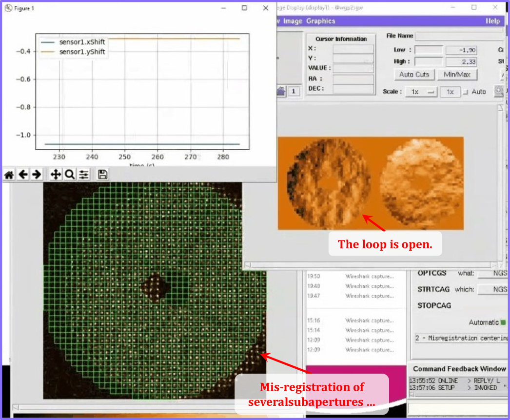
(b)

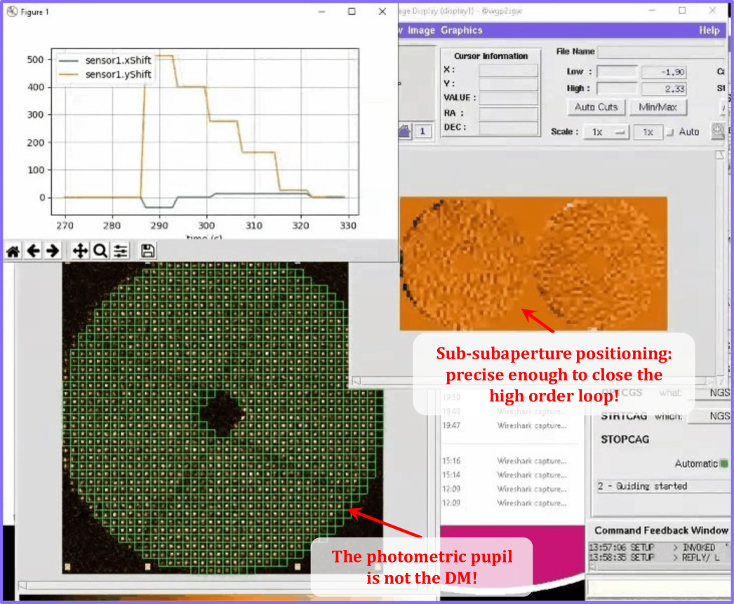
Figure 2: Screenshots of the spatial 2D correlation method in the GPAO bench. The orange and blue curves are the $x$ and $y$ outputs of the estimator according to time. The SH-WFS spots are displayed in the bottom left and the corresponding $x$ and $y$ slopes are given side by side in the windows with the orange look up table. Panel a: Initial state of the AO system with a lateral error of several subapertures. Panel b: System after convergence of the lateral error corrective loop.

In the initial state, see Fig. 2a, the loop is open and the system is misaligned by several subapertures. This is visible by the important shift between the photometric pupil (SH-WFS spots) relative to the SH-WFS geometry (green boxes). Figure 2b shows the system after the convergence of the corrective loop that monitors the lateral error based on the 2D modal estimator. The system has converged in a few iterations and the alignment is good enough to close the high order AO loop, with 800 controlled modes.

As emphasized by the red arrow, an alignment of the DM with respect to the WFS does not correspond to the alignment of the photometric pupil. This is explained by the fact that in GPAO, the DM clear aperture is larger than the telescope pupil image and thus photometry centering cannot be used to register the couple DM/WFS.

The algorithm has been tested in the bench with the different GPAO modes ($9\!\times\!9$, $30\!\times\!30$, $40\!\times\!40$ SH-WFSs) and with different phase plates and source powers, spanning a large variety of conditions. In all cases, it successfully brings the system to a state where the high order AO loop closes stably. The mis-registration monitoring can thus then switch to the closed loop estimator, as discussed below.

3 Non-perturbative closed loop estimator

3.1 Overview of the Method

As summed by the blue (or green) block diagram of Fig. 3a, an AO loop works as follows:

• the WFS $S$ converts the 2D wavefront ${\boldsymbol{w}}$ into measurements ${\boldsymbol{m}}$ corrupted by noise, ${\boldsymbol{n}}$: ${\boldsymbol{m}}=S\left({\boldsymbol{w}}\right)+{\boldsymbol{n}}$,

• these measurements are converted via ${\boldsymbol{M}}^{\text{cmd}}$, the command matrix (computed by inverting the PSIM of the system filtered on a given $n^{\text{mod}}$ number of KL modes), to a command correction ${\boldsymbol{c}}^{\delta}={\boldsymbol{M}}^{\text{cmd}}{\boldsymbol{m}}$,

• the controller $C$, for example a leaky integrator of leak gain $g^{\epsilon}$ and integral gain $g^{\int}$, computes a new command ${\boldsymbol{c}}^{i+1}=\left(1-g^{\epsilon}\right){\boldsymbol{c}}^{i}+g^{\int}{\boldsymbol{c}}^{\delta}$,

• this command is applied on the DM actuators $C$ until the next command arrives.

All the above steps are linear. Thus, the AO loop can be described in the Fourier space of the commands ${\boldsymbol{m}}$, that is to say in terms of spatial frequencies ${{\boldsymbol{k}}}=\left(k_{x},k_{y}\right)$ ($\text{\,}{\mathrm{m}}^{-1}$) propagating through the system. The transfer functionsAstrom:21_Feedback_system in the temporal frequency space $f$ ($\text{\,}\mathrm{Hz}$) of each block of Fig. 3a are given byMadec:99_control

• $S\left(f\right)=\frac{1-e^{-2i\pi\tau^{\text{wfs}}f}}{2i\pi\tau^{\text{wfs}}f}$, where $\tau^{\text{wfs}}$ is the WFS exposure time,

• $C\left(f\right)=\frac{g^{\int}e^{-2i\pi\tau^{\text{lat}}f}}{1-\left(1-g^{\epsilon}\right)e^{-2i\pi\tau^{\text{rtc}}f}}$, where $\tau^{\text{lat}}$ is the latency of the system (communication and computation times) and $\tau^{\text{rtc}}$ is the period of the RTC cycle,

• $A\left(f\right)=\frac{1-e^{-2i\pi\tau^{\text{dm}}f}}{2i\pi\tau^{\text{dm}}f}$, where $\tau^{\text{dm}}$ is the holding time of the DM.

In general, all the characteristic times are equal: $\tau^{\text{lat}}\simeq\tau^{\text{dm}}\simeq\tau^{\text{wfs}}\simeq\tau^{\text{rtc}}$.

(a)

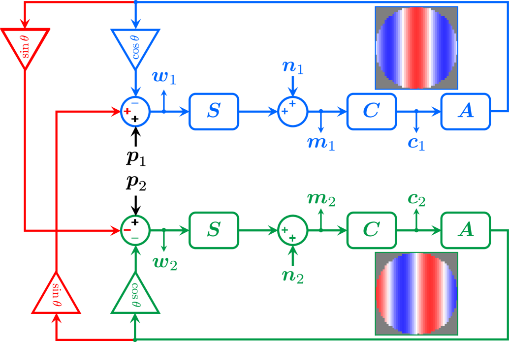
(b)

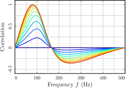
Figure 3: Temporal coupling of the spatial frequency ${{\boldsymbol{k}}}=\left(2/3D,0\right)$ in the AO loop telemetry. Panel a: Block diagram of the temporal coupling (in red) of the symmetric (cosine, in blue) and anti-symmetric (sine, in green) parts. Panel b: Imaginary part of the correlation curve ${\boldsymbol{\mathscr{C}}}_{\!{\boldsymbol{c}}_{1},{\boldsymbol{c}}_{2}}\left(\theta,f\right)$ in a noise limited regime with standard AO parameters $\tau^{\text{wfs}}=$1\text{\,}\mathrm{ms}$$, $g^{\int}=0.5$, $g^{\epsilon}=0$ and for various values of coupling coefficient $\theta$ from $0\text{\,}\mathrm{\SIUnitSymbolDegree}$ (blue) to $45\text{\,}\mathrm{\SIUnitSymbolDegree}$ (red), every $5\text{\,}\mathrm{\SIUnitSymbolDegree}$.

In the presence of a lateral mis-registration ${{\boldsymbol{\delta}}}=\left(\delta_{x},\delta_{y}\right)$, the spatially symmetric part of the commands ${\boldsymbol{c}}_{1}$ is partially projected on the spatially anti-symmetric part of the WFS measurements and propagates to the anti-symmetric part of the command ${\boldsymbol{c}}_{2}$ (and oppositely). This cross-coupling is emphasized by the red connectors in Fig. 3a, with a coupling coefficient of:

$$\theta=2\pi{{\boldsymbol{k}}}^{T}\!\!\cdot{{\boldsymbol{\delta}}}\,.$$ (5)

Thus, the commands ${\boldsymbol{c}}_{1}$ and ${\boldsymbol{c}}_{2}$ are thus no longer independent. In the (spatial and temporal) Fourier space, the correlation a given spatial frequency ${{\boldsymbol{k}}}$ at a temporal frequency $f$ is defined by:

$${\boldsymbol{\mathscr{C}}}_{\!{\boldsymbol{c}}_{1},{\boldsymbol{c}}_{2}}\left({{\boldsymbol{k}}},f\right)\triangleq\frac{\left\langle c_{1}\left({{\boldsymbol{k}}},f\right)\overline{c}_{2}\left({{\boldsymbol{k}}},f\right)\right\rangle}{\sqrt{{\boldsymbol{\mathscr{V}}}_{\!\!\!c_{1}}\left({{\boldsymbol{k}}},f\right){\boldsymbol{\mathscr{V}}}_{\!\!\!c_{2}}\left({{\boldsymbol{k}}},f\right)}}\text{ with }{\boldsymbol{\mathscr{V}}}_{\!\!\!{\boldsymbol{c}}_{i}}\left({{\boldsymbol{k}}},f\right)\triangleq\left\langle c_{i}\left({{\boldsymbol{k}}},f\right)\overline{c}_{i}\left({{\boldsymbol{k}}},f\right)\right\rangle\,.$$ (6)

Under the assumption that the different noise terms ${\boldsymbol{n}}_{i}$ and ${\boldsymbol{p}}_{i}$ are independent, we showed in Berdeu:24_misreg that:

$${\boldsymbol{\mathscr{C}}}_{\!{\boldsymbol{c}}_{1},{\boldsymbol{c}}_{2}}\left(\theta\left({{\boldsymbol{k}}}\right),f\right)/\theta\left({{\boldsymbol{k}}}\right)\underset{\theta\rightarrow 0}{\sim}2i\mathscr{I}\left[\frac{\overline{\mu}\left(f\right)}{1+\overline{\mu}\left(f\right)}\right]\triangleq i{\boldsymbol{\mathscr{C}}}_{\!0}\left(f\right)\text{ with }\mu\triangleq ACS\,.$$ (7)

The correlation of a given spatial frequency ${{\boldsymbol{k}}}$ is thus a pure imaginary number. Figure 3b shows the imaginary parts of the correlation ${\boldsymbol{\mathscr{C}}}_{\!{\boldsymbol{c}}_{1},{\boldsymbol{c}}_{2}}\left(\theta,f\right)$ for different values of the coupling coefficient $\theta$.

On the opposite side, in a pure frozen flow hypothesis (no noise propagation), of velocity ${{\boldsymbol{v}}}$, it comes with $f^{\parallel}={{\boldsymbol{k}}}^{T}\!\!\cdot{{\boldsymbol{v}}}$:

$$\forall\left\rvert f\right\lvert\neq f^{\parallel},\left\langle p_{1}\overline{p}_{2}\right\rangle\left(f\right)=0\text{ / }f=f^{\parallel},\mathscr{C}_{\!c_{1},c_{2}}\left(f^{\parallel}\right)\underset{\theta\rightarrow 0}{\sim}i\text{ / }f=-f^{\parallel},\mathscr{C}_{\!c_{1},c_{2}}\left(-f^{\parallel}\right)\underset{\theta\rightarrow 0}{\sim}-i\,.$$ (8)

This means that a frozen flow turbulence has a minimal impact on the correlation and only frequencies close to $f\simeq{{\boldsymbol{k}}}^{T}\!\!\cdot{{\boldsymbol{v}}}$ should be impacted.

In practice, as detailed in Berdeu:24_misreg, the symmetric (${\boldsymbol{c}}_{1}$) and anti-symmetric (${\boldsymbol{c}}_{2}$) parts of the commands ${\boldsymbol{c}}$ are extracted from the closed loop telemetry. Then, the imaginary part of the empirical correlation of the closed loop telemetry is estimated by:

$$\tilde{\mathscr{C}}^{\text{cl}}\left({{\boldsymbol{k}}},f\right)=\mathscr{I}\left[\frac{c_{1}\left({{\boldsymbol{k}}},f\right)\overline{c}_{2}\left({{\boldsymbol{k}}},f\right)}{\left\rvert c_{1}\left({{\boldsymbol{k}}},f\right)\right\lvert\left\rvert c_{2}\left({{\boldsymbol{k}}},f\right)\right\lvert}\right]\,.$$ (9)

And finally, the lateral error is then obtained from Eqs. (5) and (7) by solving:

$$\tilde{{{\boldsymbol{\delta}}}}=\underset{{{\boldsymbol{\delta}}}}{\text{argmin}}\;\sum_{{{\boldsymbol{k}}}\in\mathcal{K}^{\text{ctrl}},f>0}\left(\tilde{\mathscr{C}}^{\text{cl}}\left({{\boldsymbol{k}}},f\right)-2\pi{\boldsymbol{\mathscr{C}}}_{\!0}\left(f\right){{\boldsymbol{k}}}^{T}\!\!\cdot{{\boldsymbol{\delta}}}\right)^{2}\,,$$ (10)

where ${{\boldsymbol{k}}}\in\mathcal{K}^{\text{ctrl}}$ is the control space of the AO loop.

3.2 Experimental Results

3.2.1 On the GPAO bench

The estimator was tested in the GPAO bench inserting two phase screens in the bench to emulate a multi-layered atmosphere with an estimated global seeing of $\sim 1.1^{\prime\prime}$. In the initial state, a lateral mis-registration of 60 % of a subaperture $\Delta$ was injected in the system by translating the SH-WFS stage.

Figure 4a shows the convergence curve of the corrective loop in charge to re-align the system while in closed loop. The top panel shows the output of the closed loop estimator while the bottom panel shows the actual position of the WFS translation stage.

Lateral error update	2D spatial frequency space	Temporal frequency space
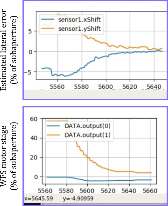
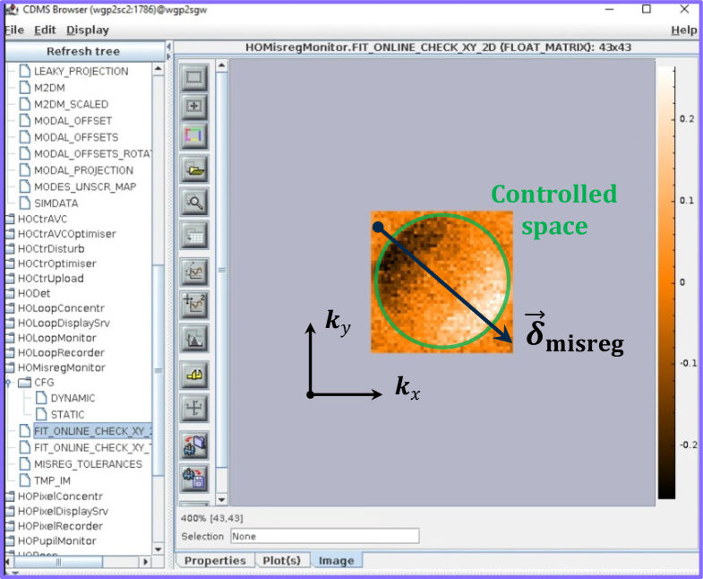
(a)	(b)	(c)

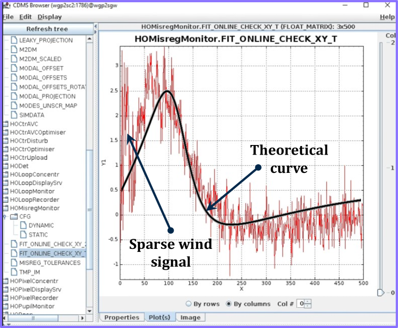
Figure 4: Monitoring and correcting the lateral error in the GPAO bench. Panel a: convergence of the corrective loop. Top: lateral error estimated by the proposed method. Bottom: absolute positioning of the WFS stage. Panels b,c: CDMS screenshots of the estimator sanity check outputs. Panel b: Map of the 2D coefficients $\tilde{\mathscr{C}}^{\text{2D}}$. Panel c: Curve of the temporal correlation $\tilde{\mathscr{C}}^{\text{t}}$ (red). The black curve is the theoretical correlation curve ${\boldsymbol{\mathscr{C}}}_{\!0}$ for ${{\boldsymbol{\delta}}}\rightarrow 0$.

First, it can be seen that the estimator found some lateral errors along the two axes, despite the WFS has been translated along a single axis. This is because there was an angle between the DM and the WFS, not lying in a Fried geometryFried:77. This angle is accounted for by the corrective loop.

Second, the amplitude estimated by the closed loop estimator was $\sim 12\,\%\Delta$, well below the $60\,\%\Delta$ theoretically injected. As discussed in depth in Berdeu:24_misreg, this is a known drawback of the closed loop estimator. Its sensitivity depends on the noise sources in the system, impacting the normalization in Eq. (9). It is nonetheless always smaller than one, ensuring the stability of the lateral error corrective loop.

As shown by the bottom panel of Fig. 4a, this corrective loop successfully converged. Bur there was a slight bias compared to the reference position. This reference was obtained with the phase plates stopped but inserted in the beam. They are known to introduce wobble in the system, adding an additional lateral error evolving with their rotation angle. The mentioned bias is considered to be within the margins of this wobble. It was thus considered that the estimator successfully converged without any strong bias induced by the frozen flow components of the turbulence.

In addition, the estimator has been integrated in SPARTA so that some sanity check outputs are published in its Configuration Data Management System (CDMS). Namely, the 2D map of the best fit of the coupling coefficients $\theta$:

$$\tilde{\mathscr{C}}^{\text{2D}}\left({{\boldsymbol{k}}}\right){}\triangleq{}\underset{\mathscr{C}_{\!}}{\text{argmin}}\;\sum_{f>0}\left(\tilde{\mathscr{C}}^{\text{cl}}\left({{\boldsymbol{k}}},f\right)-{\boldsymbol{\mathscr{C}}}_{\!0}\left(f\right)\mathscr{C}_{\!}\right)^{2}{}={}\frac{\sum_{f>0}\tilde{\mathscr{C}}^{\text{cl}}\left({{\boldsymbol{k}}},f\right){\boldsymbol{\mathscr{C}}}_{\!0}\left(f\right)}{\sum_{f>0}{\boldsymbol{\mathscr{C}}}_{\!0}^{2}\left(f\right)}\,,$$ (11)

shown in Fig. 4b, and the best fit of the correlation curves:

$$\tilde{\mathscr{C}}^{\text{t}}\left(f\right){}\triangleq{}\underset{\mathscr{C}_{\!}}{\text{argmin}}\;\sum_{{{\boldsymbol{k}}}\in\mathcal{K}^{\text{ctrl}}}\left(\tilde{\mathscr{C}}^{\text{cl}}\left({{\boldsymbol{k}}},f\right)-2\pi\mathscr{C}_{\!\,}{{\boldsymbol{k}}}^{T}\!\!\cdot\tilde{{{\boldsymbol{\delta}}}}\right)^{2}{}={}\frac{\sum_{{{\boldsymbol{k}}}\in\mathcal{K}^{\text{ctrl}}}\tilde{\mathscr{C}}^{\text{cl}}\left({{\boldsymbol{k}}},f\right){{\boldsymbol{k}}}^{T}\!\!\cdot\tilde{{{\boldsymbol{\delta}}}}}{\sum_{{{\boldsymbol{k}}}\in\mathcal{K}^{\text{ctrl}}}2\pi\left({{\boldsymbol{k}}}^{T}\!\!\cdot\tilde{{{\boldsymbol{\delta}}}}\right)^{2}}\,,$$ (12)

shown in Fig. 4c.

Looking at Fig. 4b, it appears that the map follows the expected ‘tip-tilt’ pattern from Eq. (5) according to the 2D spatial frequency. In addition, the correlation is limited to the space controlled by the AO system, delimited by the green circle (dictated by the number of controlled modes, namely 800 here, see Berdeu:24_misreg for more details).

Finally, the best fit of the temporal correlation curves of the command telemetry, shown in Fig. 4c, nicely matches the theoretical curve, in black. At low temporal frequencies, their is a corruption of the correlation signal by the wind. As expected, this effect remains sparse, limited to a narrow frequency range. It did not impact the quality of the convergence of the lateral error corrective loop.

3.2.2 First on-sky results

In the previous section, the closed loop estimator was tested against phase plates emulating frozen flow turbulence, the worst case offender for the method. In reality, atmospheric turbulence is more complex, potentially presenting several layers and characteristic wind speeds or coherence times that may impact the estimator performances. Before the upcoming commissioning of GRAVITY+, it was thus interesting to test the method on data acquired on-sky with other instruments.

The CHARA collaboration kindly shared data acquired during technical time (2023-10-16) from the E2 unit. An additional ‘Garching remote access facility’ (G-RAF) session (2024-05-28) on the GRAVITY/CIAO system, based on the soon to be decommissioned Multiple Application Curvature Adaptive OpticsArsenault:03_MACAO (MACAO), was also granted by the European Southern Observatory on the third telescope unit (UT3) of the Very Large Telescope (VLT).

The DMs of both systems own 60 actuators. Nonetheless, they do not lie on a Cartesian grid, as shown on Figs. 5a,b. As a consequence, the commands from the AO telemetry cannot be directly linked with a 2D representation. To overcome this issue, a low resolution projector, with $\sim 1.5$ pixel per actuator, was used to reshape the DM commands in 2D patterns, as presented in Figs. 5c,d.

	CHARA DM		MACAO DM
	Single actuator	Maximal projection	Single actuator	Maximal correlation
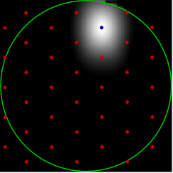
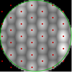
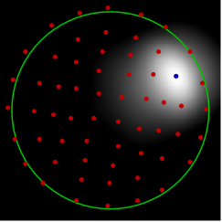
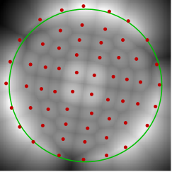
Influence function	(a1)	(b1)	(a2)	(b2)
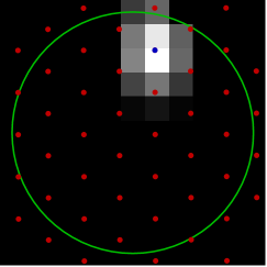
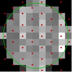
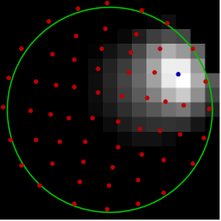
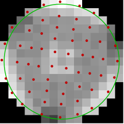
Command projector	(c1)	(d1)	(c2)	(d2)

Figure 5: Non-Cartesian grids of the CHARA (Panels 1) and GRAVITY/CIAO DM (Panels 2). Panels a,b: High resolution influence function and their maximal projection. Panels c,d: Low resolution model for the command 2D projection. Green circle: pupil edge. Colored dots: actuator position.

The main parameters impacting the correlation curves of the closed loop estimator are listed in Table 1. For each instrument, a batch of 2500 telemetry frames was used, corresponding to only $5\text{\,}\mathrm{s}$.

Table 1: Parameters of the CHARA and CIAO AO loops.

	CHARA	CIAO
Loop frequency $1/\tau^{\text{wfs}}$ ($\text{\,}\mathrm{H}\mathrm{z}$)	441	500
Loop gain $g^{\int}$	0.19	0.4
Number of controlled mode	41	45

The sanity check outputs of the closed loop estimator are given in Fig. 6. As for the results in the GPAO bench, the ‘tip-tilt’ pattern is nicely visible in the maps of the coupling coefficients $\tilde{\mathscr{C}}^{\text{2D}}$ and is well encompassed in the predicted controlled area, see Figs. 6a1,a2. Looking at the temporal correlation curves, see Figs. 6b1,b2, it first appears that the theoretical curves, in black, are different. This comes from the different gains of the AO loop used in each system. Despite the small number of actuators and controlled modes and the shortness of the gathered telemetry, the correlation signal is clear in the gray curves. Once filtered with a sliding windows, in red, the curve perfectly matches the prediction in the CHARA dataset. In the CIAO telemetry, the low frequencies are polluted by some wind signal.

CHARA telemetry		CIAO telemetry
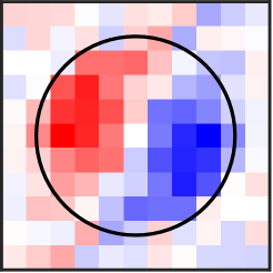
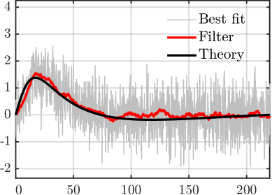
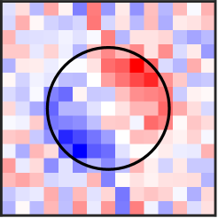
(a1)	(b1)	(a2)	(b2)
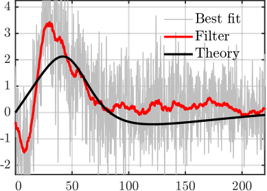
Spatial frequency ${{\boldsymbol{k}}}$	Frequency $f$ ($\text{\,}\mathrm{H}\mathrm{z}$)	Spatial frequency ${{\boldsymbol{k}}}$	Frequency $f$ ($\text{\,}\mathrm{H}\mathrm{z}$)

Figure 6: Sanity check outputs of the lateral error estimator with on-sky closed loop telemetry from CHARA (Panels 1) and GRAVITY/CIAO (Panels 2). Panels a: Map of the 2D coefficients $\tilde{\mathscr{C}}^{\text{2D}}$. The black circles encompass the spatial frequencies of the controlled space. Panels b: Curve of the temporal correlation $\tilde{\mathscr{C}}^{\text{t}}$ (gray). The black curve is the theoretical correlation curve ${\boldsymbol{\mathscr{C}}}_{\!0}$ for ${{\boldsymbol{\delta}}}\rightarrow 0$. The red curve is a mean filter of $\tilde{{\boldsymbol{\mathscr{C}}}}^{\text{t}}$ with a sliding window of $\pm 25$ data points.

To further investigate the impact of real turbulence wind on the closed loop estimator, known lateral shifts were introduced in the CIAO system, as shown in Fig. 7. The CIAO WFS was translated by steps of $25\text{\,}\mathrm{\SIUnitSymbolMicro m}$, up to $\pm 150\text{\,}\mathrm{\SIUnitSymbolMicro m}$, corresponding to an misalignment of $\pm 90\,\%\Delta$.

-90 %$\Delta$ offset	Reference CIAO position	+90 %$\Delta$ offset
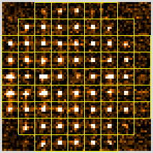
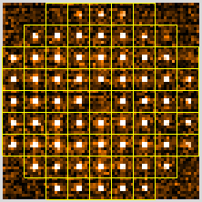
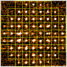
(a)	(b)	(c)

Figure 7: Application of different lateral offsets along the $x$-axis on the CIAO WFS stage. Loop closed on the VLT UT3 internal beacon inserting a neutral density filter in the beam.

The estimator was first tested on the beacon of the VLT UT3. To maximize the mis-registration signal, induced by the noise propagation through the AO loop, a neutral density filter was inserted in the beam. For each shift, $20\text{\,}\mathrm{s}$ of telemetry was recorded (10000 points). To get some statistics and assess the estimator covariance, 31 batches of 2500 consecutive frames every 250 telemetry frames were analyzed.

The results are shown in Fig. 8a. The bars indicate the $1\sigma$ error axes derived from the 2D covariances. It first appears that the estimated mis-registrations are rotated compared to the theoretical lateral shifts applied along the WFS $x$ and $y$-axes. This clocking is induced by the K-mirror position in-between the MACAO DM and the CIAO WFS. As mentioned above, the sensitivity of the closed loop estimator is not equal to unity and the comparison of its outputs with the injected shifts is not straightforward. To do so, the best linear transform linking the estimated mis-registrations $\tilde{{{\boldsymbol{\delta}}}}$ with their corresponding theoretical lateral shifts ${{\boldsymbol{\delta}}}^{\text{th}}$ was computed as follows:

$$(\widetilde{𝜹{}_0},\tilde{\rho },\tilde{\alpha })=\underset{𝜹{}_0,\rho ,\alpha }{\text{argmin}}\sum {}_{𝜹{}^{\text{th}}}(\widetilde{𝜹}(𝜹{}^{\text{th}})-\rho \times (𝜹{}_0+𝑹\left(\alpha \right)\times 𝜹{}^{\text{th}})){}^2,where𝑹\left(\alpha \right)istherotationmatrixofangle\alpha .InFig.\text{<a href="\#S3.F8" title="Figure 8In 3.2.2 First on-sky results ‣ 3.2 Experimental Results ‣ 3 Non-perturbative closed loop estimator ‣ Open loop calibration and closed loop non perturbative estimation of the lateral errors of an adaptive optics system: examples with GRAVITY+ and CHARA experimental data" class="ltx\_ref ltx\_font\_italic"><span class="ltx\_text ltx\_ref\_tag">8</span></a>}a,theestimatedlateralerrorswerethusscaledby1/\rho ,tobeputinregardstotheinjectedshiftsrotatedintheDMspaceby\alpha (blackdots).\text{Figure 8Figure 88Figure 8 \hspace{0.33em}\hspace{0.33em}8ComparisonontheVLT/UT3beaconoftheclosedloopestimator(blueandredalterna}$$ (13)