Convex Distillation: Efficient Compression of Deep Networks via Convex Optimization
Abstract
Deploying large and complex deep neural networks on resource-constrained edge devices poses significant challenges due to their computational demands and the complexities of non-convex optimization. Traditional compression methods such as distillation and pruning often retain non-convexity that complicates fine-tuning in real-time on such devices. Moreover, these methods often necessitate extensive end-to-end network fine-tuning after compression to preserve model performance, which is not only time-consuming but also requires fully annotated datasets, thus potentially negating the benefits of efficient network compression. In this paper, we introduce a novel distillation technique that efficiently compresses the model via convex optimization – eliminating intermediate non-convex activation functions and using only intermediate activations from the original model. Our approach enables distillation in a label-free data setting and achieves performance comparable to the original model without requiring any post-compression fine-tuning. We demonstrate the effectiveness of our method for image classification models on multiple standard datasets, and further show that in the data limited regime, our method can outperform standard non-convex distillation approaches. Our method promises significant advantages for deploying high-efficiency, low-footprint models on edge devices, making it a practical choice for real-world applications. We show that convex neural networks, when provided with rich feature representations from a large pre-trained non-convex model, can achieve performance comparable to their non-convex counterparts, opening up avenues for future research at the intersection of convex optimization and deep learning.
Knowledge Distillation, Non-Convex/Convex Optimization, Convex Neural Networks, Label-Free Training, Edge Machine Learning.
1 Introduction
Deep Neural Networks (DNNs) have become the cornerstone for a broad range of applications such as image classification, segmentation, natural language understanding and speech recognition (Rawat and Wang, 2017; Torfi et al., 2021; Alam et al., 2020; Sultana et al., 2020). The performance of these models typically scale with their size, width and architectural complexity, leading to the development of increasingly large models to achieve state-of-the-art results. However, this also necessitates significant computational, memory and energy resources to attain reasonable performance (Bianco et al., 2018; Rosenfeld, 2021); making their deployment impractical for resource-constrained edge devices – such as smartphones, microcontrollers, and wearable technology – which are of daily use (Ignatov et al., 2019; Anwar and Raychowdhury, 2020; Seng et al., 2023; Chen and Liu, 2021). Edge deep learning is crucial in these contexts to enable real-time processing, reduce latency, and ensure reliable operation without constant network connectivity (Kusupati et al., 2018; Tan and Le, 2019; Voghoei et al., 2018; Zaidi et al., 2022). Even in cases where such devices can make predictions by offloading the the computations to large models on cloud servers, developing memory and compute efficient models is still advantageous as it reduces network bandwidth usage, lowers operational costs, and allows cloud services to serve more clients within the same resource constraints.
Non-convex optimization, which forms the bedrock of training DNNs, poses significant theoretical and practical challenges. Finding the global minimum can be NP-hard in the worst case and the optimization landscape is riddled with local minima (Yao, 1992; Bartlett and Ben-David, 1999) and saddle points (Dauphin et al., 2014), making it difficult to guarantee convergence to a global optimum (Choromanska et al., 2015). Moreover, even training these models in a distributed manner on multiple GPUs can take days or weeks to complete. Convex optimization, on the other hand, is well-studied with strong theoretical guarantees and efficient algorithms (Boyd and Vandenberghe, 2004). While there are recent works that show one can reformulate the optimization of certain classes of non-convex NNs as convex problems (Pilanci and Ergen, 2020a; Ergen et al., 2022a), convex models are generally considered less expressive than their non-convex counterparts (Guss and Salakhutdinov, 2019; Scarselli and Chung Tsoi, 1998) and have been overshadowed by the success of deep learning in recent years.
Although large non-convex DNNs possess immense expressive power, they often contain redundant weights that contribute little to the overall performance in downstream tasks (Frankle and Carbin, 2019; Han et al., 2015). This phenomenon called Implicit Bias has been well established in both theory and practice (Soudry et al., 2024; Chizat and Bach, 2020; Morwani et al., 2023; Shah et al., 2020). Additionally, while DNNs have the capacity to memorize the training dataset, they often end up learning basic solutions that generalize well to test datasets (Zhang et al., 2021). Both of these observations motivate using smaller, compressed models that eliminate unnecessary parameters while achieving comparable performance. Common techniques for model compression include network pruning (Han et al., 2015), low-rank approximation (Denil et al., 2013), and quantization (Gong et al., 2014). However, these methods often significantly degrade performance of the resulting model unless supplemented by another round of extensive fine-tuning on the labeled training data post-compression, which may not be feasible in many practical scenarios. Knowledge distillation (KD) is a promising alternative that enables a smaller student model to learn from a larger teacher model (Hinton et al., 2015) by training the student to mimic the outputs or intermediate representations of the teacher by matching certain statistical metrics between the two models. While KD can significantly enhance the performance of the student model, it often still requires fine-tuning the student model on labeled data in conjunction with the activation matching objective, limiting its applicability in situations where labeled data or compute is scarce or unavailable.
In this paper, we bridge the gap between the non-convex and convex regimes by demonstrating that convex neural network architectures can achieve performance comparable to non-convex models for downstream tasks when leveraging rich feature representations. To demonstrate this, we focus on the model compression via KD framework and propose a novel approach that compresses non-convex DNNs via convex optimization. Our approach replaces the original complex non-convex layers in the teacher module with simpler layers having convex gating functions in the student module. By matching the activation values between the teacher and student modules, we eliminate the need for post-compression fine-tuning on labeled data, making our method suitable for deployment in environments where labeled data is scarce. Our method not only maintains the performance of the original large model, but also capitalizes on the favorable optimization landscape of convex models. This enables users to employ a range of highly efficient and specialized convex solvers tailored to their resource requirements, resulting in faster convergence and the potential for on-device learning using online data—a significant advantage for edge devices with limited computational resources.
Summary of our Contributions:
Efficient Convex-based Distillation and Deployment:
We introduce a novel knowledge distillation approach that leverages convex neural network architectures to compress DNNs. By replacing non-convex layers with convex gating functions in the student module, we exploit the well-understood theoretical foundations and efficient algorithms available in the convex optimization literature. Our method achieves better performance than non-convex distillation approaches even when using the same optimizer due to a more favorable optimization landscape. Moreover, the convexity of the student module allows us to employ faster and more specialized convex optimization algorithms, leading to accelerated convergence and reduced computational overhead. This facilitates real-time execution and on-device learning on resource-constrained edge devices.
Label-Free Compression Without Fine-Tuning:
Our method focuses on activation matching between a larger non-convex teacher module and a smaller convex student module on unlabeled data. We show that for many real-world tasks, convex distillation in itself sufficient for the resulting model to perform well at inference time, eliminating the need for any fine-tuning on labeled data after compression. This makes our approach applicable in scenarios where labeled data is scarce.
Bridging the Non-Convex and Convex Regimes:
To the best of our knowledge, this is the first work that marries the expressive representational power of non-convex DNNs with the theoretical and computational advantages of convex architectures. Our empirical results on real-world datasets demonstrate that convex student models can achieve high compression rates without sacrificing accuracy, often significantly outperforming non-convex compression methods in low-sample and high-compression regimes. This provides strong empirical evidence supporting the viability of convex neural networks when leveraging rich features from pre-trained non-convex teacher models, opening new avenues for research at the intersection of deep learning and convex optimization.
2 Other Related Work
Knowledge distillation (KD) has been a pivotal technique for compressing DNNs by transferring knowledge from a large teacher model to a smaller student model. In this section, we discuss several related methods, highlighting their advantages and the limitations that our approach addresses.
In their seminal work, Romero et al. (2015) introduced FitNets, where a thin and wide student model mimics the behavior of a larger teacher models by matching intermediate representations. By aligning the activations of a guided layer in the student with the outputs of the hint layer in the teacher, they prevent over-regularization and allow effective learning of the student on the training dataset. Since Fitnets were introduced, many methods have proposed modifications on top of them, such as designing new types of features (Kim et al., 2020; Srinivas and Fleuret, 2018), changing the teacher/student architectures (Lee et al., 2022) and distilling across multiple layers (Chen et al., 2021). However, nearly all of them require access to labeled training data for fine-tuning, and the optimization process remains non-convex, making convergence guarantees difficult.
Tung and Mori (2019) proposed a method inspired by contrastive learning: preserve the relative representational structure of the data in the student model by ensuring that input pairs that produce similar (or dissimilar) activations in the teacher model produce similar (or dissimilar) activations in the student network. This approach improves generalization but is computationally expensive, especially with large batch, due to the quadratic complexity of producing pairwise comparisons. Further, training objective is a weighted sum of cross entropy loss between the pairwise similarity activations and a fine-tuning loss on the training data, necessitating access to labeled training data.
Heo et al. (2018) introduced an activation transfer loss that minimizes the differences in boolean activation patterns instead. This addresses the issue of the loss emphasizing samples with large activation differences while underweighting those with small yet significant differences, which can make it difficult to differentiate between weak and zero responses. However, their method involves optimizing a computationally intensive non-convex objective function.
Recent advances have explored KD without access to the original training data. Yin et al. Raikwar and Mishra (2022) proposed generating synthetic data by sampling from a Gaussian distribution and adjusting the distributions within the teacher model’s hidden layers. While this allows for label-free distillation, the synthetic data may not capture the complexity of real data distributions. Additionally, their method relies on specific implementations of BatchNorm layers in the teacher model and focuses on label-free distillation without addressing the challenges of non-convex optimization. Since our method is only concerned with intermediate activations and not the input-output nature of samples, it is also directly applicable on the synthetic data generated by their approach.
3 Preliminaries
3.1 Notation
denotes the set . For a matrix , denotes row of . For a vector , denotes element of . We sometimes use to denote an indexed vector; in this case denotes the element of . denotes euclidean norm of a vector. For a sparse vector , we define the support as . We use to denote the identity matrix and to be the indicator function. For a matrix , vectorizes the matrix by stacking columns sequentially. Unless stated otherwise, is the number of samples in the training dataset and is the dimenionality of the input samples.
3.2 Convex Neural Networks
Pilanci and Ergen (2020b) prove that training a two-layer fully-connected NNs with ReLU activations can be reformulated as standard convex optimization problems. This result is important because it allows us to leverage convex optimization techniques while retaining the expressive power of DNNs.
Theorem 1 (Convex equivalence for ReLU networks).
Let be a data matrix and the associated scalar targets. The two-layer ReLU neural network can then be expressed as:
where , are the weights of the first and second layers, is the number of hidden units, and is the ReLU activation. Then, the optimal weights and that minimize the convex loss function with a - regularization penalty can be obtained by first solving the following optimization problem:
| (1) |
where sub-sampling is over neurons , is the set of hyperplane arrangement patterns i.e. the set of activation patterns of neuron in the hidden layer for a fixed and is a convex cone; and setting
for some s.t. and .
This leads to solving a practically intractable quadratic program for large as where . Instead, we solve an unconstrained version of the above problem:
Theorem 2 (Convex equivalence for GReLU networks).
Let and denote the gated ReLU (GReLU) activation function. Then the model
is a GReLU network where each is a fixed gate. Let such that and . Then, the optimal weights and for the regularized convex loss function can be obtained by solving the following convex optimization problem:
| (2) |
and setting .
The main difference between Theorem 2 and Theorem 1 is the activation function. Using fixed gates , the activation function is linear in and the non-linearity introduced by the gating matrix is fixed with respect to the optimization variables and . Since each term in the optimization problem involves a product of and , it is bilinear in and . At first glance, this may suggest that the optimization is non-convex as bilinear functions are generally non-convex. However, in this specific case, we can transform the problem into a convex one through reparameterization (specifically, set ). (For details, see Section A.1)
One can show that the solutions to the optimization problems in Theorems 2 and 1 are guaranteed to approximate each other if the number of samples is sufficiently large. Kim and Pilanci (2024) show that under certain assumptions on the input data Gaussian gates are sufficient
for local gradient methods to converge with high probability to a stationary point that is relative approximation of the global optimum of the non-convex problem. Lastly, note that the above theorems are hold only for scalar outputs, and by extension, binary classification problems. Mishkin et al. (2022) extend the above theorems to vector valued outputs by using a one-vs-all approach for each entry in the output vector and the following reformulation:
Theorem 3 (Convex equivalence for vector output networks).
Let be the model output dimension, the associated targets, and the weights of the second layer. Then,
A. The two-layer ReLU neural network with vector output can be expressed as:
and the optimal weights and can recovered by solving the following one-vs-all convex optimization problem:
| (3) | ||||
| (4) |
B. The two-layer GReLU neural network with vector output and the corresponding convex optimization problem can be expressed similarly to the above except with the change that is replaced by in the statements and the constrained nuclear norm penalty being replaced with a standard nuclear norm penalty.
4 Approach: Distillation via Activation Matching
4.1 Distilling Vision Classification Models using Convex Networks
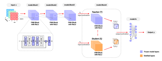
Consider a Model that has been trained on a dataset drawn from the data distribution . As discussed previously, one common way to compress the model size is to prune the architecture, say via magnitude thresholding, and get rid of redundant or non-contributing weights across the DNN layers. In our case, we will focus on compressing the upper blocks of the model where each block itself can comprise of multiple layers of varying kinds such as Convolution, Batchnorm, Pooling, MLP, etc. We refer to the (original) block that we want to compress as Teacher () and the post-distillation resulting block to be Student (). We use these terms to conceptually relate to the nomenclature prevalent in distillation literature.
Let the set of input activations just before the Teacher block generated by inferencing the with a single pass over a dataset be . Let the output functions of and blocks be denoted by and respectively. Then we can distill the knowledge of onto by minimizing the following activation matching objective:
| (5) |
i.e., we enforce the new block to learn the input-output activation value mapping over the data distribution. In practice however, we find the optimal weights of by solving the following ERM:
| (6) |
Once we have trained with activation matching, we simply swap out with . Post replacement, we do not perform any fine-tuning of any other parameter of the model using the training dataset. In fact, all other layers in the model are kept frozen with their original weights and we directly perform test time inference (see Figure 1). Note how this approach is label free as there is no explicit dependency on the output in the optimization problem. The only design constraint for is that the dimensions of input-output of should exactly match the dimensions for the input-output activations of the original block , i.e., .
Unlike other distillation methods that preserve non-convexity our approach gets rid of any non-convexity in the constituent layers of . For instance, consider Figure 1 where the number of parameters in increase significantly as we move from Block #1 to Block #4 ((see Table 1). Block #4 of Resnet18 alone contributes roughly 70% of the total model size and compressing it to -th its size compresses the overall model by . Each block in Resnet18 has multiple CNN, Batchnorm, AvgPool, and ReLU layers which results in sophisticated non-convex model with high expressivity.
| Resnet Block | Input Dim | Output Dim | #Params | #Params | Sparsity | |
|---|---|---|---|---|---|---|
| Block | Overall | |||||
| Block1 | 147,968 | 73,328 | 0.495 | 0.994 | ||
| Block2 | 525,568 | 164,608 | 0.313 | 0.969 | ||
| Block3 | 2,099,712 | 656,896 | 0.313 | 0.8765 | ||
| Block4 | 8,393,728 | 1,312,768 | 0.156 | 0.394. | ||
We now describe how to construct a convex . Note that AvgPool is a linear operator and therefore preserves convexity. Furthermore, training regularized ReLU networks with Batchnorm can be reformulated as a finite-dimensional convex problem (Ergen et al., 2022b). Therefore, a composition of these operations is still a convex operation. Now, the non-convexity of stems primarily from the composition of multiple ReLU layers inside the block. Consider the simplified functional expression of the teacher module where we omit all the Batchnorm and AvgPool layers, , where
| (7) |
i.e., is the composition of smaller 2-CNN layer ReLU networks () and is a fixed number that depends on actual the model architecture.
To distill this via convex models, we will set to be a 3-CNN layer block such that:
| (8) |
Remarks on the convexity of : In Sahiner et al. , it is shown that the above architecture corresponds to the Burer-Monteiro factorization of the convex NN objective in equation 4 for vector outputs, and all local minima are globally optimal (see Theorem 3.3 in Sahiner et al. ). Also note (i) is a boolean mask that masks out the corresponding entries in the outputs of . Since the mask values are , no gradient is back-propagated to the parameters of , it does not contribute any effective parameter to the model size. Alternatively, we can mask out using fixed boolean masks. (ii) is the main output generating layer. iii) is filter which is used to ensure that the shapes of and match. Observe that it was not necessary for in this example to be composed of CNN layers. In fact, any block that matches input-output activation dimensions, irrespective of the architecture design, could have been used.
4.2 Accelerating Distillation using Convex Solvers
In the previous subsection, we discussed how one can compress a large model by distilling its large non-convex modules into smaller convex modules. When the optimization problem is convex, saddle points and non- global minima do not exist, facilitating faster convergence even with momentum-based optimization methods (Assran and Rabbat, 2020). Therefore, convex formulations can accelerate the test-time fine-tuning of the compressed model in presence of new data when compared to their non-convex counterparts. To push these benefits to the limit, we employ fast convex solvers.
Given that the only constraint on is matching the shape of the input-output activations with , we draw inspiration from the work of Mishkin et al. (2022) on 2-layer convex and non-convex MLP models, and setup as a 2-layer GReLU MLP along the lines of Theorems 2 and 3. While we demonstrate the effects of convexity when using standard optimtizers like Adam (Paszke et al., 2019) to train , solving the resulting group lasso regression can be more efficiently handled by specialized convex optimization algorithms. The SCNN Python library 111https://pypi.org/project/pyscnn/ provides fast and reliable algorithms for convex optimization of two-layer neural networks with ReLU activation functions. Specifically, it implements the R-FISTA algorithm, an improved version of the FISTA algorithm (Beck and Teboulle, 2009), which combines line search, careful step-size initialization, and data normalization to enhance convergence. We utilized R-FISTA as the convex solver in this paper.
4.3 Improving Convex Solvers Via Polishing
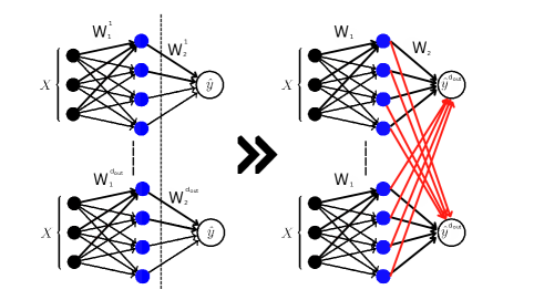
While the SCNN package is optimized for scalar outputs, it handles vector output optimization problems by adopting a one-vs-all approach for each output dimension, i.e. return where each . This inhibits any information sharing between the weight matrices corresponding to different nodes in the multi-dimensional model output. To overcome this, we can explicitly impose information sharing between the weight matrices s, and in the process arguably obtain a better solution for an even sparse solution for , leading to possibility of further model compression. One way to do this is to freeze the stacked matrices computed by SCNN and recompute (initialized with obtained from SCNN) but with a group elastic constraint on rows of (See Appendix A.2 for the mathematical setup). Using a group elastic constraint on the "shared" regressor encourages using features from different ’s and therefore acts as a feature selector. This essentially translates to zeroing-out entire columns of and compress the model further. To implement this, we use the open source python package Adelie222https://jamesyang007.github.io/adelie/index.html that can solve the group elastic regression problem in a heavily parallelized manner.
5 Experiments
In this section, we conduct an empirical study with the following goals: a) to demonstrate that using convex neural networks and distilling via convex optimization performs as well, if not better than, non-convex distillation; and b) to show that our approach generalizes well in low-sample regime and that using convex solvers is an order of magnitude faster than training non-convex models. We consider the following baselines: 1) Full Fine-tuned Model (FFT): The original full fine-tuned model () undergoing compression, 2) Convex-Gated (): learns a compressed block with convex-gating activations, 3) Non-Convex () learns a non-convex compressed block with ReLU activation, and 4) Pruning : prunes the weights in . We set the compressed blocks and s.t. they have the same parameter count as in . This enables a fair performance comparison between each of the distillation methods. We use SVHN (Netzer et al., 2011), CIFAR10 (Krizhevsky and Hinton, 2009), TinyImagenet (Le and Yang, 2015), and Visual Wake Words (Chowdhery et al., 2019) datasets to establish the validity of our approach.
5.1 Convex Distillation of CNN Blocks using standard optimizers
First, we measure the performance of KD based compressed blocks, as described in Section 4.1, by comparing the effects of convexity and non-convexity in the design of :
and optimizing the Mean Squared Error as in equation 6 using Adam Optimizer. For both methods, we incorporate BatchNorm and AvgPool layers in the architecture since they preserve convexity and lead to improved results. To obtain different compression rates when distilling the blocks (reported as X times the original model size), we vary the number of filters of in from 1 to 512 in multiples of 2. Then, for a fair comparison, we adjust the number of filters in the CNN layers of to match the parameter count of . Since provides only a boolean mask and has no gradient back-propagated to it, and is a convolution layer, typically for the same number of filters, .
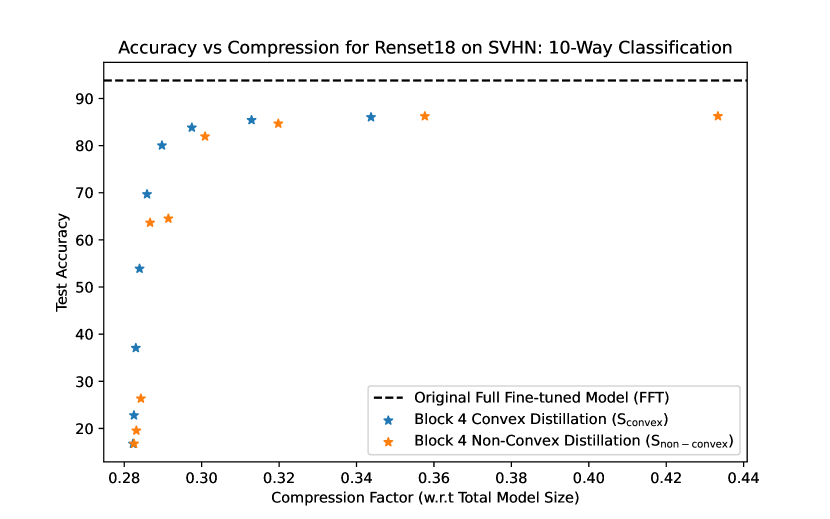
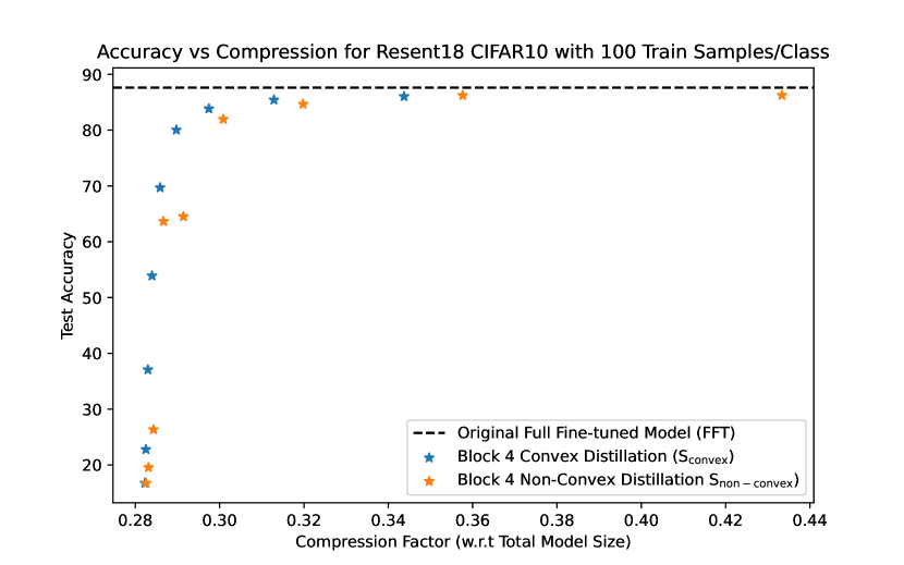
Figure 3(a) demonstrates the test-set accuracy versus total model size as we double the number of filters in the compressed Block 4 of ResNet-18 on the SVHN dataset. Note that in the extremely low model size regime (number of filters = 1, 2, 4, 8, 16), significantly outperforms . On the CIFAR10 dataset, we also compress Block 3 along with Block 4 of Resnet18 by varying the number of filters in multiples of 2 from 1 to 512. We compare the performance of both and against magnitude-based pruning, where we preserve a certain percentage of weights based on their magnitude and zero out the remaining entries in the weight matrices. We then swap different combinations of the compressed versions of Blocks 3 and 4 into the original model.
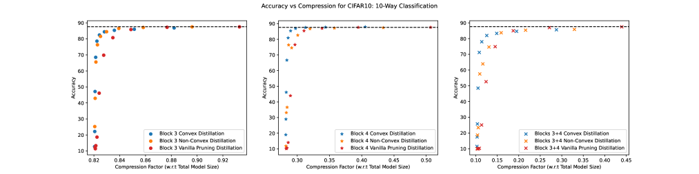
Figure 4 demonstrates the efficacy of our v/s on CIFAR10 dataset. All subplots compare the test set accuracies without any post-compression training or fine-tuning on the labeled dataset. Note that utilizing the compressed versions for both Blocks 3 and 4 leads to 10x compression compared to the original fine-tuned model in size, with no significant drop in performance on the full test set. The figure shows that while both and perform well when distilling only Block 3, outperforms when distilling Block 4, especially at higher compression rates. This becomes more evident as we use different compressed combinations of both Blocks 3 & 4.
Next, we consider the performance of and in the low-sample regime. We train both and (compressing Block 4) using only 100 randomly selected training samples per class and compare their performance on the full dataset ( 25K samples) against the Resnet18 model fine-tuned on original training dataset. Figure 3(b) shows that performance gap between and is even more prominent in this data-scarce regime.
So far, we have used the Adam optimizer to train both the convex and non-convex compressed blocks in these experiments. In the subsequent experiments, we leverage fast convex solvers for distillation.
5.2 Fast Distillation Using Convex Solvers
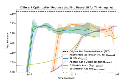
To demonstrate the superiority of convex distillation over non-convex distillation in low-resource settings, we consider the 2 layer MLP formulation of (GReLU activation) and (ReLU activation) described in Section 4.2. We use the SCNN library to solve the activation-matching problem for and the Adam optimizer for the block. The time budget for Adam is set slightly higher than that used by SCNN for a fair comparison. Recall that having a convex optimization problem for gives us the liberty to choose any convex solver, which requires minimal hand-tuning of hyperparameters. Figure 5 compares different convex solvers when distilling a Resnet18 model fine-tuned on a binary classification task in the TinyImageNet Dataset (german shephard v/s tabby cat) into perform at test time. In this Dataset, we have 500 training and 100 test samples per class, representing a data-scarce regime. For distilling to , we use both full-batch and mini-batch training using Adam. The experiment is repeated over 10 different seeds, and we plot the error curves for each method, with the solid line representing the mean and the shaded region indicating twice the standard deviation. The plot shows that RFISTA and Approximate Cone Decomposition are superior among the convex solvers. In contrast, both versions of Adam-trained non-convex models take nearly one-two orders of more time to reach the performance achieved by the convex solvers.
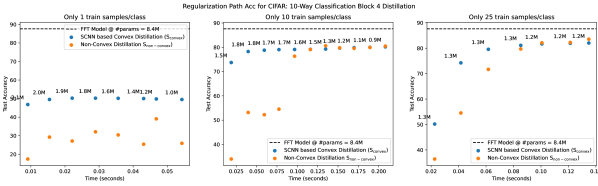
Since SCNN solves a one-vs-all problem for vector outputs, for the 10-way classification problem of CIFAR10, we set the hidden dimension of the network to be , determine the total number of non-zero entries in the weight matrices computed by SCNN (using the RFISTA solver) and use that to set the hidden layer size of the non-convex block. For an elaborate comparison between the two methods, at each point of the regularization path computed by SCNN, we track the the time required by it to solve the activation matching problem and use that as a time budget for the Adam-based training. We also impose constraints on the available number of training samples and report the test set accuracy of each method after swapping the distilled blocks back into the original model. Figure 6 shows the experiment results when we try to distill Block 4 from it’s original 8M parameter count to 1M at different training samples/class configurations. Note how in extreme labeled training data scarce settings, convex distillation performs far better than non-convex distillation.
5.3 Distillation via Proximal Gradient Methods followed by polishing
One may notice in Figure 6 that as we relax the constraints on the training time and the number of training samples available per class, non-convex NN seems to catch up to convex NN distillation.
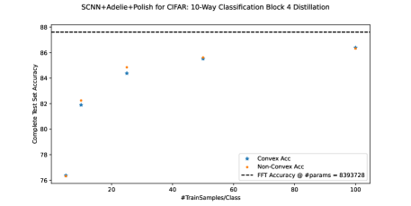
One key reason is that SCNN solves a one-vs-all problem which inhibits any information sharing between the weight matrices corresponding to different nodes in the multi-dimensional model output. To overcome this, we recompute by explicitly imposing information sharing between the constituent weight matrices (See Section 4.3). By obtaining a shared , we recover any performance lost due to additional compression by polishing and resolving a regularized linear regression problem. Figure 7 shows that even for relaxed resource constraints, convex optimization based distillation performs at least as good as with Adam-based non-convex block distillation. We believe that here convex distillation approach would outperform non-convex distillation if comprised of CNN layers instead of linear layers. Since SCNN only solves the training of 2-layer MLPs, we are constrained by the types of experiments we can do.
5.4 Beyond Distillation: End-To-End Fine-tuning of Convex Architectures
| Back-Bone | Classification Head | Accuracy |
|---|---|---|
| Frozen | Convex | 81.36 |
| Frozen | Non-Convex | 80.84 |
| Trainable | Convex | 83.47 |
| Trainable | Non-Convex | 83.42 |
As an ablation experiment, we study how convexity affects the fine-tuning of DNNs on labeled training datasets. Visual Wake Words is a benchmark dataset derived from COCO Lin et al. (2015) that assesses the performance of tiny vision models at the microcontroller scale (memory footprint of less than 250KB). For our experiment, we consider the Person/Not Person task, where the vision model determines whether a person is present in the image. There are a total of 115K images in the training and validation dataset 8k images in the test dataset. This task serves various edge machine learning use cases, such as in smart homes and retail stores, where we wish to detect the presence of specific objects of interest without a high inference cost. Using the ImageNet pre-trained MobileNet V3 model (Howard et al., 2019) as our base model, we preserve its back-bone upto the fourth layer and replace all the subsequent layers with a smaller architecture as the classification head. The classification head can be either convex or non-convex, as described in the previous experiments. We also consider scenarios where the back-bone is either kept frozen or trainable. We then fine-tune the resulting model on the COCO dataset with Adam on Cross-Entropy Loss, and report the Test Accuracy in Table 2.
When the back-bone is frozen, convex classification head performs noticeably better than its non-convex counterpart. This scenario represents a realistic situation where end-to-end fine-tuning of large models (e.g., large language models (LLMs) or vision-language models (VLMs)) can be prohibitively expensive for downstream tasks due to computational constraints. When the back-bone is trainable, i.e. all the parameters of the combined model can be updated during fine-tuning, using a convex head is very slightly better or nearly the same as a non-convex head. This experiment shows promise that convex NN architectures are good candidates for DNN applications beyond just distillation.
6 Conclusions
In this paper, we have introduced a novel approach that bridges the non-convex and convex regimes by combining the representational power of large non-convex DNNs with the favorable optimization landscape of convex NNs. Our experiments show that the disillation via convex architectures performs at least as good as prevalent non-convex distillation methods. Furthermore, our approach successfully distill models in a completely label-free setting without requiring any post-compression fine-tuning on the training data. This work opens new avenues for deploying efficient, low-footprint models on resource-constrained edge devices with on-device learning using online data. Future work could focus on developing convex optimization methods to directly solve for optimal weights without resorting to a one-vs-all setting for multi-dimensional outputs. Additionally, exploring applications in other domains, such as natural language processing and generative models, could further validate and expand the applicability of our approach.
References
- Rawat and Wang (2017) Waseem Rawat and Zenghui Wang. Deep convolutional neural networks for image classification: A comprehensive review. Neural Computation, 29(9):2352–2449, 2017. doi: 10.1162/neco_a_00990.
- Torfi et al. (2021) Amirsina Torfi, Rouzbeh A. Shirvani, Yaser Keneshloo, Nader Tavaf, and Edward A. Fox. Natural language processing advancements by deep learning: A survey, 2021. URL https://arxiv.org/abs/2003.01200.
- Alam et al. (2020) M. Alam, M.D. Samad, L. Vidyaratne, A. Glandon, and K.M. Iftekharuddin. Survey on deep neural networks in speech and vision systems. Neurocomputing, 417:302–321, 2020. ISSN 0925-2312. doi: https://doi.org/10.1016/j.neucom.2020.07.053. URL https://www.sciencedirect.com/science/article/pii/S0925231220311619.
- Sultana et al. (2020) Farhana Sultana, Abu Sufian, and Paramartha Dutta. Evolution of image segmentation using deep convolutional neural network: A survey. Knowledge-Based Systems, 201-202:106062, 2020. ISSN 0950-7051. doi: https://doi.org/10.1016/j.knosys.2020.106062. URL https://www.sciencedirect.com/science/article/pii/S0950705120303464.
- Bianco et al. (2018) Simone Bianco, Remi Cadene, Luigi Celona, and Paolo Napoletano. Benchmark analysis of representative deep neural network architectures. IEEE Access, 6:64270–64277, 2018. doi: 10.1109/ACCESS.2018.2877890.
- Rosenfeld (2021) Jonathan S. Rosenfeld. Scaling laws for deep learning, 2021. URL https://arxiv.org/abs/2108.07686.
- Ignatov et al. (2019) Andrey Ignatov, Radu Timofte, Andrei Kulik, Seungsoo Yang, Ke Wang, Felix Baum, Max Wu, Lirong Xu, and Luc Van Gool. Ai benchmark: All about deep learning on smartphones in 2019. In 2019 IEEE/CVF International Conference on Computer Vision Workshop (ICCVW), pages 3617–3635, 2019. doi: 10.1109/ICCVW.2019.00447.
- Anwar and Raychowdhury (2020) Aqeel Anwar and Arijit Raychowdhury. Autonomous navigation via deep reinforcement learning for resource constraint edge nodes using transfer learning. IEEE Access, 8:26549–26560, 2020. doi: 10.1109/ACCESS.2020.2971172.
- Seng et al. (2023) Kah Phooi Seng, Li-Minn Ang, Eno Peter, and Anthony Mmonyi. Machine learning and ai technologies for smart wearables. Electronics, 12(7), 2023. ISSN 2079-9292. doi: 10.3390/electronics12071509. URL https://www.mdpi.com/2079-9292/12/7/1509.
- Chen and Liu (2021) Xing Chen and Guizhong Liu. Energy-efficient task offloading and resource allocation via deep reinforcement learning for augmented reality in mobile edge networks. IEEE Internet of Things Journal, 8(13):10843–10856, 2021. doi: 10.1109/JIOT.2021.3050804.
- Kusupati et al. (2018) Aditya Kusupati, Manish Singh, Kush Bhatia, Ashish Kumar, Prateek Jain, and Manik Varma. Fastgrnn: A fast, accurate, stable and tiny kilobyte sized gated recurrent neural network. In S. Bengio, H. Wallach, H. Larochelle, K. Grauman, N. Cesa-Bianchi, and R. Garnett, editors, Advances in Neural Information Processing Systems, volume 31. Curran Associates, Inc., 2018. URL https://proceedings.neurips.cc/paper_files/paper/2018/file/ab013ca67cf2d50796b0c11d1b8bc95d-Paper.pdf.
- Tan and Le (2019) Mingxing Tan and Quoc Le. EfficientNet: Rethinking model scaling for convolutional neural networks. In Kamalika Chaudhuri and Ruslan Salakhutdinov, editors, Proceedings of the 36th International Conference on Machine Learning, volume 97 of Proceedings of Machine Learning Research, pages 6105–6114. PMLR, 09–15 Jun 2019. URL https://proceedings.mlr.press/v97/tan19a.html.
- Voghoei et al. (2018) Sahar Voghoei, Navid Hashemi Tonekaboni, Jason G. Wallace, and Hamid R. Arabnia. Deep learning at the edge. In 2018 International Conference on Computational Science and Computational Intelligence (CSCI), pages 895–901, 2018. doi: 10.1109/CSCI46756.2018.00177.
- Zaidi et al. (2022) Syed Ali Raza Zaidi, Ali M. Hayajneh, Maryam Hafeez, and Q. Z. Ahmed. Unlocking edge intelligence through tiny machine learning (tinyml). IEEE Access, 10:100867–100877, 2022. doi: 10.1109/ACCESS.2022.3207200.
- Yao (1992) Xin Yao. Finding approximate solutions to np-hard problems by neural networks is hard. Information Processing Letters, 41(2):93–98, 1992. ISSN 0020-0190. doi: https://doi.org/10.1016/0020-0190(92)90261-S. URL https://www.sciencedirect.com/science/article/pii/002001909290261S.
- Bartlett and Ben-David (1999) Peter Bartlett and Shai Ben-David. Hardness results for neural network approximation problems. In Paul Fischer and Hans Ulrich Simon, editors, Computational Learning Theory, pages 50–62, Berlin, Heidelberg, 1999. Springer Berlin Heidelberg. ISBN 978-3-540-49097-5.
- Dauphin et al. (2014) Yann Dauphin, Razvan Pascanu, Caglar Gulcehre, Kyunghyun Cho, Surya Ganguli, and Yoshua Bengio. Identifying and attacking the saddle point problem in high-dimensional non-convex optimization, 2014. URL https://arxiv.org/abs/1406.2572.
- Choromanska et al. (2015) Anna Choromanska, Mikael Henaff, Michael Mathieu, Gérard Ben Arous, and Yann LeCun. The loss surfaces of multilayer networks, 2015. URL https://arxiv.org/abs/1412.0233.
- Boyd and Vandenberghe (2004) Stephen Boyd and Lieven Vandenberghe. Convex Optimization. Cambridge University Press, 2004.
- Pilanci and Ergen (2020a) Mert Pilanci and Tolga Ergen. Neural networks are convex regularizers: Exact polynomial-time convex optimization formulations for two-layer networks. In Hal Daumé III and Aarti Singh, editors, Proceedings of the 37th International Conference on Machine Learning, volume 119 of Proceedings of Machine Learning Research, pages 7695–7705. PMLR, 13–18 Jul 2020a. URL https://proceedings.mlr.press/v119/pilanci20a.html.
- Ergen et al. (2022a) Tolga Ergen, Behnam Neyshabur, and Harsh Mehta. Convexifying transformers: Improving optimization and understanding of transformer networks, 2022a. URL https://arxiv.org/abs/2211.11052.
- Guss and Salakhutdinov (2019) William H. Guss and Ruslan Salakhutdinov. On universal approximation by neural networks with uniform guarantees on approximation of infinite dimensional maps, 2019. URL https://arxiv.org/abs/1910.01545.
- Scarselli and Chung Tsoi (1998) Franco Scarselli and Ah Chung Tsoi. Universal approximation using feedforward neural networks: A survey of some existing methods, and some new results. Neural Networks, 11(1):15–37, 1998. ISSN 0893-6080. doi: https://doi.org/10.1016/S0893-6080(97)00097-X. URL https://www.sciencedirect.com/science/article/pii/S089360809700097X.
- Frankle and Carbin (2019) Jonathan Frankle and Michael Carbin. The lottery ticket hypothesis: Finding sparse, trainable neural networks, 2019. URL https://arxiv.org/abs/1803.03635.
- Han et al. (2015) Song Han, Jeff Pool, John Tran, and William J. Dally. Learning both weights and connections for efficient neural networks, 2015. URL https://arxiv.org/abs/1506.02626.
- Soudry et al. (2024) Daniel Soudry, Elad Hoffer, Mor Shpigel Nacson, Suriya Gunasekar, and Nathan Srebro. The implicit bias of gradient descent on separable data, 2024. URL https://arxiv.org/abs/1710.10345.
- Chizat and Bach (2020) Lenaic Chizat and Francis Bach. Implicit bias of gradient descent for wide two-layer neural networks trained with the logistic loss, 2020. URL https://arxiv.org/abs/2002.04486.
- Morwani et al. (2023) Depen Morwani, Jatin Batra, Prateek Jain, and Praneeth Netrapalli. Simplicity bias in 1-hidden layer neural networks. In A. Oh, T. Naumann, A. Globerson, K. Saenko, M. Hardt, and S. Levine, editors, Advances in Neural Information Processing Systems, volume 36, pages 8048–8075. Curran Associates, Inc., 2023. URL https://proceedings.neurips.cc/paper_files/paper/2023/file/196c4e02b7464c554f0f5646af5d502e-Paper-Conference.pdf.
- Shah et al. (2020) Harshay Shah, Kaustav Tamuly, Aditi Raghunathan, Prateek Jain, and Praneeth Netrapalli. The pitfalls of simplicity bias in neural networks. In H. Larochelle, M. Ranzato, R. Hadsell, M.F. Balcan, and H. Lin, editors, Advances in Neural Information Processing Systems, volume 33, pages 9573–9585. Curran Associates, Inc., 2020. URL https://proceedings.neurips.cc/paper_files/paper/2020/file/6cfe0e6127fa25df2a0ef2ae1067d915-Paper.pdf.
- Zhang et al. (2021) Chiyuan Zhang, Samy Bengio, Moritz Hardt, Benjamin Recht, and Oriol Vinyals. Understanding deep learning (still) requires rethinking generalization. Commun. ACM, 64(3):107–115, feb 2021. ISSN 0001-0782. doi: 10.1145/3446776. URL https://doi.org/10.1145/3446776.
- Denil et al. (2013) Misha Denil, Babak Shakibi, Laurent Dinh, Marc' Aurelio Ranzato, and Nando de Freitas. Predicting parameters in deep learning. In C.J. Burges, L. Bottou, M. Welling, Z. Ghahramani, and K.Q. Weinberger, editors, Advances in Neural Information Processing Systems, volume 26. Curran Associates, Inc., 2013. URL https://proceedings.neurips.cc/paper_files/paper/2013/file/7fec306d1e665bc9c748b5d2b99a6e97-Paper.pdf.
- Gong et al. (2014) Yunchao Gong, Liu Liu, Ming Yang, and Lubomir Bourdev. Compressing deep convolutional networks using vector quantization, 2014. URL https://arxiv.org/abs/1412.6115.
- Hinton et al. (2015) Geoffrey Hinton, Oriol Vinyals, and Jeff Dean. Distilling the knowledge in a neural network, 2015. URL https://arxiv.org/abs/1503.02531.
- Romero et al. (2015) Adriana Romero, Nicolas Ballas, Samira Ebrahimi Kahou, Antoine Chassang, Carlo Gatta, and Yoshua Bengio. Fitnets: Hints for thin deep nets, 2015.
- Kim et al. (2020) Jangho Kim, SeongUk Park, and Nojun Kwak. Paraphrasing complex network: Network compression via factor transfer, 2020. URL https://arxiv.org/abs/1802.04977.
- Srinivas and Fleuret (2018) Suraj Srinivas and Francois Fleuret. Knowledge transfer with jacobian matching, 2018. URL https://arxiv.org/abs/1803.00443.
- Lee et al. (2022) Yeonghyeon Lee, Kangwook Jang, Jahyun Goo, Youngmoon Jung, and Hoirin Kim. Fithubert: Going thinner and deeper for knowledge distillation of speech self-supervised learning, 2022. URL https://arxiv.org/abs/2207.00555.
- Chen et al. (2021) Pengguang Chen, Shu Liu, Hengshuang Zhao, and Jiaya Jia. Distilling knowledge via knowledge review. In Proceedings of the IEEE/CVF Conference on Computer Vision and Pattern Recognition (CVPR), pages 5008–5017, June 2021.
- Tung and Mori (2019) Frederick Tung and Greg Mori. Similarity-preserving knowledge distillation, 2019.
- Heo et al. (2018) Byeongho Heo, Minsik Lee, Sangdoo Yun, and Jin Young Choi. Knowledge transfer via distillation of activation boundaries formed by hidden neurons, 2018.
- Raikwar and Mishra (2022) Piyush Raikwar and Deepak Mishra. Discovering and overcoming limitations of noise-engineered data-free knowledge distillation. In S. Koyejo, S. Mohamed, A. Agarwal, D. Belgrave, K. Cho, and A. Oh, editors, Advances in Neural Information Processing Systems, volume 35, pages 4902–4912. Curran Associates, Inc., 2022. URL https://proceedings.neurips.cc/paper_files/paper/2022/file/1f96b24df4b06f5d68389845a9a13ed9-Paper-Conference.pdf.
- Pilanci and Ergen (2020b) Mert Pilanci and Tolga Ergen. Neural networks are convex regularizers: Exact polynomial-time convex optimization formulations for two-layer networks, 2020b.
- Kim and Pilanci (2024) Sungyoon Kim and Mert Pilanci. Convex relaxations of relu neural networks approximate global optima in polynomial time, 2024. URL https://arxiv.org/abs/2402.03625.
- Mishkin et al. (2022) Aaron Mishkin, Arda Sahiner, and Mert Pilanci. Fast convex optimization for two-layer relu networks: Equivalent model classes and cone decompositions, 2022.
- Gupta et al. (2021) Vikul Gupta, Burak Bartan, Tolga Ergen, and Mert Pilanci. Convex neural autoregressive models: Towards tractable, expressive, and theoretically-backed models for sequential forecasting and generation. In ICASSP 2021 - 2021 IEEE International Conference on Acoustics, Speech and Signal Processing (ICASSP), pages 3890–3894, 2021. doi: 10.1109/ICASSP39728.2021.9413662.
- Sahiner et al. (2021) Arda Sahiner, Tolga Ergen, John Pauly, and Mert Pilanci. Vector-output relu neural network problems are copositive programs: Convex analysis of two layer networks and polynomial-time algorithms, 2021.
- Sahiner et al. (2022a) Arda Sahiner, Tolga Ergen, Batu Ozturkler, Burak Bartan, John Pauly, Morteza Mardani, and Mert Pilanci. Hidden convexity of wasserstein gans: Interpretable generative models with closed-form solutions, 2022a.
- Sahiner et al. (2022b) Arda Sahiner, Tolga Ergen, Batu Ozturkler, John Pauly, Morteza Mardani, and Mert Pilanci. Unraveling attention via convex duality: Analysis and interpretations of vision transformers, 2022b. URL https://arxiv.org/abs/2205.08078.
- Ergen et al. (2022b) Tolga Ergen, Arda Sahiner, Batu Ozturkler, John Pauly, Morteza Mardani, and Mert Pilanci. Demystifying batch normalization in relu networks: Equivalent convex optimization models and implicit regularization, 2022b. URL https://arxiv.org/abs/2103.01499.
- (50) Arda Sahiner, Tolga Ergen, Batu Ozturkler, John M Pauly, Morteza Mardani, and Mert Pilanci. Scaling convex neural networks with burer-monteiro factorization. In The Twelfth International Conference on Learning Representations.
- Assran and Rabbat (2020) Mahmoud Assran and Michael Rabbat. On the convergence of nesterov’s accelerated gradient method in stochastic settings, 2020. URL https://arxiv.org/abs/2002.12414.
- Paszke et al. (2019) Adam Paszke, Sam Gross, Francisco Massa, Adam Lerer, James Bradbury, Gregory Chanan, Trevor Killeen, Zeming Lin, Natalia Gimelshein, Luca Antiga, Alban Desmaison, Andreas Köpf, Edward Yang, Zach DeVito, Martin Raison, Alykhan Tejani, Sasank Chilamkurthy, Benoit Steiner, Lu Fang, Junjie Bai, and Soumith Chintala. Pytorch: An imperative style, high-performance deep learning library, 2019.
- Beck and Teboulle (2009) Amir Beck and Marc Teboulle. A fast iterative shrinkage-thresholding algorithm with application to wavelet-based image deblurring. In 2009 IEEE International Conference on Acoustics, Speech and Signal Processing, pages 693–696, 2009. doi: 10.1109/ICASSP.2009.4959678.
- Netzer et al. (2011) Yuval Netzer, Tao Wang, Adam Coates, Alessandro Bissacco, Bo Wu, and Andrew Y Ng. Reading digits in natural images with unsupervised feature learning. 2011.
- Krizhevsky and Hinton (2009) Alex Krizhevsky and Geoffrey Hinton. Learning multiple layers of features from tiny images. Technical Report 0, University of Toronto, Toronto, Ontario, 2009. URL https://www.cs.toronto.edu/~kriz/learning-features-2009-TR.pdf.
- Le and Yang (2015) Ya Le and Xuan S. Yang. Tiny imagenet visual recognition challenge. 2015.
- Chowdhery et al. (2019) Aakanksha Chowdhery, Pete Warden, Jonathon Shlens, Andrew Howard, and Rocky Rhodes. Visual wake words dataset, 2019. URL https://arxiv.org/abs/1906.05721.
- Lin et al. (2015) Tsung-Yi Lin, Michael Maire, Serge Belongie, Lubomir Bourdev, Ross Girshick, James Hays, Pietro Perona, Deva Ramanan, C. Lawrence Zitnick, and Piotr Dollár. Microsoft coco: Common objects in context, 2015. URL https://arxiv.org/abs/1405.0312.
- Howard et al. (2019) Andrew Howard, Mark Sandler, Grace Chu, Liang-Chieh Chen, Bo Chen, Mingxing Tan, Weijun Wang, Yukun Zhu, Ruoming Pang, Vijay Vasudevan, Quoc V. Le, and Hartwig Adam. Searching for mobilenetv3, 2019. URL https://arxiv.org/abs/1905.02244.
Appendix A Appendix / supplemental material
A.1 Convexity in Bilinearity
Recall the functional expression of the two-layer GReLU neural network:
| (9) |
and the corresponding optimization problem
| (10) |
Using the fact that and using AM-GM Inequality in , we have equation 9 as:
A.2 Improving Convex Solvers via Polishing
The typical multi-response group elastic net optimization problem is given by
where is the intercept, is the coefficient vector, is the feature matrix, is a fixed offset vector, is the regularization parameter, is the number of groups, is the penalty factor, is the elastic net parameter, and are the coefficients for the group, is the loss function defined by the GLM.
To improve upon the one-vs-all returned by SCNN, we recompute it by using a group elastic constraint on it (; in the theorem statement) while keeping SCNN’s value of frozen. The group norm penalty encourages using features from different s and therefore acts as a feature selector. This in-turn induces higher sparsity and compression in .