Functional Singular Value Decomposition

Abstract

Heterogeneous functional data are commonly seen in time series and longitudinal data analysis. To capture the statistical structures of such data, we propose the framework of Functional Singular Value Decomposition (FSVD), a unified framework with structure-adaptive interpretability for the analysis of heterogeneous functional data. We establish the mathematical foundation of FSVD by proving its existence and providing its fundamental properties using operator theory. We then develop an implementation approach for noisy and irregularly observed functional data based on a novel joint kernel ridge regression scheme and provide theoretical guarantees for its convergence and estimation accuracy. The framework of FSVD also introduces the concepts of intrinsic basis functions and intrinsic basis vectors, which represent two fundamental statistical structures for random functions and connect FSVD to various tasks including functional principal component analysis, factor models, functional clustering, and functional completion. We compare the performance of FSVD with existing methods in several tasks through extensive simulation studies. To demonstrate the value of FSVD in real-world datasets, we apply it to extract temporal patterns from a COVID-19 case count dataset and perform data completion on an electronic health record dataset.

Keywords: Alternating minimization, factor model, functional principal component analysis, heterogeneous functional data, singular value decomposition

1 Introduction

Functional data, comprising sequential or longitudinal records over time, commonly arise in real-world scenarios like time series and longitudinal data analysis (Yao et al., 2005a; Chiou and Li, 2007; Huang et al., 2008; Bouveyron and Jacques, 2011; Nie et al., 2022; Koner and Staicu, 2023; Tan et al., 2024; Zhang, Xue, Xu, Lee and Qu, 2024; Luo et al., 2024), where data collected over a period of time are viewed as random functions of time. Among the methods for the analysis of functional data, functional principal component analysis (FPCA) plays a prominent role in tasks involving the dimension reduction of random functional objects, such as linear regression, clustering, canonical correlation analysis, and additive models (Yao et al., 2005b; Chiou and Li, 2007; Müller and Yao, 2008; Hsing and Eubank, 2015; Morris, 2015; Scheipl et al., 2015; Wang et al., 2016; Reiss et al., 2017; Imaizumi and Kato, 2018; Koner and Staicu, 2023). Given $n$ independent realizations $X_{1}(t),\ldots,X_{n}(t)$ of a square-integrable process $X(t)$ over $t\in\mathcal{T}$, FPCA decomposes each function as $X_{i}=\mu+\sum_{k\geq 1}\xi_{ik}\varphi_{k}$, where $\mu$ is the mean function, $\{\varphi_{k}\}_{k\geq 1}$ are eigenfunctions, and $\{\xi_{ik}\}_{k\geq 1}$ are uncorrelated principal component scores. This relies on an assumption that $X_{1},\dots,X_{n}$ are independent and homogeneously distributed.

However, FPCA often requires estimating the entire covariance function (Ramsay and Silvermann, 2005; Yao et al., 2005a; Martinez et al., 2010; Hsing and Eubank, 2015; Bunea and Xiao, 2015; Wang et al., 2016; Koner and Staicu, 2023), a task that may need substantial and accurate data samples to achieve satisfactory accuracy. Furthermore, the independence and homogeneity assumptions in FPCA are often violated in many cases, such as when the functions $X_{1},\dots,X_{n}$ originate from dependent samples, heterogeneous sub-populations, or different sources. Here we provide several real-world examples:

• Epidemic dynamic data: Epidemic dynamic data (Dong et al., 2020; Tian et al., 2021) comprise trajectories of epidemic case counts from multiple regions, reflecting patterns of regional outbreaks. While FPCA has been applied to these data (Carroll et al., 2020), heterogeneity in trajectories resulting from varying regional interventions (Tian et al., 2021; Tan et al., 2022) may render FPCA inappropriate.

• Electronic health record: ICU Electronic health records contain longitudinal measurements of multiple clinical features from patients admitted to Intensive Care Units (ICU) (Scheurwegs et al., 2017; Johnson et al., 2024). These data can be viewed as irregularly observed functional data with biologically meaningful temporal trends. To improve the diagnosis and monitoring of a patient’s health conditions, it is beneficial to elucidate the statistical relationships between clinical features and recover their latent trends from the observed data (Ross et al., 2014; Scheurwegs et al., 2017). However, FPCA may not be suitable due to the dependency and non-identical distribution of features.

• Longitudinal microbiome data: Longitudinal microbiome data, consisting of measurements of microbiome features in biological systems from multiple subjects over time, are essential in analyzing temporal dynamics of microbial communities (Baksi et al., 2018; Kodikara et al., 2022; Shi et al., 2023). However, the heterogeneity among subjects and features and the dependency among features (Kodikara et al., 2022; Shi et al., 2023) may make FPCA unsuitable for encoding temporal dynamics among these data.

Other examples that may collect dependent or heterogeneous functional data include neuroimaging data (fMRI (Zapata et al., 2022), EEG (Qiao et al., 2019)), spatiotemporal data (Fuentes, 2006; Liang et al., 2023; Tan et al., 2024), and multivariate time series data (Lam et al., 2011; Lam and Yao, 2012; Yu et al., 2016; Zhang, Xue, Xu, Lee and Qu, 2024).

To overcome these limitations, we propose a new framework called functional singular value decomposition (FSVD), tailored for the dimension reduction and feature extraction of heterogeneous functional data. Specifically, the FSVD of $n$ functions, denoted by $X_{1},\ldots,X_{n}$, is defined as

$$\left[\begin{array}[]{c}X_{1}\\ \vdots\\ X_{n}\end{array}\right]=\sum_{r\geq 1}\rho_{r}\bm{a}_{r}\phi_{r}.$$ (1)

Here, $\bm{a}_{r}$s are orthonormal $n$-dimensional singular vectors, $\phi_{r}$s are orthonormal singular functions, and $\rho_{r}$ are singular values with $\rho_{1}\geq\rho_{2}\geq\cdots\geq 0$. The first main contribution of this paper is to validate the proposed framework by proving the existence of FSVD (1) and establishing its fundamental properties under mild conditions, thereby laying its mathematical foundation.

The second main contribution of this paper is providing a theoretically guaranteed procedure for the estimation of FSVD when $X_{i}$s are sampled at varying time points across $i$, a common scenario in practice that we termed as irregularly observed functional data. We assume the $X_{i}$s lie in a reproducing kernel Hilbert space (RKHS), and apply a novel joint kernel ridge regression scheme that can accommodate the varying temporal sampling, leverage the smoothness over time, and borrow information across functions without the need to estimate the covariance structure of $X_{i}$s. We also establish theoretical guarantees for the algorithm by proving its convergence and providing estimation accuracy on the estimated singular vectors and singular functions. See Figure 1 for an illustration of FSVD on irregularly observed functional data.

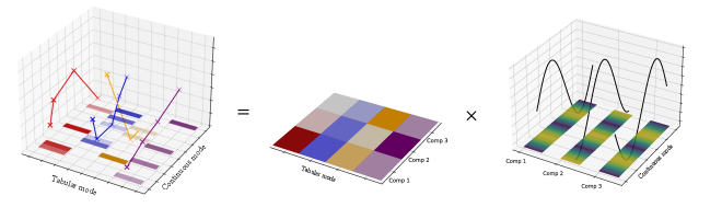
Figure 1: A pictorial illustration of FSVD: images on the horizontal ($x$-$y$) plane represent the FSVD of irregularly observed functional data, while the curves along the vertical ($z$) axis illustrate the smooth nature of functional data.

The third main contribution of this paper is the introduction of the concepts intrinsic basis functions and intrinsic basis vectors, which unify several crucial tasks of functional/longitudinal/time series data under the same framework of FSVD, as illustrated by Figure 2. These new concepts characterize intrinsic structures among functions with heterogeneous, and possibly dependent structures. Using the concept of intrinsic basis functions, we will show that FSVD is more general than FPCA (Ramsay and Silvermann, 2005; Yao et al., 2005a; Hsing and Eubank, 2015) and capable of effective dimension reduction and clustering. Meanwhile, the concept of intrinsic basis vectors allows FSVD to estimate factor models of time series under milder conditions than existing methods (Bai and Ng, 2002; Bai, 2003; Lam et al., 2011; Lam and Yao, 2012), making it suitable for estimating factor loadings and series from irregularly observed and non-stationary data. The above two frameworks offer two different interpretations of FSVD, adapted to the underlying structure of heterogeneous functional data. Additionally, the application of FSVD directly addresses the task of completion for functional data, which we refer to as functional completion in this paper.

Figure 2: An illustration of tasks associated with FSVD.

To demonstrate the utility of FSVD, we apply it to two real-world datasets. In a dataset that record the case counts of SARS-CoV-2 infection in 64 regions in 2020, FSVD was able to characterize heterogeneous trajectory patterns across regions that FPCA failed to identify. In a electronic health record dataset, FSVD performs data completion by leveraging a factor model across features, offering more reasonable completion results compared to existing methods.

1.1 Related Work

The framework of FSVD connects to a broad range of literature in functional data analysis, PCA, and SVD.

PCA and SVD versus Functional PCA and Functional SVD.

Principal Component Analysis (PCA) and Singular Value Decomposition (SVD) are related techniques essential for dimensionality reduction and feature extraction in matrix data. PCA is a statistical method that models data as samples of random vectors and performs dimensionality reduction based on the covariance matrix, whereas SVD is a linear algebra technique that factorizes any deterministic or random data matrix into low-rank components. While PCA relies on estimating the covariance matrix, it can be computed using SVD on the centralized data matrix, effectively bypassing explicit covariance computation—especially advantageous when the feature dimensionality exceeds the sample size. Beyond their interrelation, SVD has broader applications, such as spectral clustering (Ng et al., 2001), sparse PCA (Shen and Huang, 2008; Witten et al., 2009), canonical correlation analysis (Witten et al., 2009), and matrix completion (Candes and Plan, 2010; Candes and Recht, 2012), demonstrating its versatility.

A similar juxtaposition can be drawn between Functional PCA (FPCA) and Functional SVD (FSVD) as that between PCA and SVD for homogeneous functional data. FPCA typically involves estimating covariance functions, a complex task requiring substantial data and smoothness conditions on the covariance functions (Yao et al., 2005a; Hall et al., 2006; Hsing and Eubank, 2015; Descary and Panaretos, 2019; Zhang and Chen, 2022). In contrast, FSVD can perform dimension reduction directly on the data without estimating covariance functions, offering a more straightforward approach. In fact, the differences between FPCA and FSVD are more pronounced due to the complexity of functional data, which we will describe in the next paragraph.

Comparison with Existing Functional PCA- and SVD-type methods.

Most existing methods for the dimension reduction of functional data share a similar philosophy as PCA by adopting linear combinations of random components as low-dimensional representations of the data. They mostly fall under two frameworks: the first one focuses on the functional aspect and projects the data into deterministic basis functions, and the second one focuses on the tabular (e.g. feature or subject) aspect and projects the data into deterministic basis vectors.

Methods under the first framework project functions into deterministic eigenfunctions using Karhunen-Loève (KL) expansions and their extensions. For example, FPCA adopts the KL expansion for homogeneous functional data (Ramsay and Silvermann, 2005; Yao et al., 2005a; Yao and Lee, 2006; Hsing and Eubank, 2015); finite mixtures of KL expansions are used to account for clustering structures within heterogeneous functional data (Chiou and Li, 2007; Peng and Müller, 2008; Jacques and Preda, 2013); separable KL expansions handle separable covariance structures among dependent functional data (Lynch and Chen, 2018; Zapata et al., 2022; Liang et al., 2023; Tan et al., 2024); multivariate KL expansions are applied to project functional data into multivariate eigenfunctions (Chiou et al., 2014; Happ and Greven, 2018; Hu and Yao, 2022); and other extensions of KL expansions and FPCAs serve different purposes (Di et al., 2009; Chen and Lei, 2015; Panaretos and Tavakoli, 2013; Hörmann et al., 2015; Shou et al., 2015; Chen et al., 2017; Allen and Weylandt, 2019).

Methods under the second framework focusing on the tabular aspect include factor models for multivariate time series (Pan and Yao, 2008; Lam et al., 2011; Lam and Yao, 2012; Barigozzi et al., 2018; Zhang, Pan, Yao and Zhou, 2024; Zhang, Xue, Xu, Lee and Qu, 2024), which reduce the dimensionality of the subject/feature mode into deterministic factor loadings. Compared to these methods, FSVD offers a unified framework for handling heterogeneous functional data, being capable of providing dimensionality reduction for both functional and tabular aspects while adapting to their statistical structures. This allows FSVD to accomplish the tasks of both FPCA and factor models, making it applicable to a wider range of scenarios where different types of structures need to be captured and interpreted.

SVD-type methods have also appeared in the literature on functional data analysis (Huang et al., 2008, 2009; Yang et al., 2011; Zhang et al., 2013; Han et al., 2023). In these studies, Huang et al. (2008, 2009); Zhang et al. (2013); Han et al. (2023) implemented SVD-type methods to decompose a collection of functional data. Yang et al. (2011) applied singular value decomposition (SVD) to a compact operator induced by the cross-covariance between functional datasets, building upon the concept of “canonical expansion” of compact operators in functional analysis. In the approach of Huang et al. (2008), matrix SVD was extended to functional data by representing $\{X_{i}(t)\}_{i=1,\ldots,n;t\in\mathcal{T}}$ as a matrix with subjects/features and time as its two dimensions. This method assumed that all subjects/features were observed at the same time points and enforced continuity on the singular vectors associated with the time dimension. However, the assumption of identical time points is often impractical for many functional datasets. In contrast, the FSVD framework accommodates irregularly observed functional data and provides foundational theoretical guarantees that were previously unavailable.

Organization

The rest of this article is organized as follows. Section 2 introduces the theoretical framework of FSVD for fully observed functional data. In Section 3, we develop an estimation procedure of FSVD for noisy and irregularly observed functions, with its theoretical properties presented in Section 3.2. Section 4 connects FSVD to various tasks involving heterogeneous functional data, followed by extensive simulation studies in Section 5 to illustrate its effectiveness. We illustrate the usage of FSVD in two real-world applications in Section 6, and conclude with a discussion in Section 7. All proofs and additional real data analysis results are collected in the supplementary materials. The codes and datasets are publicly available at https://github.com/Jianbin-Tan/Functional-Singular-Value-Decompostion.

2 Foundations of Functional Singular Value Decomposition

Here we introduce the notation and preliminaries of this paper. Let $\mathcal{T}$ be a bounded closed interval in $\mathbb{R}$. Since we can rescale the functional domain, we assume $\mathcal{T}$ is $[0,1]$ throughout this article. Denote $\mathcal{L}^{2}(\mathcal{T})$ as the Hilbert space of square-integrable functions on $\mathcal{T}$, with the inner product $\langle\cdot,\cdot\rangle$ and norm $\|\cdot\|:=\sqrt{\langle\cdot,\cdot\rangle}$, where $\langle f,g\rangle=\int_{t\in\mathcal{T}}f(t)g(t)\ \mathrm{d}t$ for $f,g\in\mathcal{L}^{2}(\mathcal{T})$. For any vector $\bm{a}=(a_{1},\dots,a_{n})^{\top}$, we also denote $\|\bm{a}\|:=\sqrt{\sum_{i=1}^{n}a_{i}^{2}}$ as its $\ell_{2}$ norm. Define $\operatorname{span}(f_{1},\dots,f_{n})$ as the functional space spanned by $f_{1},\dots,f_{n}\in\mathcal{L}^{2}(\mathcal{T})$ and $\operatorname{dim}(f_{1},\dots,f_{n})$ as the dimension of $\operatorname{span}(f_{1},\dots,f_{n})$. Let $\mathbb{I}(\cdot)$ be the indicator function and $[Z]$ be the set of integers $\{1,\dots,Z\}$. For two sequences of non-negative real values $\{a_{n}\}$ and $\{b_{n}\}$, we say $a_{n}\lesssim b_{n}$ or $b_{n}\gtrsim a_{n}$ if there exists a constant $C>0$ such that $a_{n}\leq Cb_{n}$ for all $n$. Let $\operatorname{rank}(\cdot)$ denote the rank of a matrix.

Next, we introduce the notations in operator theory. Consider an operator $\mathcal{K}$ between two Hilbert spaces $\mathcal{H}_{1}$ and $\mathcal{H}_{2}$, each with inner product $\langle\cdot,\cdot\rangle_{i}$ and norms $\|\cdot\|_{i}$ for $i=1,2$. Define $\operatorname{Dom}(\mathcal{K})$ as the domain of $\mathcal{K}$, and denote $\operatorname{Im}(\mathcal{K}):=\{\mathcal{K}x;x\in\operatorname{Dom}(\mathcal{K})\}$ and $\operatorname{Null}(\mathcal{K}):=\{x\in\operatorname{Dom}(\mathcal{K});\mathcal{K}x=\bm{0}\}$ as the image and null spaces of $\mathcal{K}$, where $\bm{0}$ is the zero element in $\mathcal{H}_{2}$. Define the composition of two operators $\mathcal{K}_{1}$ and $\mathcal{K}_{2}$ as $\mathcal{K}_{1}\mathcal{K}_{2}$ whenever $\operatorname{Im}(\mathcal{K}_{2})\subset\operatorname{Dom}(\mathcal{K}_{1})$. Given an operator $\mathcal{K}$ from $\mathcal{H}_{1}$ to $\mathcal{H}_{1}$, if there exist $e\in\mathcal{H}_{1}$ and $\lambda\in\mathbb{R}$ such that $\mathcal{K}e=\lambda e$, $\lambda$ and $e$ are called the eigenvalue and eigenfunction of $\mathcal{K}$, respectively. An operator $\mathcal{K}$ is compact if for any bounded sequence $\{x_{N};N\geq 1\}$ in $\mathcal{H}_{1}$, $\{\mathcal{K}x_{N};N\geq 1\}$ has a convergent subsequence in $\mathcal{H}_{2}$.

In the following Theorem 1, we describe the functional singular value decomposition (FSVD) for deterministic functions $X_{1},\ldots,X_{n}\in\mathcal{H}$, where $\mathcal{H}\subseteq\mathcal{L}^{2}(\mathcal{T})$ is a Hilbert space.

Theorem 1 (Existence and Basic Properties of Functional Singular Value Decomposition).

Suppose $X_{1},\ldots,X_{n}\in\mathcal{H}$. Then there exists an FSVD of $X_{1},\ldots,X_{n}$:

$$\left[\begin{array}[]{c}X_{1}\\ \vdots\\ X_{n}\end{array}\right]=\sum_{r=1}^{R}\rho_{r}\bm{a}_{r}\phi_{r},$$ (2)

where $\rho_{1}\geq\dots\geq\rho_{R}>0$ are singular values, $\bm{a}_{1},\dots,\bm{a}_{R}\in\mathbb{R}^{n}$ are singular vectors, $\phi_{1},\dots,\phi_{R}\in\mathcal{H}$ are singular functions, and $R\leq n$ is the rank. Here, $\bm{a}_{1},\dots,\bm{a}_{R}$ and $\phi_{1},\dots,\phi_{R}$ are orthonormal in the sense that $\bm{a}_{r}^{\top}\bm{a}_{r^{\prime}}=\langle\phi_{r},\phi_{r^{\prime}}\rangle=\mathbb{I}(r=r^{\prime})$ for $r,r^{\prime}\in[R]$.

Define $\mathcal{X}_{n}:\mathcal{H}\to\mathbb{R}^{n}$,

$$\mathcal{X}_{n}:f\mapsto\big{(}\langle X_{1},f\rangle,\dots,\langle X_{n},f\rangle\big{)}^{\top},\ \forall f\in\mathcal{H},$$ (3)

and $\mathcal{X}_{n}^{\ast}$ denotes the adjoint operator of $\mathcal{X}_{n}$. Then $\mathcal{X}_{n}$ is a compact operator; $\rho_{r}^{2}$s are the non-zero eigenvalues of both the self-adjoint operators $\mathcal{X}_{n}^{*}\mathcal{X}_{n}:\mathcal{H}\to\mathcal{H}$ and $\mathcal{X}_{n}\mathcal{X}_{n}^{*}:\mathbb{R}^{n}\to\mathbb{R}^{n}$; $\phi_{r}$ is an eigenfunction of $\mathcal{X}_{n}^{*}\mathcal{X}_{n}$ and $\bm{a}_{r}$ is an eigenvector of $\mathcal{X}_{n}\mathcal{X}_{n}^{*}$, corresponding to the eigenvalue $\rho_{r}^{2}$.

Theorem 1 demonstrates that functional data can be viewed as the compact operator $\mathcal{X}_{n}$ between $\mathcal{H}$ and $\mathbb{R}^{n}$, similar to matrix data being viewed as a linear transformation. The compactness of $\mathcal{X}_{n}$ then leads to the FSVD of $X_{i}$s in Theorem 1.

The following theorem characterizes the uniqueness of FSVD.

Theorem 2 (Uniqueness of FSVD).

If there exist two FSVDs of $X_{1},\ldots,X_{n}$: $\big{\{}\rho_{r},\bm{a}_{r},\phi_{r};r=1,\dots,R\big{\}}$, $\big{\{}\tilde{\rho}_{r},\tilde{\bm{a}}_{r},\tilde{\phi}_{r};r=1,\dots,\tilde{R}\big{\}}$ such that $\rho_{1}\geq\cdots\geq\rho_{R}>0$, $\tilde{\rho}_{1}\geq\cdots\geq\tilde{\rho}_{\tilde{R}}>0$, $\bm{a}_{r}^{\top}\bm{a}_{r^{\prime}}=\langle\phi_{r},\phi_{r^{\prime}}\rangle=\tilde{\bm{a}}_{r}^{\top}\tilde{\bm{a}}_{r^{\prime}}=\langle\tilde{\phi}_{r},\tilde{\phi}_{r^{\prime}}\rangle=\mathbb{I}(r=r^{\prime})$, and satisfying $\sum_{r=1}^{R}\rho_{r}\bm{a}_{r}\phi_{r}=\sum_{r=1}^{\tilde{R}}\tilde{\rho}_{r}\tilde{\bm{a}}_{r}\tilde{\phi}_{r}$, then $R=\tilde{R}$ and $\rho_{r}=\tilde{\rho}_{r}$ for all $r\in[R]$.

Furthermore, if $\rho_{1}>\cdots>\rho_{R}>0$ are distinct, then $(\tilde{\bm{a}}_{r},\tilde{\phi}_{r})=\pm(\bm{a}_{r},\phi_{r})$.

If there exists a block of identical singular values, say $\rho_{r_{1}-1}>\rho_{r_{1}}=\cdots=\rho_{r_{2}}>\rho_{r_{2}+1}$, then there exists an orthogonal matrix $\bm{B}\in\mathbb{R}^{(r_{2}-r_{1}+1)\times(r_{2}-r_{1}+1)}$ such that $(\tilde{\bm{a}}_{r_{1}},\dots,\tilde{\bm{a}}_{r_{2}})=({\bm{a}}_{r_{1}},\dots,{\bm{a}}_{r_{2}})\bm{B}$ and $(\tilde{\phi}_{r_{1}},\dots,\tilde{\phi}_{r_{2}})=({\phi}_{r_{1}},\dots,{\phi}_{r_{2}})\bm{B}$.

Theorem 2 shows that when the singular values are distinct, the singular functions and singular vectors are unique up to sign-flipping; when there are multiple identical singular values, the corresponding subspaces spanned by the singular vectors or singular functions are uniquely identifiable.

Theorem 3 (Sequential Formation of FSVD).

Define the following sequences for $r=1,2,\dots,R$:

$$\begin{split}(g_{1r},\dots,g_{nr})=&\operatorname*{arg\,min}_{f_{1},\dots,f_{n}\in\mathcal{H}}\sum_{i=1}^{n}\bigg{\|}X_{i}-\sum_{l=1}^{r-1}g_{il}-f_{i}\bigg{\|}^{2}\\ \text{\leavevmode\nobreak\ \leavevmode\nobreak\ subject to\leavevmode\nobreak\ \leavevmode\nobreak\ }&\operatorname{dim}(f_{1},\dots,f_{n})=1.\end{split}$$

Represent $g_{ir}=b_{ir}\phi_{r}^{0}$ with $\|\phi_{r}^{0}\|=1$, and define $\rho_{r}^{0}:=\sqrt{\sum_{i=1}^{n}b_{ir}^{2}}$ and $\bm{a}_{r}^{0}:=(b_{1r},\dots,b_{nr})^{\top}/\rho_{r}^{0}$. Then $\{\rho_{r}^{0},\bm{a}_{r}^{0},\phi_{r}^{0}\}_{r\in[R]}$ forms the FSVD of $X_{1},\dots,X_{n}$.

Theorem 3 shows that the $r$th singular component is the optimal rank-one approximation for the functions $X_{1},\ldots,X_{n}$ after subtraction of the first $(r-1)$ singular components.

3 FSVD for Irregularly Observed Functional Data

In real-world applications, functional curves are typically observed with noise at discrete time points, rather than being directly measured across the entire continuum. To accommodate such practical scenarios, we extend the aforementioned framework of FSVD to discretely observed functional data. We specifically focus on the following model that is widely considered in the literature (Yao et al., 2005a; Cai and Yuan, 2011; Hsing and Eubank, 2015; Wang et al., 2016; Nie et al., 2022):

$$Y_{ij}=X_{i}(T_{ij})+\varepsilon_{ij},\quad j\in[J_{i}],\ i\in[n],$$ (4)

where $\big{\{}T_{ij};j\in[J_{i}]\big{\}}$ is the collection of observable time points for trajectory $X_{i}$, $\big{\{}\varepsilon_{ij};j\in[J_{i}]\big{\}}$ are the mean-zero noise variables, and $\big{\{}Y_{ij};j\in[J_{i}]\big{\}}$ are the noisy discrete observations of $X_{i}$ for each $i$. In this model, we allow the observation time points to be irregular, i.e., $\big{\{}T_{ij};j\in[J_{i}]\big{\}}$ may vary across different $i$. Under this setting, we cannot directly evaluate their FSVD via the approach developed in Section 2 since $X_{i}$ are incompletely observed with added noise.

To obtain FSVD under model (4), we assume $X_{i}$ are contained in a reproducing kernel Hilbert space $\mathcal{H}(\mathbb{K})\subset\mathcal{L}^{2}(\mathcal{T})$ that satisfies certain smoothness conditions. Before getting into the details, we first introduce some notation and preliminaries in the context of RKHS. Let $\mathcal{H}$ be a Hilbert space of functions on $\mathcal{T}$ with inner product $\langle\cdot,\cdot\rangle_{\mathcal{H}}$ and norm $\|\cdot\|_{\mathcal{H}}$. The functional space $\mathcal{H}$ is called an RKHS if there exists a kernel $\mathbb{K}$ on $\mathcal{T}\times\mathcal{T}$ such that

$$\mathbb{K}(t,\cdot)\in\mathcal{H}\ \text{and}\ f(t)=\langle f,\mathbb{K}(t,\cdot)\rangle_{\mathcal{H}}$$

for all $t\in\mathcal{T}$ and $f\in\mathcal{H}$. We denote $\mathcal{H}$ as $\mathcal{H}(\mathbb{K})$ because it can be shown that $\mathbb{K}$, the reproducing kernel of $\mathcal{H}$, is unique to $\mathcal{H}$. For a more detailed exposition of RKHS theory, see Aronszajn (1950).

To avoid overfitting and encourage smoothness in the estimates of $X_{i}$ in $\mathcal{H}(\mathbb{K})$, we will use the penalization term $\|\mathcal{P}(\cdot)\|_{\mathcal{H}}$, where $\mathcal{P}$ is a projection operator from $\mathcal{H}(\mathbb{K})$ onto its subspace. This framework is commonly adopted in the literature on RKHS regression (Schölkopf et al., 2001; Yuan and Cai, 2010; Gu, 2013; Hsing and Eubank, 2015).

In this article, we focus on $\mathcal{H}(\mathbb{K})$ being a subset of $\mathcal{L}^{2}(\mathcal{T})$. This can be achieved if there exists a constant $C_{\mathbb{K}}$ such that $\sup_{t\in\mathcal{T}}\sqrt{\mathbb{K}(t,t)}\leq C_{\mathbb{K}}$:

$$\|f\|\leq\sup_{t\in\mathcal{T}}|f(t)|=\sup_{t\in\mathcal{T}}|\langle f,\mathbb{K}(\cdot,t)\rangle_{\mathcal{H}}|\leq\|f\|_{\mathcal{H}}\cdot\sup_{t\in\mathcal{T}}\sqrt{\mathbb{K}(t,t)}\leq C_{\mathbb{K}}\|f\|_{\mathcal{H}},\forall f\in\mathcal{H}(\mathbb{K}),$$

which in turn leads to $\mathcal{H}(\mathbb{K})\subset\mathcal{L}^{2}(\mathcal{T})$. One common choice of an RKHS contained in $\mathcal{L}^{2}(\mathcal{T})$ to reflect the smoothness of functional data is the Sobolev space (Yuan and Cai, 2010; Hsing and Eubank, 2015):

$$\mathcal{W}^{2}_{q}(\mathcal{T}):=\big{\{}f:\mathcal{T}\rightarrow\mathbb{R};\ D^{0}f,\cdots,D^{q-1}f\ \text{are continuous and }D^{q}f\in\mathcal{L}^{2}(\mathcal{T})\big{\}}\subseteq\mathcal{L}^{2}(\mathcal{T}),$$

where $D^{q}$ is the order-$q$ differential operator. Under this setting, it is common to take $\mathcal{P}$ to be the projection operator from $\mathcal{W}^{2}_{q}(\mathcal{T})$ onto $\mathcal{H}_{1}:=\big{\{}h(t)=\int_{0}^{t}g(s)(t-s)^{q-1}\ \mathrm{d}s/(q-1)!;g\in\mathcal{L}^{2}(\mathcal{T})\big{\}}\subset\mathcal{W}^{2}_{q}(\mathcal{T})$ (Gu, 2013; Hsing and Eubank, 2015). Therefore, $\|\mathcal{P}X_{i}\|_{\mathcal{H}}$ becomes $\|D^{q}X_{i}\|$, measuring the smoothness of $X_{i}$ in terms of its $q$th derivative.

3.1 Joint Kernel Ridge Regression for FSVD

With the assumption of $X_{1},\ldots,X_{n}$ contained in an RKHS $\mathcal{H}(\mathbb{K})\subset\mathcal{L}^{2}(\mathcal{T})$, we ensure the singular components of $X_{i}$s are contained in $\mathcal{H}(\mathbb{K})$ as per Theorem 1. Based on Theorem 3, we propose to estimate the first singular component by computing

$$\begin{split}&\operatorname*{arg\,min}_{f_{1},\dots,f_{n}\in\mathcal{H}(\mathbb{K})}\sum_{i=1}^{n}\left(\frac{1}{J_{i}}\sum_{j=1}^{J_{i}}\big{\{}Y_{ij}-f_{i}(T_{ij})\big{\}}^{2}+\nu\left\|\mathcal{P}f_{i}\right\|^{2}_{\mathcal{H}}\right)\\ &\text{\leavevmode\nobreak\ \leavevmode\nobreak\ subject to\leavevmode\nobreak\ \leavevmode\nobreak\ }\text{dim}(f_{1},\ldots,f_{n})=1.\end{split}$$ (5)

Here, $\mathcal{P}$ is a projection operator discussed earlier and $\nu$ is a tuning parameter. We set that $f_{i}=a_{i1}\phi_{1}$ and $\bm{a}_{1}=(a_{11},\dots,a_{n1})^{\top}$; then (5) is equivalent to

$$\operatorname*{arg\,min}_{\bm{a}_{1}\in\mathbb{R}^{n},\phi_{1}\in\mathcal{H}(\mathbb{K})}\sum_{i=1}^{n}\frac{1}{J_{i}}\sum_{j=1}^{J_{i}}\big{\{}Y_{ij}-a_{i1}\phi_{1}(T_{ij})\big{\}}^{2}+\nu\|\bm{a}_{1}\|^{2}\cdot\|\mathcal{P}\phi_{1}\|_{\mathcal{H}}^{2}.$$ (6)

Remark 1 (Connections to existing functional data/kernel ridge regression/SVD methods).

The optimizations (5) and (6) are related to many existing methods in the literature of functional data/kernel ridge regression/SVD methods. First, note that when $f_{i}$s are free of $i$, the optimization (5) reduces to the estimation of a mean function for independent and identically distributed (i.i.d.) functional data $X_{i}$s (Cai and Yuan, 2011; Hsing and Eubank, 2015). In this context, (5) relaxes the i.i.d. assumption to allow for varying mean functions for $X_{i}$s. Moreover, (5) can also be a standard kernel ridge regression (Schölkopf et al., 2001; Gu, 2013) when $n=1$. When $n>1$, the rank-one constraint we impose to link the estimations of $X_{i}$s together allows for the borrowing of information across functions in the implementation of a joint kernel ridge regression on $Y_{ij}$s. Finally, being equivalent to (5), (6) can be viewed as one type of penalized decomposition on the observed data $Y_{ij}$s, similar to existing SVD-type methods for matrices (Shen and Huang, 2008; Witten et al., 2009; Yu et al., 2016) or functional data (Huang et al., 2008, 2009; Zhang et al., 2013).

It is worth noting that the regularization of $X_{i}$s in (5) is transferred to $\phi_{1}$ and $\bm{a}_{1}$ in (6). The minimization over the function $\phi_{1}$ can then be reformulated into a finite-dimensional optimization problem as demonstrated by the following theorem.

Theorem 4.

Assume $\operatorname{dim}(\operatorname{Null}(\mathcal{P}))<\infty$. Let $h_{1},\cdots,h_{q}$ be a collection of basis functions of $\operatorname{Null}(\mathcal{P})$ and define $g_{ij}:=\mathcal{P}\big{\{}\mathbb{K}(\cdot,T_{ij})\big{\}}$. Then there exist $u_{m}\in\mathbb{R}$, $m\in[q]$, and $w_{ij}\in\mathbb{R}$, $i\in[n]$ and $j\in[J_{i}]$, such that the minimizer of $\phi_{1}$ in (6) is represented as $\sum_{m=1}^{q}{u}_{m}h_{m}+\sum_{i=1}^{n}\sum_{j=1}^{J_{i}}{w}_{ij}g_{ij}$. As a result, (6) can be reformulated as

$$\begin{split}\min_{\bm{a}_{1}\in\mathbb{R}^{n},\bm{u}\in\mathbb{R}^{q},\bm{w}\in\mathbb{R}^{J}}&\sum_{i=1}^{n}\frac{1}{J_{i}}\sum_{j=1}^{J_{i}}\bigg{[}Y_{ij}-a_{i1}\bigg{\{}\sum_{m=1}^{q}u_{m}h_{m}(T_{ij})+\sum_{i_{1}=1}^{n}\sum_{j_{1}=1}^{J_{i}}w_{i_{1}j_{1}}g_{i_{1}j_{1}}(T_{ij})\bigg{\}}\bigg{]}^{2}\\ &+\nu\|\bm{a}_{1}\|^{2}\cdot\bm{w}^{\top}\bm{G}\bm{w},\end{split}$$ (7)

where $\bm{u}=(u_{1},\cdots,u_{q})^{\top}$, $\bm{w}=\big{(}w_{ij};i\in[n],j\in[J_{i}]\big{)}^{\top}\in\mathbb{R}^{J}$ with $J=\sum_{i=1}^{n}J_{i}$ being the total number of observations, and the entries of the matrix $\bm{G}$ are $\langle g_{i^{\prime}j^{\prime}},g_{i^{\prime\prime}j^{\prime\prime}}\rangle_{\mathcal{H}}$ for all $i^{\prime},i^{\prime\prime}\in[n],j^{\prime}\in[J_{i^{\prime}}],j^{\prime\prime}\in[J_{i^{\prime\prime}}]$.

Theorem 4 can be seen as an extension of the Representer Theorem for kernel ridge regression (Schölkopf et al., 2001) to our rank-one-constrained kernel ridge regression (5). This theorem paves the way to compute FSVD on infinite-dimensional functions through finite dimensional optimization.

When $\mathcal{H}(\mathbb{K})$ is taken as $\mathcal{W}^{2}_{q}(\mathcal{T})$ with $\|\mathcal{P}\phi_{1}\|_{\mathcal{H}}=\|D^{q}\phi_{1}\|$ as mentioned previously, we have a simpler representer theorem for the optimization (6). In detail, suppose that $J_{i}>q$, $i\in[n]$. Then there exist $w_{ij}\in\mathbb{R}$, $i\in[n]$ and $j\in[J_{i}]$, such that the minimizer of $\phi_{1}$ in (6) can be represented as $\phi_{1}(t)=\sum_{i=1}^{n}\sum_{j=1}^{J_{i}}{w}_{ij}N_{ij}(t)$, and (6) can be transformed into

$$\min_{\bm{a}_{1}\in\mathbb{R}^{n},\bm{w}\in\mathbb{R}^{J}}\sum_{i=1}^{n}\frac{1}{J_{i}}\sum_{j=1}^{J_{i}}\bigg{\{}Y_{ij}-a_{i1}\sum_{i_{1}=1}^{n}\sum_{j_{1}=1}^{J_{i}}w_{i_{1}j_{1}}N_{i_{1}j_{1}}(T_{ij})\bigg{\}}^{2}+\nu\|\bm{a}_{1}\|^{2}\cdot\bm{w}^{\top}\bm{H}\bm{w},$$ (8)

where $\bm{w}=\big{(}w_{ij};i\in[n],j\in[J_{i}]\big{)}^{\top}\in\mathbb{R}^{J}$, $\big{\{}N_{ij};i\in[n],j\in[J_{i}]\big{\}}$ are the natural spline basis functions of order $2q$ with knots $\big{\{}T_{ij};i\in[n],j\in[J_{i}]\big{\}}$, and the matrix $\bm{H}$ has entries $\langle D^{q}N_{i^{\prime}j^{\prime}},D^{q}N_{i^{\prime\prime}j^{\prime\prime}}\rangle$ for all $i^{\prime},i^{\prime\prime}\in[n]$, $j^{\prime}\in[J_{i^{\prime}}]$, $j^{\prime\prime}\in[J_{i^{\prime\prime}}]$. See Part B.1 in the Supplementary Materials for the demonstration.

We employ an alternating minimization to obtain the minimizers of $\bm{a}_{1}$ and $\bm{w}$ from (8). Note that $\bm{a}_{1}$ and $\bm{w}$ are identifiable only up to a scalar multiplication, we always scale $\bm{a}_{1}$ such that $\|\bm{a}_{1}\|=1$ in solving the alternating minimization. The procedure of alternating minimization is summarized in Algorithm 1, where the initialization and tuning selection procedures are detailed in Part B.2 of the Supplementary Materials and the subsequent remark, respectively.

Algorithm 1 Alternating Minimization for Estimating the First Component

1:Input $\hat{\bm{a}}_{1}^{(0)}$, $\big{\{}Y_{ij};j\in[J_{i}],i\in[n]\big{\}}$, tuning parameter $\nu$, threshold value $\tau$, and maximum iteration number $H$.

2:$h=0$ and $\hat{\bm{a}}^{(0)}=\hat{\bm{a}}_{1}^{(0)}$.

3:Repeat

4: For $i=1,\dots,n$ do

5:  Solve

$$\hat{\bm{w}}=\min_{\bm{w}\in\mathbb{R}^{J}}\sum_{i=1}^{n}\frac{1}{J_{i}}\sum_{j=1}^{J_{i}}(\hat{a}_{i}^{(h)})^{2}\bigg{\{}Y_{ij}/a_{i1}^{(h)}-\sum_{i_{1}=1}^{n}\sum_{j_{1}=1}^{J_{i}}w_{i_{1}j_{1}}N_{ij}(T_{ij})\bigg{\}}^{2}+\nu\bm{w}^{\top}\bm{N}\bm{w}.$$ (9)

6:  $\widehat{\rho\phi}^{(h)}(T_{ij})=\sum_{i_{1}=1}^{n}\sum_{j_{1}=1}^{J_{i}}\hat{w}_{i_{1}j_{1}}N_{i_{1}j_{1}}(T_{ij})$ for $i\in[n]$ and $j\in[J_{i}]$.

7:  Let

$$\tilde{a}_{i}^{(h+1)}=\frac{\frac{1}{J_{i}}\sum_{j=1}^{J_{i}}Y_{ij}\widehat{\rho\phi}^{(h)}(T_{ij})}{\frac{1}{J_{i}}\sum_{j=1}^{J_{i}}\big{\{}\widehat{\rho\phi}^{(h)}(T_{ij})\big{\}}^{2}+\nu\hat{\bm{w}}^{\top}\bm{N}\hat{\bm{w}}}.$$ (10)

8:  Update $\hat{\bm{a}}^{(h+1)}:=\left(\tilde{a}_{1}^{(h+1)},\cdots,\tilde{a}^{(h+1)}_{n}\right)^{\top}/\sqrt{\left(\tilde{a}_{1}^{(h+1)}\right)^{2}+\cdots+\left(\tilde{a}^{(h+1)}_{n}\right)^{2}}$.

9: End for

10: $h=h+1$.

11:Until $h\geq H$ or $\|\widehat{\rho\phi}^{(h-1)}-\widehat{\rho\phi}^{(h)}\|/\|\widehat{\rho\phi}^{(h-1)}\|\leq\tau$.

12:Set $\hat{\bm{a}}_{1}$, $\hat{\phi}_{1}$, and $\hat{\rho}_{1}$ as $\hat{\bm{a}}^{(h)}$, $\widehat{\rho\phi}^{(h)}/\|\widehat{\rho\phi}^{(h)}\|$, and $\|\widehat{\rho\phi}^{(h)}\|$, respectively.

13:Output $\hat{\bm{a}}_{1}$, $\hat{\phi}_{1}$, and $\hat{\rho}_{1}$.

It can be shown that Algorithm 1 reduces to the power iteration method on matrices when the observed time grids are aligned across different functions; see Part B.1 in the Supplementary Materials for the discussion. For the irregular case, Algorithm 1 incorporates non-parametric smoothing via (9) during iterations, leading to an iteratively reweighted smoothing spline procedure for the data $Y_{ij}$s. This procedure is similar to estimating a smooth mean function from $Y_{ij}$s when $X_{i}$s are i.i.d. functional data (Cai and Yuan, 2011; Hsing and Eubank, 2015). When this homogeneous condition is not met, estimating mean functions is generally invalid and inconsistent. Nonetheless, we can still perform FSVD via Algorithm 1, iteratively smoothing the functional data to estimate their singular functions.

Based on Theorem 3, we propose to sequentially estimate the $r$th singular component for $r=1,\ldots,R$ using Algorithm 1. In each iteration, we replace the data $Y_{ij}$ by $Y_{ij}^{(r)}$, defined as

$$Y_{ij}-\sum_{l=1}^{r-1}\hat{\rho}_{l}\hat{{a}}_{i{l}}\hat{\phi}_{l}(T_{ij}),\ j\in[J_{i}],i\in[n],$$

where $\{\hat{\rho}_{l}\hat{{a}}_{i{l}}\hat{\phi}_{l};l\in[r-1]\}$ are the first $(r-1)$ estimated singular component via Algorithm 1. This procedure is summarized in Algorithm 2.

Algorithm 2 General Procedure of FSVD

1:Input observed data $\big{\{}Y_{ij};j\in[J_{i}],i\in[n]\big{\}}$ and $R>1$.

2:Input $\hat{\bm{a}}_{1}^{(0)}$, tuning parameter $\nu$, threshold value $\tau$, and maximum iteration number $H$.

3:Output $\hat{\bm{a}}_{1}$, $\hat{\phi}_{1}$, and $\hat{\rho}_{1}$ from Algorithm 1.

4:For $r=2,\dots,R$ do

5: Input $\hat{\bm{a}}_{r}^{(0)}$, tuning parameter $\nu_{r}$.

6: Calculate

$${Y}_{ij}^{(r)}=Y_{ij}-\sum_{l=1}^{r-1}\hat{\rho}_{l}\hat{{a}}_{i{l}}\hat{\phi}_{l}(T_{ij}),\ j\in[J_{i}],i\in[n].$$

7: Implement Algorithm 1 with $\hat{\bm{a}}_{r}^{(0)}$, $\big{\{}{Y}^{(r)}_{ij};j\in[J_{i}],i\in[n]\big{\}}$, $\nu_{r}$, $\tau$, and $H$.

8: Output $\hat{\bm{a}}_{r}$, $\hat{\phi}_{r}$, $\hat{\rho}_{r}$.

9:End for

Hyperparameter Selection for $\nu$ and $R$.

We propose a cross-validation (CV) criterion based on Algorithm 1 to select the tuning parameter $\nu$ for each FSVD component. For each $i$, we first divide the data $\{T_{ij},Y_{ij};j\in[J_{i}]\}$ into five groups, i.e., $\{T_{ij},Y_{ij};j\in[J_{i}]\}=\cup_{m=1}^{5}\{T_{ij,m},Y_{ij,m};j\in[J_{i,m}]\},\ \forall i\in[n].$ For given $i$ and $m$, $\{T_{ij,m},Y_{ij,m};j\in[J_{i,m}]\}$ is a proper subset of $\{T_{ij},Y_{ij};j\in[J_{i}]\}$. Denote by $\hat{\rho}_{1}^{(-m)}$, $\hat{\phi}_{1}^{(-m)}$, and $\hat{\bm{a}}_{1}^{(-m)}$ the outputs of Algorithm 1 with the input data excluding the $m$th group. Given this, define

$$\operatorname{CV}(\nu)=\frac{1}{5}\sum_{m=1}^{5}\sum_{i=1}^{n}\frac{1}{J_{i}}\sum_{j=1}^{J_{i,m}}\bigg{\{}Y_{ij,m}-\hat{\rho}_{1}^{-(m)}\hat{a}_{i1}^{(-m)}\hat{\phi}_{1}^{(-m)}(T_{ij,m})\bigg{\}}^{2},$$

where $Y_{ij,m}-\hat{\rho}_{1}^{-(m)}\hat{a}_{i1}^{(-m)}\hat{\phi}_{1}^{(-m)}(T_{ij})$, $j\in[J_{i,m}]$, are set to 0 if $\{T_{ij,m},Y_{ij,m};j\in[J_{i,m}]\}$ is an empty set. We select $\nu$ for the first singular component by minimizing $\operatorname{CV}(\nu)$. Note that the optimal value of $\nu$ may vary across different singular components (see Theorem 5). Therefore, when evaluating the $r$th FSVD component, we select $\nu$ by applying the above CV criterion based on $\{Y_{ij}^{(r)};i\in[n],j\in[J_{i}]\}$.

To determine the rank $R$, we can select $R$ by the ratio of singular values: $\operatorname*{arg\,max}_{r\leq R_{max}}\frac{\hat{\rho}_{r}}{\hat{\rho}_{r+1}}$, where $R_{max}$ is a predetermined upper bound for $R$. We can also select $R$ based on additional assumptions on the measurement errors $\varepsilon_{ij}$s. Specifically, if $\{\varepsilon_{ij};j\in[J_{i}]\}$ follow a mean-zero Gaussian distribution with variance $\sigma_{i}^{2}$ for each $i$. We can adopt the Akaike information criterion (AIC) to select the $R$ by minimizing

$$\text{AIC}(R):=\sum_{i=1}^{n}J_{i}\log(\hat{\sigma}^{2}_{i,R})+2nR,$$ (11)

where $\hat{\sigma}^{2}_{i,R}=\frac{1}{J_{i}}\sum_{j=1}^{J_{i}}\big{\{}Y_{ij}-\sum_{k=1}^{R}\hat{\rho}_{r}\hat{{a}}_{i{r}}\hat{\phi}_{r}(T_{ij})\big{\}}^{2}$. The AIC is constructed by viewing our procedure as a linear regression of $Y_{ij}$ against the covariates $(\hat{\phi}_{1}(T_{ij}),\dots,\hat{\phi}_{K}(T_{ij}))$ for $i\in[n]$ and $j\in[J_{i}]$, similar to that in Li et al. (2013). Alternative selection criteria can be established based on the connection of FSVD with factor models, as detailed in Section 4.3. In such scenarios, $R$ can be selected based on information criteria for factor models (Bai and Ng, 2002; Li et al., 2013).

3.2 Statistical Theory

Next, we establish statistical guarantees for FSVD with irregularly observed functional data. We assume that $\{X_{i};i\in[n]\}$ are deterministic functions from $\mathcal{W}_{q}^{2}(\mathcal{T})$ with $q>1/2$, and the true singular values, singular functions, and singular vectors of $X_{i}$s are denoted as $\rho_{r}^{0}$, $\phi_{r}^{0}$, and $\bm{a}_{r}^{0}$ for $r\in[R]$, respectively. By Algorithm 1, the estimates of $\rho_{r}^{0}\phi_{r}^{0}$ and $\bm{a}_{r}^{0}$ at the $h$th step for the $r$th singular component are denoted as $\widehat{\rho\phi}_{r}^{(h)}$ and $\hat{\bm{a}}_{r}^{(h)}$ for $r\in[R]$, while their final outputs are denoted as $\hat{\rho}_{r}\hat{\phi}_{r}$ and $\hat{\bm{a}}_{r}$, $r\in[R]$. We define the sine values of the pairs of vectors/functions to measure the estimation errors:

$$\begin{split}\operatorname{dist}(\bm{u},\bm{v})&=\sqrt{1-\bigg{(}\frac{\bm{u}^{\top}\bm{v}}{\|\bm{u}\|\cdot\|\bm{v}\|}\bigg{)}^{2}},\quad\forall\bm{u},\bm{v}\in\mathbb{R}^{n};\\ \operatorname{dist}(f,g)&=\sqrt{1-\bigg{(}\frac{\langle f,g\rangle}{\|f\|\cdot\|g\|}\bigg{)}^{2}},\quad\forall f,g\in\mathcal{L}^{2}(\mathcal{T}).\end{split}$$ (12)

In the following, we only state the theoretical result for estimating the first singular component, while the results for other components can be similarly obtained. We introduce the following assumptions.

Assumption 1.

The numbers of observed time points $\big{\{}J_{i};i\in[n]\big{\}}$ are fixed positive integers, and there exists a number $m$ and a constant $C$ such that $\min_{i\in[n]}J_{i}\geq Cm$. In addition, the time points $\{T_{ij};j\in[J_{i}]\}$ are independently drawn from a uniform distribution on $[0,1]$ for each $i$.

Assumption 2.

The measurement errors $\varepsilon_{ij}$ are independent of $T_{ij}$ and follow mean-zero sub-Gaussian distributions that satisfy $\mathbb{E}\exp({\lambda\varepsilon_{ij}})\leq\exp(\lambda^{2}\sigma^{2}/2)$ for all $i$, $j$, and $\lambda\in\mathbb{R}$.

In Assumption 2, $\sigma$ measures the uncertainty level of $\varepsilon_{ij}$s. For example, $\sigma^{2}$ can be an upper bound of the variance of $\varepsilon_{ij}$ if the measurement noises follow Gaussian distributions.

Assumption 3.

$\big{\|}D^{q}\left(\sum_{i=1}^{n}a_{i}X_{i}\right)\big{\|}\lesssim\rho_{R}^{0}$ for all $\{a_{i};i\in[n]\}$ satisfying $\sum_{i=1}^{n}a_{i}^{2}\leq 1$.

Assumption 3 ensures that the $\mathcal{L}^{2}$ norm of singular functions’ $q$th derivatives, i.e., $\|D^{q}\phi_{r}^{0}\|^{2}$ $=\big{\|}D^{q}\left(\sum_{i=1}^{n}a_{ir}^{0}X_{i}\right)\big{\|}^{2}/(\rho_{r}^{0})^{2}$, $r\in[R]$, is bounded by a constant. This helps control the bias of the estimated singular functions via optimization (8). Similar conditions have been adopted in the theoretical analysis of methods using smoothing splines (Speckman, 1985; Cai and Yuan, 2011; Hsing and Eubank, 2015).

Assumption 4.

The ratio of singular values $\kappa=\rho_{1}^{0}/\rho_{2}^{0}$, $m$, and the signal-to-noise ratio $\rho_{1}^{0}/\sigma$ satisfy $\kappa\gtrsim R$, $m^{{1}/{(2q+1)}}\gtrsim\log(n)$, $m^{q-1}\gtrsim(\rho_{1}^{0})^{2}$, and $\rho_{1}^{0}/\sigma\gtrsim n^{1/2+1/(2q-1)}/\sqrt{m}$.

Assumption 4 suggests that the ratio of singular values is sufficiently large, the observed time grids of functions are sufficiently dense, and the signal-to-noise ratio is adequately high. These conditions can be achieved if $R$ grows with $\kappa$ and $n$ and $\rho_{1}^{0}$ grow with $m$, ensuring that errors arising from noises and discrete observation are controllable during iteration updates.

Theorem 5 (Error Bound of FSVD with Irregularly Observed Data).

Suppose Assumptions 1 – 4 hold. We assume that the tuning parameter $\nu$ satisfies $m^{-q/(2q+1)}+\frac{\sigma}{\rho_{1}^{0}}\cdot\sqrt{\frac{n}{m}}\cdot x\lesssim\nu^{1/(2q)}$ and $\frac{\sigma}{\rho_{1}^{0}\sqrt{m}}\cdot\frac{1}{\nu^{1/(4q)}}\cdot x+\sqrt{\nu}\lesssim 1$ for a fixed $x$. Then

$$\begin{split}&\max\big{\{}\operatorname{dist}(\hat{\bm{a}}^{(h)},{\bm{a}_{1}^{0}}),\operatorname{dist}(\widehat{\rho\phi}^{(h)},{\phi}_{1}^{0})\big{\}}\\ \lesssim&m^{-\frac{q}{2q+1}}+\frac{\sigma}{\rho_{1}^{0}\sqrt{m}}\cdot\bigg{(}{\sqrt{n}}+\frac{1}{\nu^{1/(4q)}}\bigg{)}\cdot x+\sqrt{\nu}+\frac{1}{\kappa^{2(h-1)}}\end{split}$$ (13)

holds with probability at least $1-C_{1}\exp(-C_{2}m^{1/(2q+1)})-2\exp(-x^{2}/2)$, where $C_{1}$ and $C_{2}$ are constants independent of $n,m$, and $h$.

Moreover, when $\nu\asymp\big{(}\frac{1}{\rho_{1}^{0}\sqrt{m}}\big{)}^{4q/(2q+1)}$, the following upper bound holds with high probability:

$$\max\big{\{}\operatorname{dist}(\hat{\bm{a}}_{1},{\bm{a}_{1}^{0}}),\operatorname{dist}(\hat{\phi}_{1},{\phi}_{1}^{0})\big{\}}\lesssim m^{-\frac{q}{2q+1}}+\sigma\cdot\bigg{(}\frac{1}{\rho_{1}^{0}}\sqrt{\frac{{n}}{m}}+\frac{1}{(\rho_{1}^{0})^{\frac{2q}{2q+1}}}\cdot m^{-\frac{q}{2q+1}}\bigg{)}.$$ (14)

Remark 2 (Interpretation of the Error Bound).

In the error bounds, the term $m^{-\frac{q}{2q+1}}$ quantifies the errors arising from discretely observed functional data valued in Sobolev spaces; $\frac{\sigma}{\rho_{1}^{0}\sqrt{m}}\sqrt{n}$ and $\frac{\sigma}{\rho_{1}^{0}\sqrt{m}}\frac{1}{\nu^{1/(4q)}}$ account for the estimation variance from the measurement noise, where the second term relates to the tuning parameter $\nu$. This noise effect can be alleviated by increasing $\nu$, while it may introduce biases from the error term $\sqrt{\nu}$. Finally, ${1}/{\kappa^{2(h-1)}}$ represents the optimization error, which decays to zero over iterations. This term possesses a similar convergence order to the power iteration of matrix SVD (Golub and Van Loan, 1983, Section 8.2), exhibiting geometric convergence as the iteration $h$ increases.

Note that the rate in (14) is generally of the order $m^{-q/(2q+1)}$ as $m\rightarrow\infty$ for a fixed $n$, aligning with the non-parametric rate of smoothing spline (Speckman, 1985) and other non-parametric estimators (Stone, 1982; Tsybakov, 2009). For a diverging number of $n$, we have different interpretations for the error bound related to tasks using FSVD; see the following section for more details.

4 FSVD for Specific Tasks

In this section, we discuss the applications of FSVD to specific statistical problems. FSVD can be effectively employed on heterogeneous functional data that are not identically distributed. For example, the mean or covariance functions of $X_{i}$s may differ across different $i$s, or $X_{i}$s may be dependent. This relaxation allows for more flexible models for functional data.

We introduce the concepts of intrinsic basis function and intrinsic basis vectors, which characterize two fundamental statistical structures of functional data, focusing on the functional aspect and the tabular aspects of functional data, respectively. These concepts can be used to target different statistical tasks and providing structure-adaptive interpretations for heterogeneous functional data. In Figure 2, we summarize various tasks for the analysis of heterogeneous functional data and their relations to FSVD, with detailed demonstrations provided in the remainder of this section.

4.1 Functional Data with Intrinsic Basis Functions and Functional Completion

For a collection of random functional data $\big{\{}X_{i};i\in[n]\big{\}}$ with heterogeneity, we aim to extract the main functional patterns among them similar to the mean functions or eigenfunctions in homogeneous functional data. We hope the main patterns we extract are optimal in some sense, leading to a low-dimensional and parsimonious representation for the functional data. To achieve this, we introduce a new concept called intrinsic basis functions for random functions valued in $\mathcal{L}^{2}(\mathcal{T})$.

Definition 1 (Intrinsic Basis Functions).

Suppose $X_{1},\dots,X_{n}\in\mathcal{L}^{2}(\mathcal{T})$ is a sequence of random functions, not necessarily independent or identically distributed. The orthonormal basis functions $\{\varphi_{k};k\geq 1\}$ in $\mathcal{L}^{2}(\mathcal{T})$ are called the intrinsic basis functions of $X_{i}$s if for any deterministic orthonormal basis functions $\{\tilde{\varphi}_{k};k\geq 1\}$ and any random variables $\tilde{\xi}_{ik}$s,

$$\sum_{i=1}^{n}\mathbb{E}\bigg{\|}X_{i}-\sum_{k=1}^{K}\xi_{ik}\varphi_{k}\bigg{\|}^{2}\leq\sum_{i=1}^{n}\mathbb{E}\bigg{\|}X_{i}-\sum_{k=1}^{K}\tilde{\xi}_{ik}\tilde{\varphi}_{k}\bigg{\|}^{2}$$ (15)

for any finite $K$, where $\xi_{ik}:=\langle X_{i},\varphi_{k}\rangle$, $i\in[n]$ and $k\geq 1$.

The intrinsic basis functions of $X_{i}$s are orthonormal deterministic functions such that the projection of $X_{i}$s onto these functions achieves the optimal rank-$K$ dimension reduction:

$$X_{i}(t)\approx\sum_{k=1}^{K}\xi_{ik}\varphi_{k}(t),\ t\in\mathcal{T}.$$ (16)

The following equivalent conditions confirm the existence of intrinsic basis functions.

Theorem 6 (Equivalent Conditions of Intrinsic Basis Functions).

Assume $\{X_{i}(t);t\in\mathcal{T}\}$, $i\in[n]$, are mean-square continuous processes on $\mathcal{T}$, i.e., the mean functions and functions of $X_{i}$s are continuous. Then the following three conditions are equivalent:

• The orthonormal basis functions $\{\varphi_{k};k\geq 1\}$ are the intrinsic basis functions of $X_{i}$s.

• $\{\varphi_{k};k\geq 1\}$ are eigenfunctions of the kernel $H_{n}(t,s):=\frac{1}{n}\mathbb{E}\sum_{i=1}^{n}X_{i}(t)X_{i}(s)$.

• The orthonormal basis functions $\{\varphi_{k};k\geq 1\}$ satisfy $\sum_{i=1}^{n}\mathbb{E}\xi_{ik_{1}}\xi_{ik_{2}}=0$ whenever $k_{1}\neq k_{2}$, where $\xi_{ik}:=\langle X_{i},\varphi_{k}\rangle$, $i\in[n]$ and $k\geq 1$.

Theorem 6 connects the intrinsic basis functions to FSVD. Note that the singular functions of $[X_{1}(t)\leavevmode\nobreak\ \cdots X_{n}(t)]$ are eigenfunctions of kernel $\hat{H}_{n}(t,s):=\frac{1}{n}\sum_{i=1}^{n}X_{i}(t)X_{i}(s)$ due to its connection to $\mathcal{X}_{n}^{*}\mathcal{X}_{n}$ in Theorem 1 (see Lemma 4 in Supplementary Materials for more details), where $\hat{H}_{n}(t,s)$ can be seen as a noisy version of the kernel $H_{n}(t,s)$. By equivalence of a. and b. in Theorem 6, we can use singular functions of $[X_{1}(t)\leavevmode\nobreak\ \cdots X_{n}(t)]$ to estimate the intrinsic basis functions $\varphi_{k}$s of $[X_{1}(t),\ldots,X_{n}(t)]$.

Next, we develop the theory for the intrinsic basis function $\varphi_{k}$ estimation. Define $\chi_{i}(t,s):=X_{i}(t)X_{i}(s)-\mathbb{E}X_{i}(t)X_{i}(s)$ and denote $Z_{i}={\int_{0}^{1}\int_{0}^{1}\big{|}\chi_{i}(t,s)\big{|}\ \mathrm{d}t}\mathrm{d}s$. Assume that $\{Z_{i};i\in[n]\}$ are sub-exponential variables such that $\mathbb{P}(Z_{i}\geq x)\leq c_{1}\exp(-c_{2}x)$, $i\in[n]$, where $c_{1}$ and $c_{2}$ are constants independent of $n$. Moreover, let $Y_{i_{1},i_{2}}:=\int_{0}^{1}\int_{0}^{1}\chi_{i_{1}}(t,s)\cdot\chi_{i_{2}}(t,s)\ \mathrm{d}t\mathrm{d}s$ and define $\varrho_{n}^{2}:=\sup_{1\leq i_{1}<i_{2}\leq n}\frac{\mathbb{E}|Y_{i_{1},i_{2}}|}{\mathbb{E}\sqrt{Y_{i_{1},i_{1}}Y_{i_{2},i_{2}}}}\in[0,1]$, quantifying the dependencies among $X_{i}$s.

Theorem 7 (Upper bound on Distance of Singular Functions and Intrinsic Basis Functions).

Assume the conditions in Theorem 6 hold. We suppose that for $k_{1},k_{2}\leq K$ with a finite $K$,

$$\inf_{k_{1}\neq k_{2}}\frac{1}{n}\bigg{|}\sum_{i=1}^{n}\mathbb{E}\xi_{ik_{1}}^{2}-\sum_{i=1}^{n}\mathbb{E}\xi_{ik_{2}}^{2}\bigg{|}>C,$$ (17)

where $C>0$ is independent of $n$. Then for $1\leq k\leq K$,

$$\operatorname{dist}(\phi_{k},\varphi_{k})\lesssim\frac{\log(n)+1}{\sqrt{n}}+\varrho_{n}$$ (18)

holds with high probability.

Moreover, if $X_{i}$s are independent (not necessarily identically distributed) functional data, then $\operatorname{dist}(\phi_{k},\varphi_{k})\lesssim 1/{\sqrt{n}}$ holds with high probability.

In Theorem 7, condition (17) assumes that the eigenvalue gap of $H_{n}(t,s)$ is bounded away from zero, introducing identifiability of intrinsic basis functions. If the correlations among $X_{i}$s are weak (e.g., $\varrho_{n}=O(\log(n)/\sqrt{n})$ or even $X_{i}$s are independent), then the $k$th singular function $\phi_{k}$ is a consistent estimator for $\varphi_{k}$ with the convergence rate being $(\log(n)+1)/\sqrt{n}$ or $1/\sqrt{n}$.

In practice, we may only observe noisy observations of $X_{i}$ on discrete time points, say $Y_{ij}$s. In this case, we assume that $Y_{ij}$s follow the widely considered observational model (4). We implement FSVD using alternating minimization in Algorithm 2 to obtain $\hat{\phi}_{k}$, serving as an estimate of the intrinsic basis functions $\varphi_{k}$. We have the following upper bound on the estimation error of $\hat{\phi}_{1}$.

Corollary 1 (Upper Error Bound in Intrinsic Basis Function Estimation via FSVD).

Suppose Assumptions 1 – 2 and the conditions in Theorem 7 hold. Suppose $X_{i}$s are independent heterogeneous functional data valued in $\mathcal{W}_{q}^{2}(\mathcal{T})$ such that Assumptions 3,4, and $\rho_{1}\asymp\sqrt{n}$ hold with high probability. $\hat{\phi}_{1}$ is the output of Algorithm 1 with tuning parameter $\nu\asymp\big{(}nm\big{)}^{-2q/(2q+1)}$. Then

$$\operatorname{dist}(\hat{\phi}_{1},\varphi_{1})\lesssim m^{-\frac{q}{2q+1}}+\sigma\cdot\big{\{}m^{-1/2}+(nm)^{-\frac{q}{2q+1}}\big{\}}+n^{-1/2}$$

holds with high probability.

The condition $\rho_{1}\asymp\sqrt{n}$ in Corollary 1 indicates that the first singular function has a non-degenerate signal among the $n$ random functions $X_{i}$; we provide a general example to achieve $\rho_{1}\asymp\sqrt{n}$ with high probability in Example 1 in Supplementary Materials. By Corollary 1, the distance between $\hat{\phi}_{1}$ and $\varphi_{1}$ is constituted by three terms of uncertainty: the uncertainty from the discrete time grid of functional data ($m^{-\frac{q}{2q+1}}$), the uncertainty from noise ($\sigma\cdot\big{\{}m^{-1/2}+(nm)^{-\frac{q}{2q+1}}\big{\}}$), and the uncertainty from the randomness of functional data ($n^{-1/2}$). The terms $\sigma(nm)^{-\frac{q}{2q+1}}$ and $n^{-1/2}$ decrease as $n\rightarrow\infty$, which also occurs in the convergence rate of mean functions estimated from i.i.d. functional data (Cai and Yuan, 2011; Hsing and Eubank, 2015). These terms demonstrate the blessing of pooling functions together for estimating intrinsic basis functions.

Furthermore, we refer to the task of recovering the entire functions $X_{i}$s as functional completion. FSVD actually provides an approximation of (16) for functional completion given by

$$\hat{X}_{i}=\sum_{k=1}^{K}\hat{\rho}_{k}\hat{a}_{ik}\hat{\phi}_{k},\ i\in[n],$$ (19)

where $\hat{\rho}_{k}$s and $\hat{{a}}_{i{k}}$s are obtained from Algorithm 2 and $K$ can be determined using AIC (11).

Remark 3 (Comparison of Intrinsic Basis Functions, FSVD, and FPCA and Separability).

When $X_{1},\dots,X_{n}$ are independent and identically distributed (i.i.d.) centered random functions, their covariance function $\operatorname{Cov}\big{\{}X_{i}(t),X_{i}(s)\big{\}}$ is independent of $i$. In this case, the model (16) reduces to the Karhunen-Loève expansion of $X_{i}$s, and the intrinsic basis functions $\varphi_{k}$ become the eigenfunctions of the covariance function $\operatorname{Cov}\big{\{}X_{i}(t),X_{i}(s)\big{\}}$. Consequently, this dimension reduction method simplifies to functional principal component analysis (FPCA), a prominent tool for feature extraction in i.i.d. functional data (Ramsay and Silvermann, 2005; Yao et al., 2005a; Hsing and Eubank, 2015).

Our proposed intrinsic basis function and FSVD framework provides an empirical solution to the FPCA problem, differing from conventional FPCA methods (Yao et al., 2005a; Hsing and Eubank, 2015) that require estimating the covariance function of $X_{i}$s. By bypassing the covariance estimation through alternating minimization, our FSVD method is preferable when the covariance function is difficult to estimate, such as when $n$ or the number of time points is small.

Beyond the i.i.d. case, separability is another important concept for modeling dependent and possibly heterogeneous functional data (Fuentes, 2006; Lynch and Chen, 2018; Zapata et al., 2022; Liang et al., 2023; Tan et al., 2024) that is related to intrinsic basis functions. Functional data $X_{i}$ are said to be separable if their covariance function can be decomposed as

$$\operatorname{Cov}\big{\{}X_{i_{1}}(t),X_{i_{2}}(s)\big{\}}=C_{1}(i_{1},i_{2})\cdot C_{2}(t,s),$$ (20)

where $C_{1}(i_{1},i_{2})$ accounts for the dependence between functions, and $C_{2}(t,s)$ is a semi-definite kernel with its eigenfunctions capturing the functional variant over the domain. For centered separable functional data, we have

$$H_{n}(t,s)=C_{2}(t,s)\cdot\sum_{i=1}^{n}C_{1}(i,i).$$

Therefore, the eigenfunctions of $C_{2}(t,s)$ can be obtained from the intrinsic basis functions of $X_{i}$s due to the equivalence of conditions a. and b. in Theorem 6.

Additionally, Zapata et al. (2022); Liang et al. (2023) proposed a weaker separability condition for functional data. When the functional data are mean-zero, the weaker separability indicates that there exist orthonormal functions $\{\varphi_{k};k\geq 1\}$ such that $\mathbb{E}\left[\xi_{i_{1}k_{1}}\xi_{i_{2}k_{2}}\right]=0$ for all $i_{1},i_{2}\in[n]$ whenever $k_{1}\neq k_{2}$. These functions $\{\varphi_{k};k\geq 1\}$ play an important role in encoding the dependence structures among $X_{i}$s. By the equivalence of Theorem 6 a. and c., they are precisely the intrinsic basis functions of $X_{i}$s. Therefore, we can extract $\{\varphi_{k};k\geq 1\}$ using FSVD.

In summary, the newly proposed concept of intrinsic basis functions under the framework of FSVD can accommodate general heterogeneous and dependent functional data. By circumventing the challenges associated with estimating the overall kernel $H_{n}(t,s)$, FSVD is particularly advantageous in general heterogeneous settings.

4.2 Functional Clustering

In this subsection, we connect FSVD with the clustering of heterogeneous functional data, aiming to group the functional objects $X_{i}$ into distinct clusters (Jacques and Preda, 2014; Wang et al., 2016). A classic approach in the literature involves projecting the functional objects $X_{i}$s onto a collection of basis functions (James and Sugar, 2003; Serban and Wasserman, 2005; Kayano et al., 2010; Giacofci et al., 2013; Coffey et al., 2014). This projection transforms the functions into vectors, enabling the clustering of functions via various clustering procedures on the projected vectors. It is worth noting that these procedures require a prior selection of basis functions for the projection. To avoid this, Chiou and Li (2007); Peng and Müller (2008); Jacques and Preda (2013) adopted data-driven methods for determining basis functions using eigenfunctions derived from FPCA. Here, we develop a new method for functional clustering using the intrinsic basis functions developed in Section 4.1.

We assume that $X_{i}$s are independent but non-identically distributed random functions valued in $\mathcal{W}_{q}^{2}(\mathcal{T})$, and the discretely observed data $Y_{ij}$s satisfy

$$Y_{ij}=X_{i}(T_{ij})+\varepsilon_{ij}=\sum_{k=1}^{K}\xi_{ik}\varphi_{k}(T_{ij})+\varepsilon_{ij},$$

where $\varphi_{k}$s are unknown deterministic basis functions, $\xi_{ik}$s are unknown random scores and $\varepsilon_{ij}$s are unknown white noises independent of $X_{i}$s. Here, we assume that $\{\bm{\xi}_{i}:=(\xi_{i1},\dots,\xi_{iK})^{\top};i\in[n]\}$ can be grouped into $H$ distinct clusters. Based on this, we establish a model-based method to obtain the cluster membership of $\bm{\xi}_{i}$s. This procedure is particularly useful when the functional data are irregularly or sparsely observed.

Following the model settings of James and Sugar (2003); Giacofci et al. (2013), we assume $\bm{\xi}_{i}\sim\operatorname{N}(\bm{\mu}_{h},\bm{\Sigma}_{h})$ and $\varepsilon_{ij}\sim\operatorname{N}(0,\sigma_{h}^{2})$ if $Z_{i}=h$, where $Z_{i}$ is the cluster membership for the $i$th function, $Z_{1},\ldots,Z_{n}$ are i.i.d. samples from a multinomial distribution on $\{1,\ldots,H\}$ with $\mathbb{P}(Z_{i}=h)=\pi_{h}$, $\bm{\mu}_{h}\in\mathbb{R}^{K}$ and $\bm{\Sigma}_{h}\in\mathbb{R}^{K\times K}$ are the mean and covariance matrix for $\bm{\xi}_{i}$s that belong to the $h$th cluster, and $\sigma_{h}^{2}$ is the variance of white noises for the $h$th cluster. Under this setting, $X_{i}$s in the $h$th cluster share the mean function $(\bm{\varphi}(t))^{\top}\bm{\mu}_{h}$ and the covariance function $(\bm{\varphi}(t))^{\top}\bm{\Sigma}_{h}\bm{\varphi}(s)$, and

$$\bm{Y}_{i}\sim\operatorname{N}(\bm{\varphi}_{i}^{\top}\bm{\mu}_{h},\bm{\varphi}_{i}^{\top}\bm{\Sigma}_{h}\bm{\varphi}_{i}+\sigma_{h}^{2}\bm{I})\ \ Z_{i}=h,$$ if (21)

where $\bm{\varphi}(t)=(\varphi_{1}(t),\dots,\varphi_{K}(t))^{\top}$, $\bm{Y}_{i}=(Y_{i1},\dots,Y_{iJ_{i}})^{\top}$, $\bm{\varphi}_{i}=(\bm{\varphi}(T_{i1}),\dots,\bm{\varphi}(T_{iJ_{i}}))\in\mathbb{R}^{J_{i}\times K}$, and $\bm{I}$ is the identity matrix. By treating $Z_{i}$s as latent variables, we can employ an EM algorithm to estimate $\bm{\mu}_{h}$, $\bm{\Sigma}_{h}$, $\pi_{h}$, $\sigma_{h}$, $\mathbb{P}\{Z_{i}=h\mid\bm{Y}_{i}\}$, and $\mathbb{E}(\bm{\xi}_{i}\mid\bm{Y}_{i})$ for $h\in[H]$ and $i\in[n]$, based on the likelihood function induced by model (21).

We employ FSVD to estimate the intrinsic basis functions $\varphi_{k}$ directly from the observations $Y_{ij}$s, which is distinct from the approaches used by James and Sugar (2003); Giacofci et al. (2013). These data-driven basis functions are optimal in the sense of (15), indicating that we may adopt a smaller number of basis functions to perform functional clustering. This approach avoids the additional conditions used in James and Sugar (2003); Giacofci et al. (2013) to mitigate the effects of using a large number of basis functions to adequately capture the main patterns among heterogeneous functional data.

Algorithm 3 Functional Clustering by FSVD

1:Input: observed data $\big{\{}Y_{ij};j\in[J_{i}],i\in[n]\big{\}}$, number of clusters $H$, and number of basis functions $K$.

2:Estimate $\{\varphi_{k}\}_{k\in[K]}$ using the singular functions obtained from Algorithm 2.

3:Calculate $\hat{\xi}_{ik}=\hat{\rho}_{k}\hat{a}_{ik}$ for $i\in[n]$ and $k\in[K]$, where $\hat{\rho}_{k}$s and $\hat{a}_{ik}$s are obtained from Algorithm 2.

4:Propose an initial clustering on the vectors $\{\hat{\bm{\xi}}_{i}:=(\hat{\xi}_{i1},\dots,\hat{\xi}_{iK})^{\top};i\in[n]\}$, and calculate initial estimations for $\bm{\mu}_{h}$, $\bm{\Sigma}_{h}$, $\pi_{h}$, $\sigma_{h}$, $h\in[H]$, based on the clustering result.

5:Given $\varphi_{k}$, $k\leq K$, we implement the EM algorithm on $\big{\{}Y_{ij};j\in[J_{i}],i\in[n]\big{\}}$ to estimate $\mathbb{P}\{Z_{i}=h\mid\bm{Y}_{i}\}$, $i\in[n]$ and $h\in[H]$, where the EM algorithm is initialized with the parameters in the last step.

6:Output $\hat{Z}_{i}=\arg\max_{h\in[H]}\mathbb{P}\{Z_{i}=h\mid\bm{Y}_{i}\}$, $i\in[n]$.

We outline the general procedure of functional clustering in Algorithm 3. Here, FSVD is utilized for both estimating basis functions and initializing the clustering algorithm. For the step 4 in Algorithm 3, we can employ any vector clustering methods to obtain an initial clustering on $\{\hat{\bm{\xi}}_{i};i\in[n]\}$. Thereafter, the initial estimates for parameters ($\bm{\mu}_{h}$, $\bm{\Sigma}_{h}$, $\pi_{h}$, and $\sigma_{h}$) can be derived from their empirical estimates based on the initial clustering.

4.3 Functional Data with Intrinsic Basis Vectors

Note that the intrinsic basis functions are deterministic functions that cannot be used to characterize the underlying structure in the tabular mode of functional data. To address this issue, we introduce the intrinsic basis vectors that emphasizes on the tabular aspect of functional data.

Definition 2 (Intrinsic Basis Vectors).

For random functions $X_{1},\dots,X_{n}\in\mathcal{L}^{2}(\mathcal{T})$, let $\bm{X}(t)=(X_{1}(t),\dots,X_{n}(t))^{\top}$. For a fixed $K$, let $\bm{L}=(\bm{l}_{1},\dots,\bm{l}_{K})\in\mathbb{R}^{n\times K}$ be deterministic orthonormal vectors. These vectors are called the intrinsic basis vectors of $X_{i}$s if

$$\int_{0}^{1}\mathbb{E}\big{\|}\bm{X}(t)-\bm{L}\bm{F}(t)\big{\|}^{2}\ \mathrm{d}t\leq\int_{0}^{1}\mathbb{E}\big{\|}\bm{X}(t)-\tilde{\bm{L}}\tilde{\bm{F}}(t)\big{\|}^{2}\ \mathrm{d}t,$$

where $\bm{F}(t)=\bm{L}^{\top}\bm{X}(t)$, $t\in\mathcal{T}$, and $\tilde{\bm{L}}\in\mathbb{R}^{n\times K}$ and $\tilde{\bm{F}}(t)\in\mathbb{R}^{K}$ consist of any $K$ deterministic orthonormal vectors in $\mathbb{R}^{n}$ and any $K$ random functions in $\mathcal{L}^{2}(\mathcal{T})$, respectively.

The intrinsic basis vectors of $X_{i}$s are deterministic orthonormal vectors such that the projection of $\bm{X}$ onto these vectors achieves the optimal rank-$K$ dimension reduction. The intrinsic basis vectors generally exist and can be derived from the eigendecomposition of $\mathbb{E}\int_{\mathcal{T}}\bm{X}(t)\bm{X}(t)^{\top}\mathrm{d}t$, as indicated by the following theorem:

Theorem 8.

$\bm{L}\in\mathbb{R}^{n\times K}$ are the intrinsic basis vectors of $\{X_{i}(t);t\in\mathcal{T}\}$ if and only if there exists an orthogonal matrix $\bm{B}$ such that $\bm{L}\bm{B}$ are the top-$K$ eigenvectors of $\mathbb{E}\int_{\mathcal{T}}\bm{X}(t)\bm{X}^{\top}\mathrm{d}t$.

Next, we specifically consider the case where $K$ is taken as $\operatorname{rank}(\mathbb{E}\int_{\mathcal{T}}\bm{X}(t)\bm{X}^{\top}(t)\ \mathrm{d}t)$.

Theorem 9.

Assume $\{X_{i}(t);t\in\mathcal{T}\}$, $i\in[n]$, are mean-square continuous processes on $\mathcal{T}$ and $K=\operatorname{rank}(\mathbb{E}\int_{\mathcal{T}}\bm{X}(t)\bm{X}^{\top}(t)\ \mathrm{d}t)\geq 1$. The following conditions are equivalent:

• The vectors $(\bm{l}_{1},\dots,\bm{l}_{K}):=\bm{L}\in\mathbb{R}^{n\times K}$ are the intrinsic basis vectors of $X_{i}$s.

• $\mathbb{P}\left\{\bm{X}(t)=\bm{L}\bm{F}(t)\ \text{almost everywhere}\right\}=1$, where $\bm{F}(t)=\bm{L}^{\top}\bm{X}(t)$, $t\in\mathcal{T}$.

• There exists a random matrix $\bm{B}\in\mathbb{R}^{K\times R}$, with $\bm{B}^{\top}\bm{B}$ being an identity matrix, such that $\bm{L}\bm{B}$ are the singular vectors of $\bm{X}$s, almost surely, where $R\leq K$.

Theorem 9 shows that when $K=\text{rank}\left(\mathbb{E}\int_{\mathcal{T}}\bm{X}(t)\bm{X}^{\top}(t)\ \mathrm{d}t\right)$, the intrinsic basis vectors $\bm{L}$ induce the following decomposition almost surely:

$$\bm{X}(t)=\bm{L}\bm{F}(t)\text{ for almost every $t\in\mathcal{T}$}.$$ (22)

Model (22) corresponds to the factor model of multivariate time series developed in the literature (Pan and Yao, 2008; Lam et al., 2011; Lam and Yao, 2012; Barigozzi et al., 2018; Zhang, Pan, Yao and Zhou, 2024): here, $\bm{X}(t)$ is viewed as multivariate time series over time $t$, $\bm{F}(t)\in\mathbb{R}^{K}$ is the factor series over $t$, $K$ is the number of factors, and $\bm{L}\in\mathbb{R}^{n\times K}$ is a factor loading matrix containing intrinsic basis vectors. Since for any orthogonal matrix $\bm{B}\in\mathbb{R}^{K\times K}$, $\bm{L}\bm{F}(t)=(\bm{L}\bm{B}^{\top})\big{\{}\bm{B}\bm{F}(t)\big{\}}$ for $t\in\mathcal{T}$, the factor series and factor loading matrix of $\bm{X}$ are unique only up to an orthogonal matrix. This flexibility is usually considered an advantage of factor models, as we may choose a particular $\bm{B}$ which facilitates estimation or rotate an estimated factor loading matrix when appropriate (Lam et al., 2011).

Estimating the factors is an important problem in time series factor models, corresponding to the estimation of intrinsic basis vectors here. When the entire functions $X_{i}$ are observed without any noise, this task reduces to performing FSVD on $X_{i}$s as indicated by c. in Theorem 9. Specifically, if $R=K$, we then extract $\bm{L}$ by $(\bm{a}_{1},\cdots,\bm{a}_{R})\bm{B}^{\top}$ using the singular vectors $\bm{a}_{r}$ of $X_{i}$s, with the corresponding factor series given by

$$\bm{F}(t)=\bm{L}^{\top}\bm{X}(t)=\bm{B}(\bm{a}_{1},\cdots,\bm{a}_{R})^{\top}\sum_{r=1}^{R}\rho_{r}\bm{a}_{r}\phi_{r}(t)=\sum_{r=1}^{R}\rho_{r}\bm{b}_{r}\phi_{r}(t),\quad t\in\mathcal{T},$$ (23)

where $\bm{B}=(\bm{b}_{1},\cdots,\bm{b}_{R})\in\mathbb{R}^{K\times R}$ is any matrix such that $\bm{B}^{\top}\bm{B}$ is an identity matrix. Here, we require that $R=K$ with high probability, which leads to $\int_{\mathcal{T}}[\bm{F}(t)\bm{F}^{\top}(t)]\ \mathrm{d}t\in\mathbb{R}^{K\times K}$ being non-singular with high probability. This is necessary for identifying $K$ from the realization of $\bm{X}$.

The above procedure can be generalized to irregularly observed time series data, i.e., $\{Y_{ij};i\in[n],j\in[J_{i}]\}$ under the setting of Section 2. To proceed with the estimation, we assume that $X_{i}$s are contained in $\mathcal{W}_{2}^{q}(\mathcal{T})$ almost surely, and we apply Algorithm 2 to estimate the factor models from $Y_{ij}$s. These procedures are summarized in Algorithm 4, where the number of factors $K$ can be chosen using an information criterion for factor models as discussed in Bai and Ng (2002). The following corollary establishes the estimation error rate for estimating the first factor loading.

Algorithm 4 Time Series Factor Model Estimation by FSVD

1:Input Observed data $\big{\{}Y_{ij};i\in[n],j\in[J_{i}]\big{\}}$, rank $K$, and an orthogonal matrix $\bm{B}=(\bm{b}_{1},\dots,\bm{b}_{K})$.

2:Obtain $\hat{\phi}_{k}$, $\bm{\hat{a}}_{k}$, $\hat{\rho}_{k}$, $k\in[K]$ of $\bm{X}$ by Algorithm 2 from the observed data $Y_{ij}$s.

3:Calculate $\hat{\bm{L}}:=(\bm{\hat{a}}_{1},\cdots,\bm{\hat{a}}_{K})\bm{B}^{\top}$.

4:Calculate $\hat{\bm{F}}=\sum_{k=1}^{K}\hat{\rho}_{k}{\bm{b}}_{k}\hat{\phi}_{k}$.

5:Output $\hat{\bm{L}}$ and $\hat{\bm{F}}$.

Corollary 2 (Upper Error Bound in Factor Model Estimation via FSVD).

Suppose Assumptions 1 – 2 and the conditions in Theorem 9 hold. Assume $X_{i}$s are heterogeneous functional data valued in $\mathcal{W}_{q}^{2}(\mathcal{T})$ such that Assumptions 3,4, $\operatorname{rank}\big{(}\int_{\mathcal{T}}[\bm{X}(t)\bm{X}^{\top}(t)]\ \mathrm{d}t\big{)}=K$, and $\rho_{1}\asymp n^{1/2-\delta}$, $\delta\in[0,1/2]$, hold with high probability. $\hat{\bm{a}}_{1}$ is the output of Algorithm 1 with tuning parameter $\nu\asymp\big{(}n^{1-2\delta}m\big{)}^{-2q/(2q+1)}$. Then for a factor loading matrix $\bm{L}$ of $X_{i}$s, there exists some random unit vector $\bm{u}\in\mathbb{R}^{K}$ such that $\int_{\mathcal{T}}\{\bm{u}^{\top}\bm{F}(t)\}^{2}\ \mathrm{d}t=\rho_{1}^{2}$ and

$$\operatorname{dist}(\hat{\bm{a}}_{1},\bm{L}\bm{u})\lesssim m^{-\frac{q}{2q+1}}+\sigma\cdot\big{\{}n^{\delta}m^{-1/2}+(n^{1-2\delta}m)^{-\frac{q}{2q+1}}\big{\}}$$

hold with high probability.

Note that $\bm{u}$ is chosen such that $\rho_{1}^{2}=\int_{\mathcal{T}}\{(\bm{L}\bm{u})^{\top}\bm{X}(t)\}^{2}\ \mathrm{d}t$ holds with high probability, the condition $\rho_{1}\asymp n^{1/2-\delta}$ quantifies the strength of the factor with the loading $\bm{L}\bm{u}$, with a small $\delta$ suggesting a high factor strength; similar condition has been adopted in the theoretical analyses for factor models (Lam et al., 2011; Lam and Yao, 2012). Under this condition, the distance between $\hat{\bm{a}}_{1}$ and $\bm{L}\bm{u}$ is constituted by two terms of uncertainty: the uncertainty from the discrete time grid ($m^{-\frac{q}{2q+1}}$) and the uncertainty from noise ($\sigma\cdot\big{\{}n^{\delta}m^{-1/2}+(n^{1-2\delta}m)^{-\frac{q}{2q+1}}\big{\}}$). Both terms converge to 0 as $m\rightarrow\infty$ if $n$ is fixed, while $n^{\delta}m^{-1/2}$ in the noise term may diverge with $n$ if the factor strength is not strong enough or $n$ increases too fast compared to $m$ (e.g., $\delta>0$ and $m^{1/2}\lesssim n^{\delta}$). These phenomena are consistent with the theoretical results for estimating factor loadings from multivariate or high-dimensional time series data (Lam et al., 2011; Lam and Yao, 2012).

Remark 4 (Connection of FSVD to existing work on factor models of time series).

Focusing on mean-zero time series $\bm{X}$, existing factor models are usually estimated based on the empirical covariance matrix $\frac{1}{J}\sum_{j=1}^{J}\bm{X}(t_{j})\bm{X}^{\top}(t_{j})$ (Bai and Ng, 2002; Bai, 2003) or the empirical auto-covariance matrix $\frac{1}{J}\sum_{j=1}^{J-g}\bm{X}(t_{j+g})\bm{X}^{\top}(t_{j})$ (Lam et al., 2011; Lam and Yao, 2012) of the time series, where $\{t_{j};j\in[J]\}$ are a fixed regular time grid and $g<J$ indicates the time lag. Under these settings, the above frameworks require the factor series to satisfy $\lim_{J\rightarrow\infty}\frac{1}{J}\sum_{j=1}^{J}\bm{F}(t_{j})\bm{F}^{\top}(t_{j})$ to converge to some fixed non-singular matrix (Bai, 2003; Bai and Ng, 2002), or $\{\bm{F}(t);t\in\mathcal{T}\}$ to be a stationary sequence with non-singular autocovariance matrices (Lam et al., 2011; Lam and Yao, 2012) (i.e., $\mathbb{E}\bm{F}(t){\bm{F}^{\top}(t+s)}$ is a non-singular matrix independent of $t$ for any $s$). In contrast, our framework estimates the factor model by assuming the factor series $\{\bm{F}(t);t\in\mathcal{T}\}$ in (23) to be contained in $\mathcal{W}_{2}^{q}(\mathcal{T})$ and $\int_{\mathcal{T}}[\bm{F}(t)\bm{F}^{\top}(t)]\ \mathrm{d}t$ is non-singular with high probability. This approach not only bypasses the estimation of the (auto)covariance matrix but also allows us to handle non-stationary time series data.

More generally, we can utilize another RKHS $\mathcal{H}(\mathbb{K})$ to perform FSVD, allowing us to incorporate different prior knowledge about factor series by choosing different kernels $\mathbb{K}$. This offers great flexibility for the factor modeling of multivariate time series.

Our proposed FSVD also accommodates varying observed time points across different series and is applicable even when the time series are sparsely observed. This versatile framework is suitable not only for estimating factor loadings and factor series from irregularly observed time series or longitudinal data, but also for facilitating the completion of irregular data. In this regard, we can employ (19) to recover the latent trends in the data $Y_{ij}$s, where we view the estimated singular vectors as factor loadings.

5 Simulation Studies

In this section, we compare FSVD with several existing methods on three aspects: the estimation of intrinsic basis functions and corresponding functional completion, the clustering of functional data, and the estimation of intrinsic basis vectors.

Simulations on Functional Data with Intrinsic Basis Functions.

We generate both homogeneous and heterogeneous functional data using the following model:

$$\left[\begin{array}[]{c}X_{1}(t)\\ \vdots\\ X_{n}(t)\end{array}\right]=\sum_{k=1}^{K}\rho_{k}(\bm{a}_{k}+\bm{b}_{k})\varphi_{k}(t),\ t\in[0,1].$$ (27)

Here, $\rho_{k}=2\exp\big{\{}(K-k+1)/2\big{\}}$, $\{\varphi_{k};1\leq k\leq K\}$ are the first $K$ non-constant Fourier basis functions. We construct $\bm{a}_{k}$s deterministically by setting ${a}_{ik}=\sin\big{\{}k\pi(i+n/4)/(2n)\big{\}}$ for $i\in[n],k\in[K]$, letting $\bm{a}_{k}=(a_{1k},\dots,a_{nk})^{\top}$, then orthonormalizing $\bm{a}_{k}$s by the Gram-Schmidt process. We draw $b_{ik}\sim N(0,a_{ik}^{2})$ independently for each $i,k$ and set $\bm{b}_{k}=(b_{1k},\dots,b_{nk})^{\top}$. Under this setting, $X_{i}$s are heterogeneous functional data with different mean and covariance functions for each $i$, and $\varphi_{k}$s are intrinsic basis functions of $X_{i}$s satisfying the condition in Theorem 6c. We also use (27) to generate i.i.d. functional data by setting $\bm{a}_{k}$s as zero vectors and generating $b_{ik}\sim N(0,1/n)$ for each $i,k$. As a result, $X_{i}$s are i.i.d. functional data with mean zero with $\varphi_{k}$s being their eigenfunctions, which corresponds to the model setting of FPCA. For each $X_{i}$, we randomly sample the number of time points $J_{i}$ from $\{4,\dots,8\}$, $\{6,\dots,10\}$ or $\{8,\dots 12\}$; we generate $\{T_{ij};j\in[J_{i}]\}$ independently from a uniform distribution on $\mathcal{T}=[0,1]$ and generate $Y_{ij}$s according to the measurement model (4) with $\varepsilon_{ij}\sim N(0,\sigma_{i}^{2})$ with $\sigma^{2}_{i}=\mathbb{E}\|X_{i}\|^{2}\cdot 5\%$. We use $K=3$ and generated 100 replications for each simulation setting.

We compare the proposed FSVD with FPCA and smoothing spline on their performances in functional completion. To be specific, we apply the regular FPCA (Yao et al., 2005a) to obtain estimates of mean function $\hat{\mu}$, eigenfunctions $\hat{\varphi}_{k}$, and score $\hat{\xi}_{ik}$; they together yield a functional completion outcome $\hat{X}_{i}=\hat{\mu}+\sum_{k=1}^{K}\hat{\xi}_{ik}\hat{\varphi}_{k}$. We apply FSVD to obtain singular function estimate $\hat{\phi}_{k}$ (see details in Section 3.1) and functional completion outcome $\hat{X}_{i}=\sum_{k=1}^{K}\hat{\rho}_{k}\hat{a}_{ik}\hat{\phi}_{k}$. The component number $K$’s for FPCA and FSVD are determined using their corresponding AIC criteria. The smoothing spline (Gu, 2013) yields functional completion outcome $\hat{X}_{i}$ for each $i$ but no eigenfunction estimates. We evaluate the performance of functional completion using the normalized mean square error $\text{NMSE}_{X}=\frac{\sum_{i=1}^{n}||X_{i}-\hat{X}_{i}||^{2}}{\sum_{i=1}^{n}||X_{i}||^{2}}\times 100\%$.

The average NMSE over 100 simulations are summarized in Table 1. We can see that FSVD outperforms both FPCA and the smoothing spline in functional completion under all settings. The advantage of FSVD is more prominent when time points are sparser (e.g., $J_{i}\in\{4,\dots,8\}$ or $\{6,\dots,10\}$), underscoring the benefit of incorporating cross-function signals when the temporal sampling of data is limited. It is worth noting that even when the functional data are i.i.d as assumed by FPCA, FSVD still outperforms FPCA, especially for small $n$ and $J_{i}$, likely due to the accumulated estimation errors in estimating the covariance structure, which FSVD bypasses. The gap between FPCA and FSVD narrows when large $n$ and $J_{i}$ can compensate such estimation errors. The advantage over FPCA on the heterogeneous data is also likely contributed by the violation of i.i.d. assumption that FPCA relies on.

In Table 2, we also summarize the estimation accuracy of intrinsic basis functions using $\text{dist}(\cdot,\varphi_{k})$ defined by (12). Under the homogeneous setting, we adopt the eigenfunctions estimated by FPCA and the singular functions estimated by FSVD to estimate the intrinsic basis functions. Under the homogeneous setting, FSVD outperforms FPCA likely because it avoids the need to estimate the covariance structure. Under the heterogeneous setting, we only evaluate FSVD since FPCA does not target on intrinsic basis functions. In both homogeneous and heterogeneous scenarios, we observe an improvement in FSVD’s performance when $n$ increases. This is supported by Corollary 1, highlighting the benefits of pooling functions in FSVD.

Table 1: The $\text{NMSE}_{X}$ of three methods under different sample sizes $n$ and the observed number of time points.

	$\text{NMSE}_{X}\ (\%)$		$J_{i}\in\{4,\dots,8\}$	$J_{i}\in\{6,\dots,10\}$	$J_{i}\in\{8,\dots,12\}$
Homogeneous case	$n=50$	FPCA	69.46	108.34	15.55
		Smooth spline	131.89	65.03	42.42
		FSVD	17.23	9.86	6.91
	$n=100$	FPCA	227.72	183.18	7.96
		Smooth spline	133.24	67.32	46.51
		FSVD	15.79	9.33	6.12
	$n=150$	FPCA	169.66	119.90	10.92
		Smooth spline	134.96	68.55	44.11
		FSVD	15.63	8.85	5.96
Heterogeneous case	$n=50$	FPCA	113.33	230.05	8.81
		Smooth spline	127.02	69.72	41.18
		FSVD	17.83	11.40	7.02
	$n=100$	FPCA	257.21	131.79	7.72
		Smooth spline	130.62	66.86	44.25
		FSVD	15.86	9.27	6.28
	$n=150$	FPCA	197.58	11.78	7.64
		Smooth spline	135.24	67.02	42.78
		FSVD	15.45	9.02	5.87

Table 2: $\text{dist}(\cdot,\varphi_{k})$ of three methods under different sample sizes $n$ and the observed number of time points. Under the heterogeneous setting, we only evaluate FSVD since FPCA does not target on intrinsic basis functions.

$\text{dist}(\cdot,\varphi_{k})$			$J_{i}\in\{4,\dots,8\}$			$J_{i}\in\{6,\dots,10\}$			$J_{i}\in\{8,\dots,12\}$
			$k=1$	$k=2$	$k=3$	$k=1$	$k=2$	$k=3$	$k=1$	$k=2$	$k=3$
Homogeneous case	$n=50$	FPCA	0.29	0.37	0.74	0.25	0.32	0.61	0.23	0.31	0.58
		FSVD	0.25	0.26	0.36	0.21	0.22	0.25	0.20	0.21	0.23
	$n=100$	FPCA	0.20	0.27	0.62	0.19	0.26	0.46	0.17	0.21	0.42
		FSVD	0.17	0.16	0.25	0.15	0.15	0.19	0.14	0.15	0.16
	$n=150$	FPCA	0.17	0.23	0.55	0.14	0.19	0.44	0.13	0.19	0.35
		FSVD	0.16	0.14	0.22	0.14	0.13	0.16	0.12	0.12	0.13
Heterogeneous case	$n=50$	FSVD	0.22	0.25	0.41	0.20	0.22	0.30	0.18	0.20	0.22
	$n=100$	FSVD	0.16	0.16	0.27	0.13	0.15	0.21	0.13	0.14	0.17
	$n=150$	FSVD	0.14	0.13	0.23	0.12	0.12	0.17	0.10	0.12	0.14

Simulations on Functional Clustering.

Here, we evaluate the performance of FSVD and existing methods on the accuracy of functional clustering. We generate heterogeneous functional data with $H=3$ clusters using (27). Specifically, we set $a_{ik}=a_{hk}$ if $Z_{i}=h$, where $Z_{i}$ is randomly drawn from $\{1,\dots,H\}$ to indicate the cluster of $X_{i}$, and $a_{hk}$ are independently generated from $\text{Uniform}(-1,1)$. We normalize and orthogonalize the vectors $\bm{a}_{k}$ using the Gram-Schmidt algorithm. The $b_{ik}$ are independently generated from $N\left(0,\left(\sum_{i=1}^{n}a_{ik}^{2}/n\right)\times 20\%\right)$. The observation noises $\sigma_{i}^{2}$ are set to $\left(\sum_{i=1}^{n}\mathbb{E}\|X_{i}\|^{2}/n\right)\times 5\%$. The $\rho_{k}$, $T_{ij}$, and $J_{i}$ are generated similarly to those in (27).

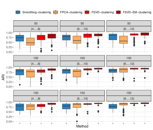
Figure 3: Box-plots of ARI values from different methods with sample sizes $n$ (main title) and numbers of time points $J_{i}$ (subtitle).

We compare the performance of FSVD in functional clustering with two existing methods: spline-clustering (James and Sugar, 2003), which employs B-spline basis functions, and FPCA-clustering (Chiou and Li, 2007; Jacques and Preda, 2013), which applies FPCA for clustering irregularly and sparsely observed functional data. For FSVD, we offer two clustering results: the initial clustering using Gaussian mixture models on FSVD outputs, referred to as FSVD-clustering; and the final clustering of the EM algorithm in Algorithm 3, referred to as FSVD-EM-clustering. For simplicity, we assume the number of clusters $H$ to be known for all methods. The clustering accuracy is evaluated by Adjusted Rand Index (ARI; Rand, 1971), which ranges from $-1$ to $1$, with higher values indicating better clustering.

Figure 3 shows box plots of ARI values from 100 simulations, where FSVD-based methods achieve superior ARIs over spline-clustering and FPCA-clustering. The lower ARIs of spline-clustering may be due to the inefficiency of B-spline bases in capturing functional patterns, while FPCA-clustering may be affected by the inaccurate estimation of subgroup covariance functions. Additionally, FSVD-EM-clustering outperforms FSVD-clustering, suggesting the value of the EM algorithm in Algorithm 3 for further improving clustering accuracy in irregularly observed functional data.

Simulations on Functional Data with Intrinsic Basis Vectors.

We further assess the performance of FSVD in estimating intrinsic basis vectors from functional data. Consider the model

$$Y_{ij}=\sum_{k=1}^{K}\rho_{k}a_{ik}F_{k}(T_{ij})+\varepsilon_{ij},\quad i\in[n],\ j\in[J_{i}],$$

where $K=3$, $\bm{A}=(a_{ik})_{i\in[n],k\in[K]}$ is a fixed loading matrix containing intrinsic basis vectors, $F_{1},\dots,F_{K}$ are random functions, $\varepsilon_{ij}$ are white noises, and $T_{ij}$ are random time points. We construct $\bm{a}_{k}$s deterministically by setting ${a}_{ik}=\sin\big{\{}k\pi(i+n/4)/(2n)\big{\}}$ for $i\in[n],k\in[K]$, letting $\bm{a}_{k}=(a_{1k},\dots,a_{nk})^{\top}$, and then orthonormalizing $\bm{a}_{k}$s by the Gram-Schmidt process. The $\rho_{k}$, $T_{ij}$, $J_{i}$, and $\varepsilon_{ij}$ are generated similarly to those in (27), and the $F_{k}$ are non-stationary series defined by $F_{k}=\sum_{g=1}^{7}c_{kg}\varphi_{g}$, where $\bm{c}_{k}=(c_{k1},\dots,c_{k7})^{\top}$ are orthonormal random vectors, and $\varphi_{g}$s are Fourier basis functions.

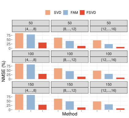
Figure 4: The $\text{NMSE}_{A}$ of different methods with sample sizes $n$ (main title) and numbers of time points $J_{i}$ (subtitle).

Using Algorithm 4, we apply FSVD to estimate the loading matrix $\bm{A}$ from the generated data. For comparison, we use matrix SVD and the method from Lam and Yao (2012); Lam et al. (2011) (denoted as FAM). The matrix SVD is equivalent to performing PCA on the time series data, assuming $\mathbb{E}Y_{ij}=0$ for all $i$ and $j$, a standard approach for estimating factor loadings (Bai and Ng, 2002). The method from Lam and Yao (2012); Lam et al. (2011) assumes the time series data to be stationary. Since these methods require observations on regular time grid, we transform the irregularly sampled simulated data onto an equally spaced time grid on $[0,1]$ with $J=\mathbb{E}J_{i}$ time points. We then set the observed data for each $t$ and $i$ as the average of $Y_{ij}$ such that $|T_{ij}-t|<0.2$ or the $Y_{ij}$ minimizing $|T_{ij}-t|$ if the former does not exist. Let $\hat{\bm{A}}=(\hat{\bm{a}}_{1},\hat{\bm{a}}_{2},\hat{\bm{a}}_{3})$ be the estimated loading matrices. To evaluate their accuracy, we define $\text{NMSE}_{A}=\min_{\bm{M}\text{ orthogonal}}\frac{\|\bm{A}-\hat{\bm{A}}\bm{M}\|^{2}}{\|\bm{A}\|^{2}}\times 100\%$, where $\bm{M}$ accounts for the fact that $\bm{A}$ is identifiable only up to a rotation.

The average NMSE values over 100 simulations are presented in Figure 4. Among the three methods, SVD performs worst due to errors from data transformation and failure to account for temporal smoothness. FAM improves upon SVD by leveraging auto-correlation, but its performance is affected by the non-stationary nature of the simulated data. Our FSVD method avoids data transformation errors and appropriately handles temporal smoothness in non-stationary time series, leading to superior performance. We also observe that the factor loadings estimated by FSVD improve as $m$ increases for different $n$, aligning with Corollary 2.

6 Real Data Analysis

In this section, we illustrate the application of FSVD using the COVID-19 case counts data from Carroll et al. (2020) and ICU electronic health record data from Johnson et al. (2024). These datasets showcase the effectiveness of FSVD in analyzing heterogeneous data from both functional and tabular perspectives.

6.1 Pattern Discovery of Epidemic Dynamic Data

Understanding the epidemic trends of COVID-19 in different regions globally is crucial for revealing outbreak patterns and assessing the effectiveness of interventions (Carroll et al., 2020; Tian et al., 2021). We analyze cumulative COVID-19 case counts per million people (in log scale) from 64 regions in 2020, collected by Dong et al. (2020). The dataset consists of case counts recorded over 67 days after each region first reported at least 20 confirmed cases. Each region’s case counts form an upward-trending trajectory and we focus on days when the cumulative case counts changed, resulting in 64 irregularly observed dynamic trajectories. For more details, see the “Methods” section in Carroll et al. (2020).

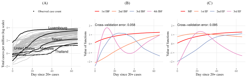
Figure 5: Panel (A): Irregularly observed time series across different regions; Panel (B): estimated intrinsic basis functions (IBFs) from FSVD; Panel (C): estimated mean function after normalization (MF) and estimated eigenfunctions (EFs) from FPCA.

In Panel (A) of Figure 5, we show the 64 trajectories from different regions. While most trajectories display a similar upward trend, some, such as Luxembourg and Thailand, have distinct rising patterns (Panel A of Figure 5), which may be due to varying regional interventions (Tian et al., 2021; Tan et al., 2022). Carroll et al. (2020) applied FPCA to these curves assuming they come from the same population. Instead, we employ FSVD to account for such heterogeneity among the regions. Panels B and C of Figure 5 display the comparison between FSVD and FPCA on the major temporal structures they extracted from the data, where FSVD is represented by the estimated intrinsic basis functions (IBFs) and FPCA is represented by the mean function and eigenfunctions. FSVD selects four components using the AIC defined in  (11), while FPCA selects three components based on the AIC proposed in Yao et al. (2005a). We can see that FSVD captures more versatile patterns than FPCA, with its 4th IBF identifying trend changes around days 15 and 35, in addition to the change around day 20 detected by both FSVD and FPCA. These additional patterns allow FSVD to better characterize regions like Thailand, Taiwan, and Luxembourg, where the timing of exponential growth and plateau phases varies.

The advantage of FSVD over FPCA is further demonstrated by its cross-validation error in functional completion. Specifically, for each region, we order its time points and split them evenly into five folds in a cyclic manner to ensure each fold has an even representation of the whole time frame. We use four folds from all regions for the estimation of FSVD components, and check the accuracy of the resulting functional completion on the remaining testing fold. We find that FSVD reduces the completion error by 39.18% compared to FPCA (errors of 0.058 for FSVD vs. 0.095 for FPCA), indicating that FSVD’s estimated functional patterns has a better representation of the data.

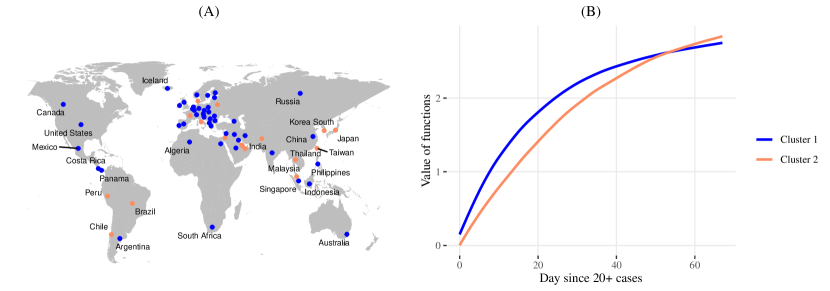
Figure 6: Panel (A): Clustering map for the dynamics from different regions; Panel (B): Estimated mean functions of two clusters from Algorithm 3.

We further apply FSVD to cluster the regions using Algorithm 3, as shown in Figure 6. Regions are grouped into two clusters (blue and yellow), with cluster 1’s mean stabilizes more quickly than that of cluster 2. These differences may reflect varying population size and intervention strategies that lead to different exponential growth and stabilization phases (Tian et al., 2021). The proposed FSVD method is able to extract both common and subgroup patterns in the trajectories of regions, thus providing valuable data-driven insights into the heterogeneity of regions in COVID-19 outbreaks.

6.2 Completion of Longitudinal Electronic Health Records

In this subsection, we use FSVD for data completion on the MIMIC-IV electronic health records dataset (Johnson et al., 2024), which contains de-identified records from ICU patients at the Beth Israel Deaconess Medical Center from 2008 to 2019. Collection times of different features are irregular and differ within each patient, making the data irregularly observed heterogeneous functional data.

For illustration purposes, we focus on 12 clinical feature data observed over 580 minutes from a single patient, as shown in Figure 7. The zero point represents the patient’s admission time to the ICU, and all features are normalized to eliminate unit effects. The definitions of the features are provided in Table 3 in the Supplementary Materials. Despite highly irregular and sparse observations across some features (e.g., Arterial O₂ Saturation, Glucose, and Neutrophils), many features exhibit smooth temporal trends. Understanding these trends and imputing missing time points by leveraging information from observed features can provide valuable insights for diagnosing and monitoring the patient’s health status.

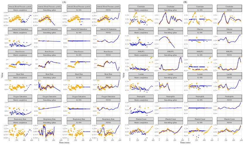
Figure 7: Data imputation/functional completion for 12 clinical features by matrix completion, smoothing spline, K-NN, and FSVD.

We compare the recovery of missing time points using FSVD with matrix completion (Candes and Plan, 2010; Candes and Recht, 2012), smoothing spline (Speckman, 1985; Gu, 2013), and a missing data imputation approach using K-NN (Bertsimas et al., 2018). For matrix completion and K-NN, we impute values only on a grid of time points $\bigcup_{i=1}^{n}\{T_{ij};j\in[J_{i}]\}$, whereas smoothing spline and FSVD allow imputation over the entire observed interval. Figure 7 shows the completion results from the four methods. We can see that matrix completion overlooks latent smoothness, leading to inaccurate completion of longitudinal clinical features. Smoothing spline, ignoring cross-function signals, is less effective in recovering trends, especially for partially observed data (e.g., Arterial Blood Pressure systolic and Heart Rate in Figure 7). K-NN preliminarily imputes missing values using the mean, likely due to the high number of missing observations from irregular data. Overall, FSVD yields more reasonable completion than the other methods by incorporating cross-functional signals and ensuring inherent smoothness.

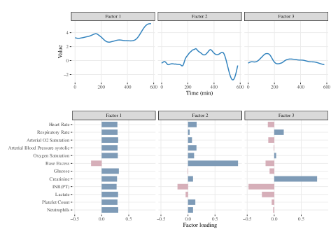
Figure 8: The estimated factor series and the corresponding factor loadings for the electronic health record from a patient.

Moreover, FSVD allows better interpretation of the results from functional completion using intrinsic basis vectors and factor models. Using the information criterion in Bai and Ng (2002), we select five latent factors from the 12 clinical features and obtain their factor loading matrix as the singular vectors from FSVD. Figure 8 presents the first three factor series and their corresponding feature loadings. The first latent factor has prominent contribution to most clinical features, with an increase around 400 minutes after ICU admission, capturing the rising trends in Platelet Count and predict similar trends in features like Heart Rate and Neutrophils (Figure 7). The second factor captures the peak of INR (PT) around 550 minute and the shift of Base Excess around 200 minute. The third primarily describes the temporary increase in Creatinine and Respiratory Rate and temporary decrease in INR(PT) and Lactate around 150 minute. By leveraging temporal correlations among clinical features, the imputed data provide a more comprehensive view of patients’ health, potentially aiding in diagnosis and guiding interventions for patients with incomplete measurements.

7 Discussions

In this article, we establish the mathematical framework, implementation procedure, and statistical theory of Functional Singular Value Decomposition (FSVD) for functional data exhibiting dependencies and heterogeneity. By introducing intrinsic basis functions and vectors, FSVD unifies various common tasks for heterogeneous functional data, providing a structure-adaptive approach for different statistical structures. We demonstrate the advantages of FSVD through extensive simulations and two data analyses, showcasing its superior performance compared to existing methods.

This paper focuses on the statistical theories of the first component of FSVD. Developing comprehensive theories for the other components and subspace estimation, especially when singular values are identical or similar, is an interesting future direction. Cai and Zhang (2018) developed sharp one-sided perturbation bounds for matrix SVD. For functional SVD, deriving separate sharp bounds for singular vectors and singular functions would be both theoretically and practically valuable. Furthermore, this article explores functional completion using FSVD under a heterogeneous functional data setting, different from methods for homogeneous functional data completion (Kraus, 2015; Kneip and Liebl, 2020) and other matrix completion, missing data imputation, and non-parametric approaches (Tsybakov, 2009; Candes and Plan, 2010; Candes and Recht, 2012; Stekhoven and Bühlmann, 2012; Gu, 2013; Bertsimas et al., 2018; Fan, 2018). A theoretical analysis comparing functional completion in our work within these methods would also be valuable.

Heterogeneous functional data with two-way heterogeneity have emerged in various real-world applications. For example, consider random functions $X_{ij}(t)$ with mean and covariance functions varying across $i$ (subjects) and (or) $j$ (features). Such data are referred to as multivariate/high-dimensional functional data (Chiou et al., 2014; Zapata et al., 2022; Hu and Yao, 2022; Li and Xiao, 2023), multivariate time series from multiple subjects (Zhang, Xue, Xu, Lee and Qu, 2024), multivariate longitudinal data (Shi et al., 2023), or functional tensors (Han et al., 2023). They exhibit complex subject-feature-function tensor structures, with irregular time grids varying across subjects or features (Shi et al., 2023; Zhang, Xue, Xu, Lee and Qu, 2024). Due to these complexities, dimension reduction is often necessary, using techniques like KL expansions (Chiou et al., 2014; Zapata et al., 2022; Hu and Yao, 2022), factor models (Li and Xiao, 2023; Zhang, Xue, Xu, Lee and Qu, 2024), and tensor SVD decompositions (Shi et al., 2023; Han et al., 2023). These methods can be considered types of singular value decomposition for functional data and may connect to our framework.

Moreover, this paper studies FSVD based on fully observed functions or discretely observed functions where the observation time points cover the entire time domain. In practice, there are scenarios where observations are available only on a fraction of the time domain. For example, Descary and Panaretos (2019); Kneip and Liebl (2020); Zhang and Chen (2022) considered covariance function estimation when functional curves are partially observed. It would be interesting to study the methodology and theory for FSVD under this observational model.

Appendix A Technical Proof

Preliminary

We first recall some notations. Let $\mathcal{T}$ be a bounded closed interval in $\mathbb{R}$. Without loss of generality, we set $\mathcal{T}$ to be $[0,1]$ throughout this article. Denote $\mathcal{L}^{2}(\mathcal{T})$ as the Hilbert space of square-integrable functions on $\mathcal{T}$ with the inner product $\langle\cdot,\cdot\rangle$ and norm $\|\cdot\|:=\sqrt{\langle\cdot,\cdot\rangle}$, where

$$\langle f,g\rangle=\int_{t\in\mathcal{T}}f(t)g(t)\ \mathrm{d}t,\ \forall f,g\in\mathcal{L}^{2}(\mathcal{T}).$$

We use $\|\cdot\|$ to denote both the Euclidean norm of a vector and the Frobenius norm of a matrix in the following proof. Denote $\overline{\mathcal{H}}$ as the closure of a set $\mathcal{H}$ from a Hilbert space in terms of its norm, and define $\operatorname{span}(f_{1},\dots,f_{n})$ as the functional space spanned by $f_{1},\dots,f_{n}\in\mathcal{L}^{2}(\mathcal{T})$. Let $\mathbb{I}(\cdot)$ be the indicator function and $[Z]$ be the set of integers $\{1,\dots,Z\}$. Moreover, we denote that $f=\lim_{n\rightarrow\infty}f_{n}$ if $\lim_{n\rightarrow\infty}\|f-f_{n}\|=0$.

Consider an operator $\mathcal{K}$ between two Hilbert spaces $\mathcal{H}_{1}$ and $\mathcal{H}_{2}$, each with inner product $\langle\cdot,\cdot\rangle_{i}$ and norms $\|\cdot\|_{i}$ for $i=1,2$. Define $\operatorname{Dom}(\mathcal{K})$ as the domain of $\mathcal{K}$. Denote $\operatorname{Im}(\mathcal{K}):=\{\mathcal{K}x;x\in\operatorname{Dom}(\mathcal{K})\}$ and $\operatorname{Null}(\mathcal{K}):=\{x\in\operatorname{Dom}(\mathcal{K});\mathcal{K}x=\bm{0}\}$ as the image and null spaces of $\mathcal{K}$, where $\bm{0}$ is the zero element in $\mathcal{H}_{2}$. Define the multiplication of two operators $\mathcal{K}_{1}$ and $\mathcal{K}_{2}$ as $\mathcal{K}_{1}\mathcal{K}_{2}$ if $\operatorname{Im}(\mathcal{K}_{2})\subset\operatorname{Dom}(\mathcal{K}_{1})$. Besides, define the operator norm of $\mathcal{K}$ as $\|\mathcal{\mathcal{K}}\|_{\infty}=\sup\{\|\mathcal{K}x\|_{2};\|x\|_{1}\leq 1\}$, and denote $\mathcal{K}^{*}$ as the adjoint operator of an operator $\mathcal{K}$ if

$$\langle\mathcal{K}f,g\rangle_{2}=\langle f,\mathcal{K}^{*}g\rangle_{1}\quad\forall f\in\mathcal{H}_{1}\text{ and }g\in\mathcal{H}_{2}.$$

Given an operator $\mathcal{K}$ from $\mathcal{H}_{1}$ to $\mathcal{H}_{1}$ such that $\|\mathcal{K}\|_{\infty}<\infty$, if there exist $e\neq 0\in\mathcal{H}_{1}$ and $\lambda\in\mathbb{R}$ obtaining

$$\mathcal{K}e=\lambda e,$$

we refer $\lambda$ and $e$ to as the eigenvalue and eigenfunction of $\mathcal{K}$, respectively.

An operator $\mathcal{K}$ is compact if for any bounded sequence $\{x_{N};N\geq 1\}$ in $\mathcal{H}_{1}$, $\{\mathcal{K}x_{N};N\geq 1\}$ has a convergent subsequence in $\mathcal{H}_{2}$. For a compact operator $\mathcal{K}$, it has the following singular value decomposition

$$\mathcal{K}f=\sum_{r=1}^{\infty}\rho_{r}\langle f,\phi_{r}\rangle_{1}\psi_{r},\ \forall f\in\mathcal{H}_{1},$$

where $\rho_{r}^{2}$ are the eigenvalues of both $\mathcal{K}^{*}\mathcal{K}$ and $\mathcal{K}\mathcal{K}^{*}$, $\{\phi_{r}\in\overline{\operatorname{Im}(\mathcal{K}^{*}\mathcal{K})};r\geq 1\}$ are the eigenfunctions of $\mathcal{K}^{*}\mathcal{K}$, and $\{\psi_{r}\in\overline{\operatorname{Im}(\mathcal{K}\mathcal{K}^{*})};r\geq 1\}$ are the eigenfunctions of $\mathcal{K}\mathcal{K}^{*}$. See Theorem 4.3.1 in Hsing and Eubank (2015) for more details.

Denote $\mathcal{H}$ as a Hilbert space of functions on $\mathcal{T}$ with inner product $\langle\cdot,\cdot\rangle_{\mathcal{H}}$ and norm $\|\cdot\|_{\mathcal{H}}$. The functional space $\mathcal{H}$ is called a reproducing kernel Hilbert space (RKHS) $\mathcal{H}(\mathbb{K})$ if there exists a kernel $\mathbb{K}$ on $\mathcal{T}\times\mathcal{T}$ such that $\mathbb{K}(t,\cdot)\in\mathcal{H}$ and

$$f(t)=\langle f,\mathbb{K}(t,\cdot)\rangle_{\mathcal{H}},$$

$\forall t\in\mathcal{T}$ and $f\in\mathcal{H}$.

For any semi-positive definite kernel $K(t,s)$ such that $\int_{0}^{1}\int_{0}^{1}(K(t,s))^{2}\ \mathrm{d}t\,\mathrm{d}s<\infty$, we call $\mathcal{K}$ an integral operator associated with $K(t,s)$ if

$$\mathcal{K}f=\int_{0}^{1}K(t,s)f(s)\ \mathrm{d}s,$$

$\forall f\in\mathcal{L}^{2}(\mathcal{T})$. It can be shown that $\mathcal{K}$ is a compact self-adjoint operator, and the SVD of $\mathcal{K}$ leads to a spectral decomposition of $K(t,s)$:

$$K(t,s)=\sum_{k=1}^{\infty}\lambda_{k}\psi_{k}(t)\psi_{k}(s),$$

where $\lambda_{k}$ and $\psi_{k}$ are the eigenvalues and eigenvectors of $\mathcal{K}$, respectively. See Section 4.6 of Hsing and Eubank (2015) for more details.

A.1 Mathematical Foundation of FSVD

A.1.1 Proof of Theorem 1

Proof.

Notice that for all $f\in\mathcal{L}^{2}(\mathcal{T})$ such that $\|f\|\leq 1$,

$$\|\mathcal{X}_{n}f\|^{2}=\sum_{i=1}^{n}\langle X_{i},f\rangle^{2}\leq\sum_{i=1}^{n}\|X_{i}\|^{2}\cdot\|f\|^{2}\leq\sum_{i=1}^{n}\|X_{i}\|^{2}.$$

Therefore, $\mathcal{X}_{n}$ is a bounded operator for any finite $n$. For any bounded sequence $\{f_{N};N\geq 1\}$ in $\mathcal{L}^{2}(\mathcal{T})$, the boundedness of $\mathcal{X}_{n}$ implies that $\{\mathcal{X}_{n}f_{N};N\geq 1\}$ is also a bounded sequence in $\mathbb{R}^{n}$. Based on the Bolzano–Weierstrass theorem, $\{\mathcal{X}_{n}f_{N};N\geq 1\}$ always has a convergent subsequence in $\mathbb{R}^{n}$. Consequently, $\mathcal{X}_{n}$ is a compact operator.

The compactness of $\mathcal{X}_{n}$ leads to the following singular value decomposition

$$\mathcal{X}_{n}f=\sum_{r=1}^{\infty}\rho_{r}\langle f,\phi_{r}\rangle\bm{a}_{r},\ \forall f\in\mathcal{L}^{2}(\mathcal{T}),$$

where $\rho_{r}^{2}$ are the eigenvalues of both $\mathcal{X}_{n}^{*}\mathcal{X}_{n}$ and $\mathcal{X}_{n}\mathcal{X}_{n}^{*}$, $\{\phi_{r}\in\overline{\operatorname{Im}(\mathcal{X}_{n}^{*}\mathcal{X}_{n})};r\geq 1\}$ are the eigenvectors of $\mathcal{X}_{n}^{*}\mathcal{X}_{n}$, and $\bm{a}_{r}$s are the eigenvectors of $\mathcal{X}_{n}\mathcal{X}_{n}^{*}$. Since $\mathcal{X}_{n}\mathcal{X}_{n}^{*}$ is a matrix in $\mathbb{R}^{n\times n}$, it follows that $\{\rho_{r};r>n\}$ are zero values. Therefore,

$$\langle X_{i},f\rangle=\sum_{r=1}^{R}\rho_{r}\langle f,\phi_{r}\rangle{a}_{ir},\ \forall f\in\mathcal{L}^{2}(\mathcal{T})\ \text{and}\ i\in[n],$$

where $R\leq n$ is the rank of $\mathcal{X}_{n}$. Therefore,

$$\mathcal{X}_{n}\phi_{r}=\big{(}\langle X_{1},\phi_{r}\rangle,\dots,\langle X_{n},\phi_{r}\rangle\big{)}^{\top}=\rho_{r}\bm{a}_{r},\ r\in[R].$$

Take $\{f_{N};N\geq 1\}$ as any orthonormal basis functions of $\mathcal{L}^{2}(\mathcal{T})$. Using the above equation, we have

$$X_{i}=\sum_{N=1}^{\infty}\langle X_{i},f_{N}\rangle f_{N}=\sum_{N=1}^{\infty}\sum_{r=1}^{R}\rho_{r}\langle f_{N},\phi_{r}\rangle{a}_{ir}f_{N}=\sum_{r=1}^{R}\rho_{r}\phi_{r}{a}_{ir},$$

for $i\in[n]$. This leads to the FSVD of $X_{i}$s.

It remains to show that $\overline{\operatorname{Im}(\mathcal{X}_{n}^{*}\mathcal{X}_{n})}\subset\mathcal{H}$ if $X_{i}\in\mathcal{H}$, $i\in[n]$. Therefore, $\mathcal{X}_{n}^{*}\mathcal{X}_{n}$ is an operator mapping from $\mathcal{H}$ to $\mathcal{H}$, and $\phi_{r}\in\mathcal{H}$, $r\in[R]$, since $\phi_{r}\in\overline{\operatorname{Im}(\mathcal{X}_{n}^{*}\mathcal{X}_{n})};r\geq 1$. By the projection theory, $\mathcal{L}^{2}(\mathcal{T})$ can be represented as

$$\mathcal{L}^{2}(\mathcal{T})=\mathcal{H}\oplus\mathcal{H}^{\perp},$$

where $\mathcal{H}^{\perp}$ is the orthogonal complement subspace of $\mathcal{H}$ in terms of the $L^{2}$ norm. As a result,

$$\mathcal{H}^{\perp}\subset\operatorname{Null}(\mathcal{X}_{n})$$

since $X_{1},\dots,X_{n}\in\mathcal{H}$. Therefore,

$$\operatorname{Null}(\mathcal{X}_{n})^{\perp}\subset(\mathcal{H}^{\perp})^{\perp}=\mathcal{H}.$$

By Theorem 3.3.7 in Hsing and Eubank (2015),

$$\operatorname{Null}(\mathcal{X}_{n})^{\perp}=\overline{\operatorname{Im}(\mathcal{X}_{n}^{*})}=\overline{\operatorname{Im}(\mathcal{X}_{n}^{*}\mathcal{X}_{n})},$$

indicating that $\overline{\operatorname{Im}(\mathcal{X}_{n}^{*}\mathcal{X}_{n})}\subset\mathcal{H}$. This in turn leads to $\phi_{r}\in\mathcal{H}$, $r\in[R]$. ∎

We present the specific expressions for $\mathcal{X}_{n}^{*}\mathcal{X}_{n}$ and $\mathcal{X}_{n}\mathcal{X}_{n}^{*}$ in Lemma 4.

A.1.2 Proof of Theorem 2

Proof.

If there exist two FSVDs of $X_{1},\ldots,X_{n}$: $\big{\{}\rho_{r},\bm{a}_{r},\phi_{r};r=1,\dots,R\big{\}}$, $\big{\{}\tilde{\rho}_{r},\tilde{\bm{a}}_{r},\tilde{\phi}_{r};r=1,\dots,\tilde{R}\big{\}}$ such that $\rho_{1}\geq\cdots\geq\rho_{R}>0$, $\tilde{\rho}_{1}\geq\cdots\geq\tilde{\rho}_{\tilde{R}}>0$, $\bm{a}_{r}^{\top}\bm{a}_{r^{\prime}}=\langle\phi_{r},\phi_{r^{\prime}}\rangle=\tilde{\bm{a}}_{r}^{\top}\tilde{\bm{a}}_{r^{\prime}}=\langle\tilde{\phi}_{r},\tilde{\phi}_{r^{\prime}}\rangle=\mathbb{I}(r=r^{\prime})$, and satisfying

$$\sum_{r=1}^{R}\rho_{r}\bm{a}_{r}\phi_{r}=\sum_{r=1}^{\tilde{R}}\tilde{\rho}_{r}\tilde{\bm{a}}_{r}\tilde{\phi}_{r}.$$

By Theorem 1, $\{\rho_{r}^{2};r\in[R]\}$ and $\{{\tilde{\rho}}_{r}^{2};r\in[\tilde{R}]\}$ are both the positive eigenvalues of $\mathcal{X}_{n}\mathcal{X}_{n}^{*}$. Therefore, $R=\tilde{R}$ and $\rho_{r}=\tilde{\rho}_{r}$ for all $r\in[R]$.

If there exists a block of identical singular values, say $\rho_{r_{1}-1}>\rho_{r_{1}}=\cdots=\rho_{r_{2}}>\rho_{r_{2}+1}$. Then $(\tilde{\bm{a}}_{r_{1}},\dots,\tilde{\bm{a}}_{r_{2}})$ and $({\bm{a}}_{r_{1}},\dots,{\bm{a}}_{r_{2}})$ are both the eigenvectors of the matrix $\mathcal{X}_{n}\mathcal{X}_{n}^{*}$ corresponding to eigenvalue $\rho_{r_{1}}$. Consequently, there exists an orthogonal matrix $\bm{B}\in\mathbb{R}^{(r_{2}-r_{1}+1)\times(r_{2}-r_{1}+1)}$ such that

$$(\tilde{\bm{a}}_{r_{1}},\dots,\tilde{\bm{a}}_{r_{2}})=({\bm{a}}_{r_{1}},\dots,{\bm{a}}_{r_{2}})\bm{B}.$$

This leads to

$$(\tilde{\phi}_{r_{1}},\dots,\tilde{\phi}_{r_{2}}) = \frac{1}{\rho_{r_{1}}}\big{(}X_{1},\dots,X_{n}\big{)}(\tilde{\bm{a}}_{r_{1}},\dots,\tilde{\bm{a}}_{r_{2}})$$

$$= \frac{1}{\rho_{r_{1}}}\big{(}X_{1},\dots,X_{n}\big{)}({\bm{a}}_{r_{1}},\dots,{\bm{a}}_{r_{2}})\bm{B}$$

$$= ({\phi}_{r_{1}},\dots,{\phi}_{r_{2}})\bm{B}.$$

We then complete the proof.

∎

A.1.3 Proof of Theorem 3

Proof.

Let $f_{i}=b_{i}g$, $i\in[n]$, for any $\bm{b}=(b_{1},\cdots,b_{n})^{\top}\in\mathbb{R}^{n}$ and $g\in\mathcal{H}$ satisfying $\|g\|=1$. Denote

$$X_{i}=\sum_{r=1}^{R}\rho_{r}^{0}a^{0}_{ir}\phi_{r}^{0}$$

as the FSVD of $X_{i}$s, where $\rho_{1}^{0}\geq\rho_{2}^{0}\geq\dots\geq\rho_{R}^{0}$. Note that

$$L(\bm{b},g): = \sum_{i=1}^{n}\|X_{i}-f_{i}\|^{2}=\sum_{i=1}^{n}\|X_{i}\|^{2}-2\sum_{i=1}^{n}{b_{i}}\langle X_{i},g\rangle+\sum_{i=1}^{n}b_{i}^{2}$$

$$= \sum_{i=1}^{n}\|X_{i}\|^{2}-2\sum_{i=1}^{n}\sum_{r=1}^{R}\rho_{r}^{0}a^{0}_{ir}b_{i}\langle\phi_{r}^{0},g\rangle+\sum_{i=1}^{n}b_{i}^{2}$$

$$= \sum_{i=1}^{n}\|X_{i}\|^{2}-2\sum_{r=1}^{R}\rho_{r}^{0}\langle\bm{a}_{r}^{0},\bm{b}\rangle\langle\phi_{r}^{0},g\rangle+\sum_{i=1}^{n}b_{i}^{2}.$$

Since $\sum_{r=1}^{R}\langle\bm{a}_{r}^{0},\bm{b}\rangle^{2}\leq\|\bm{b}\|^{2}$ and $\sum_{r=1}^{R}\langle\phi_{r}^{0},g\rangle^{2}\leq 1$,

$$\sum_{r=1}^{R}\big{|}\langle\bm{a}_{r}^{0},\bm{b}\rangle\langle\phi_{r}^{0},g\rangle\big{|}\leq\|\bm{b}\|.$$

This leads to that

$$\sum_{r=1}^{R}\rho_{r}^{0}\langle\bm{a}_{r}^{0},\bm{b}\rangle\langle\phi_{r}^{0},g\rangle\leq\sup_{r\in[R]}\{\rho_{r}^{0}\}\sum_{r=1}^{R}\big{|}\langle\bm{a}_{r}^{0},\bm{b}\rangle\langle\phi_{r}^{0},g\rangle\big{|}\leq\rho_{1}^{0}\|\bm{b}\|.$$

Then for any $\bm{b}$ and $g$,

$$L(\bm{b},g)\geq\sum_{i=1}^{n}\|X_{i}\|^{2}-2\rho_{1}^{0}\|\bm{b}\|+\|\bm{b}\|^{2}=L(\|\bm{b}\|\bm{a}_{1}^{0},\phi^{0}_{1}).$$

Using the fact that $-2\rho_{1}^{0}d+d^{2}\geq-(\rho_{1}^{0})^{2}$, we have

$$L(\bm{b},g)\geq\sum_{i=1}^{n}\|X_{i}\|^{2}-(\rho_{1}^{0})^{2}=L(\rho_{1}^{0}\bm{a}_{1}^{0},\phi^{0}_{1}),$$

and “$=$” holds if $\bm{b}=\rho_{1}^{0}\bm{a}_{1}^{0}$ and $g=\phi^{0}_{1}$. We then obtain

$$(\rho_{1}^{0}a_{11}^{0}\phi^{0}_{1},\dots,\rho_{1}^{0}a^{0}_{n1}\phi^{0}_{1})=\operatorname*{arg\,min}_{f_{1},\dots,f_{n}\in\mathcal{H}}\sum_{i=1}^{n}\|X_{i}-f_{i}\|^{2}\quad\text{subject to}\quad\operatorname{dim}(f_{1},\dots,f_{n})=1.$$

For $R>1$, notice that

$$X_{i}-\sum_{l=1}^{r-1}g_{ir}=\sum_{l=r}^{R}{\rho}_{l}^{0}a_{il}^{0}{\phi}_{l}^{0},$$

where $g_{ir}=\rho_{r}^{0}a_{1r}^{0}\phi_{r}^{0}$. We similarly prove that $({\rho}_{r}^{0},{\bm{a}}_{r}^{0},{\phi}_{r}^{0})$ is the minimizer of the optimization

$$(\rho_{r}^{0}a_{1r}^{0}\phi_{r}^{0},\dots,\rho_{r}^{0}a^{0}_{nr}\phi^{0}_{r})=\operatorname*{arg\,min}_{f_{1},\dots,f_{n}\in\mathcal{H}}\sum_{i=1}^{n}\bigg{\|}X_{i}-\sum_{l=1}^{r-1}g_{ir}-f_{i}\bigg{\|}^{2}\quad\text{subject to}\quad\operatorname{dim}(f_{1},\dots,f_{n})=1.$$

for $r>1$. ∎

A.1.4 Proof of Theorem 4

Proof.

Define

$$L(\bm{a},\phi):=\sum_{i=1}^{n}\frac{1}{J_{i}}\sum_{j=1}^{J_{i}}\big{\{}Y_{ij}-a_{i}\phi(T_{ij})\big{\}}^{2}+\nu\|\bm{a}\|^{2}\cdot\|\mathcal{P}\phi\|_{\mathcal{H}}^{2},$$

and

$$\mathcal{H}:=\bigg{\{}f\in\mathcal{H}(\mathbb{K});\ f=\sum_{m=1}^{q}{u}_{m}h_{m}+\sum_{i=1}^{n}\sum_{j=1}^{J_{i}}{w}_{ij}g_{ij},\ u_{m}\in\mathbb{R},\ w_{ij}\in\mathbb{R}\bigg{\}}.$$

Since

$$\mathbb{K}(\cdot,T_{ij})=\mathbb{K}(\cdot,T_{ij})-\mathcal{P}\big{\{}\mathbb{K}(\cdot,T_{ij})\big{\}}+g_{ij},$$

where $\mathbb{K}(\cdot,T_{ij})-\mathcal{P}\big{\{}\mathbb{K}(\cdot,T_{ij})\big{\}}\in\text{Null}(\mathcal{P})\subset\mathcal{H}$ and $g_{ij}\in\mathcal{H}$, then $\mathbb{K}(\cdot,T_{ij})\in\mathcal{H}$.

Let $\mathcal{H}(\mathbb{K})=\mathcal{H}\oplus\mathcal{H}^{\perp}$, where $\mathcal{H}^{\perp}$ is the orthogonal complement subspace of $\mathcal{H}$ in terms of its inner product. For any $f\in\mathcal{H}(\mathbb{K})$, we can separate it as

$$f=\phi+\phi^{\perp}_{1},$$

where $\phi\in\mathcal{H}$ and $\phi^{\perp}_{1}\in\mathcal{H}^{\perp}$. As a result,

$$f(T_{ij}) = \phi(T_{ij})+\phi^{\perp}_{1}(T_{ij})$$ (28)

$$= \phi(T_{ij})+\langle\phi^{\perp}_{1},\mathbb{K}(\cdot,T_{ij})\rangle_{\mathcal{H}}$$

$$= \phi(T_{ij})$$

due to $\mathbb{K}(\cdot,T_{ij})\in\mathcal{H}$.

Moreover, note that the projected function $\phi$ for $f$ can be represented by $\sum_{m=1}^{q}{u}_{m}h_{m}+\sum_{i=1}^{n}\sum_{j=1}^{J_{i}}{w}_{ij}g_{ij}$. Since $\mathcal{P}\phi=\sum_{i=1}^{n}\sum_{j=1}^{J_{i}}{w}_{ij}\mathcal{P}g_{ij}=\sum_{i=1}^{n}\sum_{j=1}^{J_{i}}{w}_{ij}g_{ij}\in\mathcal{H}$, we have

$$\langle\mathcal{P}\phi,\mathcal{P}\phi^{\perp}_{1}\rangle=\langle\mathcal{P}^{2}\phi,\phi^{\perp}_{1}\rangle=\langle\mathcal{P}\phi,\phi^{\perp}_{1}\rangle=0.$$

Therefore,

$$\|\mathcal{P}f\|^{2}=\|\mathcal{P}\phi+\mathcal{P}\phi^{\perp}_{1}\|^{2}\geq\|\mathcal{P}\phi\|^{2}.$$ (29)

Combining with (28) and (29), we have that $\forall\bm{a}\in\mathbb{R}^{n}\ \text{and}\ f\in\mathcal{H}(\mathbb{K})$, there always exists a projected function $\phi$ of $f$ onto $\mathcal{H}$ such that

$$L(\bm{a},f)\geq L(\bm{a},\phi).$$

We then complete the proof. ∎

A.2 Equivalences of Intrinsic Basis Functions/Vectors

A.2.1 Proof of Theorem 6

Proof.

Observe that $H_{n}(t,s):=\frac{1}{n}\mathbb{E}\sum_{i=1}^{n}X_{i}(t)X_{i}(s)$ is always a non-negative-definite kernel.

(a) $\Rightarrow$ (b): Notice that

$$\sum_{i=1}^{n}\mathbb{E}\bigg{\|}X_{i}-\sum_{k=1}^{K}{\xi}_{ik}{\varphi}_{k}\bigg{\|}^{2}=n\cdot\bigg{(}\int_{0}^{1}H_{n}(t,t)\ \mathrm{d}t-\sum_{k=1}^{K}\int_{0}^{1}\int_{0}^{1}H_{n}(t,s){\varphi}_{k}(t){\varphi}_{k}(s)\ \mathrm{d}t\,\mathrm{d}s\bigg{)}.$$

Let $H_{n}(t,s)=\sum_{k=1}^{\infty}\lambda_{k}\tilde{\varphi}_{k}(t)\tilde{\varphi}_{k}(s)$, where $\lambda_{1}\geq\lambda_{2}\geq\cdots\geq 0$ are eigenvalues, and $\tilde{\varphi}_{k}$s are eigenfunctions. Consequently, the above equation can be represented by

$$\frac{1}{n}\sum_{i=1}^{n}\mathbb{E}\bigg{\|}X_{i}-\sum_{k=1}^{K}{\xi}_{ik}{\varphi}_{k}\bigg{\|}^{2}=\sum_{k=1}^{\infty}\lambda_{k}-\sum_{k=1}^{K}\lambda_{k}\langle{\varphi}_{k},\tilde{\varphi}_{k}\rangle^{2}.$$

Therefore, $\langle{\varphi}_{k},\tilde{\varphi}_{k}\rangle^{2}=1$ for all $k\geq 1$. Otherwise, there exists some $K$ such that

$$\sum_{i=1}^{n}\mathbb{E}\bigg{\|}X_{i}-\sum_{k=1}^{K}\tilde{\xi}_{ik}\tilde{\varphi}_{k}\bigg{\|}^{2}=\sum_{k=K+1}^{\infty}\lambda_{k}\leq\sum_{i=1}^{n}\mathbb{E}\bigg{\|}X_{i}-\sum_{k=1}^{K}{\xi}_{ik}{\varphi}_{k}\bigg{\|}^{2},$$

where $\tilde{\xi}_{ik}=\langle X_{i},\tilde{\varphi}_{k}\rangle$. This is a contradiction to (a). We then conclude that the $\varphi_{k}$s are the eigenfunctions of $H_{n}(t,s)$.

(b) $\Rightarrow$ (c): If $\{\varphi_{k};k\geq 1\}$ are the eigenfunctions of $H_{n}(t,s)$, then

$$\sum_{i=1}^{n}\mathbb{E}\xi_{ik_{1}}\xi_{ik_{2}} = \sum_{i=1}^{n}\mathbb{E}\int_{\mathcal{T}}\int_{\mathcal{T}}X_{i}(t)X_{i}(s)\varphi_{k_{1}}(t)\varphi_{k_{2}}(s)\ \mathrm{d}t\,\mathrm{d}s$$

$$= n\int_{\mathcal{T}}\int_{\mathcal{T}}H_{n}(t,s)\varphi_{k_{1}}(t)\varphi_{k_{2}}(s)\ \mathrm{d}t\,\mathrm{d}s.$$

As a result, $\sum_{i=1}^{n}\mathbb{E}\xi_{ik_{1}}\xi_{ik_{2}}=0$ if $k_{1}\neq k_{2}$.

(c) $\Rightarrow$ (a): Recall that $\{\tilde{\varphi}_{k};k\geq 1\}$ are any orthonormal basis functions in $\mathcal{L}^{2}(\mathcal{T})$ and $\tilde{\xi}_{ik}$s are any random variables. Without loss of generality, we assume that $\sum_{i=1}^{n}\mathbb{E}\big{\|}X_{i}-\sum_{k=1}^{K}\tilde{\xi}_{ik}\tilde{\varphi}_{k}\big{\|}^{2}$ is finite. Notice that

$$\bigg{\|}X_{i}-\sum_{k=1}^{K}\langle X_{i},\tilde{\varphi}_{k}\rangle\tilde{\varphi}_{k}\bigg{\|}^{2}\leq\bigg{\|}X_{i}-\sum_{k=1}^{K}\tilde{\xi}_{ik}\tilde{\varphi}_{k}\bigg{\|}^{2},\ \text{a.s.}$$

Consequently,

$$\sum_{i=1}^{n}\mathbb{E}\bigg{\|}X_{i}-\sum_{k=1}^{K}\langle X_{i},\tilde{\varphi}_{k}\rangle\tilde{\varphi}_{k}\bigg{\|}^{2}\leq\sum_{i=1}^{n}\mathbb{E}\bigg{\|}X_{i}-\sum_{k=1}^{K}\tilde{\xi}_{ik}\tilde{\varphi}_{k}\bigg{\|}^{2}.$$

We now show that

$$\sum_{i=1}^{n}\mathbb{E}\bigg{\|}X_{i}-\sum_{k=1}^{K}{\xi}_{ik}{\varphi}_{k}\bigg{\|}^{2}\leq\sum_{i=1}^{n}\mathbb{E}\bigg{\|}X_{i}-\sum_{k=1}^{K}\langle X_{i},\tilde{\varphi}_{k}\rangle\tilde{\varphi}_{k}\bigg{\|}^{2},$$

where $\tilde{\xi}_{ik}$ is taken as $\langle X_{i},\tilde{\varphi}_{k}\rangle$, $\forall i\in[n]$ and $k\geq 1$.

Note that

$$\sum_{i=1}^{n}\mathbb{E}\bigg{\|}X_{i}-\sum_{k=1}^{K}\tilde{\xi}_{ik}\tilde{\varphi}_{k}\bigg{\|}^{2}=\sum_{i=1}^{n}\mathbb{E}\|X_{i}\|^{2}-\sum_{k=1}^{K}\sum_{i=1}^{n}\mathbb{E}\langle X_{i},\tilde{\varphi}_{k}\rangle^{2}.$$

Represent $\tilde{\varphi}_{k}=\sum_{g=1}^{\infty}\langle\tilde{\varphi}_{k},{\varphi}_{g}\rangle\varphi_{g}:=\sum_{g=1}^{\infty}a_{gk}\varphi_{g}$. Therefore,

$$\sum_{i=1}^{n}\mathbb{E}\langle X_{i},\tilde{\varphi}_{k}\rangle^{2}=\sum_{i=1}^{n}\mathbb{E}\bigg{\langle}X_{i},\sum_{g=1}^{\infty}a_{gk}\varphi_{g}\bigg{\rangle}^{2}=\sum_{i=1}^{n}\mathbb{E}\bigg{(}\sum_{g=1}^{\infty}a_{gk}\xi_{ig}\bigg{)}^{2}=\sum_{g=1}^{\infty}a_{gk}^{2}\sum_{i=1}^{n}\mathbb{E}\xi_{ig}^{2}.$$

We claim that

$$\sum_{k=1}^{K}\sum_{g=1}^{\infty}a_{gk}^{2}\sum_{i=1}^{n}\mathbb{E}\xi_{ig}^{2}\leq\sum_{k=1}^{K}\sum_{i=1}^{n}\mathbb{E}\xi_{ik}^{2},$$ (30)

which implies

$$\sum_{i=1}^{n}\mathbb{E}\bigg{\|}X_{i}-\sum_{k=1}^{K}\xi_{ik}\varphi_{k}\bigg{\|}^{2}\leq\sum_{i=1}^{n}\mathbb{E}\bigg{\|}X_{i}-\sum_{k=1}^{K}\tilde{\xi}_{ik}\tilde{\varphi}_{k}\bigg{\|}^{2}.$$

To prove (30), note that

$$\sum_{g=1}^{\infty}a_{gk}^{2}\sum_{i=1}^{n}\mathbb{E}\xi_{ig}^{2} = \sum_{i=1}^{n}\mathbb{E}\xi_{iK}^{2}+\bigg{(}\sum_{g=1}^{K}a_{gk}^{2}\sum_{i=1}^{n}\mathbb{E}\xi_{ig}^{2}-\sum_{i=1}^{n}\mathbb{E}\xi_{iK}^{2}\sum_{g=1}^{K}a_{gk}^{2}\bigg{)}$$

$$\ -\bigg{(}\sum_{i=1}^{n}\mathbb{E}\xi_{iK}^{2}\sum_{g>K}a^{2}_{gk}-\sum_{g>K}a_{gk}^{2}\sum_{i=1}^{n}\mathbb{E}\xi_{ig}^{2}\bigg{)}$$

$$= \sum_{i=1}^{n}\mathbb{E}\xi_{iK}^{2}+\bigg{\{}\sum_{g=1}^{K}a_{gk}^{2}\bigg{(}\sum_{i=1}^{n}\mathbb{E}\xi_{ig}^{2}-\sum_{i=1}^{n}\mathbb{E}\xi_{iK}^{2}\bigg{)}\bigg{\}}$$

$$\ +\bigg{\{}\sum_{g>K}a^{2}_{gk}\bigg{(}\sum_{i=1}^{n}\mathbb{E}\xi_{ig}^{2}-\sum_{i=1}^{n}\mathbb{E}\xi_{iK}^{2}\bigg{)}\bigg{\}},$$

where the term $\bigg{\{}\sum_{g>K}a^{2}_{gk}\bigg{(}\sum_{i=1}^{n}\mathbb{E}\xi_{ig}^{2}-\sum_{i=1}^{n}\mathbb{E}\xi_{iK}^{2}\bigg{)}\bigg{\}}$ is nonpositive since $\sum_{i=1}^{n}\mathbb{E}\xi_{ik}^{2}$ decreases as $k$ increases. Therefore,

$$\sum_{k=1}^{K}\sum_{g=1}^{\infty}a_{gk}^{2}\sum_{i=1}^{n}\mathbb{E}\xi_{ig}^{2} \leq K\sum_{i=1}^{n}\mathbb{E}\xi_{iK}^{2}+\bigg{(}\sum_{k=1}^{K}\sum_{g=1}^{K}a_{gk}^{2}\bigg{(}\sum_{i=1}^{n}\mathbb{E}\xi_{ig}^{2}-\sum_{i=1}^{n}\mathbb{E}\xi_{iK}^{2}\bigg{)}\bigg{)}$$

$$= K\sum_{i=1}^{n}\mathbb{E}\xi_{iK}^{2}+\bigg{(}\sum_{g=1}^{K}\bigg{(}\sum_{i=1}^{n}\mathbb{E}\xi_{ig}^{2}-\sum_{i=1}^{n}\mathbb{E}\xi_{iK}^{2}\bigg{)}\cdot\bigg{(}\sum_{k=1}^{K}a_{gk}^{2}\bigg{)}\bigg{)}$$

$$\leq \sum_{g=1}^{K}\bigg{\{}\sum_{i=1}^{n}\mathbb{E}\xi_{iK}^{2}+\bigg{(}\sum_{i=1}^{n}\mathbb{E}\xi_{ig}^{2}-\sum_{i=1}^{n}\mathbb{E}\xi_{iK}^{2}\bigg{)}\cdot 1\bigg{\}}$$

$$= \sum_{g=1}^{K}\sum_{i=1}^{n}\mathbb{E}\xi_{ig}^{2}.$$

In the last inequality, we use the fact that $\sum_{k=1}^{K}a_{gk}^{2}\leq 1$ since $\tilde{\varphi}_{k}$s are orthonormal functions. Claim holds.

∎

A.2.2 Proof of Theorem 8

Proof.

Note that for any $\tilde{\bm{L}}\in\mathbb{R}^{n\times K}$ with orthonormal columns and any random function $\tilde{\bm{F}}(t)\in\mathbb{R}^{K}$, we have

$$\big{\|}\bm{X}(t)-\tilde{\bm{L}}\bm{G}(t)\big{\|}^{2}\leq\big{\|}\bm{X}(t)-\tilde{\bm{L}}\tilde{\bm{F}}(t)\big{\|}^{2},\ \text{almost surely},$$

for each $t$, where $\bm{G}(t)=\tilde{\bm{L}}^{\top}\bm{X}(t)$. This is because $\bm{G}(t)$ minimizes the expression $\big{\|}\bm{X}(t)-\tilde{\bm{L}}\bm{G}(t)\big{\|}^{2}$ with respect to $\bm{G}(t)$ for each $t$. Therefore,

$$\int_{\mathcal{T}}\mathbb{E}\big{\|}\bm{X}(t)-\tilde{\bm{L}}\bm{G}(t)\big{\|}^{2}\ \mathrm{d}t\leq\int_{\mathcal{T}}\mathbb{E}\big{\|}\bm{X}(t)-\tilde{\bm{L}}\tilde{\bm{F}}(t)\big{\|}^{2}\ \mathrm{d}t.$$

This leads to

$$\int_{\mathcal{T}}\mathbb{E}\big{\|}\bm{X}(t)-{\bm{L}}\bm{F}(t)\big{\|}^{2}\ \mathrm{d}t\leq\int_{\mathcal{T}}\mathbb{E}\big{\|}\bm{X}(t)-\tilde{\bm{L}}{\bm{G}}(t)\big{\|}^{2}\ \mathrm{d}t,$$

where $\bm{L}$ has orthonormal columns and represents the intrinsic basis vectors, and $\bm{F}(t)=\bm{{L}}^{\top}\bm{X}(t)$. Since

$$\mathbb{E}\big{\|}\bm{X}(t)-\tilde{\bm{L}}\bm{G}(t)\big{\|}^{2} = \mathbb{E}\|\bm{X}(t)\|^{2}-\mathbb{E}\big{[}\bm{X}^{\top}(t)\tilde{\bm{L}}\tilde{\bm{L}}^{\top}\bm{X}(t)\big{]}$$ (31)

$$= \operatorname{tr}\left(\mathbb{E}\big{[}\bm{X}(t)\bm{X}^{\top}(t)\big{]}\left(\bm{I}-\tilde{\bm{L}}\tilde{\bm{L}}^{\top}\right)\right),$$

we then have

$$\operatorname{tr}\left(\left(\int_{\mathcal{T}}\mathbb{E}\big{[}\bm{X}(t)\bm{X}^{\top}(t)\big{]}\ \mathrm{d}t\right)\left(\bm{I}-\bm{L}\bm{L}^{\top}\right)\right)\leq\operatorname{tr}\left(\left(\int_{\mathcal{T}}\mathbb{E}\big{[}\bm{X}(t)\bm{X}^{\top}(t)\big{]}\ \mathrm{d}t\right)\left(\bm{I}-\tilde{\bm{L}}\tilde{\bm{L}}^{\top}\right)\right),$$

or equivalently,

$$\operatorname{tr}\left(\bm{L}^{\top}\left(\int_{\mathcal{T}}\mathbb{E}\big{[}\bm{X}(t)\bm{X}^{\top}(t)\big{]}\ \mathrm{d}t\right)\bm{L}\right)\geq\operatorname{tr}\left(\tilde{\bm{L}}^{\top}\left(\int_{\mathcal{T}}\mathbb{E}\big{[}\bm{X}(t)\bm{X}^{\top}(t)\big{]}\ \mathrm{d}t\right)\tilde{\bm{L}}\right),$$

for any $\tilde{\bm{L}}$. This implies that $\bm{L}$ maximizes the projected variance. Consequently, there exists an orthogonal matrix $\bm{B}\in\mathbb{R}^{K\times K}$ such that $\bm{L}\bm{B}$ consists of the first $K$ eigenvectors of $\int_{\mathcal{T}}\mathbb{E}\big{[}\bm{X}(t)\bm{X}^{\top}(t)\big{]}\ \mathrm{d}t$. ∎

A.2.3 Proof of Theorem 9

Proof.

(a) $\Rightarrow$ (b): Note that $K$ is the rank of $\int_{\mathcal{T}}\mathbb{E}\bm{X}(t)\bm{X}^{\top}(t)\ \mathrm{d}t$. By Theorem 8, we have that

$$\int_{0}^{1}\mathbb{E}\bm{X}(t)\bm{X}^{\top}(t)\ \mathrm{d}t=\bm{L}\bm{B}\bm{\Lambda}\bm{B}^{\top}\bm{L}^{\top},$$

where $\bm{\Lambda}\in\mathbb{R}^{K\times K}$ is a diagonal matrix with its diagonal elements being the positive eigenvalues of $\int_{0}^{1}\mathbb{E}\bm{X}(t)\bm{X}^{\top}(t)\ \mathrm{d}t$.

Therefore, there exists a positive-definite matrix $\bm{A}\in\mathbb{R}^{K\times K}$ such that

$$\int_{0}^{1}\mathbb{E}\bm{X}(t)\bm{X}^{\top}(t)\ \mathrm{d}t=\bm{L}\bm{A}\bm{L}^{\top}.$$

By (31),

$$\mathbb{E}\int_{0}^{1}\big{\|}\bm{X}(t)-\bm{L}\bm{F}(t)\big{\|}^{2}\ \mathrm{d}t=\int_{0}^{1}\mathbb{E}\big{\|}\bm{X}(t)-\bm{L}\bm{F}(t)\big{\|}^{2}\ \mathrm{d}t=\operatorname{tr}\bigg{\{}\bm{L}\bm{A}\bm{L}^{\top}\bigg{(}\bm{I}-\bm{L}\bm{L}^{\top}\bigg{)}\bigg{\}}=0.$$

This in turn leads to

$$\bm{X}(t)=\bm{L}\bm{F}(t),\ t\in\mathcal{S},$$

almost surely, where $\mathcal{S}\subset[0,1]$ has Lebesgue measure one.

(b) $\Rightarrow$ (c): By (b), we have

$$\int_{\mathcal{T}}\bm{X}(t)\bm{X}^{\top}(t)\ \mathrm{d}t=\int_{\mathcal{S}}\bm{X}(t)\bm{X}^{\top}(t)\ \mathrm{d}t=\bm{L}\bigg{(}\int_{\mathcal{S}}\bm{F}(t)\bm{F}^{\top}(t)\ \mathrm{d}t\bigg{)}\bm{L}^{\top},$$ (32)

almost surely. Let us consider the eigendecomposition of $\int_{\mathcal{S}}\bm{F}(t)\bm{F}^{\top}(t)\ \mathrm{d}t=\bm{B}\bm{\Lambda}\bm{B}^{\top}$, where $\bm{B}\in\mathbb{R}^{K\times H}$ and $\bm{\Lambda}\in\mathbb{R}^{H\times H}$ is diagonal, we have

$$\int_{\mathcal{T}}\bm{X}(t)\bm{X}^{\top}(t)\ \mathrm{d}t=\bm{L}\bm{B}\bm{\Lambda}\bm{B}^{\top}\bm{L}^{\top},$$ (33)

almost surely, where $\bm{B}\in\mathbb{R}^{K\times H}$ and $\bm{\Lambda}\in\mathbb{R}^{H\times H}$, with $H=\operatorname{rank}\left(\int_{\mathcal{S}}\bm{F}(t)\bm{F}^{\top}(t)\ \mathrm{d}t\right)$. Recall that $R$ is the rank of $\int_{\mathcal{T}}\bm{X}(t)\bm{X}^{\top}(t)\ \mathrm{d}t$ due to Theorem 1 and Lemma 4. By (32), we have that $R\leq H$. Since $\bm{F}(t)=\bm{L}^{\top}\bm{X}(t)$,

$$\int_{\mathcal{S}}\bm{F}(t)\bm{F}^{\top}(t)\ \mathrm{d}t=\bm{L}^{\top}\bigg{(}\int_{\mathcal{T}}\bm{X}(t)\bm{X}^{\top}(t)\ \mathrm{d}t\bigg{)}\bm{L},$$

almost surely. Therefore, $H\leq R$, almost surely. We then have $H=R$, almost surely.

By Lemma 4,

$$\int_{\mathcal{T}}\bm{X}(t)\bm{X}^{\top}(t)\ \mathrm{d}t=\mathcal{X}_{n}\mathcal{X}_{n}^{*},$$

where $\mathcal{X}_{n}$ is defined in (3) in the main text. Therefore, the eigenvectors of $\int_{\mathcal{T}}\bm{X}(t)\bm{X}^{\top}(t)\ \mathrm{d}t$, which are $\bm{L}\bm{B}$ due to (33), are the singular vectors of $X_{i}$s due to Theorem 1. As such, $\bm{L}\bm{B}$ are the singular vectors of $X_{i}$s, almost surely.

We next prove that $R\leq K$, almost surely. Take any vector $\bm{b}\in\mathbb{R}^{n}$ such that $\bm{b}^{\top}\bigg{(}\int_{\mathcal{T}}\mathbb{E}\bm{X}(t)\bm{X}^{\top}(t)\ \mathrm{d}t\bigg{)}\bm{b}=0$. Since $\int_{\mathcal{T}}\bm{X}(t)\bm{X}^{\top}(t)\ \mathrm{d}t$ is a semi-positive definite matrix, then

$$\bm{b}^{\top}\bigg{(}\int_{\mathcal{T}}\bm{X}(t)\bm{X}^{\top}(t)\ \mathrm{d}t\bigg{)}\bm{b}\geq 0.$$

Combining with the above facts, $\bm{b}^{\top}\bigg{(}\int_{\mathcal{T}}\bm{X}(t)\bm{X}^{\top}(t)\ \mathrm{d}t\bigg{)}\bm{b}=0$, almost surely, which leads to

$$\operatorname{null}\bigg{(}\int_{\mathcal{T}}\mathbb{E}\bm{X}(t)\bm{X}^{\top}(t)\ \mathrm{d}t\bigg{)}\subset\operatorname{null}\bigg{(}\int_{\mathcal{T}}\bm{X}(t)\bm{X}^{\top}(t)\ \mathrm{d}t\bigg{)},$$

where $\operatorname{null}(\cdot)$ indicates the null space of a matrix. Therefore, $R\leq K$, almost surely.

(c) $\Rightarrow$ (a): By (c), there exist a diagonal matrix $\bm{\Lambda}\in\mathbb{R}^{R\times R}$ and $\bm{B}\in\mathbb{R}^{K\times R}$ such that

$$\int_{\mathcal{T}}\bm{X}(t)\bm{X}^{\top}(t)\ \mathrm{d}t=\bm{L}\bm{B}\bm{\Lambda}\bm{B}^{\top}\bm{L}^{\top},$$

almost surely. Therefore,

$$\int_{\mathcal{T}}\mathbb{E}\bm{X}(t)\bm{X}^{\top}(t)\ \mathrm{d}t=\bm{L}\big{(}\mathbb{E}\bm{B}\bm{\Lambda}\bm{B}^{\top}\big{)}\bm{L}^{\top}.$$

By the eigendecomposition of $\mathbb{E}\bm{B}\bm{\Lambda}\bm{B}^{\top}$, we then prove that $\bm{L}$ are the intrinsic basis vectors of $X_{i}$s due to Theorem 8. ∎

A.3 Statistical Convergences of FSVD

A.3.1 Proof of Theorem 5

Before proving Theorem 5, we assume that

$$\sqrt{\sum_{i=1}^{n}\bigg{(}\frac{1}{J_{i}}\sum_{j=1}^{J_{i}}f_{i}(T_{ij})-\int_{0}^{1}f_{i}(t)\ \mathrm{d}t\bigg{)}^{2}} \lesssim m^{-q/(2q+1)}\cdot\sqrt{\sum_{i=1}^{n}\|f_{i}\|^{2}}+m^{-2q/(2q+1)}\cdot\sqrt{\sum_{i=1}^{n}\|f_{i}\|_{\infty}^{2}},$$ (34)

$$\sup_{i\in[n]}\bigg{|}\frac{1}{J_{i}}\sum_{j=1}^{J_{i}}f_{i}(T_{ij})-\int_{0}^{1}f_{i}(t)\ \mathrm{d}t\bigg{|} \lesssim m^{-q/(2q+1)}\cdot\sup_{i\in[n]}\|f_{i}\|+m^{-2q/(2q+1)}\cdot\sup_{i\in[n]}\|f_{i}\|_{\infty},$$ (35)

$$\sum_{i=1}^{n}\frac{1}{J_{i}}\sum_{j=1}^{J_{i}}|\varepsilon_{ij}| \lesssim x\sqrt{\frac{n}{m}}\cdot\sigma,$$ (36)

$$\sum_{i=1}^{n}\frac{a_{i1}^{0}}{J_{i}}\sum_{j=1}^{J_{i}}|\varepsilon_{ij}| \lesssim x\sqrt{\frac{1}{m}}\cdot\sigma,$$ (37)

where $f_{i}\in\mathcal{W}_{2}^{q}(\mathcal{T})$, $i\in[n]$, are any functions such that $\sup_{i\in[n]}\|f_{i}\|\lesssim 1$, $x$ is any positive real value, and we use the notation $\|\cdot\|_{\infty}$ to denote a norm for a function $f$ defined by $\|f\|_{\infty}=\sup_{t\in\mathcal{T}}|f(t)|$.

The inequalities (34) – (37) hold with a probability at least $1-C_{1}\exp(-C_{2}m^{\frac{1}{2q+1}})-2\exp(-x^{2}/2)$ under Assumptions 1, 2, and 4. Refer to Lemmas 5 and 6 for detailed proofs.

Under the conditions (34) – (37), we propose the following three lemmas to prove Theorem 5.

Lemma 1.

Under Assumptions 1 – 4, and conditions (34) – (37), suppose that $\|\widehat{\rho\phi}^{(h)}\|\lesssim\rho_{1}^{0}$. Then

$$\operatorname{dist}(\hat{\bm{a}}^{(h+1)},{\bm{a}}_{1}^{0}) \leq C\bigg{(}m^{-q/(2q+1)}+\sqrt{\frac{n}{m}}\frac{\sigma}{\rho_{1}^{0}}\cdot x+\frac{1}{\rho_{1}^{0}}\big{\|}\overline{\rho\phi}^{(h)}-\widehat{\rho\phi}^{(h)}\big{\|}\bigg{)}$$ (38)

$$+ \operatorname{dist}^{2}(\hat{\bm{a}}^{(h)},{\bm{a}}_{1}^{0})+\frac{1}{\kappa^{2}}\operatorname{dist}(\hat{\bm{a}}^{(h)},{\bm{a}}_{1}^{0}),$$

where $\overline{\rho\phi}^{(h)}=\sum_{i=1}^{n}\hat{a}^{(h)}_{i}X_{i}$.

Lemma 2.

Under Assumptions 1 – 4 and conditions (34) – (37), we assume that the tuning parameter $\nu$ satisfies $\frac{1}{\nu^{1/(4q)}}\cdot\frac{\sigma}{\rho_{1}^{0}\sqrt{m}}\cdot x+\sqrt{\nu}\lesssim 1$ and $m^{-q/(2q+1)}+\sqrt{\frac{n}{m}}\frac{\sigma}{\rho_{1}^{0}}\cdot x\lesssim\nu^{1/(2q)}$ for a fixed $x>0$. Then

$$\|\overline{\rho\phi}^{(h)}-\widehat{\rho\phi}^{(h)}\| \lesssim \rho_{1}^{0}\bigg{(}\frac{1}{\nu^{1/(4q)}}\cdot\frac{\sigma}{\rho_{1}^{0}\sqrt{m}}\cdot x+\sqrt{\nu}+m^{-q/(2q+1)}+\sqrt{\frac{n}{m}}\frac{\sigma}{\rho_{1}^{0}}\cdot x\bigg{)}$$ (39)

$$+ \rho_{1}^{0}\operatorname{dist}^{2}(\hat{\bm{a}}^{(h)},{\bm{a}}_{1}^{0}).$$

Lemma 3.

Under the conditions in Lemma 2, we have

$$\operatorname{dist}(\widehat{\rho\phi}^{(h)},{\phi}^{0}) \lesssim m^{-q/(2q+1)}+\sqrt{\frac{n}{m}}\frac{\sigma}{\rho_{1}^{0}}\cdot x+\frac{1}{\nu^{1/(4q)}}\cdot\frac{\sigma}{\rho_{1}^{0}\sqrt{m}}\cdot x+\sqrt{\nu}$$ (40)

$$+ \operatorname{dist}({\hat{\bm{a}}}^{(h)},\bm{a}_{1}^{0}).$$

The proof of the above three lemmas is presented in Section A.3.4.

Proof to Theorem 5.

Without loss of generality, we assume that $x=1$. We first claim that

$$\|\widehat{\rho\phi}^{(h)}\| \lesssim \rho_{1}^{0},\ h\geq 0.$$

Applying Lemma 2,

$$\|\widehat{\rho\phi}^{(h)}\| \leq \|\overline{\rho\phi}^{(h)}-\widehat{\rho\phi}^{(h)}\|+\|\overline{\rho\phi}^{(h)}\|$$

$$\lesssim \rho_{1}^{0}\bigg{(}\frac{1}{\nu^{1/(4q)}}\cdot\frac{\sigma}{\rho_{1}^{0}\sqrt{m}}+\sqrt{\nu}+m^{-q/(2q+1)}+\sqrt{\frac{n}{m}}\frac{\sigma}{\rho_{1}^{0}}\bigg{)}+\rho_{1}^{0}\operatorname{dist}^{2}(\hat{\bm{a}}^{(h)},{\bm{a}}_{1}^{0})$$

$$+ \bigg{\|}\sum_{i=1}^{n}\hat{a}^{(h)}_{i}X_{i}\bigg{\|}.$$

Notice that

$$\frac{1}{\nu^{1/(4q)}}\cdot\frac{\sigma}{\rho_{1}^{0}\sqrt{m}}+\sqrt{\nu}+m^{-q/(2q+1)}+\sqrt{\frac{n}{m}}\frac{\sigma}{\rho_{1}^{0}}\lesssim 1$$

by Assumption 4 and the condition on $\nu$. In addition,

$$\rho_{1}^{0}\operatorname{dist}^{2}(\hat{\bm{a}}^{(h)},{\bm{a}}_{1}^{0})\lesssim\rho_{1}^{0}.$$

and

$$\bigg{\|}\sum_{i=1}^{n}\hat{a}^{(h)}_{i}X_{i}\bigg{\|}\leq\rho_{1}^{0}$$

due to Lemma 8. We then obtain $\|\widehat{\rho\phi}^{(h)}\|\lesssim\rho_{1}^{0}$ by combining the above inequalities.

We now claim that

$$\operatorname{dist}(\hat{\bm{a}}^{(h)},{\bm{a}}_{1}^{0})\lesssim m^{-\frac{q}{2q+1}}+\frac{\sigma}{\rho_{1}^{0}}\cdot\frac{1}{\sqrt{m}}\cdot\left(\sqrt{n}+\frac{1}{\nu^{1/(4q)}}\right)+\sqrt{\nu}+\frac{1}{\kappa^{2(h-1)}},$$ (41)

for $h\geq 1$.

For $h=1$, we utilize Lemmas 1 and 2 to obtain

$$\operatorname{dist}(\hat{\bm{a}}^{(1)},{\bm{a}}_{1}^{0}) \leq C\bigg{(}m^{-q/(2q+1)}+\sqrt{\frac{n}{m}}\frac{\sigma}{\rho_{1}^{0}}+\frac{1}{\nu^{1/(4q)}}\cdot\frac{\sigma}{\rho_{1}^{0}\sqrt{m}}+\sqrt{\nu}\bigg{)}+2\operatorname{dist}^{2}(\hat{\bm{a}}^{(0)},{\bm{a}}_{1}^{0})$$

$$+ \frac{1}{\kappa^{2}}\operatorname{dist}(\hat{\bm{a}}^{(0)},{\bm{a}}_{1}^{0})$$

$$\lesssim C\bigg{(}m^{-q/(2q+1)}+\sqrt{\frac{n}{m}}\frac{\sigma}{\rho_{1}^{0}}+\frac{1}{\nu^{1/(4q)}}\cdot\frac{\sigma}{\rho_{1}^{0}\sqrt{m}}+\sqrt{\nu}\bigg{)}+1+\frac{1}{\kappa^{2}}$$

$$\lesssim m^{-\frac{q}{2q+1}}+\frac{\sigma}{\rho_{1}^{0}}\cdot\frac{1}{\sqrt{m}}\left(\sqrt{n}+\frac{1}{\nu^{1/(4q)}}\right)+\sqrt{\nu}+1.$$

Then (41) holds for $h=1$.

Using Lemmas 1 and 2, we again have

$$\operatorname{dist}(\hat{\bm{a}}^{(h+1)},{\bm{a}}_{1}^{0}) \leq C\bigg{(}m^{-q/(2q+1)}+\sqrt{\frac{n}{m}}\frac{\sigma}{\rho_{1}^{0}}+\frac{1}{\nu^{1/(4q)}}\cdot\frac{\sigma}{\rho_{1}^{0}\sqrt{m}}+\sqrt{\nu}\bigg{)}$$

$$+ \operatorname{dist}^{2}(\hat{\bm{a}}^{(h)},{\bm{a}}_{1}^{0})+\frac{1}{\kappa^{2}}\operatorname{dist}(\hat{\bm{a}}^{(h)},{\bm{a}}_{1}^{0}).$$

Assume

$$\operatorname{dist}(\hat{\bm{a}}^{(h)},{\bm{a}}_{1}^{0})\leq C_{h}\bigg{(}m^{-\frac{q}{2q+1}}+\frac{\sigma}{\rho_{1}^{0}}\cdot\frac{1}{\sqrt{m}}\left(\sqrt{n}+\frac{1}{\nu^{1/(4q)}}\right)+\sqrt{\nu}\bigg{)}+\frac{D_{h}}{\kappa^{2(h-1)}}.$$

and let $A=m^{-q/(2q+1)}+\sqrt{\frac{n}{m}}\frac{\sigma}{\rho_{1}^{0}}+\frac{1}{\nu^{1/(4q)}}\cdot\frac{\sigma}{\rho_{1}^{0}\sqrt{m}}+\sqrt{\nu}$. Then

$$\operatorname{dist}(\hat{\bm{a}}^{(h+1)},{\bm{a}}_{1}^{0}) \leq CA+\left(C_{h}A+\frac{D_{h}}{\kappa^{2(h-1)}}\right)^{2}+\frac{1}{\kappa^{2}}\left(C_{h}A+\frac{D_{h}}{\kappa^{2(h-1)}}\right)$$

$$\leq A\left(C+C_{h}^{2}A+\frac{2C_{h}D_{h}}{\kappa^{2(h-1)}}+\frac{C_{h}}{\kappa^{2}}\right)+\frac{D_{h}+\frac{D_{h}^{2}}{\kappa^{2(h-2)}}}{\kappa^{2h}}.$$

Let $C_{h+1}:=C+C_{h}^{2}A+\frac{2C_{h}D_{h}}{\kappa^{2(h-1)}}+\frac{C_{h}}{\kappa^{2}}$ and $D_{h+1}:=D_{h}+\frac{D_{h}^{2}}{\kappa^{2(h-2)}}$.

We next prove that the sequences $\{C_{h};h\geq 1\}$ and $\{D_{h};h\geq 1\}$ are both bounded. Define $s_{h}=\frac{D_{h}}{\kappa^{h}}$. First, note that

$$D_{h+1}=D_{h}+\delta_{h},$$

where $\delta_{h}=\frac{D_{h}^{2}}{\kappa^{2(h-2)}}$. We express $\delta_{h}$ in terms of $s_{h}$:

$$\delta_{h}=\frac{D_{h}^{2}}{\kappa^{2(h-2)}}=\left(\frac{D_{h}}{\kappa^{h-2}}\right)^{2}=\left(s_{h}\kappa^{2}\right)^{2}=s_{h}^{2}\kappa^{4}.$$

Next, express $D_{h+1}$ in terms of $s_{h}$:

$$D_{h+1}=D_{h}+\delta_{h}=s_{h}\kappa^{h}+s_{h}^{2}\kappa^{4}.$$

Since $D_{h+1}=s_{h+1}\kappa^{h+1}$, we have: $s_{h+1}\kappa^{h+1}=s_{h}\kappa^{h}+s_{h}^{2}\kappa^{4}.$ Divide both sides by $\kappa^{h+1}$:

$$s_{h+1}=\frac{s_{h}\kappa^{h}}{\kappa^{h+1}}+\frac{s_{h}^{2}\kappa^{4}}{\kappa^{h+1}}=\frac{s_{h}}{\kappa}+s_{h}^{2}\kappa^{3-h},$$

where the term $\kappa^{3-h}$ decreases exponentially as $h$ increases since $\kappa>1$. For sufficiently large $h$, we can approximate: $s_{h+1}\approx\frac{s_{h}}{\kappa}.$ This implies that $s_{h}$ decreases exponentially:

$$s_{h}\leq\frac{s_{1}}{\kappa^{h-1}}.$$

Recall that $D_{h}=s_{h}\kappa^{h}$, therefore $D_{h}=s_{h}\kappa^{h}\leq\left(\frac{s_{1}}{\kappa^{h-1}}\right)\kappa^{h}=s_{1}\kappa,\ \forall h\geq 1$. This means that $\{D_{h};h\geq 1\}$ are bounded.

Since $\{D_{h};h\geq 1\}$ are bounded, we define $D:=\lim_{h\rightarrow\infty}D_{h}$, which exists. Therefore, $\frac{2C_{h}D_{h}}{\kappa^{2(h-1)}}$ in $C_{h+1}$ would be dominated by $\frac{C_{h}}{\kappa^{2}}$ as $h\rightarrow\infty$. By this observation, we consider

$$C_{h+1}:=C+C_{h}^{2}A+\frac{C_{h}}{\kappa^{2}}.$$

To ensure $\{C_{h};h\geq 1\}$ are bounded, we can establish that there exists an $M>0$ such that $C+M^{2}A+\frac{M}{\kappa^{2}}\leq M$. This can be achieved if $\left(1-\frac{1}{\kappa^{2}}\right)^{2}\geq 4AC$. Assuming that $A$ is sufficiently small, we have that $\{C_{h};h\geq 1\}$ are bounded.

Since $\{C_{h};h\geq 1\}$ and $\{D_{h};h\geq 1\}$ are bounded, we then prove (41) for any $h\geq 1$. This leads to

$$\operatorname{dist}(\widehat{\rho\phi}^{(h)},{\phi}^{0})\lesssim m^{-q/(2q+1)}+\sqrt{\frac{n}{m}}\frac{\sigma}{\rho_{1}^{0}}+\frac{1}{\nu^{1/(4q)}}\cdot\frac{\sigma}{\rho_{1}^{0}\sqrt{m}}+\sqrt{\nu}+\frac{1}{\kappa^{2(h-1)}},$$

due to Lemma 3. ∎

A.3.2 Proof of Theorem 7

Proof.

Without loss of generality, we always assume that $\langle\phi_{k},\psi_{k}\rangle\geq 0$, $k\geq 0$.

Let $\hat{\mathcal{H}}_{n}$ and $\mathcal{H}_{n}$ be the integral operators associated with the kernels $\hat{H}_{n}(t,s)=\frac{1}{n}\sum_{i=1}^{n}X_{i}(t)X_{i}(s)$ and $H_{n}(t,s)=\mathbb{E}\hat{H}_{n}(t,s)$, respectively.

Notice that

$$C=\inf_{k_{1}\neq k_{2}}\frac{1}{n}\bigg{|}\sum_{i=1}^{n}\mathbb{E}\xi_{ik_{1}}^{2}-\sum_{i=1}^{n}\mathbb{E}\xi_{ik_{2}}^{2}\bigg{|}>0,$$

and $H_{n}(t,s)$ can be represented by $\sum_{k=1}^{\infty}\big{(}\frac{1}{n}\sum_{i=1}^{n}\mathbb{E}\xi_{ik}^{2}\big{)}\varphi_{k}(t)\varphi_{k}(s)$ due to Theorem 6, then

$$\left\|\phi_{k}-\varphi_{k}\right\|\leq 2\sqrt{2}\cdot\frac{\left\|\hat{\mathcal{H}}_{n}-\mathcal{H}_{n}\right\|}{C}$$ (42)

by Lemma 4.3 in Bosq (2000).

Notice that

$$\left\|\hat{\mathcal{H}}_{n}-\mathcal{H}_{n}\right\|_{\infty} = \sup_{\|f\|\leq 1}\sqrt{\int_{0}^{1}\bigg{(}\frac{1}{n}\sum_{i=1}^{n}\int_{0}^{1}\big{(}X_{i}(t)X_{i}(s)-\mathbb{E}X_{i}(t)X_{i}(s)\big{)}f(t)\ \mathrm{d}t\big{)}^{2}\ \mathrm{d}s}$$

$$\leq \sup_{\|f\|\leq 1}\sqrt{\int_{0}^{1}\bigg{(}\frac{1}{n}\sum_{i=1}^{n}\int_{0}^{1}\big{(}X_{i}(t)X_{i}(s)-\mathbb{E}X_{i}(t)X_{i}(s)\big{)}\ \mathrm{d}t\big{)}^{2}\ \mathrm{d}s}\cdot\|f\|$$

$$= \frac{1}{n}\sqrt{\int_{0}^{1}\bigg{(}\int_{0}^{1}\sum_{i=1}^{n}\big{(}X_{i}(t)X_{i}(s)-\mathbb{E}X_{i}(t)X_{i}(s)\big{)}\mathrm{d}t\big{)}^{2}\ \mathrm{d}s}$$

$$\leq \frac{1}{n}\sqrt{\int_{0}^{1}\int_{0}^{1}\bigg{(}\sum_{i=1}^{n}\chi_{i}(t,s)\bigg{)}^{2}\ \mathrm{d}t\ \mathrm{d}s}$$

$$= \frac{1}{n}\sqrt{\sum_{i=1}^{n}Y_{i,i}+\sum_{1\leq i_{1}\neq i_{2}\leq n}Y_{i_{1},i_{2}}},$$

where $Y_{i_{1},i_{2}}:=\int_{0}^{1}\int_{0}^{1}\chi_{i_{1}}(t,s)\cdot\chi_{i_{2}}(t,s)\ \mathrm{d}t\mathrm{d}s$. Therefore,

$$\left\|\phi_{k}-\varphi_{k}\right\|\lesssim\frac{1}{n}\sqrt{\sum_{i=1}^{n}Y_{i,i}+\sum_{1\leq i\neq j\leq n}Y_{i,j}}\leq\frac{1}{n}\sqrt{\sum_{i=1}^{n}Y_{i,i}}+\frac{1}{n}\sqrt{\left|\sum_{1\leq i\neq j\leq n}Y_{i,j}\right|}.$$ (43)

Recall that $Z_{i}=\int_{0}^{1}\int_{0}^{1}\big{|}\chi_{i}(t,s)\big{|}\ \mathrm{d}t\ \mathrm{d}s$, and $\{Z_{i};i\in[n]\}$ are sub-exponential variables such that $\mathbb{P}(Z_{i}\geq x)\leq c_{1}\exp(-c_{2}x)$, $i\in[n]$, where $c_{1}$ and $c_{2}$ are constants independent of $n$. Notice that $Z_{i}\leq\sqrt{Y_{i,i}}$, since by the Cauchy-Schwarz inequality,

$$Z_{i}^{2}=\left(\int_{0}^{1}\int_{0}^{1}\big{|}\chi_{i}(t,s)\big{|}\ \mathrm{d}t\ \mathrm{d}s\right)^{2}\leq\int_{0}^{1}\int_{0}^{1}1\ \mathrm{d}t\ \mathrm{d}s\cdot\int_{0}^{1}\int_{0}^{1}\big{|}\chi_{i}(t,s)\big{|}^{2}\ \mathrm{d}t\ \mathrm{d}s=Y_{i,i}.$$

Therefore, $\mathbb{P}\left(\sqrt{Y_{i,i}}\geq x\right)\leq c_{1}\exp(-c_{2}x)$, $i\in[n]$, and $\sqrt{Y_{i,i}}$, $i\in[n]$, are also sub-exponential variables satisfying $\mathbb{P}\left(\sqrt{Y_{i,i}}\geq x\right)\leq c_{1}\exp(-c_{2}x)$, $i\in[n]$, and $\sup_{i\in[n]}\mathbb{E}Y_{i,i}\leq C_{1}$ due to Proposition 2.7.1 in Vershynin (2018). Furthermore, we have $\mathbb{P}\left(\sqrt{Y_{i,i}}-\mathbb{E}\sqrt{Y_{i,i}}\geq x\right)\leq c_{1}\exp(-c_{2}x)$, $i\in[n]$. This leads to

$$\mathbb{P}\left\{\sqrt{\sum_{i=1}^{n}Y_{i,i}}\leq\sqrt{n}\,\mathbb{E}\sqrt{Y_{i,i}}+\sqrt{n}\,x\right\}\geq 1-nc_{1}\exp(-c_{2}x).$$

Moreover, by Markov’s inequality,

$$\mathbb{P}\left\{\frac{1}{n}\sqrt{\left|\sum_{1\leq i_{1}\neq i_{2}\leq n}Y_{i_{1},i_{2}}\right|}\geq x\right\}\leq\frac{1}{nx}\,\mathbb{E}\sqrt{\left|\sum_{1\leq i_{1}\neq i_{2}\leq n}Y_{i_{1},i_{2}}\right|}\leq\frac{1}{nx}\,\sqrt{\sum_{1\leq i_{1}\neq i_{2}\leq n}\mathbb{E}|Y_{i_{1},i_{2}}|}.$$

By the above two inequalities, we assume

$$\frac{1}{n}\sqrt{\sum_{i=1}^{n}Y_{i,i}} \lesssim \frac{\log(n)}{\sqrt{n}}+\frac{x}{\sqrt{n}},$$ (44)

$$\frac{1}{n}\sqrt{\left|\sum_{1\leq i_{1}\neq i_{2}\leq n}Y_{i_{1},i_{2}}\right|} \leq \frac{x}{n}\,\sqrt{\sum_{1\leq i_{1}\neq i_{2}\leq n}\mathbb{E}|Y_{i_{1},i_{2}}|}.$$ (45)

They hold with a probability at least $1-nc_{1}\exp(-c_{2}x)-\frac{1}{x}$.

Note that

$$|\mathbb{E}Y_{i_{1},i_{2}}|\leq\varrho_{n}^{2}\cdot\mathbb{E}\sqrt{Y_{i_{1},i_{1}}Y_{i_{2},i_{2}}}\leq\varrho_{n}^{2}\cdot\sqrt{\mathbb{E}Y_{i_{1},i_{1}}\cdot\mathbb{E}Y_{i_{2},i_{2}}}\leq\varrho_{n}^{2}C_{1},$$

where we used the Cauchy-Schwarz inequality and the definition of $\varrho_{n}$.

Combining the above inequality with (45), we have

$$\frac{1}{n}\sqrt{\left|\sum_{1\leq i_{1}\neq i_{2}\leq n}Y_{i_{1},i_{2}}\right|}\leq\varrho_{n}\,x.$$

Based on the above inequality, (43), and (44), we then obtain

$$\left\|\phi_{k}-\varphi_{k}\right\|\leq\frac{\log(n)}{\sqrt{n}}+\left(\frac{1}{\sqrt{n}}+\varrho_{n}\right)x.$$

It holds with a probability at least $1-nc_{1}\exp(-c_{2}x)-\frac{1}{x}$. By Lemma 10,

$$\operatorname{dist}(\phi_{k},\varphi_{k})\leq\left\|\phi_{k}-\varphi_{k}\right\|.$$

We then complete the proof. ∎

Remark 5.

If the $X_{i}$s are independent of each other, we similarly show that

$$\left\|\hat{\mathcal{H}}_{n}-\mathcal{H}_{n}\right\|_{\infty}\leq\frac{1}{n}\int_{0}^{1}\int_{0}^{1}\bigg{|}\sum_{i=1}^{n}\bigg{(}X_{i}(t)X_{i}(s)-\mathbb{E}X_{i}(t)X_{i}(s)\bigg{)}\bigg{|}\ \mathrm{d}t\ \mathrm{d}s\leq\frac{\sum_{i=1}^{n}Z_{i}}{n}.$$ (46)

Similar to the above proof, we can show that $\mathbb{E}Z_{i}^{2}\leq C_{1}$, $i\in[n]$, and

$$\mathbb{P}\big{(}Z_{i}-\mathbb{E}Z_{i}\geq x\big{)}\leq c_{1}\exp(-c_{2}x),\ i\in[n].$$

Since $Z_{i}-\mathbb{E}Z_{i}$, $i\in[n]$, are independent variables, we obtain

$$\mathbb{P}\bigg{\{}\sum_{i=1}^{n}Z_{i}\leq\sqrt{n}C_{1}+x\sqrt{n}\bigg{\}}\geq 1-c_{1}\exp(-c_{2}x),$$

by Hoeffding-type inequality. Combining the above result with (42) and (46), we then obtain

$$\left\|\phi_{k}-\varphi_{k}\right\|\lesssim\frac{1}{\sqrt{n}}+\frac{x}{\sqrt{n}}.$$

It holds with a probability at least $1-c_{1}\exp(-c_{2}x)$. For a large $x$,

$$\operatorname{dist}(\phi_{k},\varphi_{k})\lesssim\frac{x}{\sqrt{n}}$$

holds with a probability at least $1-c_{1}\exp(-c_{2}x)$.

A.3.3 Proof of Corollaries 1 and 2

We only provide the proof of Corollary 1, and the proof for Corollary 2 can be obtained similarly.

Proof of Corollary 1.

Without loss of generality, $\langle\varphi_{1},\hat{\phi}\rangle\geq 0$ and $\langle\phi,\varphi_{1}\rangle\geq 0$. Notice that

$$\operatorname{dist}(\hat{\phi},\phi) = \sqrt{1-\langle\hat{\phi},\phi\rangle^{2}}\geq\frac{1}{\sqrt{2}}\cdot\sqrt{2-2\langle\hat{\phi},\phi\rangle}=\frac{1}{\sqrt{2}}\cdot\|\hat{\phi}-\phi\|,$$

$$\operatorname{dist}(\phi,\varphi_{1}) = \sqrt{1-\langle\phi,\varphi_{1}\rangle^{2}}\geq\frac{1}{\sqrt{2}}\cdot\sqrt{2-2\langle\phi,\varphi_{1}\rangle}=\frac{1}{\sqrt{2}}\cdot\|\phi-\varphi_{1}\|.$$

By Lemma 10,

$$\operatorname{dist}(\hat{\phi},\varphi_{1})\leq\|\hat{\phi}-\varphi_{1}\|\leq\|\hat{\phi}-\phi\|+\|\phi-\varphi_{1}\|\lesssim\operatorname{dist}(\hat{\phi},\phi)+\operatorname{dist}(\phi,\varphi_{1}).$$

Suppose $X_{i}$s are independent functional data valued in $\mathcal{W}_{q}^{2}(\mathcal{T})$ such that Assumptions 3,4, and $\rho_{1}\asymp\sqrt{n}$ hold with a high probability $(1-p)$, where $p=o(1)$ as $n,m\rightarrow\infty$. By Theorems 5 and 7, we have

$$\operatorname{dist}(\hat{\phi},\phi) \lesssim m^{-\frac{q}{2q+1}}+\sigma\bigg{(}\frac{1}{\sqrt{m}}\cdot x+\frac{1}{\sqrt{nm}}\cdot\frac{1}{\nu^{1/(4q)}}\cdot x\bigg{)}+\sqrt{\nu},$$

$$\operatorname{dist}(\phi,\varphi_{1}) \lesssim \frac{y}{\sqrt{n}},$$

which holds with a probability at least $1-C_{1}\exp(-C_{2}m^{\frac{1}{2q+1}})-2\exp(-x^{2}/2)-c_{1}\exp(-c_{2}y)-p$. Taking $\nu\asymp\big{(}nm\big{)}^{-2q/(2q+1)}$, we then complete the proof. ∎

Example 1.

When $\sup_{i\in[n]}\|X_{i}\|\leq C$ holds with a high probability, we then have

$$\rho_{1}=\sqrt{\sum_{i=1}^{n}\langle X_{i},\phi\rangle^{2}}\leq\sqrt{\sum_{i=1}^{n}\|X_{i}\|^{2}}\lesssim\sqrt{n}.$$

In the following, we give a general example to achieve $\rho_{1}\gtrsim\sqrt{n}$ with a high probability: Assume that the random functions $X_{i}$ can be represented as $X_{i}=\sum_{k=1}^{\infty}\xi_{ik}\varphi_{k}$, $i\in[n]$, where $\varphi_{k}$s are some orthonormal functions in $\mathcal{L}^{2}(\mathcal{T})$ and $\xi_{ik}$s are random variables. We suppose that there exists some $k$ such that $\sum_{i=1}^{n}\mathbb{E}\xi_{ik}^{2}\gtrsim n$, and $\xi_{ik}$s are independent sub-exponential variables satisfying

$$\mathbb{P}\left(|\xi_{ik}^{2}-\mathbb{E}\xi_{ik}^{2}|\geq x\right)\leq c_{1}\exp(-c_{2}x),\quad i\in[n],$$

where $c_{1}$ and $c_{2}$ are constants independent of $n$. Then the first singular value of the $X_{i}$s satisfies

$$\rho_{1}\gtrsim\sqrt{n}$$

with a probability at least $1-c_{1}\exp(-c_{2}\sqrt{n})$.

To obtain the above conclusion, we consider that

$$\sum_{i=1}^{n}\xi_{ik}^{2}-\sum_{i=1}^{n}\mathbb{E}\xi_{ik}^{2}\geq\sqrt{n}\,x.$$

This inequality holds with a probability at least $1-c_{1}\exp(-c_{2}x)$ due to the sub-exponential properties of $\xi_{ik}^{2}$s. As a result,

$$\sum_{i=1}^{n}\xi_{ik}^{2}\geq\sqrt{n}\,x+\sum_{i=1}^{n}\mathbb{E}\xi_{ik}^{2}\gtrsim\sqrt{n}\,x+n$$

holds with a probability at least $1-c_{1}\exp(-c_{2}x)$.

Take $x=\sqrt{n}$, then

$$\sum_{i=1}^{n}\xi_{ik}^{2}\gtrsim n+n=2n$$

holds with a probability at least $1-c_{1}\exp(-c_{2}\sqrt{n})$. Notice that

$$\rho_{1}=\arg\max_{\{\phi;\|\phi\|\leq 1\}}\sqrt{\sum_{i=1}^{n}\langle X_{i},\phi\rangle^{2}}\geq\sqrt{\sum_{i=1}^{n}\xi_{ik}^{2}}.$$

Therefore, $\rho_{1}\gtrsim\sqrt{n}$ holds with a probability at least $1-c_{1}\exp(-c_{2}\sqrt{n})$.

A.3.4 Proof of Lemmas 1 to 3

Define the empirical and expected loss functions of FSVD as follows

$$\mathcal{L}(nm,\phi,\bm{a}): = \sum_{i=1}^{n}\frac{1}{J_{i}}\sum_{j=1}^{J_{i}}\big{\{}Y_{ij}-a_{i}\phi(T_{ij})\big{\}}^{2}+{\nu}\|\bm{a}\|^{2}\cdot\|D^{q}\phi\|^{2},$$

$$\mathcal{L}(\infty,\phi,\bm{a}): = \mathbb{E}\mathcal{L}(nm,\phi,\bm{a})$$

$$= \sum_{i=1}^{n}\mathbb{E}\frac{1}{J_{i}}\sum_{j=1}^{J_{i}}\big{\{}Y_{ij}-a_{i}\phi(T_{ij})\big{\}}^{2}+\nu\|\bm{a}\|^{2}\cdot\|D^{q}\phi\|^{2}$$

$$= \sum_{i=1}^{n}\mathbb{E}\frac{1}{J_{i}}\sum_{j=1}^{J_{i}}\big{\{}X_{i}(T_{ij})-a_{i}\phi(T_{ij})\big{\}}^{2}+\sum_{i=1}^{n}\mathbb{E}\frac{1}{J_{i}}\sum_{j=1}^{J_{i}}\varepsilon_{ij}^{2}+\nu\|\bm{a}\|^{2}\cdot\|D^{q}\phi\|^{2}$$

$$= \sum_{i=1}^{n}\big{\|}X_{i}-a_{i}\phi\big{\|}^{2}+\sum_{i=1}^{n}\frac{1}{J_{i}}\mathbb{E}\sum_{j=1}^{J_{i}}\varepsilon_{ij}^{2}+\nu\|\bm{a}\|^{2}\cdot\|D^{q}\phi\|^{2}.$$

In the following, we adopt another inner-product for $\mathcal{W}_{2}^{q}(\mathcal{T})$:

$$\langle f,g\rangle^{\prime}_{\mathcal{W}_{2}^{q}(\mathcal{T})}=\langle f,g\rangle+\langle D^{q}f,D^{q}g\rangle,\ \forall f,g\in\mathcal{W}_{2}^{q}(\mathcal{T}).$$

It can be shown that the norm induced by $\langle\cdot,\cdot\rangle^{\prime}_{\mathcal{W}_{2}^{q}(\mathcal{T})}$ is an equivalent norm for the norm induced by $\langle\cdot,\cdot\rangle_{\mathcal{W}_{2}^{q}(\mathcal{T})}$ defined in the main text (see Section 2.8 in Hsing and Eubank (2015) for the detailed proof). We abuse the notation $\langle\cdot,\cdot\rangle_{\mathcal{W}_{2}^{q}(\mathcal{T})}$ to denote $\langle\cdot,\cdot\rangle^{\prime}_{\mathcal{W}_{2}^{q}(\mathcal{T})}$ in the remaining.

With the above notations,

$$\widehat{\rho\phi}^{(h)}=\arg\min_{\phi\in\mathcal{W}_{2}^{q}(\mathcal{T})}\mathcal{L}(nm,\phi,\hat{\bm{a}}^{(h)}).$$

Given $\widehat{\rho\phi}^{(h)}$, define

$$\tilde{{a}}_{i}^{(h+1)}=\frac{\frac{1}{J_{i}}\sum_{j=1}^{J_{i}}Y_{ij}\widehat{\rho\phi}^{(h)}(T_{ij})}{\frac{1}{J_{i}}\sum_{j=1}^{J_{i}}\big{\{}\widehat{\rho\phi}^{(h)}(T_{ij})\big{\}}^{2}+\nu\|D^{q}\widehat{\rho\phi}^{(h)}\|^{2}},\ i\in[n],$$

and $\hat{\bm{a}}^{(h+1)}=\tilde{\bm{a}}^{(h+1)}/\|\tilde{\bm{a}}^{(h+1)}\|$. Here, $\nu$ is chosen such that $\|D^{q}\widehat{\rho\phi}^{(h)}\|^{2}_{\mathcal{W}_{2}^{q}(\mathcal{T})}\leq C_{\phi}(\rho_{1}^{0})^{2}$, where $C_{\phi}$ is a constant independent of $n$, $m$, and $h$. To tackle the irregular time grids, we additionally assume that $\nu$ satisfies $\frac{1}{J_{i}}\sum_{j=1}^{J_{i}}\big{\{}\widehat{\rho\phi}^{(h)}(T_{ij})\big{\}}^{2}+\nu\|D^{q}\widehat{\rho\phi}^{(h)}\|^{2}\geq C_{a}(\rho_{1}^{0})^{2}$, $\forall h$ and $i\in[n]$. This ensures that the denominator of $\tilde{a}_{i}^{(h+1)}$ does not blow up due to the irregularly observed time grid. These conditions can be removed if the observed time points are aligned across subjects.

Proof to Lemma 1.

In the following proof, we always assume $(\bm{a}_{1}^{0})^{\top}\hat{\bm{a}}^{(h)}\geq 0$ and $\langle\widehat{\rho\phi}^{(h)},\phi_{1}^{0}\rangle\geq 0$ for all $h\geq 0$ as it does not affect the conclusion.

Let

$$\bar{\bm{a}} := (\langle X_{1},\overline{\rho\phi}^{(h)}\rangle,\dots,\langle X_{n},\overline{\rho\phi}^{(h)}\rangle)^{\top}/(\rho_{1}^{0})^{2}$$

$$= \bigg{(}\bigg{\langle}\sum_{r=1}^{R}\rho_{r}^{0}a_{1r}^{0}\phi_{r}^{0},\sum_{i=1}^{n}\hat{a}^{(h)}_{i}\sum_{s=1}^{R}\rho_{s}^{0}a_{is}^{0}\phi_{s}^{0}\bigg{\rangle},\dots,\bigg{\langle}\sum_{r=1}^{R}\rho_{r}^{0}a_{nr}^{0}\phi_{r}^{0},\sum_{i=1}^{n}\hat{a}^{(h)}_{i}\sum_{s=1}^{R}\rho_{s}^{0}a_{is}^{0}\phi_{s}^{0}\bigg{\rangle}\bigg{)}^{\top}/(\rho_{1}^{0})^{2}$$

$$= \sum_{r=1}^{R}\bigg{(}\bigg{\langle}\rho_{r}^{0}a_{1r}^{0}\phi_{r}^{0},\rho_{r}^{0}\phi_{r}^{0}\sum_{i=1}^{n}\hat{a}^{(h)}_{i}a_{ir}^{0}\bigg{\rangle},\dots,\bigg{\langle}\rho_{r}^{0}a_{nr}^{0}\phi_{r}^{0},\rho_{r}^{0}\phi_{r}^{0}\sum_{i=1}^{n}\hat{a}^{(h)}_{i}a_{ir}^{0}\bigg{\rangle}\bigg{)}^{\top}/(\rho_{1}^{0})^{2}$$

$$= \sum_{r=1}^{R}\left(\frac{\rho_{r}^{0}}{\rho_{1}^{0}}\right)^{2}\cdot\bm{a}_{r}^{0}(\bm{a}_{r}^{0})^{\top}\hat{\bm{a}}^{(h)}.$$

By Lemma 10, for any positive value $d$,

$$\operatorname{dist}(\hat{\bm{a}}^{(h+1)},\bm{a}_{1}^{0}) \leq \|d\tilde{\bm{a}}^{(h+1)}-\bm{a}_{1}^{0}\|$$

$$\leq \|d\tilde{\bm{a}}^{(h+1)}-\bar{\bm{a}}\|+\|\bar{\bm{a}}-\bm{a}_{1}^{0}\|$$

$$= \|d\tilde{\bm{a}}^{(h+1)}-\bar{\bm{a}}\|+\sqrt{\left|(\bm{a}_{1}^{0})^{\top}\hat{\bm{a}}^{(h)}-1\right|^{2}+\sum_{r>1}^{R}\left(\frac{\rho_{r}^{0}}{\rho_{1}^{0}}\right)^{4}\left((\bm{a}_{r}^{0})^{\top}\hat{\bm{a}}^{(h)}\right)^{2}}$$

$$\leq \|d\tilde{\bm{a}}^{(h+1)}-\bar{\bm{a}}\|+\left|(\bm{a}_{1}^{0})^{\top}\hat{\bm{a}}^{(h)}-1\right|+\sqrt{\sum_{r>1}^{R}\left(\frac{\rho_{r}^{0}}{\rho_{1}^{0}}\right)^{4}\left((\bm{a}_{r}^{0})^{\top}\hat{\bm{a}}^{(h)}\right)^{2}}$$

$$\leq \|d\tilde{\bm{a}}^{(h+1)}-\bar{\bm{a}}\|+\operatorname{dist}^{2}(\bm{a}_{1}^{0},\hat{\bm{a}}^{(h)})+\left(\frac{\rho_{2}^{0}}{\rho_{1}^{0}}\right)^{2}\operatorname{dist}(\bm{a}_{1}^{0},\hat{\bm{a}}^{(h)}).$$

Note that since $(\bm{a}_{1}^{0})^{\top}\hat{\bm{a}}^{(h)}\geq 0$,

$$\left|(\bm{a}_{1}^{0})^{\top}\hat{\bm{a}}^{(h)}-1\right| = \bigg{|}1-\sqrt{1-\operatorname{dist}^{2}(\bm{a}_{1}^{0},\hat{\bm{a}}^{(h)})}\bigg{|}$$

$$= \frac{\operatorname{dist}^{2}(\bm{a}_{1}^{0},\hat{\bm{a}}^{(h)})}{1+\sqrt{1-\operatorname{dist}^{2}(\bm{a}_{1}^{0},\hat{\bm{a}}^{(h)})}}$$

$$\leq \operatorname{dist}^{2}(\bm{a}_{1}^{0},\hat{\bm{a}}^{(h)}).$$

In addition,

$$\sum_{r>1}^{R}\left((\bm{a}_{r}^{0})^{\top}\hat{\bm{a}}^{(h)}\right)^{2}\leq 1-\left((\bm{a}_{1}^{0})^{\top}\hat{\bm{a}}^{(h)}\right)^{2}=\operatorname{dist}^{2}(\bm{a}_{1}^{0},\hat{\bm{a}}^{(h)}).$$

Combining the above three inequalities, we have

$$\operatorname{dist}(\hat{\bm{a}}^{(h+1)},\bm{a}_{1}^{0}) \leq \|d\tilde{\bm{a}}^{(h+1)}-\bar{\bm{a}}\|+\operatorname{dist}^{2}(\bm{a}_{1}^{0},\hat{\bm{a}}^{(h)})+\frac{(\rho_{2}^{0})^{2}}{(\rho_{1}^{0})^{2}}\operatorname{dist}(\bm{a}_{1}^{0},\hat{\bm{a}}^{(h)})$$ (47)

for any $d\geq 0$.

In the following, we examine the error bound between $d\tilde{\bm{a}}^{(h+1)}$ and $\bar{\bm{a}}$. Take $d=\big{\{}\|\widehat{\rho\phi}^{(h)}\|^{2}+\nu\|D^{q}\widehat{\rho\phi}^{(h)}\|^{2}\big{\}}/{(\rho_{1}^{0})^{2}}$, then

$$\left|d\tilde{a}_{i}^{(h+1)}-\bar{a}_{i}\right|$$

$$= \bigg{|}d\cdot\bigg{\{}\frac{\frac{1}{J_{i}}\sum_{j=1}^{J_{i}}Y_{ij}\widehat{\rho\phi}^{(h)}(T_{ij})}{\frac{1}{J_{i}}\sum_{j=1}^{J_{i}}\big{\{}\widehat{\rho\phi}^{(h)}(T_{ij})\big{\}}^{2}+\nu\|D^{q}\widehat{\rho\phi}^{(h)}\|^{2}}\bigg{\}}-\frac{\langle X_{i},\overline{\rho\phi}^{(h)}\rangle}{(\rho_{1}^{0})^{2}}\bigg{|}$$

$$\leq \bigg{|}\frac{\|\widehat{\rho\phi}^{(h)}\|^{2}+\nu\|D^{q}\widehat{\rho\phi}^{(h)}\|^{2}}{\frac{1}{J_{i}}\sum_{j=1}^{J_{i}}\big{(}\widehat{\rho\phi}^{(h)}(T_{ij})\big{)}^{2}+\nu\|D^{q}\widehat{\rho\phi}^{(h)}\|^{2}}-1\bigg{|}\cdot\frac{1}{(\rho_{1}^{0})^{2}}\bigg{|}\frac{1}{J_{i}}\sum_{j=1}^{J_{i}}Y_{ij}\widehat{\rho\phi}^{(h)}(T_{ij})\bigg{|}$$

$$+ \bigg{|}\frac{1}{J_{i}}\sum_{j=1}^{J_{i}}Y_{ij}\widehat{\rho\phi}^{(h)}(T_{ij})-\langle X_{i},\overline{\rho\phi}^{(h)}\rangle\bigg{|}/(\rho_{1}^{0})^{2}$$

$$\leq \bigg{|}\frac{V_{i}(\widehat{\rho\phi}^{(h)})}{W_{i}(\widehat{\rho\phi}^{(h)})}\bigg{|}\cdot\frac{1}{(\rho_{1}^{0})^{2}}\bigg{|}\frac{1}{J_{i}}\sum_{j=1}^{J_{i}}Y_{ij}\widehat{\rho\phi}^{(h)}(T_{ij})\bigg{|}+\bigg{|}\frac{1}{J_{i}}\sum_{j=1}^{J_{i}}Y_{ij}\widehat{\rho\phi}^{(h)}(T_{ij})-\langle X_{i},\overline{\rho\phi}^{(h)}\rangle\bigg{|}/(\rho_{1}^{0})^{2}$$

$$\leq \bigg{|}\frac{V_{i}(\widehat{\rho\phi}^{(h)})}{W_{i}(\widehat{\rho\phi}^{(h)})}\bigg{|}\cdot\frac{1}{(\rho_{1}^{0})^{2}}\big{|}\langle X_{i},\overline{\rho\phi}^{(h)}\rangle\big{|}$$

$$+ \bigg{|}\frac{V_{i}(\widehat{\rho\phi}^{(h)})}{W_{i}(\widehat{\rho\phi}^{(h)})}\bigg{|}\cdot\bigg{|}\frac{1}{J_{i}}\sum_{j=1}^{J_{i}}Y_{ij}\widehat{\rho\phi}^{(h)}(T_{ij})-\langle X_{i},\overline{\rho\phi}^{(h)}\rangle\bigg{|}/(\rho_{1}^{0})^{2}$$

$$+ \bigg{|}\frac{1}{J_{i}}\sum_{j=1}^{J_{i}}Y_{ij}\widehat{\rho\phi}^{(h)}(T_{ij})-\langle X_{i},\overline{\rho\phi}^{(h)}\rangle\bigg{|}/(\rho_{1}^{0})^{2},$$

where

$$V_{i}(\widehat{\rho\phi}^{(h)})=\|\widehat{\rho\phi}^{(h)}\|^{2}-\frac{1}{J_{i}}\sum_{j=1}^{J_{i}}\big{(}\widehat{\rho\phi}^{(h)}(T_{ij})\big{)}^{2}$$

and

$$W_{i}(\widehat{\rho\phi}^{(h)})=\frac{1}{J_{i}}\sum_{j=1}^{J_{i}}\big{(}\widehat{\rho\phi}^{(h)}(T_{ij})\big{)}^{2}+\nu\|D^{q}\widehat{\rho\phi}^{(h)}\|^{2}.$$

Accordingly,

$$\sqrt{\sum_{i=1}^{n}\left|d\tilde{a}_{i}^{(h+1)}-\bar{a}_{i}\right|^{2}}$$ (48)

$$\lesssim \sqrt{\sum_{i=1}^{n}\left[\left|\frac{V_{i}(\widehat{\rho\phi}^{(h)})}{W_{i}(\widehat{\rho\phi}^{(h)})}\right|\cdot\frac{1}{(\rho_{1}^{0})^{2}}\big{|}\langle X_{i},\overline{\rho\phi}^{(h)}\rangle\big{|}\right]^{2}}+\frac{1}{(\rho_{1}^{0})^{2}}\sqrt{\sum_{i=1}^{n}\left|\frac{1}{J_{i}}\sum_{j=1}^{J_{i}}Y_{ij}\widehat{\rho\phi}^{(h)}(T_{ij})-\langle X_{i},\overline{\rho\phi}^{(h)}\rangle\right|^{2}}$$

$$+ \frac{1}{(\rho_{1}^{0})^{2}}\sqrt{\sum_{i=1}^{n}\left|\frac{V_{i}(\widehat{\rho\phi}^{(h)})}{W_{i}(\widehat{\rho\phi}^{(h)})}\right|^{2}\cdot\left|\frac{1}{J_{i}}\sum_{j=1}^{J_{i}}Y_{ij}\widehat{\rho\phi}^{(h)}(T_{ij})-\langle X_{i},\overline{\rho\phi}^{(h)}\rangle\right|^{2}}:=(1)+(2)+(3).$$

We respectively bound the above three terms in the remaining proof.

Upper bound of (1): First note that

$$\sum_{i=1}^{n}\bigg{(}\frac{1}{(\rho_{1}^{0})^{2}}\big{|}\langle X_{i},\overline{\rho\phi}^{(h)}\rangle\big{|}\bigg{)}^{2} = \sum_{i=1}^{n}\bigg{\{}\sum_{r=1}^{R}\bigg{(}\frac{\rho_{r}^{0}}{\rho_{1}^{0}}\bigg{)}^{2}a_{ir}^{0}(\bm{a}_{r}^{0})^{\top}\hat{\bm{a}}^{(h)}\bigg{\}}^{2}$$

$$= \sum_{i=1}^{n}\bigg{(}\sum_{r=1}^{R}\bigg{(}\frac{\rho_{r}^{0}}{\rho_{1}^{0}}\bigg{)}^{2}a_{ir}^{0}(\bm{a}_{r}^{0})^{\top}\hat{\bm{a}}^{(h)}\bigg{)}^{2}$$

$$= \sum_{r=1}^{R}\bigg{(}\frac{\rho_{r}^{0}}{\rho_{1}^{0}}\bigg{)}^{4}\left((\bm{a}_{r}^{0})^{\top}\hat{\bm{a}}^{(h)}\right)^{2}\sum_{i=1}^{n}(a_{ir}^{0})^{2}$$

$$= \sum_{r=1}^{R}\bigg{(}\frac{\rho_{r}^{0}}{\rho_{1}^{0}}\bigg{)}^{4}\left((\bm{a}_{r}^{0})^{\top}\hat{\bm{a}}^{(h)}\right)^{2}$$

$$\leq 1,$$

where we used the orthonormality of the vectors $\bm{a}_{r}^{0}$ and that $\sum_{i=1}^{n}(a_{ir}^{0})^{2}=1$.

and

$$\|\widehat{\rho\phi}^{(h)}\|_{\infty}\lesssim\|\widehat{\rho\phi}^{(h)}\|_{\mathcal{W}_{2}^{q}(\mathcal{T})}=\sqrt{\|\widehat{\rho\phi}^{(h)}\|^{2}+\|D^{q}\widehat{\rho\phi}^{(h)}\|^{2}}\lesssim\rho_{1}^{0}$$

due to Lemma 9 and the conditions $\|\widehat{\rho\phi}^{(h)}\|\lesssim\rho_{1}^{0}$ and $\|D^{q}\widehat{\rho\phi}^{(h)}\|\lesssim\rho_{1}^{0}$. Then

$$\sqrt{\sum_{i=1}^{n}\bigg{(}\frac{1}{(\rho_{1}^{0})^{2}}\big{|}\langle X_{i},\overline{\rho\phi}^{(h)}\rangle\big{|}\bigg{)}^{2}\cdot\bigg{(}\frac{\|\widehat{\rho\phi}^{(h)}\|_{\infty}}{\rho_{1}^{0}}\bigg{)}^{2}}\lesssim 1.$$

By condition (34) and $m^{-q/(2q+1)}\lesssim 1$, we have

$$\sum_{i=1}^{n}\bigg{|}\frac{\|\widehat{\rho\phi}^{(h)}\|^{2}-\frac{1}{J_{i}}\sum_{j=1}^{J_{i}}\big{(}\widehat{\rho\phi}^{(h)}(T_{ij})\big{)}^{2}}{(\rho_{1}^{0})^{2}}\bigg{|}^{2}\cdot\bigg{(}\frac{1}{(\rho_{1}^{0})^{2}}\big{|}\langle X_{i},\overline{\rho\phi}^{(h)}\rangle\big{|}\bigg{)}^{2}\lesssim m^{-2q/(2q+1)}.$$

In addition, since

$$\bigg{|}\frac{V_{i}(\widehat{\rho\phi}^{(h)})}{W_{i}(\widehat{\rho\phi}^{(h)})}\bigg{|} = \bigg{|}\frac{\|\widehat{\rho\phi}^{(h)}\|^{2}-\frac{1}{J_{i}}\sum_{j=1}^{J_{i}}\big{(}\widehat{\rho\phi}^{(h)}(T_{ij})\big{)}^{2}}{(\rho_{1}^{0})^{2}}\cdot\frac{(\rho_{1}^{0})^{2}}{W_{i}(\widehat{\rho\phi}^{(h)})}\bigg{|}$$ (49)

$$\lesssim \bigg{|}\frac{\|\widehat{\rho\phi}^{(h)}\|^{2}-\frac{1}{J_{i}}\sum_{j=1}^{J_{i}}\big{(}\widehat{\rho\phi}^{(h)}(T_{ij})\big{)}^{2}}{(\rho_{1}^{0})^{2}}\bigg{|}.$$

Combining the above two inequalities,

$$(1)=\sqrt{\sum_{i=1}^{n}\bigg{|}\frac{V_{i}(\widehat{\rho\phi}^{(h)})}{W_{i}(\widehat{\rho\phi}^{(h)})}\bigg{|}^{2}\cdot\bigg{(}\frac{1}{(\rho_{1}^{0})^{2}}\big{|}\langle X_{i},\overline{\rho\phi}^{(h)}\rangle\big{|}\bigg{)}^{2}}\lesssim m^{-q/(2q+1)}.$$ (50)

Upper bound of (2): Observe that

$$\sum_{i=1}^{n}\bigg{|}\frac{1}{J_{i}}\sum_{j=1}^{J_{i}}Y_{ij}\widehat{\rho\phi}^{(h)}(T_{ij})-\langle X_{i},\overline{\rho\phi}^{(h)}\rangle\bigg{|}^{2}$$ (51)

$$\lesssim \sum_{i=1}^{n}\bigg{|}\frac{1}{J_{i}}\sum_{j=1}^{J_{i}}X_{i}(T_{ij})\widehat{\rho\phi}^{(h)}(T_{ij})-\langle X_{i},\widehat{\rho\phi}^{(h)}\rangle\bigg{|}^{2}$$

$$+ \sum_{i=1}^{n}\bigg{|}\frac{1}{J_{i}}\sum_{j=1}^{J_{i}}\varepsilon_{ij}\widehat{\rho\phi}^{(h)}(T_{ij})\bigg{|}^{2}$$

$$+ \sum_{i=1}^{n}\bigg{|}\langle X_{i},\widehat{\rho\phi}^{(h)}\rangle-\langle X_{i},\overline{\rho\phi}^{(h)}\rangle\bigg{|}^{2}.$$

Notice that

$$\|\widehat{\rho\phi}^{(h)}\|_{\infty}\lesssim\rho_{1}^{0}$$

and

$$\big{\|}{\phi}^{0}_{1}\big{\|}_{\infty} \lesssim \sqrt{\|{\phi}^{0}_{1}\|^{2}+\|D^{q}{\phi}^{0}_{1}\|^{2}}\lesssim 1,$$ (52)

due to Lemma 9, and

$$\|D^{q}{\phi}^{0}_{1}\|=\bigg{\|}\sum_{i=1}^{n}a_{i1}^{0}D^{q}X_{i}\bigg{\|}/\rho_{1}^{0}\lesssim 1$$

by Assumption 3. Besides,

$$\sum_{i=1}^{n}{\|(X_{i}\widehat{\rho\phi}^{(h)})^{2}\|_{\infty}} = \sum_{i=1}^{n}{\bigg{\|}\bigg{(}\sum_{r=1}^{R}\rho_{r}^{0}a_{ir}^{0}\phi_{r}^{0}\cdot\widehat{\rho\phi}^{(h)}\bigg{)}^{2}\bigg{\|}_{\infty}}$$

$$= \sum_{i=1}^{n}\bigg{\|}\sum_{r=1}^{R}\rho_{r}^{0}a_{ir}^{0}\phi_{r}^{0}\cdot\widehat{\rho\phi}^{(h)}\bigg{\|}_{\infty}^{2}$$

$$\leq \sum_{i=1}^{n}\left(\sum_{r=1}^{R}|\rho_{r}^{0}a_{ir}^{0}|\|\phi_{r}^{0}\|_{\infty}\cdot\|\widehat{\rho\phi}^{(h)}\|_{\infty}\right)^{2}$$

$$\leq \sum_{i=1}^{n}\left(|\rho_{1}^{0}a_{i1}^{0}|\|\phi_{1}^{0}\|_{\infty}\cdot\|\widehat{\rho\phi}^{(h)}\|_{\infty}+\sum_{r=2}^{R}|\rho_{r}^{0}a_{ir}^{0}|\|\phi_{r}^{0}\|_{\infty}\cdot\|\widehat{\rho\phi}^{(h)}\|_{\infty}\right)^{2}$$

$$\leq 2\sum_{i=1}^{n}\left(\left(\rho_{1}^{0}a_{i1}^{0}\|\phi_{1}^{0}\|_{\infty}\cdot\|\widehat{\rho\phi}^{(h)}\|_{\infty}\right)^{2}+\left(\sum_{r=2}^{R}\rho_{r}^{0}a_{ir}^{0}\|\phi_{r}^{0}\|_{\infty}\cdot\|\widehat{\rho\phi}^{(h)}\|_{\infty}\right)^{2}\right)$$

$$= 2\|\widehat{\rho\phi}^{(h)}\|_{\infty}^{2}\sum_{i=1}^{n}\left((\rho_{1}^{0}a_{i1}^{0})^{2}\|\phi_{1}^{0}\|_{\infty}^{2}+\left(\sum_{r=2}^{R}\rho_{r}^{0}a_{ir}^{0}\|\phi_{r}^{0}\|_{\infty}\right)^{2}\right)$$

$$\leq 2\|\widehat{\rho\phi}^{(h)}\|_{\infty}^{2}\left((\rho_{1}^{0})^{2}\|\phi_{1}^{0}\|_{\infty}^{2}+\sum_{i=1}^{n}\left(\sum_{r=2}^{R}\rho_{r}^{0}a_{ir}^{0}\|\phi_{r}^{0}\|_{\infty}\right)^{2}\right).$$

Now, we bound the second term using $\left(\sum_{r=2}^{R}x_{r}\right)^{2}\leq(R-1)\sum_{r=2}^{R}x_{r}^{2}$:

$$\sum_{i=1}^{n}\left(\sum_{r=2}^{R}\rho_{r}^{0}a_{ir}^{0}\|\phi_{r}^{0}\|_{\infty}\right)^{2} \leq (R-1)\sum_{i=1}^{n}\sum_{r=2}^{R}\left(\rho_{r}^{0}a_{ir}^{0}\|\phi_{r}^{0}\|_{\infty}\right)^{2}$$

$$\leq (R-1)\sum_{r=2}^{R}\left(\rho_{r}^{0}\|\phi_{r}^{0}\|_{\infty}\right)^{2}\sum_{i=1}^{n}(a_{ir}^{0})^{2}$$

$$= (R-1)\sum_{r=2}^{R}\left(\rho_{r}^{0}\|\phi_{r}^{0}\|_{\infty}\right)^{2}$$

$$\leq (R-1)\sum_{r=2}^{R}\left(\frac{\rho_{1}^{0}}{\kappa}\|\phi_{r}^{0}\|_{\infty}\right)^{2}$$

$$\lesssim \frac{(R-1)^{2}(\rho_{1}^{0})^{2}}{\kappa^{2}}.$$

Combining the terms, we get

$$2\|\widehat{\rho\phi}^{(h)}\|_{\infty}^{2}\left((\rho_{1}^{0})^{2}\|\phi_{1}^{0}\|_{\infty}^{2}+\frac{(R-1)^{2}(\rho_{1}^{0})^{2}}{\kappa^{2}}\right)$$

$$\lesssim 2\|\widehat{\rho\phi}^{(h)}\|_{\infty}^{2}(\rho_{1}^{0})^{2}\left(1+\frac{(R-1)^{2}}{\kappa^{2}}\right).$$

Under Assumption 4, which states that $R$ is bounded and $\frac{R}{\kappa}\lesssim 1$, and noting that $\|\widehat{\rho\phi}^{(h)}\|_{\infty}\lesssim\rho_{1}^{0}$, we have

$$\sum_{i=1}^{n}{\|(X_{i}\widehat{\rho\phi}^{(h)})^{2}\|_{\infty}}\lesssim(\rho_{1}^{0})^{4}.$$

Combining with the above inequality, condition (34), and $m^{-q/(2q+1)}\lesssim 1$, we have

$$\frac{1}{(\rho_{1}^{0})^{4}}\sum_{i=1}^{n}\bigg{|}\frac{1}{J_{i}}\sum_{j=1}^{J_{i}}X_{i}(T_{ij})\widehat{\rho\phi}^{(h)}(T_{ij})-\langle X_{i},\widehat{\rho\phi}^{(h)}\rangle\bigg{|}^{2}\lesssim m^{-2q/(2q+1)}.$$

Moreover, notice that

$$\sum_{i=1}^{n}\bigg{|}\frac{1}{J_{i}}\sum_{j=1}^{J_{i}}\varepsilon_{ij}\widehat{\rho\phi}^{(h)}(T_{ij})\bigg{|}^{2} \lesssim \|\widehat{\rho\phi}^{(h)}\|_{\infty}^{2}\sum_{i=1}^{n}\bigg{(}\frac{1}{J_{i}}\sum_{j=1}^{J_{i}}\varepsilon_{ij}\bigg{)}^{2}$$

$$\lesssim (\rho_{1}^{0})^{2}\frac{n\sigma^{2}x}{m},$$

by condition (36), and

$$\sum_{i=1}^{n}\bigg{|}\langle X_{i},\widehat{\rho\phi}^{(h)}\rangle-\langle X_{i},\overline{\rho\phi}^{(h)}\rangle\bigg{|}^{2}=\|\mathcal{X}_{n}(\widehat{\rho\phi}^{(h)}-\overline{\rho\phi}^{(h)})\|^{2}\leq(\rho_{1}^{0})^{2}\big{\|}\widehat{\rho\phi}^{(h)}-\overline{\rho\phi}^{(h)}\big{\|}^{2}$$

due to Lemma 8.

Combining the above three inequalities with (51), we have

$$\frac{1}{(\rho_{1}^{0})^{4}}\sum_{i=1}^{n}\bigg{|}\frac{1}{J_{i}}\sum_{j=1}^{J_{i}}Y_{ij}\widehat{\rho\phi}^{(h)}(T_{ij})-\langle X_{i},\overline{\rho\phi}^{(h)}\rangle\bigg{|}^{2}$$ (53)

$$\lesssim m^{-2q/(2q+1)}+{\frac{nC_{\varepsilon}^{2}}{m(\rho_{1}^{0})^{2}}}\cdot x+\frac{1}{(\rho_{1}^{0})^{2}}\big{\|}\widehat{\rho\phi}^{(h)}-\overline{\rho\phi}^{(h)}\big{\|}^{2}.$$

Upper bound of (3): Notice that

$$\frac{1}{(\rho_{1}^{0})^{2}}\sqrt{\sum_{i=1}^{n}\bigg{|}\frac{V_{i}(\widehat{\rho\phi}^{(h)})}{W_{i}(\widehat{\rho\phi}^{(h)})}\bigg{|}^{2}\cdot\bigg{|}\frac{1}{J_{i}}\sum_{j=1}^{J_{i}}Y_{ij}\widehat{\rho\phi}^{(h)}(T_{ij})-\langle X_{i},\overline{\rho\phi}^{(h)}\rangle\bigg{|}^{2}}\leq\sup_{i\in[n]}\bigg{|}\frac{V_{i}(\widehat{\rho\phi}^{(h)})}{W_{i}(\widehat{\rho\phi}^{(h)})}\bigg{|}\cdot(2).$$

By (49) and condition (35),

$$\sup_{i\in[n]}\bigg{|}\frac{V_{i}(\widehat{\rho\phi}^{(h)})}{W_{i}(\widehat{\rho\phi}^{(h)})}\bigg{|}\lesssim\sup_{i\in[n]}\bigg{|}\frac{\|\widehat{\rho\phi}^{(h)}\|^{2}-\frac{1}{J_{i}}\sum_{j=1}^{J_{i}}\big{(}\widehat{\rho\phi}^{(h)}(T_{ij})\big{)}^{2}}{(\rho_{1}^{0})^{2}}\bigg{|}\lesssim 1.$$

Therefore,

$$(3)\lesssim(2).$$ (54)

We finally obtain our conclusion by combining (48), (50), (53), and (54) in (47). ∎

Proof to Lemma 2.

Recall

$$\overline{\rho\phi}^{(h)}=\sum_{i=1}^{n}\hat{a}^{(h)}_{i}X_{i}.$$

This is equivalent to

$$\overline{\rho\phi}^{(h)}=\arg\min_{\phi\in\mathcal{W}^{2}_{q}(\mathcal{T})}\sum_{i=1}^{n}\big{\|}X_{i}-\hat{a}_{i}^{(h)}\phi\big{\|}^{2}.$$ (55)

Let $\overline{\rho\phi}$ be the minimizer of the expected loss function given $\bm{a}=\hat{\bm{a}}^{(h)}$, i.e.,

$$\overline{\rho\phi}:=\arg\min_{\phi\in\mathcal{W}_{q}^{2}(\mathcal{T})}\mathcal{L}(\infty,\phi,\hat{\bm{a}}^{(h)}).$$

In the following, we prove that

$$\|\overline{\rho\phi}-\overline{\rho\phi}^{(h)}\| \lesssim \rho_{1}^{0}\sqrt{\nu},$$ (56)

$$\|\overline{\rho\phi}-\widehat{\rho\phi}^{(h)}\| \lesssim \rho_{1}^{0}m^{-q/(2q+1)}+\frac{1}{\nu^{1/(4q)}}\cdot\frac{\sigma}{\sqrt{m}}\cdot x+\sqrt{\frac{n}{m}}\sigma\cdot x+\rho_{1}^{0}\operatorname{dist}^{2}(\hat{\bm{a}}^{(h)},{\bm{a}}_{1}^{0}).$$ (57)

We then prove this lemma by combining the above two inequalities.

Proof to (56): Note that $\mathcal{L}(\infty,\overline{\rho\phi},\hat{\bm{a}}^{(h)})\leq\mathcal{L}(\infty,\overline{\rho\phi}^{(h)},\hat{\bm{a}}^{(h)})$ by the definition of $\overline{\rho\phi}$, and $\sum_{i=1}^{n}\big{\|}X_{i}-\hat{a}^{(h)}_{i}\overline{\rho\phi}\big{\|}^{2}-\sum_{i=1}^{n}\big{\|}X_{i}-\hat{a}^{(h)}_{i}\overline{\rho\phi}^{(h)}\big{\|}^{2}\geq 0$ by the definition of $\overline{\rho\phi}^{(h)}$, then

$$0\leq\sum_{i=1}^{n}\big{\|}X_{i}-\hat{a}^{(h)}_{i}\overline{\rho\phi}\big{\|}^{2}-\sum_{i=1}^{n}\big{\|}X_{i}-\hat{a}^{(h)}_{i}\overline{\rho\phi}^{(h)}\big{\|}^{2}\leq\nu\big{(}\|D^{q}\overline{\rho\phi}^{(h)}\|^{2}-\|D^{q}\overline{\rho\phi}\|^{2}\big{)}\leq\nu\|D^{q}\overline{\rho\phi}^{(h)}\|^{2}.$$ (58)

Since

$$\|D^{q}\overline{\rho\phi}^{(h)}\|=\bigg{\|}\sum_{i=1}^{n}\hat{a}^{(h)}_{i}D^{q}{X}_{i}\bigg{\|}\lesssim\rho_{1}^{0}$$ (59)

by Assumption 3, we have

$$\sum_{i=1}^{n}\big{\|}X_{i}-\hat{a}^{(h)}_{i}\overline{\rho\phi}^{(h)}\big{\|}^{2}-\sum_{i=1}^{n}\big{\|}X_{i}-\hat{a}^{(h)}_{i}\overline{\rho\phi}\big{\|}^{2}\lesssim(\rho_{1}^{0})^{2}\nu.$$ (60)

By the Pythagorean theorem, we have

$$\sum_{i=1}^{n}\big{\|}X_{i}-\hat{a}^{(h)}_{i}\overline{\rho\phi}^{(h)}\big{\|}^{2}-\sum_{i=1}^{n}\big{\|}X_{i}-\hat{a}^{(h)}_{i}\overline{\rho\phi}\big{\|}^{2}$$

$$= 2\sum_{i=1}^{n}\langle X_{i}-\hat{a}^{(h)}_{i}\overline{\rho\phi}^{(h)},\hat{a}^{(h)}_{i}\overline{\rho\phi}^{(h)}-\hat{a}^{(h)}_{i}\overline{\rho\phi}\rangle+\|\overline{\rho\phi}^{(h)}-\overline{\rho\phi}\|^{2}.$$

We claim that

$$\sum_{i=1}^{n}\langle X_{i}-\hat{a}^{(h)}_{i}\overline{\rho\phi}^{(h)},\hat{a}^{(h)}_{i}\overline{\rho\phi}^{(h)}-\hat{a}_{i}^{(h)}{\phi}\rangle\geq 0,\ \forall\phi\in\mathcal{W}_{q}^{2}(\mathcal{T}),$$ (61)

and therefore,

$$\sum_{i=1}^{n}\big{\|}X_{i}-\hat{a}^{(h)}_{i}\overline{\rho\phi}^{(h)}\big{\|}^{2}-\sum_{i=1}^{n}\big{\|}X_{i}-\hat{a}^{(h)}_{i}\overline{\rho\phi}\big{\|}^{2}\geq\|\overline{\rho\phi}^{(h)}-\overline{\rho\phi}\|^{2}.$$ (62)

By combining (60) and (62), we achieve

$$\|\overline{\rho\phi}^{(h)}-\overline{\rho\phi}\|^{2}\lesssim(\rho_{1}^{0})^{2}\nu,$$

then (56) is proven.

To prove (61), we assume that there exists $\phi\in\mathcal{W}_{q}^{2}(\mathcal{T})$ such that

$$\sum_{i=1}^{n}\langle X_{i}-\hat{a}^{(h)}_{i}\overline{\rho\phi}^{(h)},\hat{a}^{(h)}_{i}\overline{\rho\phi}^{(h)}-\hat{a}^{(h)}_{i}{\phi}\rangle<0.$$ (63)

Let $\phi_{v}:=(1-v)\overline{\rho\phi}^{(h)}+v\phi,\ v\in[0,1]$, be a convex combination of $\overline{\rho\phi}^{(h)}$ and $\phi$, and define

$$f(v):=\sum_{i=1}^{n}\|X_{i}-\hat{a}_{i}^{(h)}\phi_{v}\|^{2}.$$

It can be shown that the derivative of $f(v)$ at $v=0$ is negative due to (63). Thus, there is a choice of $v\in(0,1]$ such that $f(v)<f(0)$, which is a contradiction to (55). Therefore, (61) holds.

Proof to (57): We first evaluate the Fréchet derivatives of the loss functions

$\mathcal{L}(nm,\phi,\hat{\bm{a}}^{(h)})$ and $\mathcal{L}(\infty,\phi,\hat{\bm{a}}^{(h)})$

with respect to $\phi$. Let $\mathcal{B}(\mathcal{H}_{1},\mathcal{H}_{2})$ contain all bounded operators between two Hilbert spaces $\mathcal{H}_{1}$ and $\mathcal{H}_{2}$. Define $\mathcal{D}_{nm}$ and $\mathcal{D}_{\infty}$ as the Fréchet derivatives of $\mathcal{L}(nm,\phi,\hat{\bm{a}}^{(h)})$ and $\mathcal{L}(\infty,\phi,\hat{\bm{a}}^{(h)})$ with respect to the function $\phi$, respectively. For their detailed definitions, refer to Section 3.6 in Hsing and Eubank (2015). Notice that $\mathcal{D}_{nm}(f),\mathcal{D}_{\infty}(f)\in\mathcal{B}(\mathcal{W}_{q}^{2}(\mathcal{T}),\mathbb{R})$, $\forall f\in\mathcal{W}_{q}^{2}(\mathcal{T})$. Furthermore, we can show that

$$\mathcal{D}_{nm}(f)g = -\sum_{i=1}^{n}\frac{2\hat{a}^{(h)}_{i}}{J_{i}}\sum_{j=1}^{J_{i}}\big{\{}Y_{ij}-\hat{a}^{(h)}_{i}f(T_{ij})\big{\}}g(T_{ij})+2\nu\langle D^{q}f,D^{q}g\rangle,$$ (64)

$$\mathcal{D}_{\infty}(f)g = -2\bigg{\langle}\sum_{i=1}^{n}\hat{a}^{(h)}_{i}X_{i}-f,\,g\bigg{\rangle}+2\nu\langle D^{q}f,D^{q}g\rangle,$$ (65)

$\forall f,g\in\mathcal{W}_{q}^{2}(\mathcal{T})$. The above equations can be proven by the definition of Fréchet derivatives.

Similarly, define $\mathcal{D}^{2}_{\infty}$ as the second Fréchet derivative of $\mathcal{L}(\infty,\phi,\hat{\bm{a}}^{(h)})$ with respect to $\phi$. By the definition, we can show that $\mathcal{D}^{2}_{\infty}(f)\in\mathcal{B}(\mathcal{W}_{q}^{2}(\mathcal{T}),\mathcal{B}(\mathcal{W}_{q}^{2}(\mathcal{T}),\mathbb{R}))$ and

$$\big{\{}{\mathcal{D}}^{2}_{\infty}(f)\big{\}}(g)=2\langle f,g\rangle+2\nu\langle D^{q}f,D^{q}g\rangle,\ \forall f,g\in\mathcal{W}_{q}^{2}(\mathcal{T}).$$ (66)

Based on the Riesz representation theorem in functional analysis, there exists an invertible mapping $\mathcal{M}$ from $\mathcal{B}(\mathcal{W}_{q}^{2}(\mathcal{T}),\mathbb{R})$ to $\mathcal{W}_{q}^{2}(\mathcal{T})$ that preserves norms of the two spaces. Combining the norm-preserving mapping with (66), Lemma 8.3.4 in Hsing and Eubank (2015) indicates that $\tilde{\mathcal{D}}_{\infty}^{2}:=\mathcal{M}\mathcal{D}_{\infty}^{2}$ is an invertible element from $\mathcal{W}_{q}^{2}(\mathcal{T})$ to $\mathcal{W}_{q}^{2}(\mathcal{T})$, and

$$(\tilde{\mathcal{D}}_{\infty}^{2})^{-1}f=\frac{1}{2}\sum_{k=1}^{\infty}\frac{1+\gamma_{k}}{1+\nu\gamma_{k}}f_{k}e_{k},\quad\forall f\in\mathcal{W}_{q}^{2}(\mathcal{T}),$$ (67)

where $f=\sum_{k=1}^{\infty}f_{k}e_{k}:=\sum_{k=1}^{\infty}\langle f,e_{k}\rangle e_{k}$ with $e_{k}$ being a set of basis functions of $\mathcal{W}_{q}^{2}(\mathcal{T})$. The definition and properties of $e_{k}$ and $\gamma_{k}$ are given in Lemma 7.

Define $\tilde{\mathcal{D}}_{nm}=\mathcal{M}\mathcal{D}_{nm}$: $\mathcal{W}_{q}^{2}(\mathcal{T})\to\mathcal{W}_{q}^{2}(\mathcal{T})$. With the definition of $\tilde{\mathcal{D}}_{nm}$ and $\tilde{\mathcal{D}}_{\infty}^{2}$, we can expect that

$$\tilde{\mathcal{D}}_{nm}(\widehat{\rho\phi}^{(h)})-\tilde{\mathcal{D}}_{nm}(\overline{\rho\phi})\approx\tilde{\mathcal{D}}^{2}_{\infty}(\widehat{\rho\phi}^{(h)}-\overline{\rho\phi})$$

by Taylor approximation, where $\tilde{\mathcal{D}}_{nm}(\widehat{\rho\phi}^{(h)})$ is a zero element in $\mathcal{W}_{q}^{2}(\mathcal{T})$ by the definition of $\widehat{\rho\phi}^{(h)}$. As a result, $\widehat{\rho\phi}^{(h)}$ can be approximated by

$$\widehat{\rho\phi}^{(h)}\approx\overline{\rho\phi}-(\tilde{\mathcal{D}}^{2}_{\infty})^{-1}\tilde{\mathcal{D}}_{nm}(\overline{\rho\phi}).$$

By this approximation, define

$$\widetilde{\rho\phi}:=\overline{\rho\phi}-(\tilde{\mathcal{D}}^{2}_{\infty})^{-1}\tilde{\mathcal{D}}_{nm}(\overline{\rho\phi}).$$

To prove (57), we respectively examine the error bounds $\|\overline{\rho\phi}-\widetilde{\rho\phi}\|^{2}$ and $\|\widetilde{\rho\phi}-\widehat{\rho\phi}^{(h)}\|^{2}$.

(a) Error bound for $\|\overline{\rho\phi}-\widetilde{\rho\phi}\|^{2}$:

First note that

$$\langle f,e_{k}\rangle_{\mathcal{W}_{q}^{2}(\mathcal{T})}=\langle f,e_{k}\rangle+\langle D^{q}f,D^{q}e_{k}\rangle=f_{k}+\langle\sum_{k=1}^{\infty}f_{k}D^{q}e_{k},D^{q}e_{k}\rangle=(1+\gamma_{k})f_{k},$$ (68)

by Lemma 7. Therefore,

$$\|\overline{\rho\phi}-\widetilde{\rho\phi}\big{\|}^{2}$$

$$= \big{\|}(\tilde{\mathcal{D}}^{2}_{\infty})^{-1}\tilde{\mathcal{D}}_{nm}(\overline{\rho\phi})\|^{2}$$

$$= \bigg{\|}\frac{1}{2}\sum_{k=1}^{\infty}\frac{1+\gamma_{k}}{1+\nu\gamma_{k}}\langle\tilde{\mathcal{D}}_{nm}(\overline{\rho\phi}),e_{k}\rangle e_{k}\bigg{\|}^{2}$$

$$= \frac{1}{4}\sum_{k=1}^{\infty}\frac{(1+\gamma_{k})^{2}}{(1+\nu\gamma_{k})^{2}}\langle\mathcal{M}{\mathcal{D}}_{nm}(\overline{\rho\phi}),e_{k}\rangle^{2}$$

$$= \frac{1}{4}\sum_{k=1}^{\infty}\frac{\langle\mathcal{M}{\mathcal{D}}_{nm}(\overline{\rho\phi}),e_{k}\rangle^{2}_{\mathcal{W}_{q}^{2}(\mathcal{T})}}{(1+\nu\gamma_{k})^{2}}$$

$$= \frac{1}{4}\sum_{k=1}^{\infty}\frac{{(\mathcal{D}}_{nm}(\overline{\rho\phi})e_{k})^{2}}{(1+\nu\gamma_{k})^{2}}.$$

The second and fourth “$=$” are due to (67) and (68), and the last equality holds due to Reisz representation theorem. Recall that

$$\mathcal{D}_{nm}(f)g = -\sum_{i=1}^{n}\frac{2\hat{a}^{(h)}_{i}}{J_{i}}\sum_{j=1}^{J_{i}}\{(Y_{ij}-\hat{a}^{(h)}_{i}f(T_{ij})\}g(T_{ij})+2\nu\langle D^{q}f,D^{q}g\rangle.$$

Notice that $\mathcal{D}_{\infty}(\overline{\rho\phi})e_{k}=0$, $\forall k\geq 1$, by the definition of $\overline{\rho\phi}$, we adopt (65) and obtain

$$\mathcal{D}_{nm}(\overline{\rho\phi})e_{k}$$

$$= \mathcal{D}_{nm}(\overline{\rho\phi})e_{k}-\mathcal{D}_{\infty}(\overline{\rho\phi})e_{k}$$

$$= -2\sum_{i=1}^{n}\frac{\hat{a}^{(h)}_{i}}{J_{i}}\sum_{j=1}^{J_{i}}\{Y_{ij}-\hat{a}^{(h)}_{i}\overline{\rho\phi}(T_{ij})\}e_{k}(T_{ij})+2\bigg{\langle}\sum_{i=1}^{n}\hat{a}^{(h)}_{i}X_{i}-\overline{\rho\phi},e_{k}\bigg{\rangle}$$

$$= -2\sum_{i=1}^{n}\bigg{[}\frac{1}{J_{i}}\sum_{j=1}^{J_{i}}\big{\{}(\hat{a}^{(h)}_{i})^{2}\bar{\phi}^{(h)}_{1}(T_{ij})-(\hat{a}^{(h)}_{i})^{2}\overline{\rho\phi}(T_{ij})\big{\}}e_{k}(T_{ij})-\langle\overline{\rho\phi}^{(h)}-\overline{\rho\phi},e_{k}\rangle\bigg{]}$$

$$- 2\sum_{i=1}^{n}\hat{a}^{(h)}_{i}\bigg{(}\frac{1}{J_{i}}\sum_{j=1}^{J_{i}}\varepsilon_{ij}e_{k}(T_{ij})\bigg{)}$$

$$- 2\sum_{i=1}^{n}\bigg{[}\frac{1}{J_{i}}\sum_{j=1}^{J_{i}}\big{\{}\hat{a}^{(h)}_{i}X_{i}(T_{ij})-(\hat{a}^{(h)}_{i})^{2}\bar{\phi}^{(h)}_{1}(T_{ij})\big{\}}e_{k}(T_{ij})\bigg{]}=(1)+(2)+(3).$$

We bound (1), (2), and (3) in the remaining.

Upper bound of (1): Notice that

$$\sum_{i=1}^{n}\bigg{[}\frac{1}{J_{i}}\sum_{j=1}^{J_{i}}\big{\{}(\hat{a}^{(h)}_{i})^{2}\bar{\phi}^{(h)}_{1}(T_{ij})-(\hat{a}^{(h)}_{i})^{2}\overline{\rho\phi}(T_{ij})\big{\}}e_{k}(T_{ij})-\langle\overline{\rho\phi}^{(h)}-\overline{\rho\phi},e_{k}\rangle\bigg{]}$$

$$= \sum_{i=1}^{n}(\hat{a}^{(h)}_{i})^{2}\bigg{[}\frac{1}{J_{i}}\sum_{j=1}^{J_{i}}\big{(}\bar{\phi}^{(h)}_{1}(T_{ij})-\overline{\rho\phi}(T_{ij})\big{)}e_{k}(T_{ij})-\langle\overline{\rho\phi}^{(h)}-\overline{\rho\phi},e_{k}\rangle\bigg{]}$$

$$\leq \sum_{i=1}^{n}(\hat{a}^{(h)}_{i})^{2}\bigg{|}\frac{1}{J_{i}}\sum_{j=1}^{J_{i}}\big{(}\bar{\phi}^{(h)}_{1}(T_{ij})-\overline{\rho\phi}(T_{ij})\big{)}e_{k}(T_{ij})-\langle\overline{\rho\phi}^{(h)}-\overline{\rho\phi},e_{k}\rangle\bigg{|}$$

$$\leq \sup_{i\in[n]}\bigg{|}\frac{1}{J_{i}}\sum_{j=1}^{J_{i}}\big{(}\bar{\phi}^{(h)}_{1}(T_{ij})-\overline{\rho\phi}(T_{ij})\big{)}e_{k}(T_{ij})-\langle\overline{\rho\phi}^{(h)}-\overline{\rho\phi},e_{k}\rangle\bigg{|}.$$

By condition (35), we have

$$\sup_{i\in[n]}\bigg{|}\frac{1}{J_{i}}\sum_{j=1}^{J_{i}}\big{(}\bar{\phi}^{(h)}_{1}(T_{ij})-\overline{\rho\phi}(T_{ij})\big{)}e_{k}(T_{ij})-\langle\overline{\rho\phi}^{(h)}-\overline{\rho\phi},e_{k}\rangle\bigg{|}$$

$$\lesssim m^{-q/(2q+1)}\cdot\|(\overline{\rho\phi}^{(h)}-\overline{\rho\phi})e_{k}\|+m^{-2q/(2q+1)}\cdot\|(\overline{\rho\phi}^{(h)}-\overline{\rho\phi})e_{k}\|_{\infty}$$

$$\lesssim m^{-q/(2q+1)}\cdot\|\overline{\rho\phi}^{(h)}-\overline{\rho\phi}\|+m^{-2q/(2q+1)}\cdot\|\overline{\rho\phi}^{(h)}-\overline{\rho\phi}\|_{\infty}.$$

Notice that $\|\overline{\rho\phi}^{(h)}-\overline{\rho\phi}\|\leq\rho_{1}^{0}\sqrt{\nu}$ due to (56), $\|D^{q}\overline{\rho\phi}^{(h)}\|\lesssim\rho_{1}^{0}$ due to (59), and $\|D^{q}\overline{\rho\phi}\|\leq\|D^{q}\widehat{\rho\phi}^{(h)}\|\lesssim\rho_{1}^{0}$ due to (58). Therefore,

$$\|\overline{\rho\phi}^{(h)}-\overline{\rho\phi}\|_{\infty} \lesssim \|\overline{\rho\phi}^{(h)}-\overline{\rho\phi}\|+\|D^{q}(\overline{\rho\phi}^{(h)}-\overline{\rho\phi})\|$$

$$\lesssim \rho_{1}^{0}(\sqrt{\nu}+1).$$

Since $m^{-q/(2q+1)}\lesssim\nu^{1/2q}\lesssim\nu^{1/4q}$, we combine the above results and obtain

$$\bigg{|}\sum_{i=1}^{n}\frac{1}{J_{i}}\sum_{j=1}^{J_{i}}\big{\{}(\hat{a}^{(h)}_{i})^{2}\bar{\phi}^{(h)}_{1}(T_{ij})-(\hat{a}^{(h)}_{i})^{2}\overline{\rho\phi}(T_{ij})\big{\}}e_{k}(T_{ij})-\langle\overline{\rho\phi}^{(h)}-\overline{\rho\phi},e_{k}\rangle\bigg{|}$$ (69)

$$\lesssim m^{-q/(2q+1)}\cdot\rho_{1}^{0}\sqrt{\nu}+m^{-2q/(2q+1)}\cdot\rho_{1}^{0}(\sqrt{\nu}+1)$$

$$\lesssim m^{-q/(2q+1)}\cdot\rho_{1}^{0}\cdot\nu^{1/4q}.$$

Upper bound of (2): Notice that

$$\bigg{|}\sum_{i=1}^{n}\hat{a}^{(h)}_{i}\bigg{(}\frac{1}{J_{i}}\sum_{j=1}^{J_{i}}\varepsilon_{ij}e_{k}(T_{ij})\bigg{)}\bigg{|}$$

$$\leq \sum_{i=1}^{n}\big{|}\hat{a}^{(h)}_{i}\big{|}\cdot\bigg{|}\frac{1}{J_{i}}\sum_{j=1}^{J_{i}}\varepsilon_{ij}e_{k}(T_{ij})\bigg{|}$$

$$\leq \sum_{i=1}^{n}\big{|}a^{0}_{i1}\big{|}\cdot\bigg{|}\frac{1}{J_{i}}\sum_{j=1}^{J_{i}}\varepsilon_{ij}e_{k}(T_{ij})\bigg{|}+\sum_{i=1}^{n}\big{|}\hat{a}^{(h)}_{i}-a_{i1}^{0}\big{|}\cdot\bigg{|}\frac{1}{J_{i}}\sum_{j=1}^{J_{i}}\varepsilon_{ij}e_{k}(T_{ij})\bigg{|}$$

$$\leq \sum_{i=1}^{n}\big{|}a^{0}_{i1}\big{|}\cdot\bigg{|}\frac{1}{J_{i}}\sum_{j=1}^{J_{i}}\varepsilon_{ij}\bigg{|}\cdot\|e_{k}\|_{\infty}+\|\hat{\bm{a}}^{(h)}-\bm{a}_{1}^{0}\|\cdot\sum_{i=1}^{n}\bigg{|}\frac{1}{J_{i}}\sum_{j=1}^{J_{i}}\varepsilon_{ij}e_{k}(T_{ij})\bigg{|}$$

$$\lesssim \|e_{k}\|_{\infty}\cdot\bigg{(}\sum_{i=1}^{n}\big{|}a^{0}_{i1}\big{|}\cdot\frac{1}{J_{i}}\sum_{j=1}^{J_{i}}|\varepsilon_{ij}|+\|\hat{\bm{a}}^{(h)}-\bm{a}_{1}^{0}\|\cdot\sum_{i=1}^{n}\frac{1}{J_{i}}\sum_{j=1}^{J_{i}}|\varepsilon_{ij}|\bigg{)}.$$

Since $\|e_{k}\|_{\infty}\lesssim 1$ by Lemma 7, and $|a^{0}_{i1}|\leq 1$, we have

$$\bigg{|}\sum_{i=1}^{n}\hat{a}^{(h)}_{i}\bigg{(}\frac{1}{J_{i}}\sum_{j=1}^{J_{i}}\varepsilon_{ij}e_{k}(T_{ij})\bigg{)}\bigg{|}\lesssim\sum_{i=1}^{n}\big{|}a^{0}_{i1}\big{|}\cdot\frac{1}{J_{i}}\sum_{j=1}^{J_{i}}|\varepsilon_{ij}|+\|\hat{\bm{a}}^{(h)}-\bm{a}_{1}^{0}\|\cdot\sum_{i=1}^{n}\frac{1}{J_{i}}\sum_{j=1}^{J_{i}}|\varepsilon_{ij}|.$$

By conditions (36) and (37), we have

$$\bigg{|}\sum_{i=1}^{n}\hat{a}^{(h)}_{i}\bigg{(}\frac{1}{J_{i}}\sum_{j=1}^{J_{i}}\varepsilon_{ij}e_{k}(T_{ij})\bigg{)}\bigg{|}\lesssim x\sqrt{\frac{n}{m}}\cdot\sigma+\operatorname{dist}(\hat{\bm{a}}^{(h)},{\bm{a}}_{1}^{0})\cdot x\sqrt{\frac{n}{m}}\cdot\sigma.$$

Using the inequality $ab\leq(a^{2}+b^{2})/2$, we have

$${\operatorname{dist}(\hat{\bm{a}}_{1}^{(h)},{\bm{a}}_{1}^{0})}\cdot{\frac{\sqrt{n}x}{\sqrt{m}}}\cdot\sigma \lesssim \rho_{1}^{0}\operatorname{dist}^{2}(\hat{\bm{a}}_{1}^{(h)},{\bm{a}}_{1}^{0})\cdot\nu^{1/(4q)}+\frac{1}{\nu^{1/(4q)}}\cdot{\frac{nx^{2}}{m\rho_{1}^{0}}}\cdot C^{2}_{\varepsilon}$$

$$= \rho_{1}^{0}\operatorname{dist}^{2}(\hat{\bm{a}}_{1}^{(h)},{\bm{a}}_{1}^{0})\cdot\nu^{1/(4q)}+\sqrt{\frac{n}{m}}\sigma\cdot x\cdot\frac{x}{\nu^{1/(4q)}}\cdot\sqrt{\frac{n}{m}}\frac{\sigma}{\rho_{1}^{0}}.$$

Notice that $\sqrt{\frac{n}{m}}\frac{\sigma}{\rho_{1}^{0}}\cdot x\lesssim\nu^{1/(2q)}$, we combine the above two inequalities and obtain

$$\bigg{|}\sum_{i=1}^{n}\hat{a}^{(h)}_{i1}\bigg{(}\frac{1}{J_{i}}\sum_{j=1}^{J_{i}}\varepsilon_{ij}e_{k}(T_{ij})\bigg{)}\bigg{|}\lesssim x\sqrt{\frac{1}{m}}\cdot\sigma+\rho_{1}^{0}\operatorname{dist}^{2}(\hat{\bm{a}}_{1}^{(h)},{\bm{a}}_{1}^{0})\cdot\nu^{1/(4q)}+\sqrt{\frac{n}{m}}\sigma\cdot x\cdot\nu^{1/(4q)}.$$ (70)

Upper bound of (3): Notice that

$$\sum_{i=1}^{n}\bigg{[}\frac{1}{J_{i}}\sum_{j=1}^{J_{i}}\big{\{}\hat{a}^{(h)}_{i}X_{i}(T_{ij})-(\hat{a}^{(h)}_{i})^{2}\bar{\phi}^{(h)}_{1}(T_{ij})\big{\}}e_{k}(T_{ij})\bigg{]}$$ (71)

$$= \sum_{r=1}^{R}\sum_{i=1}^{n}\rho_{r}^{0}\bigg{(}\hat{a}^{(h)}_{i}a_{ir}^{0}-(\hat{a}^{(h)}_{i})^{2}\cdot\langle\hat{\bm{a}}^{(h)},\bm{a}_{r}^{0}\rangle\bigg{)}\bigg{[}\frac{1}{J_{i}}\sum_{j=1}^{J_{i}}\phi_{r}^{0}(T_{ij}){e_{k}(T_{ij})}-\mathbb{E}\phi_{r}^{0}(T_{11}){e_{k}(T_{11})}\bigg{]}$$

$$= \sum_{i=1}^{n}\rho_{1}^{0}\bigg{(}\hat{a}^{(h)}_{i}a_{i1}^{0}-(\hat{a}^{(h)}_{i})^{2}\langle\hat{\bm{a}}^{(h)},\bm{a}_{1}^{0}\rangle\bigg{)}\bigg{[}\frac{1}{J_{i}}\sum_{j=1}^{J_{i}}\phi^{0}_{1}(T_{ij}){e_{k}(T_{ij})}-\mathbb{E}\phi^{0}_{1}(T_{11}){e_{k}(T_{11})}\bigg{]}$$

$$- \sum_{r=2}^{R}\rho_{r}^{0}\langle\hat{\bm{a}}^{(h)},\bm{a}_{r}^{0}\rangle\sum_{i=1}^{n}(\hat{a}^{(h)}_{i})^{2}\cdot\bigg{[}\frac{1}{J_{i}}\sum_{j=1}^{J_{i}}\phi_{r}^{0}(T_{ij}){e_{k}(T_{ij})}-\mathbb{E}\phi_{r}^{0}(T_{11}){e_{k}(T_{11})}\bigg{]}$$

$$+ \sum_{r=2}^{R}\rho_{r}^{0}\sum_{i=1}^{n}\hat{a}^{(h)}_{i}a_{ir}^{0}\bigg{[}\frac{1}{J_{i}}\sum_{j=1}^{J_{i}}\phi_{r}^{0}(T_{ij}){e_{k}(T_{ij})}-\mathbb{E}\phi_{r}^{0}(T_{11}){e_{k}(T_{11})}\bigg{]}$$

Since

$$\sum_{i=1}^{n}\rho_{1}^{0}\bigg{(}\hat{a}^{(h)}_{i}a_{i1}^{0}-(\hat{a}^{(h)}_{i})^{2}\langle\hat{\bm{a}}^{(h)},\bm{a}_{1}^{0}\rangle\bigg{)}\bigg{[}\frac{1}{J_{i}}\sum_{j=1}^{J_{i}}\phi^{0}_{1}(T_{ij}){e_{k}(T_{ij})}-\mathbb{E}\phi^{0}_{1}(T_{11}){e_{k}(T_{11})}\bigg{]}$$

$$- \sum_{r=2}^{R}\rho_{r}^{0}\langle\hat{\bm{a}}^{(h)},\bm{a}_{r}^{0}\rangle\sum_{i=1}^{n}(\hat{a}^{(h)}_{i})^{2}\cdot\bigg{[}\frac{1}{J_{i}}\sum_{j=1}^{J_{i}}\phi_{r}^{0}(T_{ij}){e_{k}(T_{ij})}-\mathbb{E}\phi_{r}^{0}(T_{11}){e_{k}(T_{11})}\bigg{]}$$

$$\leq \rho_{1}^{0}\sum_{i=1}^{n}\bigg{|}\hat{a}^{(h)}_{i}a_{i1}^{0}-(\hat{a}^{(h)}_{i})^{2}\cdot\langle\hat{\bm{a}}^{(h)},\bm{a}_{1}^{0}\rangle\bigg{|}\cdot\bigg{|}\frac{1}{J_{i}}\sum_{j=1}^{J_{i}}\phi^{0}_{1}(T_{ij}){e_{k}(T_{ij})}-\mathbb{E}\phi^{0}_{1}(T_{11}){e_{k}(T_{11})}\bigg{|}$$

$$+ \rho_{1}^{0}/\kappa\cdot\sum_{r=2}^{R}|\langle\hat{\bm{a}}^{(h)},\bm{a}_{r}^{0}\rangle|\cdot\sup_{i\in[n]}\bigg{|}\frac{1}{J_{i}}\sum_{j=1}^{J_{i}}\phi_{r}^{0}(T_{ij}){e_{k}(T_{ij})}-\mathbb{E}\phi_{r}^{0}(T_{11}){e_{k}(T_{11})}\bigg{|}$$

$$\leq \rho_{1}^{0}\sum_{i=1}^{n}|\hat{a}^{(h)}_{i}|\cdot\big{|}a_{i1}^{0}-\hat{a}^{(h)}_{i}\cdot\langle\hat{\bm{a}}^{(h)},\bm{a}_{1}^{0}\rangle\big{|}\cdot\sup_{i\in[n]}\bigg{|}\frac{1}{J_{i}}\sum_{j=1}^{J_{i}}\phi^{0}_{1}(T_{ij}){e_{k}(T_{ij})}-\mathbb{E}\phi^{0}_{1}(T_{11}){e_{k}(T_{11})}\bigg{|}$$

$$+ \rho_{1}^{0}/\kappa\cdot\sum_{r=2}^{R}|\langle\hat{\bm{a}}^{(h)},\bm{a}_{r}^{0}\rangle|\cdot\sup_{i\in[n],r\in[R]}\bigg{|}\frac{1}{J_{i}}\sum_{j=1}^{J_{i}}\phi_{r}^{0}(T_{ij}){e_{k}(T_{ij})}-\mathbb{E}\phi_{r}^{0}(T_{11}){e_{k}(T_{11})}\bigg{|}$$

$$\leq \rho_{1}^{0}\sqrt{\sum_{i=1}^{n}\bigg{(}a_{i1}^{0}-\hat{a}^{(h)}_{i}\cdot\langle\hat{\bm{a}}^{(h)},\bm{a}_{1}^{0}\rangle\bigg{)}^{2}}\cdot\sup_{i\in[n]}\bigg{|}\frac{1}{J_{i}}\sum_{j=1}^{J_{i}}\phi^{0}_{1}(T_{ij}){e_{k}(T_{ij})}-\mathbb{E}\phi^{0}_{1}(T_{11}){e_{k}(T_{11})}\bigg{|}$$

$$+ \rho_{1}^{0}\cdot\sqrt{R}/\kappa\cdot\sqrt{\sum_{r=2}^{R}\langle\hat{\bm{a}}^{(h)},\bm{a}_{r}^{0}\rangle^{2}}\cdot\sup_{i\in[n],r\in[R]}\bigg{|}\frac{1}{J_{i}}\sum_{j=1}^{J_{i}}\phi_{r}^{0}(T_{ij}){e_{k}(T_{ij})}-\mathbb{E}\phi_{r}^{0}(T_{11}){e_{k}(T_{11})}\bigg{|}$$

$$\lesssim \rho_{1}^{0}\operatorname{dist}(\hat{\bm{a}}^{(h)},\bm{a}_{1}^{0})\cdot\sup_{i\in[n],r\in[R]}\bigg{|}\frac{1}{J_{i}}\sum_{j=1}^{J_{i}}\phi^{0}_{1}(T_{ij}){e_{k}(T_{ij})}-\mathbb{E}\phi^{0}_{1}(T_{11}){e_{k}(T_{11})}\bigg{|}.$$

The last inequality is due to $R/\kappa$ in Assumption 4 and $\sqrt{\sum_{r=2}^{R}\langle\hat{\bm{a}}^{(h)},\bm{a}_{r}^{0}\rangle^{2}}\leq\sqrt{1-\langle\hat{\bm{a}}^{(h)},\bm{a}_{1}^{0}\rangle^{2}}=\operatorname{dist}(\hat{\bm{a}}^{(h)},\bm{a}_{1}^{0})$.

By condition (35),

$$\rho_{1}^{0}\operatorname{dist}(\hat{\bm{a}}^{(h)},\bm{a}_{1}^{0})\cdot\sup_{i\in[n],r\in[R]}\bigg{|}\frac{1}{J_{i}}\sum_{j=1}^{J_{i}}\phi^{0}_{1}(T_{ij})e_{k}(T_{ij})-\mathbb{E}\phi^{0}_{1}(T_{11})e_{k}(T_{11})\bigg{|}\lesssim\rho_{1}^{0}\operatorname{dist}(\hat{\bm{a}}^{(h)},\bm{a}_{1}^{0})\cdot m^{-q/(2q+1)}$$

Besides, we similarly have

$$\bigg{|}\sum_{r=2}^{R}\rho_{r}^{0}\sum_{i=1}^{n}\hat{a}^{(h)}_{i}a_{ir}^{0}\bigg{[}\frac{1}{J_{i}}\sum_{j=1}^{J_{i}}\phi_{r}^{0}(T_{ij})e_{k}(T_{ij})-\mathbb{E}\phi_{r}^{0}(T_{ij})e_{k}(T_{ij})\bigg{]}\bigg{|}$$

$$\leq \bigg{|}\sum_{r=2}^{R}\rho_{r}^{0}\sum_{i=1}^{n}a^{0}_{i1}a_{ir}^{0}\bigg{[}\frac{1}{J_{i}}\sum_{j=1}^{J_{i}}\phi_{r}^{0}(T_{ij})e_{k}(T_{ij})-\mathbb{E}\phi_{r}^{0}(T_{ij})e_{k}(T_{ij})\bigg{]}\bigg{|}$$

$$+ \sum_{r=2}^{R}\rho_{r}^{0}\bigg{|}\sum_{i=1}^{n}(\hat{a}^{(h)}_{i}-a_{i1}^{0})a_{ir}^{0}\bigg{|}\cdot\sup_{i\in[n],r\in[R]}\bigg{|}\frac{1}{J_{i}}\sum_{j=1}^{J_{i}}\phi_{r}^{0}(T_{ij})e_{k}(T_{ij})-\mathbb{E}\phi_{r}^{0}(T_{ij})e_{k}(T_{ij})\bigg{|}$$

$$\leq \rho_{1}^{0}\cdot\frac{R}{\kappa}\cdot\sup_{r\geq 2}\bigg{|}\sum_{i=1}^{n}a^{0}_{i1}a_{ir}^{0}\bigg{[}\frac{1}{J_{i}}\sum_{j=1}^{J_{i}}\phi_{r}^{0}(T_{ij})e_{k}(T_{ij})-\mathbb{E}\phi_{r}^{0}(T_{ij})e_{k}(T_{ij})\bigg{]}\bigg{|}$$

$$+ \rho_{1}^{0}\cdot\frac{R}{\kappa}\cdot\sqrt{\sum_{i=1}^{n}(\hat{a}^{(h)}_{i}-a_{i1}^{0})^{2}}\cdot\sup_{i\in[n],r\in[R]}\bigg{|}\frac{1}{J_{i}}\sum_{j=1}^{J_{i}}\phi_{r}^{0}(T_{ij})e_{k}(T_{ij})-\mathbb{E}\phi_{r}^{0}(T_{ij})e_{k}(T_{ij})\bigg{|}$$

$$\lesssim \rho_{1}^{0}\cdot\sup_{r\geq 2}\bigg{|}\sum_{i=1}^{n}a^{0}_{i1}a_{ir}^{0}\bigg{[}\frac{1}{J_{i}}\sum_{j=1}^{J_{i}}\phi_{r}^{0}(T_{ij})e_{k}(T_{ij})-\mathbb{E}\phi_{r}^{0}(T_{ij})e_{k}(T_{ij})\bigg{]}\bigg{|}$$

$$+ \rho_{1}^{0}\cdot\operatorname{dist}(\hat{\bm{a}}^{(h)},\bm{a}_{1}^{0})\cdot\sup_{i\in[n],r\in[R]}\bigg{|}\frac{1}{J_{i}}\sum_{j=1}^{J_{i}}\phi_{r}^{0}(T_{ij})e_{k}(T_{ij})-\mathbb{E}\phi_{r}^{0}(T_{ij})e_{k}(T_{ij})\bigg{|},$$

where in the last inequality we used the assumption that $\frac{R}{\kappa}\lesssim 1$ under Assumption 4. Due to condition (35), we have

$$\sup_{i\in[n],r\in[R]}\bigg{|}\frac{1}{J_{i}}\sum_{j=1}^{J_{i}}\phi_{r}^{0}(T_{ij})e_{k}(T_{ij})-\mathbb{E}\phi_{r}^{0}(T_{ij})e_{k}(T_{ij})\bigg{|}\lesssim m^{-q/(2q+1)}.$$

Combining the above inequalities with (71), we have

$$\sum_{i=1}^{n}\bigg{[}\frac{1}{J_{i}}\sum_{j=1}^{J_{i}}\big{\{}\hat{a}^{(h)}_{i}X_{i}(T_{ij})-(\hat{a}^{(h)}_{i})^{2}\bar{\phi}^{(h)}_{1}(T_{ij})\big{\}}e_{k}(T_{ij})\bigg{]}$$

$$\lesssim \rho_{1}^{0}\operatorname{dist}(\hat{\bm{a}}^{(h)},\bm{a}_{1}^{0})\cdot m^{-q/(2q+1)}+\rho_{1}^{0}m^{-q/(2q+1)}\cdot\nu^{1/(4q)}.$$

Using the inequality $ab\leq(a^{2}+b^{2})/2$ and $m^{-q/(2q+1)}\lesssim\nu^{1/2q}$, we have

$$\rho_{1}^{0}\operatorname{dist}(\hat{\bm{a}}^{(h)},\bm{a}_{1}^{0})\cdot\sup_{i\in[n],r\in[R]}\bigg{|}\frac{1}{J_{i}}\sum_{j=1}^{J_{i}}\phi^{0}_{1}(T_{ij})e_{k}(T_{ij})-\mathbb{E}\phi^{0}_{1}(T_{11})e_{k}(T_{11})\bigg{|}$$

$$\lesssim \rho_{1}^{0}\operatorname{dist}(\hat{\bm{a}}^{(h)},\bm{a}_{1}^{0})^{2}\cdot m^{-q/(2q+1)}/\nu^{1/(4q)}+\rho_{1}^{0}m^{-q/(2q+1)}\cdot\nu^{1/(4q)}$$

$$\lesssim \rho_{1}^{0}\operatorname{dist}^{2}(\hat{\bm{a}}^{(h)},{\bm{a}}_{1}^{0})\cdot\nu^{1/(4q)}+\rho_{1}^{0}m^{-q/(2q+1)}\cdot\nu^{1/(4q)}.$$

Therefore,

$$\sum_{i=1}^{n}\bigg{[}\frac{1}{J_{i}}\sum_{j=1}^{J_{i}}\big{\{}\hat{a}^{(h)}_{i}X_{i}(T_{ij})-(\hat{a}^{(h)}_{i})^{2}\bar{\phi}^{(h)}_{1}(T_{ij})\big{\}}e_{k}(T_{ij})\bigg{]}$$ (72)

$$\lesssim \rho_{1}^{0}\operatorname{dist}^{2}(\hat{\bm{a}}^{(h)},{\bm{a}}_{1}^{0})\cdot\nu^{1/(4q)}+\rho_{1}^{0}m^{-q/(2q+1)}\cdot\nu^{1/(4q)}.$$

Combining the upper bounds of (1), (2), and (3): We now examine the upper bound of $\|\overline{\rho\phi}-\widetilde{\rho\phi}\|$. Recall that

$$\|\overline{\rho\phi}-\widetilde{\rho\phi}\|^{2}=\frac{1}{4}\sum_{k=1}^{\infty}\frac{\big{(}{\tilde{\mathcal{D}}_{nm}(\overline{\rho\phi}),e_{k}}\big{)}^{2}}{(1+\nu\gamma_{k})^{2}}\lesssim\sup_{k\geq 1}\big{\{}\big{(}{\tilde{\mathcal{D}}_{nm}(\overline{\rho\phi}),e_{k}}\big{)}^{2}\big{\}}\cdot\sum_{k=1}^{\infty}\frac{1}{(1+\nu\gamma_{k})^{2}}.$$

Note that by Lemma 7,

$$\sum_{k=1}^{\infty}\frac{1}{(1+\nu\gamma_{k})^{2}} = q+\sum_{k=1}^{\infty}\frac{1}{(1+\nu\gamma_{q+k})^{2}}$$

$$\leq q+\sum_{k=1}^{\infty}\frac{1}{(1+C_{1}\nu k^{2q})^{2}}$$

$$\leq q+\int_{0}^{\infty}\frac{1}{(1+C_{1}\nu t^{2q})^{2}}\,\mathrm{d}t$$

$$\lesssim \frac{1}{\nu^{1/(2q)}}.$$

Combining the above two inequalities with (69), (70), and (72), we have

$$\|\overline{\rho\phi}-\widetilde{\rho\phi}\|\lesssim\rho_{1}^{0}m^{-q/(2q+1)}+\frac{1}{\nu^{1/(4q)}}\cdot\frac{x}{\sqrt{m}}\cdot\sigma+\rho_{1}^{0}\operatorname{dist}^{2}(\hat{\bm{a}}^{(h)},{\bm{a}}_{1}^{0})+\sqrt{\frac{n}{m}}\,\sigma\cdot x.$$ (73)

(b) Error bound for $\|\widehat{\rho\phi}^{(h)}-\widetilde{\rho\phi}\|^{2}$:

Again using (66), we have

$$\|\widehat{\rho\phi}^{(h)}-\widetilde{\rho\phi}\|^{2}$$ (74)

$$= \|\widehat{\rho\phi}^{(h)}-\overline{\rho\phi}+(\tilde{\mathcal{D}}^{2}_{\infty})^{-1}\tilde{\mathcal{D}}_{nm}(\overline{\rho\phi})\|^{2}$$

$$= \|(\tilde{\mathcal{D}}^{2}_{\infty})^{-1}\big{(}\tilde{\mathcal{D}}^{2}_{\infty}(\widehat{\rho\phi}^{(h)}-\overline{\rho\phi})+\tilde{\mathcal{D}}_{nm}(\overline{\rho\phi})\big{)}\|^{2}$$

$$= \bigg{\|}\frac{1}{2}\sum_{k=1}^{\infty}\frac{1+\gamma_{k}}{1+\nu\gamma_{k}}\langle\tilde{\mathcal{D}}^{2}_{\infty}(\widehat{\rho\phi}^{(h)}-\overline{\rho\phi})+\tilde{\mathcal{D}}_{nm}(\overline{\rho\phi}),e_{k}\rangle e_{k}\bigg{\|}^{2}$$

$$= \frac{1}{4}\sum_{k=1}^{\infty}\frac{(1+\gamma_{k})^{2}}{(1+\nu\gamma_{k})^{2}}\langle\mathcal{M}{\mathcal{D}}^{2}_{\infty}(\widehat{\rho\phi}^{(h)}-\overline{\rho\phi})+\mathcal{M}{\mathcal{D}}_{nm}(\overline{\rho\phi}),e_{k}\rangle^{2}$$

$$= \frac{1}{4}\sum_{k=1}^{\infty}\frac{\langle\mathcal{M}{\mathcal{D}}^{2}_{\infty}(\widehat{\rho\phi}^{(h)}-\overline{\rho\phi})+\mathcal{M}{\mathcal{D}}_{nm}(\overline{\rho\phi}),e_{k}\rangle^{2}_{\mathcal{W}_{q}^{2}(\mathcal{T})}}{(1+\nu\gamma_{k})^{2}}$$

$$= \frac{1}{4}\sum_{k=1}^{\infty}\frac{\big{[}\big{\{}{\mathcal{D}}^{2}_{\infty}(\widehat{\rho\phi}^{(h)}-\overline{\rho\phi})+{\mathcal{D}}_{nm}(\overline{\rho\phi})\big{\}}e_{k}\big{]}^{2}}{(1+\nu\gamma_{k})^{2}}.$$

The third and fifth “$=$” are due to (67) and (68), and the last equality holds due to Reisz representation theorem. Notice that $\mathcal{D}_{nm}(\widehat{\rho\phi}^{(h)})e_{k}=0$, $\forall k\geq 1$, by the definition of $\widehat{\rho\phi}^{(h)}$. We adopt (64) and (66) and obtain

$$\big{\{}{\mathcal{D}}^{2}_{\infty}(\widehat{\rho\phi}^{(h)}-\overline{\rho\phi})+{\mathcal{D}}_{nm}(\overline{\rho\phi})\big{\}}e_{k}$$ (75)

$$= \big{\{}{\mathcal{D}}^{2}_{\infty}(\widehat{\rho\phi}^{(h)}-\overline{\rho\phi})+{\mathcal{D}}_{nm}(\overline{\rho\phi})-{\mathcal{D}}_{nm}(\widehat{\rho\phi}^{(h)})\big{\}}e_{k}$$

$$= 2\langle\widehat{\rho\phi}^{(h)}-\overline{\rho\phi},e_{k}\rangle-\sum_{i=1}^{n}\frac{2(\hat{a}_{i}^{(h)})^{2}}{J_{i}}\sum_{j=1}^{J_{i}}(\widehat{\rho\phi}^{(h)}(T_{ij})-\overline{\rho\phi}(T_{ij}))e_{k}(T_{ij})$$

$$\leq 2\bigg{(}\sum_{i=1}^{n}(\hat{a}_{i}^{(h)})^{2}\bigg{)}\cdot\sup_{i\in[n]}\bigg{|}\frac{1}{J_{i}}\sum_{j=1}^{J_{i}}(\widehat{\rho\phi}^{(h)}(T_{ij})-\overline{\rho\phi}(T_{ij}))e_{k}(T_{ij})-\langle\widehat{\rho\phi}^{(h)}-\overline{\rho\phi},e_{k}\rangle\bigg{|}.$$

By condition (35),

$$\sup_{i\in[n]}\bigg{|}\frac{1}{J_{i}}\sum_{j=1}^{J_{i}}(\widehat{\rho\phi}^{(h)}(T_{ij})-\overline{\rho\phi}(T_{ij}))e_{k}(T_{ij})-\langle\widehat{\rho\phi}^{(h)}-\overline{\rho\phi},e_{k}\rangle\bigg{|}$$

$$\lesssim m^{-q/(2q+1)}\cdot\|(\widehat{\rho\phi}^{(h)}-\overline{\rho\phi})e_{k}\|+m^{-2q/(2q+1)}\cdot\|(\widehat{\rho\phi}^{(h)}-\overline{\rho\phi})e_{k}\|_{\infty}$$

$$\lesssim m^{-q/(2q+1)}\cdot\|\widehat{\rho\phi}^{(h)}-\overline{\rho\phi}\|+m^{-2q/(2q+1)}\cdot\|\widehat{\rho\phi}^{(h)}-\overline{\rho\phi}\|_{\infty}.$$

Note that $\|D^{q}(\widehat{\rho\phi}^{(h)}-\overline{\rho\phi})\|\leq\|D^{q}\widehat{\rho\phi}^{(h)}\|+\|D^{q}\overline{\rho\phi}\|\leq 2\|D^{q}\widehat{\rho\phi}^{(h)}\|$ due to (58). Therefore,

$$\|\widehat{\rho\phi}^{(h)}-\overline{\rho\phi}\|_{\infty}\lesssim\|\widehat{\rho\phi}^{(h)}-\overline{\rho\phi}\|+\|D^{q}(\widehat{\rho\phi}^{(h)}-\overline{\rho\phi})\|$$

$$\lesssim \|\widehat{\rho\phi}^{(h)}-\overline{\rho\phi}\|+2\|D^{q}\widehat{\rho\phi}^{(h)}\|\lesssim\|\widehat{\rho\phi}^{(h)}-\overline{\rho\phi}\|+\rho_{1}^{0}.$$

As a result,

$$\sup_{i\in[n]}\bigg{|}\frac{1}{J_{i}}\sum_{j=1}^{J_{i}}(\widehat{\rho\phi}^{(h)}(T_{ij})-\overline{\rho\phi}(T_{ij}))e_{k}(T_{ij})-\langle\widehat{\rho\phi}^{(h)}-\overline{\rho\phi},e_{k}\rangle\bigg{|}$$

$$\lesssim m^{-q/(2q+1)}\cdot\|\widehat{\rho\phi}^{(h)}-\overline{\rho\phi}\|+\rho_{1}^{0}m^{-2q/(2q+1)}.$$

By combining the above inequality with (74) and (75), we then obtain

$$\|\widehat{\rho\phi}^{(h)}-\widetilde{\rho\phi}\|\lesssim\frac{m^{-q/(2q+1)}}{\nu^{1/(4q)}}\cdot\|\widehat{\rho\phi}^{(h)}-\overline{\rho\phi}\|+\frac{m^{-q/(2q+1)}}{\nu^{1/(4q)}}\cdot\rho_{1}^{0}m^{-q/(2q+1)},$$

similar to the proof for $\|\overline{\rho\phi}-\widetilde{\rho\phi}\|^{2}$ provided in the earlier steps.

Notice that $m^{-q/(2q+1)}\lesssim\nu^{1/(2q)}$. With a suitable $\nu$, we have

$$\|\widehat{\rho\phi}^{(h)}-\widetilde{\rho\phi}\|\leq\|\widehat{\rho\phi}^{(h)}-\overline{\rho\phi}\|/2+\rho_{1}^{0}m^{-q/(2q+1)}/2.$$

Furthermore,

$$\|\overline{\rho\phi}-\widetilde{\rho\phi}\|\geq\|\widehat{\rho\phi}^{(h)}-\overline{\rho\phi}\|-\|\widehat{\rho\phi}^{(h)}-\widetilde{\rho\phi}\|,$$

by the triangle inequality. Combining with the above two inequalities,

$$\|\overline{\rho\phi}-\widetilde{\rho\phi}\|\geq\|\widehat{\rho\phi}^{(h)}-\widetilde{\rho\phi}\|-\rho_{1}^{0}m^{-q/(2q+1)}.$$

Therefore,

$$\|\widehat{\rho\phi}^{(h)}-\widetilde{\rho\phi}\| \lesssim \rho_{1}^{0}m^{-q/(2q+1)}+\|\overline{\rho\phi}-\widetilde{\rho\phi}\|$$

$$\lesssim \rho_{1}^{0}m^{-q/(2q+1)}+\frac{1}{\nu^{1/(4q)}}\cdot\frac{x}{\sqrt{m}}\cdot\sigma+\rho_{1}^{0}\operatorname{dist}^{2}(\hat{\bm{a}}^{(h)},{\bm{a}}_{1}^{0})+\sqrt{\frac{n}{m}}\sigma,$$

due to (73). ∎

Proof to Lemma 3.

In the following proof, we always assume $(\bm{a}_{1}^{0})^{\top}\bm{\hat{a}}^{(h)}\geq 0$ and $\langle\widehat{\rho\phi}^{(h)},\phi^{0}_{1}\rangle\geq 0$ for all $h\geq 0$ as it does not affect the conclusion.

Note that for any positive value $d$,

$$\operatorname{dist}(\widehat{\rho\phi}^{(h)},\phi_{1}^{0}) \leq \|d\widehat{\rho\phi}^{(h)}-\phi_{1}^{0}\|$$

$$\leq d\|\widehat{\rho\phi}^{(h)}-\overline{\rho\phi}^{(h)}\|+\|d\overline{\rho\phi}^{(h)}-\phi_{1}^{0}\|,$$

due to Lemma 10. We set $d=1/\rho_{1}^{0}$.

By Lemma 2,

$$\frac{1}{\rho_{1}^{0}}\cdot\|\widehat{\rho\phi}^{(h)}-\overline{\rho\phi}^{(h)}\|$$

$$\leq C\bigg{(}\frac{1}{\nu^{1/(4q)}}\cdot\frac{\sigma}{\rho_{1}^{0}\sqrt{m}}+\sqrt{\nu}+\sqrt{\frac{n}{m}}\cdot\frac{\sigma}{\rho_{1}^{0}}\cdot x+m^{-q/(2q+1)}\bigg{)}+\operatorname{dist}^{2}(\hat{\bm{a}}^{(h)},{\bm{a}}_{1}^{0})$$

$$\leq C\bigg{(}\frac{1}{\nu^{1/(4q)}}\cdot\frac{\sigma}{\rho_{1}^{0}\sqrt{m}}+\sqrt{\nu}+\sqrt{\frac{n}{m}}\cdot\frac{\sigma}{\rho_{1}^{0}}\cdot x+m^{-q/(2q+1)}\bigg{)}+\operatorname{dist}(\hat{\bm{a}}^{(h)},{\bm{a}}_{1}^{0}).$$

In addition,

$$\left\|\frac{\overline{\rho\phi}^{(h)}}{\rho_{1}^{0}}-\phi_{1}^{0}\right\| = \frac{1}{\rho_{1}^{0}}\cdot\left\|\sum_{i=1}^{n}\left(\hat{a}_{i}^{(h)}-a_{i1}^{0}\right)X_{i}\right\|$$

$$\leq \|\bm{\hat{a}}_{1}^{(h)}-\bm{a}_{1}^{0}\|$$

$$\leq \sqrt{2}\operatorname{dist}(\bm{a}_{1}^{0},\bm{\hat{a}}^{(h)})$$

by Lemma 8. We then obtain (40) by combining the above three inequalities. ∎

A.4 Other Lemmas

Lemma 4.

$\mathcal{X}_{n}^{*}\mathcal{X}_{n}$ is an integral operator associated with the kernel $\sum_{i=1}^{n}X_{i}(t)X_{i}(s)$, and $\mathcal{X}_{n}\mathcal{X}_{n}^{*}$ is a linear transformation associated with the matrix $\int_{0}^{1}\bm{X}(t)\bm{X}^{\top}(t)\ \mathrm{d}t$. Therefore, $\phi_{r}$s and $\bm{a}_{r}$s are the eigenfunctions/eigenvectors of $\sum_{i=1}^{n}X_{i}(t)X_{i}(s)$ and $\int_{0}^{1}\bm{X}(t)\bm{X}^{\top}(t)\ \mathrm{d}t$, respectively.

Proof.

Note that

$$\langle\mathcal{X}_{n}f,\bm{c}\rangle=\sum_{i=1}^{n}c_{i}\langle f,X_{i}\rangle=\bigg{\langle}f,\sum_{i=1}^{n}c_{i}X_{i}\bigg{\rangle},$$

$\forall f\in\mathcal{L}^{2}(\mathcal{T})$ and $\bm{c}\in\mathbb{R}^{n}$ with $\bm{c}:=(c_{1},\dots,c_{n})^{\top}$. Then $\mathcal{X}_{n}^{*}$ is an operator mapping $\bm{c}$ to $\sum_{i=1}^{n}c_{i}X_{i}$, i.e.,

$$\mathcal{X}_{n}^{*}\bm{c}=\sum_{i=1}^{n}c_{i}X_{i}.$$

Given this, we have

$$\mathcal{X}_{n}^{*}\mathcal{X}_{n}f=\sum_{i=1}^{n}\langle X_{i},f\rangle X_{i}=\int_{0}^{1}\sum_{i=1}^{n}X_{i}(t)X_{i}(s)f(s)\ \mathrm{d}s,$$

$\forall f\in\mathcal{L}^{2}(\mathcal{T})$. Therefore, $\mathcal{X}_{n}^{*}\mathcal{X}_{n}$ is an integral operator associated with $\sum_{i=1}^{n}X_{i}(t)X_{i}(s)$.

We similarly prove that

$$\mathcal{X}_{n}\mathcal{X}_{n}^{*}\bm{c}=\left(\int_{0}^{1}\bm{X}(t)\bm{X}^{\top}(t)\ \mathrm{d}t\right)\bm{c},$$

$\forall\bm{c}\in\mathbb{R}^{n}$, where $\bm{X}=(X_{1},\dots,X_{n})^{\top}$. ∎

Lemma 5.

Under Assumptions 1, 2, and 4, for all $f_{i}\in\mathcal{W}_{2}^{q}(\mathcal{T})$ such that $\sup_{i\in[n]}\|f_{i}\|\lesssim 1$, we have

$$\sqrt{\sum_{i=1}^{n}\bigg{(}\frac{1}{J_{i}}\sum_{j=1}^{J_{i}}f_{i}(T_{ij})-\int_{0}^{1}f_{i}(t)\ \mathrm{d}t\bigg{)}^{2}}\lesssim\sqrt{\sum_{i=1}^{n}\|f_{i}\|^{2}}\cdot m^{-q/(2q+1)}+\sqrt{\sum_{i=1}^{n}\|f_{i}\|_{\infty}^{2}}\cdot m^{-2q/(2q+1)}$$

holds with a probability at least $1-C_{1}\exp(-C_{2}m^{\frac{1}{2q+1}})$, where $C_{1}$ and $C_{2}$ are two constants independent of $n$, $m$, and $h$.

Proof.

Define $\mathcal{F}_{\alpha,\beta}:=\{f\in\mathcal{W}_{2}^{q}(\mathcal{T});\|f\|{\leq}\alpha\ \text{and}\ \|f\|_{\infty}{\leq}\beta\}$. By Theorem 2.1 in Bartlett et al. (2005) and Proposition 6 in Han et al. (2023),

$$\sup_{f\in\mathcal{F}_{\alpha,\beta}}\left|\frac{1}{J_{i}}\sum_{j=1}^{J_{i}}f(T_{ij})-\int_{0}^{1}f(t)\ \mathrm{d}t\right|\leq C\bigg{(}J_{i}^{-q/(2q+1)}\alpha+J_{i}^{-2q/(2q+1)}+\alpha\sqrt{\frac{x}{J_{i}}}+\frac{\beta x}{J_{i}}\bigg{)}$$

holds with a probability at least $1-\exp(-x)$.

Let $x=C_{1}m^{\frac{1}{2q+1}}$, we have

$$\sup_{f\in\mathcal{F}_{\alpha,\beta}}\left|\frac{1}{J_{i}}\sum_{j=1}^{J_{i}}f(T_{ij})-\int_{0}^{1}f(t)\ \mathrm{d}t\right|\leq C_{2}\bigg{(}J_{i}^{-q/(2q+1)}\alpha+J_{i}^{-2q/(2q+1)}\beta\bigg{)}$$ (76)

holds with a probability at least $1-\exp(-C_{1}m^{\frac{1}{2q+1}})$, where $C_{2}$ is a sufficiently large constant.

Based on this, we control the upper bound of probability for the following event

$$A:=\bigg{\{}\left|\frac{1}{J_{i}}\sum_{j=1}^{J_{i}}f(T_{ij})-\int_{0}^{1}f(t)\ \mathrm{d}t\right|\leq 2C_{2}\bigg{(}J_{i}^{-q/(2q+1)}\|f\|+J_{i}^{-2q/(2q+1)}\|f\|_{\infty}\bigg{)}\bigg{\}}$$

for all $f\in\mathcal{W}_{2}^{q}(\mathcal{T})$ such that $\|f\|\lesssim 1$.

When $\|f\|_{\infty}=0$, the event $A$ holds true for any time grids $T_{ij}$s. Without loss of generality, we only focus on $f\in\mathcal{W}_{2}^{q}(\mathcal{T})$ such that $\|f\|_{\infty}=1$ and modify $A$ as

$$A:=\bigg{\{}\left|\frac{1}{J_{i}}\sum_{j=1}^{J_{i}}f(T_{ij})-\int_{0}^{1}f(t)\ \mathrm{d}t\right|\leq 2C_{2}\bigg{(}J_{i}^{-q/(2q+1)}\|f\|+J_{i}^{-2q/(2q+1)}\bigg{)}\bigg{\}}.$$

For a general $f$, we can always scale $f$ to $f/\|f\|_{\infty}$ such that its norm is 1.

In the following, we control the upper bound of $\mathbb{P}(A)$ by a peeling strategy. Let $B_{k}$ be the event that some function $g$ in $\mathcal{W}_{2}^{q}(\mathcal{T})$ such that $\|g\|\in[\alpha_{k},\alpha_{k+1}]$ violates the event $A$, where $\alpha_{k}$ is taken as $2^{k-1}J_{i}^{-q/(2q+1)}$ for $k\geq 1$ and $\alpha_{0}=0$. If $B_{0}$ holds true, there exists some function $g\in\mathcal{F}_{\alpha_{1},1}$ such that

$$\left|\frac{1}{J_{i}}\sum_{j=1}^{J_{i}}g(T_{ij})-\int_{0}^{1}g(t)\ \mathrm{d}t\right| > 2C_{2}J_{i}^{-q/(2q+1)}\|g\|+2C_{2}J_{i}^{-2q/(2q+1)}$$

$$\geq C_{2}(J_{i}^{-q/(2q+1)}\alpha_{1}+J_{i}^{-2q/(2q+1)})$$

since $\alpha_{1}=J_{i}^{-q/(2q+1)}$. By (76),

$$\sup_{g\in\mathcal{F}_{\alpha_{1},1}}\left|\frac{1}{J_{i}}\sum_{j=1}^{J_{i}}g(T_{ij})-\int_{0}^{1}g(t)\ \mathrm{d}t\right|\geq C_{2}(J_{i}^{-q/(2q+1)}\alpha_{1}+J_{i}^{-2q/(2q+1)}).$$

holds with a probability smaller than $\exp(-C_{1}m^{\frac{1}{2q+1}})$. Therefore, $\mathbb{P}(B_{0})\leq\exp(-C_{1}m^{\frac{1}{2q+1}})$. Furthermore, if $B_{k}$ holds true for $k\geq 1$, there exists some function $g$ such that

$$\left|\frac{1}{J_{i}}\sum_{j=1}^{J_{i}}g(T_{ij})-\int_{0}^{1}g(t)\ \mathrm{d}t\right| \geq 2C_{2}J_{i}^{-q/(2q+1)}\|g\|+2C_{2}J_{i}^{-2q/(2q+1)}$$

$$\geq 2C_{2}J_{i}^{-q/(2q+1)}\alpha_{k}+2C_{2}J_{i}^{-2q/(2q+1)}$$

$$= C_{2}J_{i}^{-q/(2q+1)}\alpha_{k+1}+2C_{2}J_{i}^{-2q/(2q+1)}$$

$$\geq C_{2}\bigg{(}J_{i}^{-q/(2q+1)}\alpha_{k+1}+J_{i}^{-2q/(2q+1)}\bigg{)}.$$

Applying (76) again, we have that $\mathbb{P}(B_{k})\leq\exp(-C_{1}m^{\frac{1}{2q+1}})$ for all $k$.

We now focus on the event $A$ holds for any function $f$ such that $\|f\|\lesssim 1$. For this case, there exists a number $K\lesssim\log(J_{i})$ such that the complement of $A$ is a subset of $\cup_{k=0}^{K}B_{k}$. Therefore,

$$1-\mathbb{P}(A)\leq\mathbb{P}\left(\cup_{k=0}^{K}B_{k}\right)\leq\sum_{k=0}^{K}\mathbb{P}(B_{k})\leq(K+1)\exp(-C_{1}m^{\frac{1}{2q+1}}).$$

In other words, $A$ holds with a probability at least $1-(K+1)\exp(-C_{1}m^{\frac{1}{2q+1}})$.

Accordingly, we index $A$ and $K$ by $A_{i}$ and $K_{i}$ to emphasize their dependence on the time grid $\{T_{ij};j\in[J_{i}]\}$. If $\cap_{i\in[n]}A_{i}$ holds true, then

$$\sqrt{\sum_{i=1}^{n}\bigg{|}\frac{1}{J_{i}}\sum_{j=1}^{J_{i}}f_{i}(T_{ij})-\int_{0}^{1}f_{i}(t)\ \mathrm{d}t\bigg{|}^{2}}$$

$$\lesssim \sqrt{\sum_{i=1}^{n}\bigg{(}J_{i}^{-q/(2q+1)}\|f_{i}\|+J_{i}^{-2q/(2q+1)}\|f_{i}\|_{\infty}\bigg{)}^{2}}$$

$$\lesssim \sqrt{\sum_{i=1}^{n}\|f_{i}\|^{2}}\cdot m^{-q/(2q+1)}+\sqrt{\sum_{i=1}^{n}\|f_{i}\|_{\infty}^{2}}\cdot m^{-2q/(2q+1)},$$

The above inequality holds true with a probability $\mathbb{P}(\cap_{i\in[n]}A_{i})\geq 1-\sum_{i=1}^{n}(K_{i}+1)\exp(-C_{1}m^{\frac{1}{2q+1}})$. Since $\log(n)\lesssim m^{1/(2q+1)}$ due to Assumption 4 and we assume $\log(K_{i})\lesssim\log(\log(J_{i}))$ is sufficiently small, then

$$\sqrt{\sum_{i=1}^{n}\bigg{|}\frac{1}{J_{i}}\sum_{j=1}^{J_{i}}f_{i}(T_{ij})-\int_{0}^{1}f_{i}(t)\ \mathrm{d}t\bigg{|}^{2}}\lesssim\sqrt{\sum_{i=1}^{n}\|f_{i}\|^{2}}\cdot m^{-q/(2q+1)}+\sqrt{\sum_{i=1}^{n}\|f_{i}\|_{\infty}^{2}}\cdot m^{-2q/(2q+1)}$$

holds with a probability at least $1-C_{5}\exp(-C_{4}m^{\frac{1}{2q+1}})$. ∎

Remark: We can similarly prove that

$$\sup_{i\in[n]}\bigg{|}\frac{1}{J_{i}}\sum_{j=1}^{J_{i}}f_{i}(T_{ij})-\int_{0}^{1}f_{i}(t)\ \mathrm{d}t\bigg{|}\lesssim\sup_{i\in[n]}\{\|f_{i}\|\}\cdot m^{-q/(2q+1)}+\sup_{i\in[n]}\{\|f_{i}\|_{\infty}\}\cdot m^{-2q/(2q+1)}$$

holds with a probability at least $1-C_{1}\exp(-C_{2}m^{\frac{1}{2q+1}})$.

Lemma 6.

Under Assumption 2,

$$\sum_{i=1}^{n}\frac{1}{J_{i}}\sum_{j=1}^{J_{i}}|\varepsilon_{ij}|\lesssim x\sqrt{\frac{n}{m}}\cdot\sigma$$

hold with a probability at least $1-\exp\{-x^{2}/2\}$ for all $x>0$. Similarly,

$$\sum_{i=1}^{n}\frac{a_{i1}^{0}}{J_{i}}\sum_{j=1}^{J_{i}}|\varepsilon_{ij}|\lesssim x\sqrt{\frac{1}{m}}\cdot\sigma$$

hold with a probability at least $1-\exp\{-x^{2}/2\}$ for all $x>0$.

Proof.

By Hoeffding inequality,

$$\sum_{i=1}^{n}\frac{1}{J_{i}}\sum_{j=1}^{J_{i}}|\varepsilon_{ij}|\leq x$$

holds with a probability as least $1-\exp\{-x^{2}/(2\sum_{i=1}^{n}\sigma^{2}/J_{i})\}$. Notice that

$$\sqrt{\sum_{i=1}^{n}\sigma^{2}/J_{i}}\lesssim\sqrt{\frac{n}{m}}\cdot\sigma.$$

Take $x=\sqrt{\sum_{i=1}^{n}\sigma^{2}/(J_{i})}\cdot x^{\prime}$, we have

$$\sum_{i=1}^{n}\frac{1}{J_{i}}\sum_{j=1}^{J_{i}}|\varepsilon_{ij}|\leq x\lesssim\sqrt{\frac{n}{m}}\cdot\sigma x^{\prime}$$

hold with a probability at least $1-\exp\{-(x^{\prime})^{2}/2\}$.

We similarly prove

$$\sum_{i=1}^{n}\frac{a_{i1}^{0}}{J_{i}}\sum_{j=1}^{J_{i}}|\varepsilon_{ij}|\lesssim x\sqrt{\frac{1}{m}}\cdot\sigma$$

hold with a probability at least $1-\exp\{-x^{2}/2\}$ for all $x>0$, by Hoeffding inequality. ∎

Lemma 7.

There exists a collection of basis functions $e_{k}$ in $\mathcal{W}_{q}^{2}(\mathcal{T})$ such that

$$\langle e_{k_{1}},e_{k_{2}}\rangle=\mathbb{I}(k_{1}=k_{2})$$

and

$$\langle D^{q}e_{k_{1}},D^{q}e_{k_{2}}\rangle=\mathbb{I}(k_{1}=k_{2})\gamma_{k_{1}},$$

where $\gamma_{k}$s satisfy $\gamma_{k}=0$, $k\leq q$, and

$$C_{1}k^{2q}\leq\gamma_{k+q}\leq C_{2}k^{2q},\ k\geq 1,$$

with $C_{1}$ and $C_{2}$ being two constants. In addition,

$$\sup_{k\geq 1}\sup_{t\in\mathcal{T}}|e_{k}(t)|\lesssim 1.$$

See Section 2.8 in Hsing and Eubank (2015) for the proof.

Lemma 8.

For any values $c_{i}$ and $f\in\mathcal{L}^{2}(\mathcal{T})$,

$$\sqrt{\sum_{i=1}^{n}\big{|}\langle X_{i},f\rangle\big{|}^{2}} \leq \|\mathcal{X}_{n}\|_{\infty}\cdot\|f\|,$$

$$\bigg{\|}\sum_{i=1}^{n}c_{i}X_{i}\bigg{\|} \leq \|\mathcal{X}_{n}\|_{\infty}\cdot\sqrt{\sum_{i=1}^{n}c_{i}^{2}},$$

where we abuse notation and denote the operator norm by $\|\cdot\|_{\infty}$.

Proof.

Since $\sqrt{\sum_{i=1}^{n}\big{|}\langle X_{i},f\rangle\big{|}^{2}}=\|\mathcal{X}_{n}f\|$, then

$$\sqrt{\sum_{i=1}^{n}\big{|}\langle X_{i},f\rangle\big{|}^{2}}\leq\|\mathcal{X}_{n}\|_{\infty}\cdot\|f\|$$

is obtained by the property of operator norm.

Besides, by Lemma 4, $\mathcal{X}_{n}^{*}\bm{c}=\sum_{i=1}^{n}c_{i}X_{i}$. Notice that, $\|\mathcal{X}_{n}^{*}\|_{\infty}=\|\mathcal{X}_{n}\|_{\infty}$, which leads to $\|\mathcal{X}_{n}^{*}\bm{c}\|\leq\|\mathcal{X}_{n}\|_{\infty}\cdot\|\bm{c}\|$, $\forall\bm{c}\in\mathbb{R}^{n}$. This second inequality is proven.

∎

Lemma 9.

For $X\in\mathcal{W}_{2}^{q}(\mathcal{T})$,

$$\|X\|_{\infty}\lesssim\|X\|_{\mathcal{W}_{2}^{q}(\mathcal{T})}.$$

Proof.

Let $\mathbb{K}$ be the reproducing kernel of $\mathcal{W}_{2}^{q}(\mathcal{T})$ with the norm $\|\cdot\|_{\mathcal{W}_{2}^{q}(\mathcal{T})}$. By the property of the reproducing kernel,

$$\sup_{t\in\mathcal{T}}|X(t)|^{2}=\sup_{t\in\mathcal{T}}\langle X,\mathbb{K}(\cdot,t)\rangle_{\mathcal{W}_{2}^{q}(\mathcal{T})}^{2}\leq\|X\|^{2}_{\mathcal{W}_{2}^{q}(\mathcal{T})}\cdot\sup_{t\in\mathcal{T}}|\mathbb{K}(t,t)|.$$

It can be shown that $\sup_{t\in\mathcal{T}}|\mathbb{K}(t,t)|$ is bounded, and

$$\|X\|^{2}_{\mathcal{W}_{2}^{q}(\mathcal{T})}=\|X\|^{2}+\|D^{q}X\|^{2}.$$

Combining these results, the conclusion of Lemma 9 follows. ∎

Lemma 10.

For any $d\in\mathbb{R}$, we have

$$\operatorname{dist}(\bm{u},\bm{v}) \leq \frac{\|\bm{u}-d\bm{v}\|_{2}}{\|\bm{u}\|_{2}},\quad\forall\bm{u},\bm{v}\in\mathbb{R}^{n},$$

$$\operatorname{dist}(f,g) \leq \frac{\|f-dg\|_{2}}{\|f\|_{2}},\quad\forall f,g\in\mathcal{L}^{2}(\mathcal{T}).$$

Proof.

We only prove the first inequality and the second one can be proven similarly.

$$\begin{split}&\operatorname{dist}(\bm{u},\bm{v})=\sqrt{1-\frac{\langle\bm{u},\bm{v}\rangle^{2}}{\|\bm{u}\|_{2}^{2}\|\bm{v}\|_{2}^{2}}}\leq\frac{\|\bm{u}-d\bm{v}\|_{2}}{\|\bm{u}\|_{2}}\\ \Leftarrow\quad&1-\frac{\langle\bm{u},\bm{v}\rangle^{2}}{\|\bm{u}\|_{2}^{2}\|\bm{v}\|_{2}^{2}}\leq\frac{\|\bm{u}\|_{2}^{2}-2d\langle\bm{u},\bm{v}\rangle+d^{2}\|\bm{v}\|_{2}^{2}}{\|\bm{u}\|_{2}^{2}}\\ \Leftarrow\quad&0\leq\langle\bm{u},\bm{v}\rangle^{2}-2d\|\bm{v}\|_{2}^{2}\langle\bm{u},\bm{v}\rangle+d^{2}\|\bm{v}\|_{2}^{4}\\ \Leftarrow\quad&0\leq\left(\langle\bm{u},\bm{v}\rangle-d\|\bm{v}\|_{2}^{2}\right)^{2}.\end{split}$$

∎

Appendix B Implementation Details of FSVD

B.1 Joint Kernel Ridge Regressions on Sobolev Spaces

Assuming $\mathcal{H}(\mathbb{K})=\mathcal{W}_{q}^{2}(\mathcal{T})$, we obtain a simpler representer theorem for rank-one-constrained kernel ridge regression. In general, any function $f$ in $\mathcal{W}^{2}_{q}(\mathcal{T})$ can be represented as

$$f(t)=\sum_{h=0}^{q-1}D^{h}f(0)\cdot\frac{t^{h}}{h!}+\int_{0}^{t}D^{q}f(s)\frac{(t-s)^{q-1}}{(q-1)!}\ \mathrm{d}s,\ t\in\mathcal{T},$$

where the final term is the integral remainder of the Taylor expansion. Based on the above equation, define an inner product for $\mathcal{W}^{2}_{q}(\mathcal{T})$: $\langle f,g\rangle_{\mathcal{W}^{2}_{q}(\mathcal{T})}:=\sum_{h=0}^{q-1}D^{h}f(0)D^{h}g(0)+\langle D^{q}f,D^{q}g\rangle$, $\forall f,g\in\mathcal{W}^{2}_{q}(\mathcal{T})$, and denote $\mathcal{H}_{1}:=\big{\{}h(t)=\int_{0}^{t}g(s)(t-s)^{q-1}\ \mathrm{d}s/(q-1)!;g\in\mathcal{L}^{2}(\mathcal{T})\big{\}}\subset\mathcal{W}^{2}_{q}(\mathcal{T})$ as the sub-space of integral remainders. Let $\mathcal{P}$ be the projection operator of $\mathcal{W}^{2}_{q}(\mathcal{T})$ onto $\mathcal{H}_{1}$, i.e., $(\mathcal{P}f)(t)=\int_{0}^{t}D^{q}f(t){(t-s)^{q-1}}\ \mathrm{d}s/(q-1)!$, $\forall f\in\mathcal{W}^{2}_{q}(\mathcal{T})$. With these, $\|\mathcal{P}\phi\|_{\mathcal{H}}^{2}$ can be represented as

$$\|\mathcal{P}\phi\|_{\mathcal{H}}^{2}=\|\mathcal{P}\phi\|_{\mathcal{W}_{q}^{2}(\mathcal{T})}^{2}=\|D^{q}\phi\|^{2}.$$

Under the above setting, we have a simpler representer theorem for the optimization

$$\min_{\bm{a}\in\mathbb{R}^{n},\phi\in\mathcal{W}_{q}^{2}(\mathcal{T})}\sum_{i=1}^{n}\frac{1}{J_{i}}\sum_{j=1}^{J_{i}}\big{\{}Y_{ij}-a_{i}\phi(T_{ij})\big{\}}^{2}+\nu\|\bm{a}\|^{2}\cdot\|\mathcal{P}\phi\|_{\mathcal{W}_{2}^{q}(\mathcal{T})}^{2}.$$

In detail, suppose that $J_{i}>q$, $i\in[n]$. When $T_{ij}$s are distinct time points from $\mathcal{T}$, the above minimization can be transformed into

$$\min_{\bm{a}\in\mathbb{R}^{n},\bm{w}\in\mathbb{R}^{J}}\sum_{i=1}^{n}\frac{1}{J_{i}}\sum_{j=1}^{J_{i}}\bigg{\{}Y_{ij}-a_{i}\sum_{i_{1}=1}^{n}\sum_{j_{1}=1}^{J_{i}}w_{i_{1}j_{1}}N_{i_{1}j_{1}}(T_{ij})\bigg{\}}^{2}+\nu\|\bm{a}\|^{2}\cdot\bm{w}^{\top}\bm{H}\bm{w},$$ (77)

where $\bm{w}=\big{(}w_{ij};i\in[n],j\in[J_{i}]\big{)}^{\top}\in\mathbb{R}^{J}$, $\big{\{}N_{ij};i\in[n],j\in[J_{i}]\big{\}}$ are the natural spline of order $2q$ with knots $\big{\{}T_{ij};i\in[n],j\in[J_{i}]\big{\}}$, and the $(i_{1},i_{2})$th block of the matrix $\bm{H}$ is $\big{(}\langle D^{q}N_{i_{1}j_{1}},D^{q}N_{i_{2}j_{2}}\rangle\big{)}_{j_{1}\in[J_{i_{1}}],j_{2}\in[J_{i_{2}}]}$. The above transformation can be proven by theory of splines, e.g., Theorem 6.6.9 in Hsing and Eubank (2015).

The optimization (77) can be simplified if the sets of time points $\big{\{}T_{ij};j\in[J_{i}]\}$ are aligned across different subjects $i$. For this case, we denote the time grid as $\{T_{j};j\in[J]\}$, and the definitions of $\bm{w}$ and $\bm{H}$ in (77) are modified to adapt to the aligned time points. Accordingly, (77) can be reformulated as

$$\min_{\bm{a}\in\mathbb{R}^{n},\bm{w}\in\mathbb{R}^{J}}\frac{1}{J}\|\bm{Y}-\bm{a}\bm{\omega}^{\top}\bm{N}\|^{2}+\nu\|\bm{a}\|^{2}\bm{w}^{\top}\bm{H}\bm{w},$$

where $\bm{Y}=(Y_{ij})_{i\in[n],j\in[J]}$ and $\bm{N}=(N_{j}(T_{j^{\prime}}))_{j,j^{\prime}\in[J]}$. Denote

$$\tilde{\bm{Y}}=\bm{Y}\bm{N}^{\top}(\bm{N}\bm{N}^{\top}+J\nu\bm{H})^{-1/2}$$

and

$$\tilde{\bm{w}}=(\bm{N}\bm{N}^{\top}+J\nu\bm{H})^{1/2}\bm{w}.$$

The above optimization is equivalent to minimizing $\bm{a}$ and $\tilde{\bm{w}}$ from

$$\|\tilde{\bm{Y}}-\bm{a}\tilde{\bm{w}}^{\top}\|^{2}$$

which can be achieved by performing SVD on the matrix $\tilde{\bm{Y}}$. It can be shown that Algorithm 1 in the main text is equivalent to the power iteration for solving the SVD of the matrix $\tilde{\bm{Y}}$.

B.2 Initialization

A suitable initialized vector $\hat{\bm{a}}^{(0)}$ would accelerate the convergence of the alternative minimization. To obtain $\hat{\bm{a}}^{(0)}$, we first select a time grid to form a data matrix, such as, $\mathcal{T}_{\text{obs}}=\{T_{q};q\in[Q]\}:=\bigcup_{i=1}^{n}\{T_{ij};j\in[J_{i}]\}$ if the number of time points $Q$ is not large. Based on this,

$$\bm{Y}_{\text{inc}}=(Y_{iq}^{\text{inc}})_{i\in[n],q\in[Q]}\in\mathbb{R}^{n\times q}$$

represent a incomplete observed matrix, where $Y_{iq}^{\text{inc}}=Y_{ij}$ if $T_{q}\in\{T_{ij};j\in[J_{i}]\}$; otherwise, $Y_{iq}^{\text{inc}}$ is considered a missing value. Accodingly, we employ the approach of matrix completion (Candes and Recht, 2012) to impute the missing values in $\bm{Y}_{\text{inc}}$. For the completed matrix, denoted as $\bm{Y}_{\text{com}}$, we then employ the matrix SVD to obtain the first left singular vector of $\bm{Y}_{\text{com}}$, serving as the initialized vector $\hat{\bm{a}}^{(0)}$ for FSVD. The initialized singular vectors for the other singular components can be established similarly.

Appendix C Supporting Results

C.1 Interpretation of Clinical Features

Table 3: Interpretation of Clinical Features

Feature	Interpretation
Heart Rate	The number of heartbeats per minute, an important indicator of cardiovascular health.
Respiratory Rate	The number of breaths taken per minute, which can indicate respiratory health and potential distress.
Arterial O2 Saturation	The percentage of oxygen-saturated hemoglobin in the blood, crucial for assessing respiratory function and oxygen delivery.
Arterial Blood Pressure Systolic	The pressure in arteries during the contraction of the heart muscle, an essential measure of cardiovascular function.
Oxygen Saturation	The overall level of oxygen in the blood, which helps evaluate respiratory efficiency and function.
Base Excess	A measure of excess or deficit of base in the blood, used to assess metabolic acidosis or alkalosis.
Glucose	The level of sugar in the blood, important for diagnosing and managing diabetes.
Creatinine	A waste product from muscle metabolism, used to evaluate kidney function.
INR (PT)	International Normalized Ratio of Prothrombin Time, a measure of blood clotting time, important for patients on anticoagulants.
Lactate	A byproduct of anaerobic metabolism, used to assess tissue hypoxia and sepsis.
Platelet Count	The number of platelets in the blood, crucial for blood clotting and wound healing.
Neutrophils	A type of white blood cell, important for the body’s defense against infections.

C.2 Illustration of EHR Data

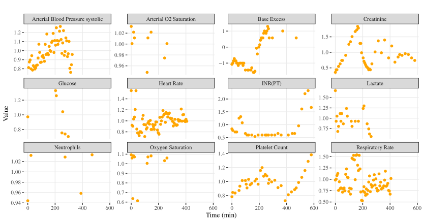
Figure 9: Longitudinal data for 12 clinical features from a patient.

C.3 Imputation for EHR Data

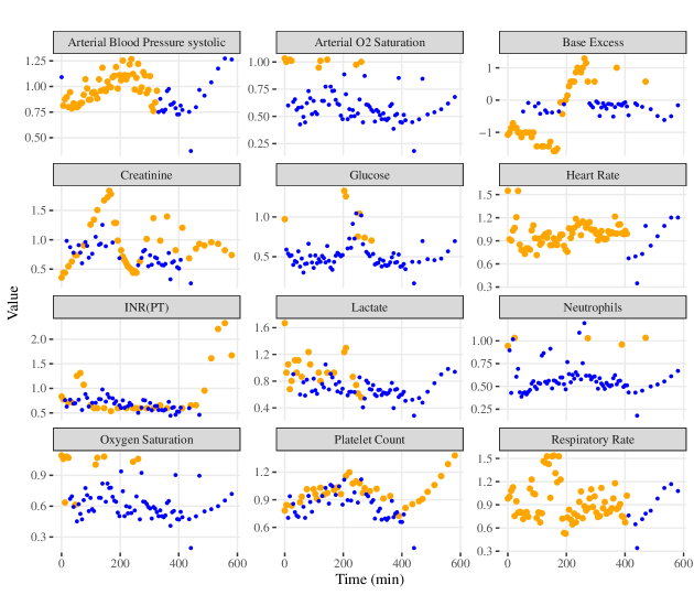
Figure 10: Data imputation by matrix completion on the electronic health record data from a patient.

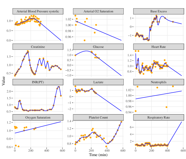
Figure 11: Functional completion by smoothing spline on the electronic health record data from a patient.

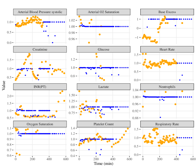
Figure 12: Data imputation by K-NN on the electronic health record data from a patient.

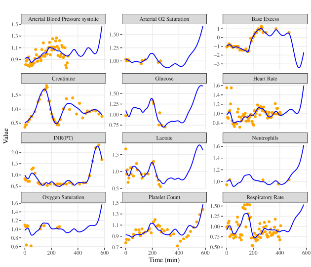
Figure 13: Functional completion by FSVD on the electronic health record data from a patient.

References

• (1)
• Allen and Weylandt (2019) Allen, G. I., and Weylandt, M. (2019), Sparse and functional principal components analysis,, in 2019 IEEE Data Science Workshop (DSW), IEEE, pp. 11–16.
• Aronszajn (1950) Aronszajn, N. (1950), “Theory of reproducing kernels,” Transactions of the American mathematical society, 68(3), 337–404.
• Bai (2003) Bai, J. (2003), “Inferential theory for factor models of large dimensions,” Econometrica, 71(1), 135–171.
• Bai and Ng (2002) Bai, J., and Ng, S. (2002), “Determining the number of factors in approximate factor models,” Econometrica, 70(1), 191–221.
• Baksi et al. (2018) Baksi, K. D., Kuntal, B. K., and Mande, S. S. (2018), “‘TIME’: a web application for obtaining insights into microbial ecology using longitudinal microbiome data,” Frontiers in microbiology, 9, 36.
• Barigozzi et al. (2018) Barigozzi, M., Cho, H., and Fryzlewicz, P. (2018), “Simultaneous multiple change-point and factor analysis for high-dimensional time series,” Journal of Econometrics, 206(1), 187–225.
• Bartlett et al. (2005) Bartlett, P., Bousquet, O., and Mendelson, S. (2005), “Local Rademacher Complexities,” The Annals of Statistics, 33(4), 1497–1537.
• Bertsimas et al. (2018) Bertsimas, D., Pawlowski, C., and Zhuo, Y. D. (2018), “From predictive methods to missing data imputation: an optimization approach,” Journal of Machine Learning Research, 18(196), 1–39.
• Bosq (2000) Bosq, D. (2000), Linear processes in function spaces: theory and applications, Vol. 149 Springer Science & Business Media.
• Bouveyron and Jacques (2011) Bouveyron, C., and Jacques, J. (2011), “Model-based clustering of time series in group-specific functional subspaces,” Advances in Data Analysis and Classification, 5, 281–300.
• Bunea and Xiao (2015) Bunea, F., and Xiao, L. (2015), “On the sample covariance matrix estimator of reduced effective rank population matrices, with applications to fPCA,” Bernoulli, 21(2), 1200–1230.
• Cai and Yuan (2011) Cai, T. T., and Yuan, M. (2011), “Optimal estimation of the mean function based on discretely sampled functional data: Phase transition,” The Annals of Statistics, 39(5), 2330–2355.
• Cai and Zhang (2018) Cai, T. T., and Zhang, A. (2018), “Rate-optimal perturbation bounds for singular subspaces with applications to high-dimensional statistics,” The Annals of Statistics, 46(1), 60–89.
• Candes and Plan (2010) Candes, E. J., and Plan, Y. (2010), “Matrix completion with noise,” Proceedings of the IEEE, 98(6), 925–936.
• Candes and Recht (2012) Candes, E., and Recht, B. (2012), “Exact matrix completion via convex optimization,” Communications of the ACM, 55(6), 111–119.
• Carroll et al. (2020) Carroll, C., Bhattacharjee, S., Chen, Y., Dubey, P., Fan, J., Gajardo, Á., Zhou, X., Müller, H.-G., and Wang, J.-L. (2020), “Time dynamics of COVID-19,” Scientific reports, 10(1), 21040.
• Chen et al. (2017) Chen, K., Delicado, P., and Müller, H.-G. (2017), “Modelling function-valued stochastic processes, with applications to fertility dynamics,” Journal of the Royal Statistical Society Series B: Statistical Methodology, 79(1), 177–196.
• Chen and Lei (2015) Chen, K., and Lei, J. (2015), “Localized functional principal component analysis,” Journal of the American Statistical Association, 110(511), 1266–1275.
• Chiou et al. (2014) Chiou, J.-M., Chen, Y.-T., and Yang, Y.-F. (2014), “Multivariate functional principal component analysis: A normalization approach,” Statistica Sinica, pp. 1571–1596.
• Chiou and Li (2007) Chiou, J.-M., and Li, P.-L. (2007), “Functional clustering and identifying substructures of longitudinal data,” Journal of the Royal Statistical Society Series B: Statistical Methodology, 69(4), 679–699.
• Coffey et al. (2014) Coffey, N., Hinde, J., and Holian, E. (2014), “Clustering longitudinal profiles using P-splines and mixed effects models applied to time-course gene expression data,” Computational Statistics & Data Analysis, 71, 14–29.
• Descary and Panaretos (2019) Descary, M.-H., and Panaretos, V. M. (2019), “Recovering covariance from functional fragments,” Biometrika, 106(1), 145–160.
• Di et al. (2009) Di, C.-Z., Crainiceanu, C. M., Caffo, B. S., and Punjabi, N. M. (2009), “Multilevel functional principal component analysis,” The annals of applied statistics, 3(1), 458.
• Dong et al. (2020) Dong, E., Du, H., and Gardner, L. (2020), “An interactive web-based dashboard to track COVID-19 in real time,” The Lancet infectious diseases, 20(5), 533–534.
• Fan (2018) Fan, J. (2018), Local polynomial modelling and its applications: monographs on statistics and applied probability 66 Routledge.
• Fuentes (2006) Fuentes, M. (2006), “Testing for separability of spatial–temporal covariance functions,” Journal of statistical planning and inference, 136(2), 447–466.
• Giacofci et al. (2013) Giacofci, M., Lambert-Lacroix, S., Marot, G., and Picard, F. (2013), “Wavelet-based clustering for mixed-effects functional models in high dimension,” Biometrics, 69(1), 31–40.
• Golub and Van Loan (1983) Golub, G. H., and Van Loan, C. F. (1983), Matrix Computations John Hopkins University Press.
• Gu (2013) Gu, C. (2013), Smoothing spline ANOVA models, Vol. 297 Springer.
• Hall et al. (2006) Hall, P., Müller, H.-G., and Wang, J.-L. (2006), “Properties of principal component methods for functional and longitudinal data analysis,” The Annals of Statistics, 34(3), 1493–1517.
• Han et al. (2023) Han, R., Shi, P., and Zhang, A. R. (2023), “Guaranteed functional tensor singular value decomposition,” Journal of the American Statistical Association, pp. 1–13.
• Happ and Greven (2018) Happ, C., and Greven, S. (2018), “Multivariate functional principal component analysis for data observed on different (dimensional) domains,” Journal of the American Statistical Association, 113(522), 649–659.
• Hörmann et al. (2015) Hörmann, S., Kidziński, Ł., and Hallin, M. (2015), “Dynamic functional principal components,” Journal of the Royal Statistical Society Series B: Statistical Methodology, 77(2), 319–348.
• Hsing and Eubank (2015) Hsing, T., and Eubank, R. (2015), Theoretical foundations of functional data analysis, with an introduction to linear operators, Vol. 997 John Wiley & Sons.
• Hu and Yao (2022) Hu, X., and Yao, F. (2022), “Sparse functional principal component analysis in high dimensions,” Statistica Sinica, 32(4), 1939–1960.
• Huang et al. (2008) Huang, J. Z., Shen, H., and Buja, A. (2008), “Functional principal components analysis via penalized rank one approximation,” Electronic Journal of Statistics, 2, 678–695.
• Huang et al. (2009) Huang, J. Z., Shen, H., and Buja, A. (2009), “The analysis of two-way functional data using two-way regularized singular value decompositions,” Journal of the American Statistical Association, 104(488), 1609–1620.
• Imaizumi and Kato (2018) Imaizumi, M., and Kato, K. (2018), “PCA-based estimation for functional linear regression with functional responses,” Journal of multivariate analysis, 163, 15–36.
• Jacques and Preda (2013) Jacques, J., and Preda, C. (2013), “Funclust: A curves clustering method using functional random variables density approximation,” Neurocomputing, 112, 164–171.
• Jacques and Preda (2014) Jacques, J., and Preda, C. (2014), “Functional data clustering: a survey,” Advances in Data Analysis and Classification, 8, 231–255.
• James and Sugar (2003) James, G. M., and Sugar, C. A. (2003), “Clustering for sparsely sampled functional data,” Journal of the American Statistical Association, 98(462), 397–408.
• Johnson et al. (2024) Johnson, A., Bulgarelli, L., Pollard, T., Gow, B., Moody, B., Horng, S., Celi, L. A., and Mark, R. (2024), ““MIMIC-IV” (version 3.0),” PhysioNet, .
• Kayano et al. (2010) Kayano, M., Dozono, K., and Konishi, S. (2010), “Functional cluster analysis via orthonormalized Gaussian basis expansions and its application,” Journal of classification, 27, 211–230.
• Kneip and Liebl (2020) Kneip, A., and Liebl, D. (2020), “On the optimal reconstruction of partially observed functional data,” The Annals of Statistics, 48(3), 1692–1717.
• Kodikara et al. (2022) Kodikara, S., Ellul, S., and Lê Cao, K.-A. (2022), “Statistical challenges in longitudinal microbiome data analysis,” Briefings in Bioinformatics, 23(4), bbac273.
• Koner and Staicu (2023) Koner, S., and Staicu, A.-M. (2023), “Second-generation functional data,” Annual review of statistics and its application, 10(1), 547–572.
• Kraus (2015) Kraus, D. (2015), “Components and completion of partially observed functional data,” Journal of the Royal Statistical Society Series B: Statistical Methodology, 77(4), 777–801.
• Lam and Yao (2012) Lam, C., and Yao, Q. (2012), “Factor modeling for high-dimensional time series: inference for the number of factors,” The Annals of Statistics, pp. 694–726.
• Lam et al. (2011) Lam, C., Yao, Q., and Bathia, N. (2011), “Estimation of latent factors for high-dimensional time series,” Biometrika, 98(4), 901–918.
• Li and Xiao (2023) Li, R., and Xiao, L. (2023), “Latent factor model for multivariate functional data,” Biometrics, 79(4), 3307–3318.
• Li et al. (2013) Li, Y., Wang, N., and Carroll, R. J. (2013), “Selecting the number of principal components in functional data,” Journal of the American Statistical Association, 108(504), 1284–1294.
• Liang et al. (2023) Liang, D., Huang, H., Guan, Y., and Yao, F. (2023), “Test of weak separability for spatially stationary functional field,” Journal of the American Statistical Association, 118(543), 1606–1619.
• Luo et al. (2024) Luo, F., Tan, J., Zhang, D., Huang, H., and Shen, Y. (2024), “Functional Clustering for Longitudinal Associations between County-Level Social Determinants of Health and Stroke Mortality in the US,” arXiv preprint arXiv:2406.10499, .
• Lynch and Chen (2018) Lynch, B., and Chen, K. (2018), “A test of weak separability for multi-way functional data, with application to brain connectivity studies,” Biometrika, 105(4), 815–831.
• Martinez et al. (2010) Martinez, J. G., Liang, F., Zhou, L., and Carroll, R. J. (2010), “Longitudinal functional principal component modelling via Stochastic Approximation Monte Carlo,” Canadian Journal of Statistics, 38(2), 256–270.
• Morris (2015) Morris, J. S. (2015), “Functional regression,” Annual Review of Statistics and Its Application, 2(1), 321–359.
• Müller and Yao (2008) Müller, H.-G., and Yao, F. (2008), “Functional additive models,” Journal of the American Statistical Association, 103(484), 1534–1544.
• Ng et al. (2001) Ng, A., Jordan, M., and Weiss, Y. (2001), “On spectral clustering: Analysis and an algorithm,” Advances in neural information processing systems, 14.
• Nie et al. (2022) Nie, Y., Yang, Y., Wang, L., and Cao, J. (2022), “Recovering the underlying trajectory from sparse and irregular longitudinal data,” Canadian Journal of Statistics, 50(1), 122–141.
• Pan and Yao (2008) Pan, J., and Yao, Q. (2008), “Modelling multiple time series via common factors,” Biometrika, 95(2), 365–379.
• Panaretos and Tavakoli (2013) Panaretos, V. M., and Tavakoli, S. (2013), “Cramér–Karhunen–Loève representation and harmonic principal component analysis of functional time series,” Stochastic Processes and their Applications, 123(7), 2779–2807.
• Peng and Müller (2008) Peng, J., and Müller, H.-G. (2008), “Distance-based clustering of sparsely observed stochastic processes, with applications to online auctions,” The Annals of applied statistics, 2(3), 1056–1077.
• Qiao et al. (2019) Qiao, X., Guo, S., and James, G. M. (2019), “Functional graphical models,” Journal of the American Statistical Association, 114(525), 211–222.
• Ramsay and Silvermann (2005) Ramsay, J., and Silvermann, B. (2005), Functional data analysis. springer series in statistics Wiley Online Library.
• Rand (1971) Rand, W. M. (1971), “Objective criteria for the evaluation of clustering methods,” Journal of the American Statistical association, 66(336), 846–850.
• Reiss et al. (2017) Reiss, P. T., Goldsmith, J., Shang, H. L., and Ogden, R. T. (2017), “Methods for scalar-on-function regression,” International Statistical Review, 85(2), 228–249.
• Ross et al. (2014) Ross, M., Wei, W., and Ohno-Machado, L. (2014), ““Big data” and the electronic health record,” Yearbook of medical informatics, 23(01), 97–104.
• Scheipl et al. (2015) Scheipl, F., Staicu, A.-M., and Greven, S. (2015), “Functional additive mixed models,” Journal of Computational and Graphical Statistics, 24(2), 477–501.
• Scheurwegs et al. (2017) Scheurwegs, E., Cule, B., Luyckx, K., Luyten, L., and Daelemans, W. (2017), “Selecting relevant features from the electronic health record for clinical code prediction,” Journal of biomedical informatics, 74, 92–103.
• Schölkopf et al. (2001) Schölkopf, B., Herbrich, R., and Smola, A. J. (2001), A generalized representer theorem,, in International conference on computational learning theory, Springer, pp. 416–426.
• Serban and Wasserman (2005) Serban, N., and Wasserman, L. (2005), “CATS: clustering after transformation and smoothing,” Journal of the American Statistical Association, 100(471), 990–999.
• Shen and Huang (2008) Shen, H., and Huang, J. Z. (2008), “Sparse principal component analysis via regularized low rank matrix approximation,” Journal of multivariate analysis, 99(6), 1015–1034.
• Shi et al. (2023) Shi, P., Martino, C., Han, R., Janssen, S., Buck, G., Serrano, M., Owzar, K., Knight, R., Shenhav, L., and Zhang, A. R. (2023), “Time-Informed Dimensionality Reduction for Longitudinal Microbiome Studies,” bioRxiv, pp. 2023–07.
• Shou et al. (2015) Shou, H., Zipunnikov, V., Crainiceanu, C. M., and Greven, S. (2015), “Structured functional principal component analysis,” Biometrics, 71(1), 247–257.
• Speckman (1985) Speckman, P. (1985), “Spline smoothing and optimal rates of convergence in nonparametric regression models,” The Annals of Statistics, pp. 970–983.
• Stekhoven and Bühlmann (2012) Stekhoven, D. J., and Bühlmann, P. (2012), “MissForest—non-parametric missing value imputation for mixed-type data,” Bioinformatics, 28(1), 112–118.
• Stone (1982) Stone, C. J. (1982), “Optimal global rates of convergence for nonparametric regression,” The annals of statistics, pp. 1040–1053.
• Tan et al. (2022) Tan, J., Ge, Y., Martinez, L., Sun, J., Li, C., Westbrook, A., Chen, E., Pan, J., Li, Y., Cheng, W. et al. (2022), “Transmission roles of symptomatic and asymptomatic COVID-19 cases: a modelling study,” Epidemiology & Infection, 150, e171.
• Tan et al. (2024) Tan, J., Liang, D., Guan, Y., and Huang, H. (2024), “Graphical principal component analysis of multivariate functional time series,” Journal of the American Statistical Association, pp. 1–24.
• Tian et al. (2021) Tian, T., Tan, J., Luo, W., Jiang, Y., Chen, M., Yang, S., Wen, C., Pan, W., and Wang, X. (2021), “The effects of stringent and mild interventions for coronavirus pandemic,” Journal of the American Statistical Association, 116(534), 481–491.
• Tsybakov (2009) Tsybakov, A. B. (2009), “Introcuction to Nonparametric Estimation,” Introduction to Nonparametric Estimation, pp. 1–76.
• Vershynin (2018) Vershynin, R. (2018), High-dimensional probability: An introduction with applications in data science, Vol. 47 Cambridge university press.
• Wang et al. (2016) Wang, J.-L., Chiou, J.-M., and Müller, H.-G. (2016), “Functional data analysis,” Annual Review of Statistics and its application, 3, 257–295.
• Witten et al. (2009) Witten, D. M., Tibshirani, R., and Hastie, T. (2009), “A penalized matrix decomposition, with applications to sparse principal components and canonical correlation analysis,” Biostatistics, 10(3), 515–534.
• Yang et al. (2011) Yang, W., Müller, H.-G., and Stadtmüller, U. (2011), “Functional singular component analysis,” Journal of the Royal Statistical Society Series B: Statistical Methodology, 73(3), 303–324.
• Yao and Lee (2006) Yao, F., and Lee, T. C. (2006), “Penalized spline models for functional principal component analysis,” Journal of the Royal Statistical Society Series B: Statistical Methodology, 68(1), 3–25.
• Yao et al. (2005a) Yao, F., Müller, H.-G., and Wang, J.-L. (2005a), “Functional data analysis for sparse longitudinal data,” Journal of the American statistical association, 100(470), 577–590.
• Yao et al. (2005b) Yao, F., Müller, H.-G., and Wang, J.-L. (2005b), “Functional linear regression analysis for longitudinal data,” Ann. Statist., 33(1), 2873–2903.
• Yu et al. (2016) Yu, H.-F., Rao, N., and Dhillon, I. S. (2016), “Temporal regularized matrix factorization for high-dimensional time series prediction,” Advances in neural information processing systems, 29.
• Yuan and Cai (2010) Yuan, M., and Cai, T. T. (2010), “A reproducing kernel Hilbert space approach to functional linear regression,” The Annals of Statistics, 38(6), 3412–3444.
• Zapata et al. (2022) Zapata, J., Oh, S.-Y., and Petersen, A. (2022), “Partial separability and functional graphical models for multivariate Gaussian processes,” Biometrika, 109(3), 665–681.
• Zhang and Chen (2022) Zhang, A. R., and Chen, K. (2022), “Nonparametric covariance estimation for mixed longitudinal studies, with applications in midlife women’s health,” Statistica Sinica, 32(1), 345–365.
• Zhang, Pan, Yao and Zhou (2024) Zhang, B., Pan, G., Yao, Q., and Zhou, W. (2024), “Factor modeling for clustering high-dimensional time series,” Journal of the American Statistical Association, 119(546), 1252–1263.
• Zhang, Xue, Xu, Lee and Qu (2024) Zhang, J., Xue, F., Xu, Q., Lee, J., and Qu, A. (2024), “Individualized dynamic latent factor model for multi-resolutional data with application to mobile health,” Biometrika, p. asae015.
• Zhang et al. (2013) Zhang, L., Shen, H., and Huang, J. Z. (2013), “Robust regularized singular value decomposition with application to mortality data,” The Annals of Applied Statistics, pp. 1540–1561.