Time-Reversal Symmetry in RDMFT and pCCD with Complex-Valued Orbitals

Abstract

Reduced density matrix functional theory (RDMFT) and coupled cluster theory restricted to paired double excitations (pCCD) are emerging as efficient methodologies for accounting for the so-called non-dynamic electronic correlation effects. Up to now, molecular calculations have been performed with real-valued orbitals. However, before extending the applicability of these methodologies to extended systems, where Bloch states are employed, the subtleties of working with complex-valued orbitals and the consequences of imposing time-reversal symmetry must be carefully addressed. In this work, we describe the theoretical and practical implications of adopting time-reversal symmetry in RDMFT and pCCD when allowing for complex-valued orbital coefficients. The theoretical considerations primarily affect the optimization algorithms, while the practical implications raise fundamental questions about the stability of solutions. Specifically, we find that complex solutions lower the energy when non-dynamic electronic correlation effects are pronounced. We present numerical examples to illustrate and discuss these instabilities and possible problems introduced by $N$-representability violations.

I Introduction

In quantum chemistry, accurately describing the so-called electronic correlation effectsLöwdin (1955) remains an open problem. For practical purposes, it has been convenient to classify these effects as dynamic and non-dynamic, where the former can be interpreted as small corrections on top of the Hartree-Fock (HF) reference determinant and the latter refers to major changes in the electronic wave function caused by (near-)degeneracies in the single-particle states. Cioslowski (1991) Accounting for the so-called non-dynamic electronic correlation effects in quantum chemistry has been routinely tackled using multiconfigurational self-consistent field methodologies, Helgaker, Jorgensen, and Olsen (2000); Malmqvist and Roos (1989) such as complete-active-space self-consistent field (CASSCF),Roos, Taylor, and Sigbahn (1980); Roos (1980, 2005) complete-active-space configuration interaction (CASCI), or density-matrix renormalization group (DMRG). White (1992, 1993); Chan and Sharma (2011); Baiardi and Reiher (2020) However, their applicability is limited due to the exponential growth of their computational cost with respect to the system size.

Alternative methodologies like reduced density matrix functional theory Gilbert (1975); Valone (1991) (RDMFT) and coupled-cluster theory restricted to paired double excitations Henderson et al. (2014) (pCCD) are recently gaining practitioners in the electronic structure community. Piris (2013a, 2018, 2021); Mitxelena and Piris (2020a, b, 2024); Rodríguez-Mayorga, Giesbertz, and Visscher (2022); Henderson et al. (2014); Boguslawski et al. (2012); Boguslawski (2021); Nowak, Legeza, and Boguslawski (2021); Gałynśka and Boguslawski (2024); Kossoski and Loos (2023); Kossoski et al. (2021); Ravi et al. (2023); Marie, Kossoski, and Loos (2021) Within these methodologies, diagonalization of large matrices is replaced by the optimization of occupation numbers or amplitudes, which reduces drastically the computational cost. Furthermore, these methodologies are cost-effective approaches to deal with the so-called non-dynamic electronic correlation effects Piris (2013a); Mitxelena and Piris (2020a, b); Henderson et al. (2014); Boguslawski et al. (2012); Gałynśka and Boguslawski (2024) because the optimization procedure introduces fractional occupation numbers that adjust to the degeneracies present in the system under investigation. For this reason, the most simple RDMFT approximations, the Müller Muller and Willner (1993) and power Sharma et al. (2008); Cioslowski and Pernal (2000) functionals, have already been employed to study strongly correlated materials such as nickel oxides, Sharma et al. (2008, 2013) where these methods describe precisely the characteristic Mott-insulator nature of these materials. The success of pCCD can be attributed to its connection with seniority-zero methods, particularly perfect pairing and generalized valence bond approaches. Cullen (1996); Stein, Henderson, and Scuseria (2014); Kutzelnigg (2012); Voorhis and Head-Gordon (2000); Van Voorhis and Head-Gordon (2001); Small and Head-Gordon (2012) However, to achieve quantitatively meaningful results, pCCD must be combined with an orbital optimization procedure. Henderson et al. (2014)

It is known that the usual operators employed in quantum chemistry are real-valued in time-independent applications. Hence, the use of complex orbitals has been less explored in favor of real orbitals. Nevertheless, complex orbitals have attracted attention from the community due to the extra flexibility provided by the complex parameterization. Fukutome (1981); Scuseria et al. (2011); Jiménez-Hoyos et al. (2012); Small, Sundstrom, and Head-Gordon (2015); Jiménez-Hoyos, Henderson, and Scuseria (2011); Song, Henderson, and Scuseria (2004); Stuber and Paldus (2003) Specifically, it has shown to be an efficient alternative to multiconfigurational methods to account for non-dynamic electronic correlation effects with single-determinant wave functions.Jiménez-Hoyos, Henderson, and Scuseria (2011); Song, Henderson, and Scuseria (2004); Stuber and Paldus (2003) However, complex-valued orbitals must be used carefully because they break symmetries among the spin-up ($\uparrow$) and spin-down ($\downarrow$) electrons trivially granted by real-valued orbitals.

In the absence of spin-orbit coupling contributions to the Hamiltonian or external magnetic fields, the spin-with orbitals ($\chi_{p\uparrow}$ and $\chi_{p\downarrow}$) are typically constructed as the direct product between a spin function ($\uparrow$ or $\downarrow$) and a spatial function $\chi_{p}({\boldsymbol{r}})=\sum_{\mu}c_{\mu p}\psi_{\mu}({\boldsymbol{r}})$ built as a linear combination of real atomic orbitals $\psi_{\mu}(\boldsymbol{r})$, where the matrix $\boldsymbol{c}$ gathers the molecular orbital coefficients. In general, real orbitals ($\boldsymbol{c}\in\mathbb{R}$) are constructed to preserve fundamental symmetries such as spin symmetries ($\hat{S}_{z}$ and $\hat{S}^{2}$), complex conjugation ($\hat{\mathcal{K}}$), and time-reversal symmetry ($\hat{\Theta}$). On the contrary, working with complex orbitals ($\boldsymbol{c}\in\mathbb{C}$), one is forced to preserve either $\hat{S}^{2}$ and $\hat{S}_{z}$ (charge current wave in Fukutome’s classification) or $\hat{\Theta}$ and $\hat{S}_{z}$ (axial spin current wave in Fukutome’s classification). Fukutome (1981); Stuber and Paldus (2003); Jiménez-Hoyos, Henderson, and Scuseria (2011); Small, Sundstrom, and Head-Gordon (2015) In the former case, the spatial part of the orbitals, $\chi_{p}(\boldsymbol{r})$, for the spin-up and spin-down electrons is identical, which guarantees the correct value of $\expectationvalue*{\hat{S}^{2}}$. In the latter case, the spin-up orbitals, $\chi_{p\uparrow}(\boldsymbol{r})$, are related to the spin-down orbitals, $\chi_{p\downarrow}(\boldsymbol{r})$, as

$$\begin{split}\hat{\Theta}\chi_{p\uparrow}(\boldsymbol{r})&=\hat{\Theta}\chi_{p}(\boldsymbol{r})\matrixquantity(1\\ 0)=-\mathrm{i}\;\sigma_{y}\;\hat{\mathcal{K}}\chi_{p}(\boldsymbol{r})\matrixquantity(1\\ 0)\\ &=-\mathrm{i}\matrixquantity(0\hfil&-\mathrm{i}\\ \mathrm{i}&0)\hat{\mathcal{K}}\chi_{p}(\boldsymbol{r})\matrixquantity(1\\ 0)=\chi^{*}_{p}(\boldsymbol{r})\matrixquantity(0\\ 1)=\chi_{p\downarrow}(\boldsymbol{r}),\end{split}$$ (1)

where $\mathrm{i}=\sqrt{-1}$ and $\sigma_{y}$ is a Pauli matrix. This option preserves time-reversal symmetry, that is, $\hat{\Theta}\chi_{p\uparrow}(\boldsymbol{r})=\chi_{p\downarrow}(\boldsymbol{r})$ and $\hat{\Theta}\chi_{p\downarrow}(\boldsymbol{r})=-\chi_{p\uparrow}(\boldsymbol{r})$, but not $\hat{S}^{2}$.

Before proceeding further, let us express the spin-with orbitals obtained by imposing time-reversal symmetry in matrix form as

$$\begin{split}{\boldsymbol{\chi}}_{\sigma}=\boldsymbol{C}\cdot{\boldsymbol{\psi}}=\matrixquantity(\boldsymbol{c}&{\bf 0}\\ {\bf 0}&\boldsymbol{c}^{*})\cdot{\boldsymbol{\psi}},\end{split}$$ (2)

where ${\boldsymbol{\chi}}_{\sigma}$ represents all the spin-with orbitals organized in a single column, and ${\boldsymbol{\psi}}=\{\matrixquantity(\psi\\ 0),\matrixquantity(0\\ \psi)\}$ contains the spin-with atomic orbitals, ordered such that all spin-up orbitals are listed first. As previously mentioned, this convention also preserves $\hat{S}_{z}$ (i.e., it fixes the number of spin-up and spin-down electrons). However, the axis chosen for the quantization is irrelevant for Hamiltonians that do not account for spin-orbit coupling effects or external magnetic fields. Therefore, we equally well may have chosen to preserve $\hat{S}_{y}$ whose eigenstates ($\chi^{y}_{p\uparrow}$ and $\chi^{y}_{p\downarrow}$) are given as a linear combination of their spin-up and spin-down counterparts quantized with respect to the $z$ axis, i.e.,

$$\chi^{y}_{p\uparrow}(\boldsymbol{r}) =\frac{\chi_{p\uparrow}({\boldsymbol{r}})+\mathrm{i}\chi_{p\downarrow}({\boldsymbol{r}})}{\sqrt{2}}, \chi^{y}_{p\downarrow}(\boldsymbol{r}) =\frac{\mathrm{i}\chi_{p\uparrow}({\boldsymbol{r}})+\chi_{p\downarrow}({\boldsymbol{r}})}{\sqrt{2}},$$ (3)

which also preserves time-reversal symmetry. Next, let us write the corresponding eigenstates in matrix form as

$$\begin{split}{\boldsymbol{\chi}}_{\sigma}^{y}=\frac{1}{\sqrt{2}}\boldsymbol{C}^{y}\cdot{\boldsymbol{\psi}}=\frac{1}{\sqrt{2}}\matrixquantity(\boldsymbol{c}&\mathrm{i}\boldsymbol{c}^{*}\\ \mathrm{i}\boldsymbol{c}&\boldsymbol{c}^{*})\cdot{\boldsymbol{\psi}}=\matrixquantity(\real(\boldsymbol{c})&\imaginary(\boldsymbol{c})\\ -\imaginary(\boldsymbol{c})&\real(\boldsymbol{c}))\cdot{\boldsymbol{\psi}},\end{split}$$ (4)

where we have summed the coefficients ($\boldsymbol{C}^{y}$) with their complex conjugate to obtain the final form. Note that this selection leads to pure real coefficients at the expense of introducing 2-component spinors, which shows that working with complex orbitals that preserve time-reversal symmetry is equivalent to using 2-component real spinors that also preserve time-reversal symmetry. In particular, when applied to the HF approximation, the latter corresponds to the real-paired generalized HF method.This option is not included in Ref. Jiménez-Hoyos, Henderson, and Scuseria, 2011, where real coefficients are employed, time-reversal symmetry is preserved, but not $\hat{S}^{2}$.

In this work, we have preferred to work with complex orbitals (instead of 2-component real spinors) and preserve $\hat{S}_{z}$. Also, we have enforced the spin-up and spin-down orbitals to be related by complex conjugation of the spatial part to preserve time-reversal symmetry. Thus, deviations from the physical $\expectationvalue*{\hat{S}^{2}}$ value (i.e., spin contamination) might occur. This selection is motivated by three reasons: (i) time-reversal symmetry is typically imposed in codes that can deal with complex orbitals/one-body states for extended systems (e.g. ABINIT Gonze et al. (2020) or QUANTUM ESPRESSO, Giannozzi et al. (2009, 2017) see also Appendix B in Ref. Denawi et al., 2023), (ii) the simplification in the RDMFT and pCCD equations facilitates their extension to complex-valued orbitals, and (iii) it corresponds to the correct non-relativistic limit when time-reversal symmetry is employed to build the 4-component spinors that are employed in the solution of the Dirac-Coulomb/Coulomb-Gaunt Hamiltonians. Dyall and Fægri Jr (2007)

To gain further insights into this limit, let us first mention that the relativistic 4-component spinors are complex-valued and can be chosen to preserve time-reversal symmetry in the absence of external magnetic fields (i.e., forming Kramers’ pairs Kramers (1930); Aucar, Jensen, and Oddershede (1995); Bučinskỳ et al. (2015); Bučinskỳ, Malček, and Biskupič (2016); Komorovsky, Repisky, and Bučinskỳ (2016)). They are usually expanded in two distinct basis sets, one for the upper (large) components and one for the lower (small) components of the Dirac wave function. For better comparison with non-relativistic basis set expansions, it is therefore convenient to perform an exact transformation to the 2-spinor (X2C) form. Jensen ; Kutzelnigg and Liu (2005); Iliaš and Saue (2007) The expansion coefficients for these X2C-spinors are complex and the preservation of time-reversal symmetry is easily visible when they are written in matrix form as

$$\begin{split}\matrixquantity(\boldsymbol{c}_{L\uparrow}&\boldsymbol{c}_{L\downarrow}\\ -\boldsymbol{c}_{L\downarrow}^{*}&\boldsymbol{c}_{L\uparrow}^{*}).\end{split}$$ (5)

This corresponds to the torsional spin current wave (TSCW) in Fukutome’s classification. Fukutome (1981); Jiménez-Hoyos, Henderson, and Scuseria (2011) In the X2C form, it is possible to use the Dirac identity to remove spin-orbit coupling terms from the Hamiltonian. This simplifies the matrix representation of the Hamiltonian, making it real-symmetric, and thus, one typically proceeds using real coefficients, as seen in Eq. 4. It is important to note that taking either real 2-spinors or (equivalently, as discussed before) complex orbitals, corresponds to a reduction of the variational freedom that complex 2-spinors possess compared to real spatial orbitals. Despite this, both choices still retain more freedom than real spatial orbitals. Real spatial orbitals are thus only obtained during orbital optimization if the additional freedom provided by the complex coefficients does not lead to a lower energy solution according to the variational principle (see Sec. IV.3).

Here, we examine the role of complex orbitals in extending the applicability of the most recently developed RDMFT functionals and pCCD to systems described by complex single-particle states. In Sec. II, we briefly introduce RDMFT (Sec. II.1), pCCD (Sec. II.2), and the orbital optimization procedure proposed by Ugalde and Piris (Sec. II.3), Piris and Ugalde (2009) which is currently applied in most RDMFT calculations. Then, in Sec. III, we discuss the effect of time-reversal symmetry on the RDMFT and pCCD energy expressions and its impact on the orbital optimization procedure. Finally, in Sec. IV, we present some numerical examples that illustrate the consequences of using complex-valued orbital coefficients and time-reversal symmetry in practical calculations for spin-compensated systems. Our conclusions are drawn in Sec. V. Unless otherwise stated, atomic units are used throughout.

II Theoretical background

II.1 Reduced Density Matrix Functional Theory

In 1975, Gilbert Gilbert (1975) proposed an extension of the Hohenberg-Kohn theorem Hohenberg and Kohn (1964) for non-local external potentials, which introduces the energy as a functional of the first-order reduced density matrix (1RDM) $\gamma$. It generalizes the functional based on the electronic density $\rho$ that is employed in density-functional theory.Burke and friends (2007) A compact representation of $\gamma$ is obtained by expressing it in the natural orbital basis

$$\gamma(\boldsymbol{r},\boldsymbol{r}^{\prime})=\sum_{p}\sum_{\sigma=\uparrow,\downarrow}n_{p\sigma}\chi_{p\sigma}^{*}(\boldsymbol{r})\chi_{p\sigma}(\boldsymbol{r}^{\prime}),$$ (6)

where $n_{p\sigma}\in\quantity[0,1]$ is the occupation number associated with the natural spin-orbital $\chi_{p\sigma}$. For $\boldsymbol{r}=\boldsymbol{r}^{\prime}$, it reduces to the electron density, that is, $\rho(\boldsymbol{r})=\gamma(\boldsymbol{r},\boldsymbol{r})$. In practical realizations of RDMFT, the matrix elements of the second-order reduced density matrix (2RDM) ${}^{2}D^{\sigma\sigma^{\prime}}_{pq,rs}=\matrixelement{\Psi}{{\hat{c}^{\dagger}}_{p\sigma}{\hat{c}^{\dagger}}_{q\sigma^{\prime}}{\hat{c}^{\vphantom{\dagger}}}_{s\sigma^{\prime}}{\hat{c}^{\vphantom{\dagger}}}_{r\sigma}}{\Psi}$ (with $\sigma^{\prime}=\ \uparrow$ or $\downarrow$) are expressed as functions of the occupation numbers and the natural orbitals are employed to compute the two-electron repulsion integrals. Here, ${\hat{c}^{\dagger}}_{p\sigma}$ (${\hat{c}^{\vphantom{\dagger}}}_{p\sigma}$) is the usual creation (annihilation) operator and $\Psi$ is the exact $N$-electron wave function. In the most basic RDMFT approximations, the 2RDM elements of the opposite-spin ($\sigma\neq\sigma^{\prime}$) and same-spin ($\sigma=\sigma^{\prime}$) blocks read

$${}^{2}D^{\sigma\sigma^{\prime}}_{pq,rs} =\frac{n_{p\sigma}n_{q\sigma^{\prime}}}{2}\delta_{pr}\delta_{qs},$$ (7a)

$${}^{2}D^{\sigma\sigma}_{pq,rs} =\frac{n_{p\sigma}n_{q\sigma}}{2}\delta_{pr}\delta_{qs}-\frac{f(n_{p\sigma},n_{q\sigma})}{2}\delta_{ps}\delta_{qr},$$ (7b)

with $f(n_{p\sigma},n_{q\sigma})$ being a simple function of the occupations numbers. For example, $f(n_{p\sigma},n_{q\sigma})=\sqrt{n_{p\sigma}n_{q\sigma}}$ in the Müller functional Müller (1984); Buijse and Baerends (2002); Buijse (1991) and $f(n_{p\sigma},n_{q\sigma})=(n_{p\sigma}n_{q\sigma})^{\alpha}$ with $\alpha\in\mathbb{R}^{+}$ in the power functional Sharma et al. (2008); Cioslowski and Pernal (2000). Note that the elements ${}^{2}D^{\sigma\sigma^{\prime}}_{pq,pq}=n_{p\sigma}n_{q\sigma}/2$ correspond to Hartree contributions while the terms ${}^{2}D^{\sigma\sigma}_{pq,qp}=-f(n_{p\sigma},n_{q\sigma})/2$ are modified exchange contributions that account for electronic correlation effects. Hence, these approximations are $JK$-only functionals Rodríguez-Mayorga et al. (2017) because only Hartree ($J$) and exchange ($K$) integrals are required in the evaluation of the electronic energy. However, more advanced RDMFT functionals based on the reconstruction of the second-order cumulant matrix, such as PNOF$i$ Piris (2013a, b, 2017) ($i=5$, $6$, and $7$) and GNOF, Piris (2021) include the additional $L$ integrals Piris (1999), defined below. Thus, they are usually referred to as $JKL$-only approximations. For spin-compensated systems ($n_{p}=n_{p\uparrow}=n_{p\downarrow}$), the electronic energy functional of PNOF$i$ and GNOF takes the following form

$$E^{\text{RDMFT}}=2\sum_{p}n_{p}h_{pp}+\sum_{pq}\quantity({}^{2}D_{pq,pq}J_{pq}+{}^{2}D_{pq,qp}K_{pq}+{}^{2}D_{pp,qq}L_{pq}),$$ (8)

where the one-electron integrals are

$$h_{pq}=\int\differential\boldsymbol{r}\chi^{*}_{p}(\boldsymbol{r})\hat{h}\chi_{q}(\boldsymbol{r}),$$ (9)

with $\hat{h}=-\nabla^{2}_{\boldsymbol{r}}/2+v_{\text{ext}}(\boldsymbol{r})$ being the (one-electron) core Hamiltonian and $v_{\text{ext}}(\boldsymbol{r})$ is the external potential. The various types of two-electron integrals

$$J_{pq} =\innerproduct{pq}{pq}, K_{pq} =\innerproduct{pq}{qp}, L_{pq} =\innerproduct{pp}{qq},$$ (10)

are expressed in terms of the spatial part of the natural orbital basis,

$$\innerproduct{pq}{rs}=\iint\differential\boldsymbol{r}\differential\boldsymbol{r}^{\prime}\frac{\chi_{p}^{*}(\boldsymbol{r})\chi_{q}^{*}(\boldsymbol{r}^{\prime})\chi_{r}(\boldsymbol{r})\chi_{s}(\boldsymbol{r}^{\prime})}{\absolutevalue{\boldsymbol{r}-\boldsymbol{r}^{\prime}}}.$$ (11)

Note that, here, we have employed the spin-summed 2RDM elements, i.e., ${}^{2}D_{pq,rs}=\sum_{\sigma\sigma^{\prime}}{}^{2}D^{\sigma\sigma^{\prime}}_{pq,rs}$. It is worth mentioning that Löwdin normalization is used throughout this work, that is, $\Tr\quantity[{}^{2}{\boldsymbol{D}}]=N(N-1)/2$ with $N$ being the number of electrons.

The energy contribution involving $L$ integrals arises from the interaction of opposite-spin electrons, i.e.

$$\sum_{pq}{}^{2}D_{pp,qq}L_{pq}=\sum_{pq}\sum_{\sigma\neq\sigma^{\prime}}{}^{2}D^{\sigma\sigma^{\prime}}_{pp,qq}L_{pq},$$ (12)

because the same-spin contributions cancel due to the Pauli exclusion principle (i.e., ${}^{2}D^{\sigma\sigma}_{pp,qq}=0$). For real orbitals, it is easy to verify that $L_{pq}=K_{pq}$. Thus, the last term in Eq. 8 is usually combined with the second term and the electronic energy is written using only $J$ and $K$ integrals. However, the $K$ and $L$ integrals differ for complex orbitals unless one imposes time-reversal symmetry (see below). It is easy to show that $J$ and $K$ integrals are real even for complex orbitals. On the contrary, $L$ integrals are complex-valued in general.

II.2 Coupled Cluster With Paired Doubles

The pCCD approximation belongs to the coupled-cluster (CC) family of methods, which aims to go beyond the single-determinant wave function $\ket{0}$ to describe the many-body state using the wave operator $e^{\hat{T}}$ to produce excited determinants from the reference determinant. In pCCD, for spin-compensated systems, the many-body wave function is expressed as $\ket{\Psi}=e^{\hat{T}}\ket{0}$, where the excitation operator is restricted to paired double excitations Henderson et al. (2014)

$$\hat{T}=\sum_{i}^{N/2}\sum_{a=N/2+1}^{M}t_{i}^{a}{\hat{c}^{\dagger}}_{a\uparrow}{\hat{c}^{\dagger}}_{a\downarrow}{\hat{c}^{\vphantom{\dagger}}}_{i\downarrow}{\hat{c}^{\vphantom{\dagger}}}_{i\uparrow},$$ (13)

where $M$ is the total number of spatial orbitals and the $t_{i}^{a}$’s are the so-called amplitudes that are optimized by solving the so-called amplitude (or residual) equations

$$\begin{split}0&=\matrixelement{0}{{\hat{c}^{\dagger}}_{i\uparrow}{\hat{c}^{\dagger}}_{i\downarrow}{\hat{c}^{\vphantom{\dagger}}}_{a\downarrow}{\hat{c}^{\vphantom{\dagger}}}_{a\uparrow}\bar{H}}{0}\\ &=L_{ai}+2\quantity(f_{a}^{a}-f_{i}^{i}-\sum_{j}L_{ja}t_{j}^{a}-\sum_{b}L_{ib}t_{i}^{b})t_{i}^{a}\\ &-2\quantity(2J_{ia}-K_{ia}-L_{ia}t_{i}^{a})t_{i}^{a}+\sum_{b}L_{ba}t_{i}^{b}+\sum_{j}L_{ji}t_{j}^{a}+\sum_{jb}L_{jb}t_{j}^{a}t_{i}^{b},\end{split}$$ (14)

where $\bar{H}=e^{-\hat{T}}\hat{H}e^{\hat{T}}$ is the similarity-transformed Hamiltonian, $f_{p}^{q}$ are the Fock matrix elements evaluated with $\ket{0}$, and $i$ and $j$ ($a$ and $b$) refer to occupied (virtual) orbitals with respect to $\ket{0}$. The amplitude equations, which are quadratic in $t$, can be solved in $M^{3}$ computational cost by building the intermediate $y_{i}^{j}=\sum_{b}L_{jb}t_{i}^{b}$.

Let us introduce the pCCD energy functional as

$$E^{\text{pCCD}}=\matrixelement{\mathcal{L}}{\bar{H}}{0},$$ (15)

where $\bra{\mathcal{L}}=\bra{0}(1+\hat{Z})$ is the left eigenvector of $\bar{H}$ and $\hat{Z}=\sum_{ia}z_{i}^{a}{\hat{c}^{\dagger}}_{i\uparrow}{\hat{c}^{\dagger}}_{i\downarrow}{\hat{c}^{\vphantom{\dagger}}}_{a\downarrow}{\hat{c}^{\vphantom{\dagger}}}_{a\uparrow}$ is a deexcitation operator. The stationary conditions $\partialderivative*{E^{\text{pCCD}}}{z_{i}^{a}}=0$ yield the $t$-amplitude equations [see Eq. 14] while the additional conditions $\partialderivative*{E^{\text{pCCD}}}{t_{i}^{a}}=0$ allows us to write the (linear) residual equations for the left amplitudes $\{z_{i}^{a}\}$ as

$$\begin{split}0&=L_{ia}+2\quantity(f_{a}^{a}-f_{i}^{i}-\sum_{j}L_{ja}t_{j}^{a}-\sum_{b}L_{ib}t_{i}^{b})z_{i}^{a}-2\quantity(2J_{ia}-K_{ia}-2L_{ia}t_{i}^{a})z_{i}^{a}\\ &+\sum_{b}L_{ab}z_{i}^{b}+\sum_{j}L_{ij}z_{j}^{a}+\sum_{jb}t_{j}^{b}\left(L_{ib}z_{j}^{a}+L_{ja}z_{i}^{b}\right)-2L_{ia}\quantity(\sum_{j}z_{j}^{a}t_{j}^{a}+\sum_{b}z_{i}^{b}t_{i}^{b}).\end{split}$$ (16)

Next, with the aid of the $t$- and $z$-amplitude equations, one can easily compute the 1RDM, which is diagonal within the pCCD approximation Henderson et al. (2014)

$${}^{1}D^{\sigma}_{p,q}=\matrixelement{0}{(1+\hat{Z})e^{-\hat{T}}{\hat{c}^{\dagger}}_{p\sigma}{\hat{c}^{\vphantom{\dagger}}}_{q\sigma}e^{\hat{T}}}{0}\delta_{pq}=n_{p\sigma}\delta_{pq},$$ (17)

and directly linked to the occupation numbers that can be written as $n_{i\sigma}=(1-x_{i}^{i})$ and $n_{a\sigma}=x_{a}^{a}$ with $x_{i}^{j}=\sum_{a}t_{i}^{a}z_{j}^{a}$ and $x_{a}^{b}=\sum_{i}t_{i}^{b}z_{i}^{a}$. Similarly, we may write the matrix elements of the spin-summed 2RDM

$${}^{2}D_{pq,rs}=\sum_{\sigma\sigma^{\prime}}\matrixelement{0}{(1+\hat{Z})e^{-\hat{T}}{\hat{c}^{\dagger}}_{p\sigma}{\hat{c}^{\dagger}}_{q\sigma^{\prime}}{\hat{c}^{\vphantom{\dagger}}}_{s\sigma^{\prime}}{\hat{c}^{\vphantom{\dagger}}}_{r\sigma}e^{\hat{T}}}{0},$$ (18)

as

$${}^{2}D_{ii,jj} =x_{i}^{j}+\delta_{ij}(1-2x_{i}^{i}),$$ (19a)

$${}^{2}D_{ii,aa} =t_{i}^{a}+x_{i}^{a}-2t_{i}^{a}(x_{a}^{a}+x_{i}^{i}-t_{i}^{a}z_{i}^{a}),$$ (19b)

$${}^{2}D_{aa,ii} =z_{i}^{a},$$ (19c)

$${}^{2}D_{aa,bb} =x_{a}^{b},$$ (19d)

$${}^{2}D_{ij,ij} =2(1-x_{i}^{i}x_{j}^{j})+\delta_{ij}3(x_{i}^{i}-1),$$ (19e)

$${}^{2}D_{ia,ia} ={}^{2}D_{ai,ai}=2(x_{a}^{a}-t_{i}^{a}z_{i}^{a}),$$ (19f)

$${}^{2}D_{ab,ab} =\delta_{ab}x_{a}^{a},$$ (19g)

$${}^{2}D_{pq,qp} =\frac{{}^{2}D_{pq,pq}}{2}\mbox{\quad for\quad}p\neq q,$$ (19h)

where we have employed the additional intermediate $x_{i}^{a}=\sum_{jb}t_{i}^{b}t_{j}^{a}z_{j}^{b}$.

Noticing that the non-zero spin-summed 2RDM elements are the same as in PNOF$i$/GNOF and that the 1RDM is expressed in its diagonal representation, we recognize that the pCCD energy can also be written as

$$E^{\text{pCCD}}=2\sum_{p}n_{p}h_{pp}+\sum_{pq}\left({}^{2}D_{pq,pq}J_{pq}+{}^{2}D_{pq,qp}K_{pq}+{}^{2}D_{pp,qq}L_{pq}\right),$$ (20)

which exactly matches Eq. (8). Once more, the contributions involving the time-reversal integrals $L$ arise from the interaction of opposite-spin electrons as in RDMFT approximations. Finally, let us remark that the $L$ integrals are also present in the definition of the $t$ and $z$ amplitudes [see Eqs. (14) and (16)]. Therefore, if one relies on complex-valued orbitals, the resulting amplitudes are also complex in general.

II.3 Orbital Optimization

It is well-documented Lathiotakis, Gidopoulos, and Helbig (2010); Henderson et al. (2014); Cioslowski, Piris, and Matito (2015) that the $JKL$-only RDMFT approximations and pCCD are not invariant with respect to orbital rotations (even for the occupied-occupied and virtual-virtual blocks). Thus, orbital optimization is required to correctly describe the electronic structure, especially in spatial regions where non-dynamic electronic correlation effects are dominant. Since the electronic energies of $JKL$-only RDMFT approximations and pCCD have the same form, as readily seen in Eqs. (8) and (20), the same orbital optimization machinery can be employed. Here, we consider first the algorithm proposed by Piris and Ugalde Piris and Ugalde (2009), which optimizes the occupation numbers and the orbitals in a two-step iterative process (i.e., by neglecting the coupling between occupations and orbitals).

The central quantity of the Piris-Ugalde constrained optimization procedure is the following Lagrangian which reads, for fixed occupation numbers and spin-summed 2RDM elements,

$$\Omega=E^{\text{pCCD}/\text{RDMFT}}-\sum_{pq}\lambda_{pq}\quantity(\innerproduct{\chi_{p}}{\chi_{q}}-\delta_{pq}),$$ (21)

where $\innerproduct{\chi_{p}}{\chi_{q}}$ is the overlap of the spatial part of the natural orbitals and the $\lambda_{pq}$’s are Lagrange multipliers which enforce the orthogonality of the natural orbitals during the optimization process. The Lagrangian $\Omega$ must be stationary with respect to the orbital variations, which is enforced by the following condition:

$$\begin{split}\partialderivative{E^{\text{pCCD}/\text{RDMFT}}}{\chi^{*}_{p}(\boldsymbol{r})}&=2n_{p}\hat{h}\chi_{p}(\boldsymbol{r})+2\sum_{r}{}^{2}D_{rr,rr}\partialderivative{J_{rr}}{\chi^{*}_{p}(\boldsymbol{r})}\\ &+2\sum_{r\neq s}\quantity[{}^{2}D_{sr,sr}\partialderivative{J_{sr}}{\chi^{*}_{p}(\boldsymbol{r})}+{}^{2}D_{sr,rs}\partialderivative{K_{sr}}{\chi^{*}_{p}(\boldsymbol{r})}+{}^{2}D_{ss,rr}\partialderivative{L_{sr}}{\chi^{*}_{p}(\boldsymbol{r})}]\\ &=\sum_{s}\lambda_{ps}\chi_{s}(\boldsymbol{r}).\end{split}$$ (22)

Multiplying from the left by $\chi_{q}^{*}(\boldsymbol{r})$ and integrating over the spatial coordinates leads to

$$\begin{split}\lambda_{pq}&=2\quantity(n_{p}h_{qp}+{}^{2}D_{pp,pp}\innerproduct{qp}{pp})\\ &+2\sum_{r\neq p}\quantity({}^{2}D_{pr,pr}\innerproduct{qr}{pr}+{}^{2}D_{pr,rp}\innerproduct{qr}{rp}+{}^{2}D_{pp,rr}\innerproduct{qp}{rr}).\end{split}$$ (23)

Then, imposing the Hermiticity of the matrix $\boldsymbol{\lambda}$ at the stationary solution (i.e., $\lambda_{pq}=\lambda_{qp}^{*}$), the auxiliary Hermitian matrix $\boldsymbol{F}$, with elements

$$F_{pq}=\begin{cases}\lambda_{qp}-\lambda_{pq}^{*}\mbox{\quad for\quad}&p>q,\\ \lambda_{pq}^{*}-\lambda_{qp}\mbox{\quad for\quad}&p<q,\\ \end{cases}$$ (24)

is built to perform orbital rotations (see Fig. 1 for more details). The diagonal elements of $\boldsymbol{\lambda}$ read

$$\lambda_{pp}=2\quantity(n_{p}h_{pp}+{}^{2}D_{pp,pp}J_{pp})+2\sum_{r\neq p}\quantity({}^{2}D_{pr,pr}J_{pr}+{}^{2}D_{pr,rp}K_{pr}+{}^{2}D_{pp,rr}L_{pr}).$$ (25)

Therefore, for real elements ${}^{2}D_{pp,qq}$ that satisfy ${}^{2}D_{pp,qq}={}^{2}D_{qq,pp}$ (as it happens in RDMFT approximations), the diagonal elements of $\boldsymbol{F}$ are zero for real orbitals, i.e.,

$$\lambda_{pp}-\lambda_{pp}^{*}=2\sum_{r\neq p}{}^{2}D_{pp,rr}\quantity(L_{pr}-L_{rp})=4\sum_{r\neq p}{}^{2}D_{pp,rr}\imaginary L_{pr},$$ (26)

where $\imaginary L_{pr}$ is the imaginary part of the matrix element $L_{pr}$ (which is zero for real orbitals). Hence, $\lambda_{pp}-\lambda_{pp}^{*}=0$. Consequently, it has been proposed to define the initial elements of the Fock matrix as $F_{pq}=(\lambda_{pq}+\lambda_{qp}^{*})/2$. Then, the iterative construction and diagonalization of $\boldsymbol{F}$ for fixed occupation numbers and 2RDM elements produce a set of optimal orbitals. Let us mention that, at a given iteration, the eigenvalues $\boldsymbol{\varepsilon}$ obtained from the diagonalization of $\boldsymbol{F}$ are used as its diagonal elements for the next iteration (see Fig. 1).

The orbital optimization algorithm is preceded by the optimization of the occupation numbers, $\boldsymbol{n}$, in RDMFT approximations or of the sets of amplitudes, $\boldsymbol{t}$ and $\boldsymbol{z}$, in pCCD. Therefore, the optimization procedure consists of an algorithm composed of two uncoupled steps that are controlled by two thresholds, $\tau_{\lambda}$ and $\tau_{E}$, that monitor the deviation from Hermiticity of $\boldsymbol{\lambda}$ and the energy convergence, respectively (see Fig. 1).

Figure 1: Orbital optimization procedure based on the Piris-Ugalde algorithm Piris and Ugalde (2009) employed in pCCD and RDMFT. The matrix $\boldsymbol{c}$ gathers the spin-up natural orbital coefficients, $\boldsymbol{n}$ is the set of occupations in RDMFT, $\boldsymbol{t}$ and $\boldsymbol{z}$ contain the right and left amplitudes in pCCD, respectively, while the matrices $\boldsymbol{U}$ and $\boldsymbol{\varepsilon}$ gathers the eigenvectors and eigenvalues of $\boldsymbol{F}$, respectively. Two thresholds are introduced. One of them, $\tau_{\lambda}$, controls the deviation from Hermiticity of $\boldsymbol{\lambda}$ while the other, $\tau_{E}$, monitors the energy convergence.

An alternative algorithm for the optimization of the orbitals employs the unitary matrix $e^{\boldsymbol{\kappa}}$ to perform orbital rotations, which is built as the exponential of an anti-Hermitian matrix $\boldsymbol{\kappa}$ with elements $\kappa_{pq}\in\mathbb{C}$ and $\kappa_{pq}=-\kappa^{*}_{qp}$. Additionally, one may introduce the corresponding rotation operator $e^{\hat{\kappa}}$ that is applied to the wave function to obtain the transformed wave function $\ket*{\tilde{\Psi}}=e^{\hat{\kappa}}\ket{\Psi}$ built with from these rotated orbitals, where Helgaker, Jorgensen, and Olsen (2000)

$$\begin{split}\hat{\kappa}&=\sum_{pq}\sum_{\sigma}\kappa_{pq}{\hat{c}^{\dagger}}_{p\sigma}{\hat{c}^{\vphantom{\dagger}}}_{q\sigma}\\ &=\sum_{p}\sum_{\sigma}\mathrm{i}\imaginary\kappa_{pp}{\hat{c}^{\dagger}}_{p\sigma}{\hat{c}^{\vphantom{\dagger}}}_{p\sigma}+\sum_{p>q}\sum_{\sigma}\quantity(\real\kappa_{pq}+\mathrm{i}\imaginary\kappa_{pq})\quantity({\hat{c}^{\dagger}}_{p\sigma}{\hat{c}^{\vphantom{\dagger}}}_{q\sigma}-{\hat{c}^{\dagger}}_{q\sigma}{\hat{c}^{\vphantom{\dagger}}}_{p\sigma}),\end{split}$$ (27)

with $\real\kappa_{pp}=0$. Assuming that $\innerproduct{\Psi}{\Psi}=1$, the energy of $\ket*{\tilde{\Psi}}$ can be written as

$$E(\boldsymbol{\kappa})=\frac{\matrixelement*{\tilde{\Psi}}{\hat{H}}{\tilde{\Psi}}}{\innerproduct*{\tilde{\Psi}}{\tilde{\Psi}}}=\matrixelement{\Psi}{e^{-\hat{\kappa}}\hat{H}e^{\hat{\kappa}}}{\Psi},$$ (28)

that has to be made stationary with respect to the orbital rotation parameters $\kappa_{pq}$, i.e., $\evaluated{\partialderivative*{E(\boldsymbol{\kappa})}{\kappa_{pq}}}_{\boldsymbol{\kappa}=\boldsymbol{0}}=0$, for each orbital pair.

Employing the Baker–Campbell–Hausdorff formula Helgaker, Jorgensen, and Olsen (2000)

$$E(\boldsymbol{\kappa})=\matrixelement{\Psi}{\hat{H}}{\Psi}+\matrixelement{\Psi}{\commutator*{\hat{H}}{\hat{\kappa}}}{\Psi}+\frac{1}{2}\matrixelement{\Psi}{\commutator*{\commutator*{\hat{H}}{\hat{\kappa}}}{\hat{\kappa}}}{\Psi}+\cdots,$$ (29)

and introducing the elements of the gradient

$$g_{pq}={\evaluated{\partialderivative{E(\boldsymbol{\kappa})}{\kappa_{pq}}}_{\boldsymbol{\kappa}=\boldsymbol{0}}}=\frac{1}{2}\quantity(\partialderivative{\real\kappa_{pq}}-\mathrm{i}\partialderivative{\imaginary\kappa_{pq}})E(\boldsymbol{\kappa})=2(\lambda_{qp}-\lambda_{pq}^{*}),$$ (30)

and the Hessian (see Appendix A for its expression in the case of real orbitals)

$$\begin{split}G_{pq,rs}&={\evaluated{\partialderivative{E(\boldsymbol{\kappa})}{\kappa_{pq}^{*}}{\kappa_{rs}}}_{\boldsymbol{\kappa}=\boldsymbol{0}}}\\ &=\frac{1}{4}\quantity(\partialderivative{\real\kappa_{pq}}+\mathrm{i}\partialderivative{\imaginary\kappa_{pq}})\quantity(\partialderivative{\real\kappa_{rs}}-\mathrm{i}\partialderivative{\imaginary\kappa_{rs}})E(\boldsymbol{\kappa})\\ &=\tilde{G}_{pq,rs}-\tilde{G}_{qp,rs}-\tilde{G}_{pq,sr}+\tilde{G}_{qp,sr}-\tilde{G}_{pq,rs}-\tilde{G}_{qp,rs}-\tilde{G}_{pq,sr}-\tilde{G}_{qp,sr}\\ &+2(\tilde{G}_{pq,sr}-\tilde{G}_{qp,rs})\\ &=-4\tilde{G}_{qp,rs},\end{split}$$ (31)

with $\tilde{G}_{pq,rs}$ defined as

$$\begin{split}\tilde{G}_{pq,rs}&=\matrixelement{\Psi}{\commutator{\commutator{\hat{H}}{\sum_{\sigma}{\hat{c}^{\dagger}}_{p\sigma}{\hat{c}^{\vphantom{\dagger}}}_{q\sigma}}}{\sum_{\sigma^{\prime}}{\hat{c}^{\dagger}}_{r\sigma^{\prime}}{\hat{c}^{\vphantom{\dagger}}}_{s\sigma^{\prime}}}}{\Psi}\\ &=\frac{1}{2}\quantity[\delta_{qr}(\lambda_{ps}+\lambda_{sp}^{*}-4n_{r}h_{sp})+\delta_{ps}(\lambda_{rq}+\lambda_{qr}^{*}-4n_{p}h_{qr})]\\ &-2\quantity[{}^{2}D_{qr,qr}\innerproduct{qs}{pr}+{}^{2}D_{rq,qr}\innerproduct{sq}{pr}+{}^{2}D_{rr,qq}\quantity(\innerproduct{sr}{pq}+\innerproduct{rs}{pq})](1-\delta_{qr})\\ &-2\quantity[{}^{2}D_{ps,ps}\innerproduct{qs}{pr}+{}^{2}D_{ps,sp}\innerproduct{qs}{rp}+{}^{2}D_{pp,ss}\quantity(\innerproduct{qp}{rs}+\innerproduct{qp}{sr})](1-\delta_{ps})\\ &+2\quantity({}^{2}D_{qs,qs}\innerproduct{qs}{pr}+{}^{2}D_{sq,qs}\innerproduct{sq}{pr})(1-\delta_{qs})\\ &+2\quantity({}^{2}D_{pr,pr}\innerproduct{qs}{pr}+{}^{2}D_{pr,rp}\innerproduct{qs}{rp})(1-\delta_{pr})\\ &+2\delta_{qs}\sum_{t}{}^{2}D_{tt,qq}\innerproduct{tt}{pr}+2\delta_{pr}\sum_{t}{}^{2}D_{pp,tt}\innerproduct{qs}{tt}\\ &-2\delta_{qr}\sum_{t}\quantity({}^{2}D_{rt,rt}\innerproduct{st}{pt}+{}^{2}D_{tr,rt}\innerproduct{ts}{pt})\\ &-2\delta_{ps}\sum_{t}\quantity({}^{2}D_{pt,pt}\innerproduct{qt}{rt}+{}^{2}D_{pt,tp}\innerproduct{qt}{tr}),\end{split}$$ (32)

in RDMFT and pCCD, we may approximate the energy by the following second-order Taylor series expansion

$$E(\boldsymbol{\kappa})\approx E(\boldsymbol{\kappa}=0)+{\boldsymbol{\kappa}}^{\dagger}\cdot\boldsymbol{g}+\frac{1}{2}\boldsymbol{\kappa}^{\dagger}\cdot\boldsymbol{G}\cdot\boldsymbol{\kappa},$$ (33)

which is widely used in quadratic convergent methods and similar algorithms by updating the parameters $\kappa_{pq}$ with the Newton-Raphson step $\boldsymbol{\kappa}=-\boldsymbol{G}^{-1}\cdot\boldsymbol{g}$.Helgaker, Jorgensen, and Olsen (2000); Dyall and Fægri Jr (2007); Jensen and Jorgensen (1984); Yamaguchi et al. (1990); Henderson et al. (2014); Elayan, Gupta, and Hollett (2022); Nottoli, Gauss, and Lipparini (2021); Cartier and Giesbertz (2024) At the stationary point, the gradient vector vanishes ($\boldsymbol{g}=\boldsymbol{0}$) and the diagonalization of the Hessian matrix $\boldsymbol{G}$ provides valuable information about the type of stationary point one has reached: it is a minimum when all the eigenvalues are positive, a $k$th-order saddle point when there are $k$ negative eigenvalues, or a maximum when all eigenvalues are negative. Interestingly, this algorithm has notably been applied to optimize both occupation numbers and orbitals in RDMFT by (i) including the energy gradient with respect to the occupation numbers, and (ii) building an extended Hessian matrix, which incorporates the second derivative of the energy with respect to the occupation numbers, along with the corresponding crossed terms. The use of this algorithm is motivated by its accelerated convergence Herbert and Harriman (2003); Cartier and Giesbertz (2024) at the expense of increasing the computational resources required for the storage and computation (see Sec. III for more details).

III Theoretical consequences of incorporating time-reversal symmetry with complex orbitals in RDMFT and pCCD

Enforcing time-reversal symmetry does not alter the energy contributions [see Eqs. (8) and (20)] involving $J$ and $K$ integrals, but the energy contributions involving $L$ integrals in Eqs. (8) and (20) become contributions involving $K$ integrals. To show this, let us write the energy contribution involving $L$ integrals including the spin as

$$\sum_{pq}{}^{2}D_{pp,qq}L_{pq}=\sum_{pq}\sum_{\sigma,\sigma^{\prime}=\uparrow,\downarrow\atop\sigma\neq\sigma^{\prime}}{}^{2}D^{\sigma\sigma^{\prime}}_{pp,qq}\iint\differential\boldsymbol{r}\differential\boldsymbol{r}^{\prime}\frac{\chi_{p\sigma}^{*}(\boldsymbol{r})\chi_{p\sigma^{\prime}}^{*}(\boldsymbol{r}^{\prime})\chi_{q\sigma}(\boldsymbol{r})\chi_{q\sigma^{\prime}}(\boldsymbol{r}^{\prime})}{\absolutevalue{\boldsymbol{r}-\boldsymbol{r}^{\prime}}},$$ (34)

where the spin restriction $\sigma\neq\sigma^{\prime}$ in the 2-RDM is a consequence of the Pauli exclusion principle. Then, let us write the two-electron repulsion integral for $\sigma=\uparrow$ and $\sigma^{\prime}=\downarrow$ as

$$\begin{split}\iint\differential\boldsymbol{r}\differential\boldsymbol{r}^{\prime}\frac{\chi_{p\uparrow}^{*}(\boldsymbol{r})\chi_{p\downarrow}^{*}(\boldsymbol{r}^{\prime})\chi_{q\uparrow}(\boldsymbol{r})\chi_{q\downarrow}(\boldsymbol{r}^{\prime})}{\absolutevalue{\boldsymbol{r}-\boldsymbol{r}^{\prime}}}&=\iint\differential\boldsymbol{r}\differential\boldsymbol{r}^{\prime}\frac{\chi_{p\uparrow}^{*}(\boldsymbol{r})\chi_{p\uparrow}(\boldsymbol{r}^{\prime})\chi_{q\uparrow}(\boldsymbol{r})\chi_{q\uparrow}^{*}(\boldsymbol{r}^{\prime})}{\absolutevalue{\boldsymbol{r}-\boldsymbol{r}^{\prime}}}\\ &=\iint\differential\boldsymbol{r}\differential\boldsymbol{r}^{\prime}\frac{\chi_{p\uparrow}^{*}(\boldsymbol{r})\chi_{q\uparrow}^{*}(\boldsymbol{r}^{\prime})\chi_{q\uparrow}(\boldsymbol{r})\chi_{p\uparrow}(\boldsymbol{r}^{\prime})}{\absolutevalue{\boldsymbol{r}-\boldsymbol{r}^{\prime}}},\end{split}$$ (35)

where we used the fact that the spin-up and spin-down orbitals are related by complex conjugation (same holds for the $\sigma=\downarrow$ and $\sigma^{\prime}=\uparrow$ case). Therefore, the first consequence of imposing time-reversal symmetry is that the energy contributions involving the $L$ integrals become contributions involving (real) $K$ integrals

$$\sum_{pq}{}^{2}D_{pp,qq}L_{pq}=\sum_{pq}{}^{2}D_{pp,qq}K_{pq},$$ (36)

which introduces a simplification of the RDMFT and pCCD energy expression that can be written as a $JK$-only functional (as in the real case).

Next, let us focus on the $t$- and $z$-amplitude equations of the pCCD method [see Eqs. (14) and (16)]. In both equations, $L$ integrals are present (and involve interactions among opposite-spin electrons). Hence, adopting time-reversal symmetry, we may replace $L$ integrals with $K$ integrals making the $t$ and $z$ amplitudes real-valued also for complex orbitals and even for complex 2-spinors that are related via time-reversal. The latter consequence can be derived by approximating the Kramers-restricted CCSD formalismVisscher and Dyall (1995) to pCCD. By taking only paired excitations only one of the three excitation classes survives and these amplitudes are real because $(t_{i\bar{i}}^{a\bar{a}})^{*}=\hat{\Theta}t_{i\bar{i}}^{a\bar{a}}=t_{\bar{i}i}^{\bar{a}a}=t_{i\bar{i}}^{a\bar{a}}$, where we have labeled as barred and unbarred the 2-spinors related by time-reversal symmetry. Consequently, the 1RDM and 2RDM elements also become real. However, the Hermiticity of the 2RDM elements is not guaranteed (i.e., ${}^{2}D_{pp,qq}\neq{}^{2}D_{qq,pp}$) because left- and right-hand wave functions, $\bra{\mathcal{L}}e^{-\hat{T}}$ and $e^{\hat{T}}\ket{0}$, respectively, are used to build these elements. Nevertheless, numerical evidence indicates that the deviation from Hermiticity of the 2RDM is usually small Henderson et al. (2014). In addition, one can always impose the Hermiticy of these elements by averaging the elements ${}^{2}D_{pp,qq}$ and ${}^{2}D_{qq,pp}$ before entering the orbital optimization process. The value of the energy is not affected by this averaging because of the replacement of the $L$ integrals by real-valued $K$ integrals that are symmetric with respect to index exchange (i.e. $K_{pq}=K_{qp}$). Furthermore, imposing the Hermiticity of the 2RDM elements makes Eq. (26) equal to zero also for the pCCD approximation, which is a crucial condition for using the optimization procedure presented in Sec. II.3.

To analyze the next consequence, let us focus on the diagonal terms of the gradient $g_{pp}=2(\lambda_{pp}-\lambda^{*}_{pp})$, as given by Eq. (30). These are iteratively reduced towards zero thanks to an orbital phase adjustment originating from the optimization parameters $\mathrm{i}\imaginary\kappa_{pp}$. This can be illustrated by considering the particular case where both the gradient and Hessian matrices have a diagonal structure, that is, $g_{pp}\neq 0$ and ${G}_{pq,pq}\neq 0$. In this case, the unitary matrix $e^{\boldsymbol{\kappa}}$ is constructed using a matrix $\boldsymbol{\kappa}$ that only contains the diagonal elements $\mathrm{i}\imaginary\kappa_{pp}$. This only alters the orbital phases during the self-consistent procedure, i.e., $\chi_{p}(\boldsymbol{r})\leftarrow\chi_{p}(\boldsymbol{r})e^{-\mathrm{i}\imaginary\kappa_{pp}}$. When time-reversal symmetry is not enforced, we have $g_{pp}\neq 0$ which involves that the phases of the orbitals must be optimized because the diagonal elements of the gradient must be, by definition, zero at the stationary solution. On the contrary, imposing time-reversal symmetry yields $g_{pp}=0$ when the real-valued $L$ integrals are replaced by $K$ integrals.

Next, let us focus on the off-diagonal elements $g_{pq}$ ($p\neq q$), which are the “active gradients” that must vanish at the stationary solution when one imposes time-reversal symmetry. The “active gradients” are related to the off-diagonal elements of the matrix $\boldsymbol{F}$ defined in the Piris-Ugalde algorithm as $F_{pq}=g_{pq}/2$. Burton and Wales (2020); Douady et al. (1980) For this reason, the Piris-Ugalde algorithm can also be employed to optimize the complex-valued orbitals in RDMFT and pCCD methods when time-reversal symmetry is imposed. Furthermore, in this algorithm, the diagonalization of $\boldsymbol{F}$ (see Fig. 1) produces a unitary matrix $\boldsymbol{U}$ that transforms the natural orbital coefficients $\boldsymbol{c}$ from one iteration to the other as $\boldsymbol{c}\leftarrow\boldsymbol{U}\cdot\boldsymbol{c}$, making the gradient elements equal to zero (i.e., $g_{pq}=0$ for $p\neq q$) in this direction (and iteration). Consequently, the Piris-Ugalde algorithm is equivalent to a gradient-descent method, which explains the large number of iterations observed near the stationary solutions when compared to quadratic convergent methods Jensen and Jorgensen (1984); Jensen and Ågren (1986); Helgaker et al. (1986) or methods that use an approximate Hessian matrix. Kreplin, Knowles, and Werner (2020); Cartier and Giesbertz (2024); Vidal et al. (2024)

In terms of computational cost, the construction of $\boldsymbol{F}$ in the Piris-Ugalde algorithm scales as $M^{4}$ and requires $M^{2}$ storage when density fitting approximations are employed. Lew-Yee, Piris, and M. del Campo (2021) (The bottleneck here is the transformation of the electron repulsion integrals to the orbital basis.) On the contrary, quadratic convergent methods require the computation of the Hessian matrix. For the exact Hessian, the computational cost associated with its construction scales as $M^{5}$ [see Eq. 32] and $M^{4}$ for its storage, which makes it prohibitively expensive for large systems where the Piris-Ugalde algorithm should be preferred. Note that the computational cost can be lowered to $M^{4}$ at the expense of defining additional intermediates that would further increase storage.

As a summary of the theoretical consequences, incorporating time-reversal symmetry in complex orbitals within RDMFT and pCCD implies that $L$ integrals can be replaced by $K$ integrals, which permits us to employ the Piris-Ugalde algorithm to perform the orbital optimization. Piris and Ugalde (2009) Moreover, for pCCD calculations, the $\boldsymbol{t}$ and $\boldsymbol{z}$ amplitudes become real-valued quantities due to the replacement of $L$ integrals by real-valued $K$ integrals in the amplitude equations.

IV Numerical consequences of incorporating time-reversal symmetry with complex orbitals in RDMFT and pCCD

To analyze the practical consequences, we present some calculations performed with representative systems at different geometries leading to different flavors of electronic correlation effects.

IV.1 Computational details

All calculations presented in this work were performed with the MOLGW program Bruneval et al. (2016) that incorporates the stand-alone NOFT module Rodríguez-Mayorga (2022) based on the DoNOFT program Piris and Mitxelena (2021) that performs RDMFT calculations. For this study, we have incorporated the pCCD method and the use of complex orbitals including time-reversal symmetry into the NOFT module. The calculations on the H2, LiH, and N2 molecules were performed using the cc-pVDZ basis set Dunning Jr. (1989) including density fitting techniques. For the BeH2 system, the basis set developed by Evangelista and collaborators Evangelista and Gauss (2010) was employed to facilitate the comparison with previous studies. Ammar et al. (2024); Mitxelena and Piris (2024) We have labeled the real restricted solutions as RHF, RPNOF5, RGNOF, and RpCCD, while for the complex solutions including time-reversal symmetry, we denote them as THF, TPNOF5, TGNOF, and TpCCD. The THF results correspond to the axial spin current wave in Fukutome’s labeling Fukutome (1981) or paired unrestricted HF in Stuber-Paldus designation. Stuber and Paldus (2003)

We employed either the real orbitals produced with the Perdew–Burke–Ernzerhof density-functional approximation Perdew, Burke, and Ernzerhof (1996) or the diagonalization of the core Hamiltonian as the starting point for the RDMFT and pCCD calculations. For calculations using complex-valued orbitals, the real orbitals were multiplied by random imaginary phases $e^{\mathrm{i}\theta}$ with $\theta\in[0,2\pi)$ being a random number. All electrons were included in the active space except for N2, where the $1s$ electrons were frozen. Also, all virtual orbitals were included in the active space. Finally, let us highlight that, for each studied system and method, we have evaluated the eigenvalues of the real and complex Hessian matrices in the regions where the real and the complex solutions differ (see below) to confirm that the targeted solution corresponds to a minimum. We have also tested different starting points to make sure that the solution found was the global minimum.

IV.2 When the complex (with time-reversal symmetry) and the real solutions coincide.

For some systems (e.g., H2 and LiH), the use of complex orbitals does not provide any extra flexibility and the restricted real solutions coincide with the time-reversal-symmetric complex orbitals. Here we focus on the LiH case. (See the supporting information for the H2 example.) In Fig. 2, we have represented the potential energy curve (PEC) for the homolytic dissociation of LiH obtained with HF, pCCD, and the GNOF RDMFT functional approximation. The real unrestricted HF (UHF) PEC is also included for comparison purposes. In LiH, only one pair of electrons forms the bond while the $1s^{2}$ electrons of Li remain almost unaltered at all bond lengths. In the ground state, the bond is formed by the so-called harpoon mechanism, Rodríguez-Mayorga et al. (2016) where the dominant species are Li⁺ and H^- around the equilibrium distance while neutral atoms are formed in the dissociation limit. As we can observe, the GNOF functional and the pCCD approximation results are similar because both methods accurately describe the correlation effects of the electron pair responsible for forming the bond. In addition, as shown in Fig. 2, the real solutions coincide with the complex ones for all bond lengths along the dissociation curve. The analysis of the eigenvalues of the complex Hessian matrix revealed that the real orbitals also lead to a minimum for the complex orbital optimization problem. Also, the analysis of the electronic density shows that the real and the complex electronic densities coincide with only tiny numerical differences caused by the finite convergence thresholds.

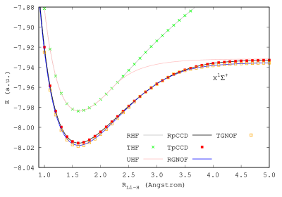
Figure 2: Potential energy curves obtained with the real (solid) and complex (dotted) versions of the HF, pCCD, and GNOF methods for the dissociation of the LiH molecule.

IV.3 When the complex (with time-reversal symmetry) and the real solutions differ.

While the time-reversal-symmetric complex and real solutions match for the H2 and the LiH systems across all bond lengths, this correspondence does not necessarily occur in other systems. To illustrate this, we have studied the PEC of BeH2 during the insertion of a beryllium atom into a hydrogen molecule. In Fig. 3(a), we have represented the reaction coordinate $x$ (in Bohr), where the Be atom is placed at the coordinate origin and the H atoms are located at $\pm y=2.54-0.46x$ with $x\in[0,4]$. This system has recently been used as a benchmark tool of different methods Ammar et al. (2024); Gaikwad et al. (2024); Mitxelena and Piris (2024); Gdanitz and Ahlrichs (1988); Mahapatra et al. (1998); Mahapatra, Datta, and Mukherjee (1999); Sharp and Gellene (2000); Kállay, Szalay, and Surján (2002); Pittner et al. (2004); Ruttink, Van Lenthe, and Todorov (2005); Lyakh, Ivanov, and Adamowicz (2006); Yanai and Chan (2006); Evangelista and Gauss (2010); Evangelista (2011); Evangelista and Gauss (2011) including the pCCD and RDMFT functional approximations, where the ability of these methods to account for non-dynamic electronic correlation effects was evaluated. For small values of $x>0$, the exact wave function is primarily governed by the electronic configuration $\ket{(1a_{1})^{2}(2a_{1})^{2}(1b_{2})^{2}}$. As $x$ increases, however, the configuration $\ket{(1a_{1})^{2}(2a_{1})^{2}(3a_{1})^{2}}$ becomes dominant. In the range $2.5<x<3$, the wave function undergoes a rapid transition from $\ket{(1a_{1})^{2}(2a_{1})^{2}(1b_{2})^{2}}$ to $\ket{(1a_{1})^{2}(2a_{1})^{2}(3a_{1})^{2}}$. Therefore, in the BeH2 system, the region $2.5\leq x\leq 3.5$ exhibits strong non-dynamic electronic correlation effects while the dynamic component is dominant for all other geometries.

Focusing on the consequences of using complex orbitals with time-reversal symmetry, we see in Fig. 3(b) that in regions where the dynamic electronic correlation effects are dominant the real and the complex solutions coincide. On the contrary, the flexibility provided by the complex natural orbital coefficients leads to a relaxation of the electronic density in the region where non-dynamic correlation effects are dominant (i.e., $x\in\left[2.5,3.5\right]$) making the complex solutions lie below the real ones for all methods studied. Let us first analyze the HF solutions. As we can observe, both solutions produce a smooth curve in the region where non-dynamic electronic correlation effects are dominant with the THF solution lying below the RHF one only on a very small interval. Using the real RHF orbitals to build the complex Hessian matrix [see Eq. (31)] in the interval where the solutions differ and proceeding to diagonalize it, we obtain one or two (depending on the geometry) negative eigenvalues. Since the gradient is still zero, this result indicates that the real solution is a stationary point (i.e., a saddle point) for the complex optimization problem. Thus, by re-optimizing the orbitals (and occupation numbers) we obtain the actual minimum. This result is comparable to the usual ones obtained with restricted and unrestricted methods for geometries beyond the Coulson-Fisher point. Burton (2020) However, as we show in Fig. 3(b), the THF energy lies above the real UHF one, which shows that the flexibility provided by the complex orbital coefficients is not sufficient to account for all the non-dynamic electronic correlation effects present.

To gain more insights into the THF solution, we have computed the spin-summed occupations numbers for the THF natural orbitals as a function of the reaction coordinate $x$. Note that this procedure is equivalent to the construction of the spin-summed unrestricted natural orbitals within the unrestricted HF formalism. Helgaker, Jorgensen, and Olsen (2000) To do so, we built

$$\boldsymbol{P}=\boldsymbol{c}_{\uparrow}^{\dagger}\cdot{}^{1}\boldsymbol{D}\cdot\boldsymbol{c}_{\uparrow}+\boldsymbol{c}_{\downarrow}^{\dagger}\cdot{}^{1}\boldsymbol{D}\cdot(\boldsymbol{c}_{\downarrow})$$ (37)

where $\boldsymbol{P}$ is the density matrix written in the real (scalar) atomic orbital basis $\psi$, $\boldsymbol{c}_{\uparrow}$ ($\boldsymbol{c}_{\downarrow}$) gathers the molecular orbital coefficients for the spin-up (spin-down) orbitals, and ${}^{1}\boldsymbol{D}$ is the HF first-order reduced density matrix (with ${}^{1}{D}_{pq}=\delta_{pq}$ for $p,q$ occupied and 0 otherwise). Then, using the Löwdin orthonormalization ($\boldsymbol{S}^{-1/2}\cdot\boldsymbol{P}\cdot\boldsymbol{S}^{-1/2}$ with $\boldsymbol{S}$ being the overlap matrix of the real (scalar) orbitals) and diagonalizing the resulting matrix, we obtained the THF natural orbitals and THF natural occupation numbers (${\boldsymbol{\eta}}$). In Fig. 3(d), we have plotted the spin-summed occupations numbers for the THF natural orbitals for the 3rd and 4th natural orbitals ($\eta_{3}$ and $\eta_{4}$). The $\eta_{1}$ and $\eta_{2}$ occupation numbers remain equal to 2 for all geometries. As we can observe in Fig. 3(d) in the region where non-dynamic correlation effects are dominant, $\eta_{3}$ and $\eta_{4}$ approach 1. Therefore, the THF is capable of retrieving some non-dynamic correlation effects present when compared to RHF, but its ability is limited and it is unable to perform as well as real UHF in this region (see Fig. 3(b)).

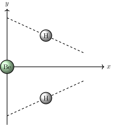
(a)

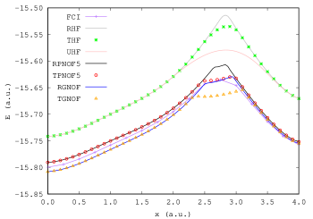
(b)

(c)

(d)

Figure 3: (a) Schematic representation of the insertion reaction of Be into H2 to form BeH2. The Be atom is placed at the origin and the hydrogen atoms are located at $\pm y=2.54-0.46x$. (b) Potential energy curves obtained with the real (solid) and complex (dotted) versions of HF, PNOF5, and GNOF methods for $0\leq x\leq 4$. The real UHF and the FCI curves are also included for comparison. (c) Changes in the spin-summed occupations numbers ($\eta_{3}$ and $\eta_{4}$) for the THF natural orbitals as functions of the reaction coordinate $x$. (d) Difference between the real and complex optimized electronic densities, $\rho(\boldsymbol{r})$, for the GNOF functional approximation along the insertion pathway for $x=2.75$ Bohr.

Moving to the PNOF5 and GNOF results, we also observe that the real and the complex solutions differ in the region where non-dynamic correlation effects are dominant. In the case of PNOF5, which is a fully $N$-representable method Garrod and Percus (1964); Mazziotti (2016) thanks to its correspondence with the constrained anti-symmetrized product of strongly orthogonal geminals, Pernal (2013) we notice that the TPNOF5 estimates (red dots) lie above the FCI energies. However, the TGNOF results (orange dots) lie below their FCI counterparts in the $x\in\left[2.5;3.5\right]$ interval, which indicates that this functional approximation can introduce $N$-representability violations when non-dynamic correlation effects are pronounced. Next, the analysis of the difference in the electronic density along the H-Be-H path for $x=2.75$ Bohr reveals that, for the GNOF functional, non-negligible changes occur in the vicinity of the nuclei and in the bonding region. (Similar results were obtained with the PNOF5 functional approximation.) Finally, let us mention that contrary to the HF case, the analysis of the eigenvalues of the complex Hessian matrix built with the RPNOF5 and RGNOF occupation numbers and orbitals revealed that the real solutions correspond to local minima for the complex optimization problem because all the eigenvalues obtained were positive.

To gain further insights into the complex solutions, let us analyze the THF as the non-relativistic limit of the Kramers’ restricted four-component DIRAC-HF (KR-4c-DHF) equation. Dyall and Fægri Jr (2007); Saue (2011); Hafner (1980) The KR-4c-DHF equation is the relativistic extension of the HF method for relativistic calculations, which produces 4c-spinors preserving time-reversal symmetry. It is known that the non-relativistic limit can be approached by setting the value of the speed of light $c$ to a large value in the 4c-DHF. Dyall and Fægri Jr (2007); Saue (2011); Pyykko (2012); Rodríguez-Mayorga et al. (2022) Then, as discussed in Sec. II, in this limit the KR-4c-DHF solution approaches the THF solution (instead of the RHF one) when the RHF and THF solutions differ because (i) the THF solution can be lower in energy, (ii) the THF and the KR-4c-DHF methods work with the extra flexibility provided by complex orbitals, and (iii) both methods are built to preserve time-reversal symmetry. To show this, we have taken the BeH2 system at the $x=2.75$ Bohr geometry, employed the cc-pVDZ basis set, Dunning Jr. (1989) and performed calculations using the DIRAC program Saue et al. (2020) setting the speed of light value to $c=10^{5}$. In the non-relativistic limit, the KR-4c-DHF energy ($-15.57555$ hartree) approaches the THF value ($-15.575600$ hartree), where for $c=10^{5}$ the energy difference is lower than $5\times 10^{-5}$ hartree (The RHF energy is $-15.563664$ hartree). This result illustrates that KR-4c-DHF solutions in the non-relativistic limit only approach the RHF ones when the RHF and the THF solutions are equivalent (which occurs in regions where non-dynamic correlation effects are not dominant). Otherwise, the KR-4c-DHF solutions in the non-relativistic limit may recover the THF values. Similar results were obtained for lowest singlet state of O2 at a distance of $R_{\text{O-O}}=10$ Å, where the RHF energy is $-149.33007$ hartree, the THF energy is $-149.41117$ hartree, and the KR-4c-DHF($c=10^{7}$) energy is $-149.41072$ hartree with the difference between the THF and the KR-4c-DHF being $4.5\times 10^{-4}$ hartree.

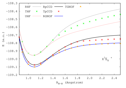
Figure 4: Potential energy curves obtained with the real (solid) and complex (dotted) versions of the HF, pCCD, and GNOF methods for the dissociation of the N2 molecule. The real UHF results are included for comparison.

Next, let us discuss another example where the real and complex solutions differ, the homolytic dissociation of the N2 molecule in its ground state, where three pairs of electrons are simultaneously broken. In Fig. 4 we have collected the real and complex HF, pCCD, and GNOF PECs. As one can observe, for all methods the real and complex solutions are equivalent up to $R_{\text{N-N}}\sim 1.4$ Å. Then, for larger interatomic distances, the real and the complex solutions differ, with the complex solution lying below the real one in all cases. As in the BeH2 example, the RHF is a saddle point of the complex solution when we evaluate the Hessian matrix. Again, the THF results can partially retrieve some non-dynamic electronic correlation effects but are still far from the UHF results. On the other hand, the GNOF real and complex results are very similar but the pCCD ones present large deviations, which shows that the difference between the real and the complex solutions is system- and method-dependent. Once more, as for the BeH2 system, all the eigenvalues of the complex Hessian matrix built with the real GNOF/pCCD occupation numbers/amplitudes and orbitals (multiplied by some random phases) were positive, which suggests that the real solutions correspond to local minima of the complex optimization problem for the RDMFT functional approximations and the pCCD method.

V Conclusions

In this work, we have presented and discussed the consequences of using complex orbitals including time-reversal symmetry in RDMFT and pCCD calculations. From a theoretical perspective, the RDMFT $JKL$-only functional approximations and the pCCD method reduce to $JK$-only methods where only the Hartree and exchange integrals are needed to evaluate the energy. Specifically, for spin-compensated systems, the energy expression is given by

$$E^{\text{TPNOFs/TGNOF/TpCCD}}=2\sum_{p}n_{p}h_{pp}+\sum_{pq}\left({}^{2}D_{pq,pq}J_{pq}+^{2}D_{pq,qp}K_{pq}\right).$$ (38)

This simplification occurs because the $L$ integrals that accompany opposite-spin interactions become $K$ integrals when time-reversal symmetry is considered. Consequently, the $t$ and $z$ amplitudes of TpCCD are also real-valued. Note that Eq. (38) is also applicable for other methods that use $JKL$-only integrals such as the antisymmetrized product of strongly orthogonal geminals, Pernal (2013) the $\Delta$NO method, Hollett, Hosseini, and Menzies (2016); Elayan, Gupta, and Hollett (2022) and the recently proposed methodology based on Richardson-Gaudin states. Fecteau et al. (2020, 2021); Johnson (2023) Another major advantage of including time-reversal symmetry is that the Piris-Ugalde orbital optimization algorithm can be applied to problems involving complex orbitals. This is because the diagonal terms of the gradient responsible for changing the orbital phase vanish ($g_{pp}=0$). This advantage can be further exploited in future implementations of the Piris RDMFT functional approximations and pCCD methods for extended systems where several complex one-body Bloch states are required. In such cases, quadratic convergent algorithms that require the Hessian matrix become computationally prohibitive. Therefore, this work sheds light on the technical and theoretical aspects encountered when implementing the Piris RDMFT functional approximations and pCCD methods for extended systems.

From a practical perspective, our numerical examples reveal that the real and complex solutions may differ in regions where non-dynamic correlation effects are enhanced with complex energies lying below the real ones in such cases. In the case of HF calculations, the real solutions correspond to saddle points of the complex optimization problem. On the other hand, for RDMFT functional approximations and the pCCD method, the real solutions are local minima. Interestingly, the TGNOF energies may lie below the FCI ones in regions dominated by non-dynamic correlation effects, suggesting that this functional approximation introduces $N$-representability violations. Finally, we have shown that the THF solution corresponds to the non-relativistic limit of the KR-4c-DHF method, where the RHF solution is attained only when it is equivalent to the THF one in regions where the non-dynamic electronic correlation effects are not dominant.

Supplementary Material

The Supplementary Material for the present article includes the H2 case, where the RPNOF5 and TPNOF5 solutions coincide.

Data Availability

The data that support the findings of this study are available within the article and its supplementary material.

Appendix A Appendix A: The real RDMFT and pCCD Hessian

For real orbitals, the one- and two-electron integrals, the occupation numbers, second-order reduced density matrix elements, and the parameters $\kappa_{pq}$ are real. For restricted calculations, only the elements $\kappa_{pq}$ with $p>q$ are unique. Hence, we have

$$\hat{\kappa}=\sum_{p>q}\sum_{\sigma}\kappa_{pq}({\hat{c}^{\dagger}}_{p\sigma}{\hat{c}^{\vphantom{\dagger}}}_{q\sigma}-{\hat{c}^{\dagger}}_{q\sigma}{\hat{c}^{\vphantom{\dagger}}}_{p\sigma}),$$ (39)

only the $g_{pq}$ for $p>q$ elements of the gradient are needed, and only $p>q$ and $r>s$ terms of the Hessian are required. The Hessian is generally a Hermitian matrix (symmetric in the real case); thus, its construction only requires building the upper diagonal part and applying the symmetry conditions. In the case of RDMFT and pCCD calculations, the construction of the Hessian scales as $M^{5}$, which makes it reasonable in terms of computational cost when compared with more complex methods where the construction of the Hessian scales as $M^{7}$. The Hessian for real orbitals in terms of the auxiliary ${\bf\tilde{G}}$ matrix elements takes the following form

$$G_{pq,rs} =\partialderivative{E(\boldsymbol{\kappa})}{\kappa_{pq}}{\kappa_{rs}}=\tilde{G}_{pq,rs}-\tilde{G}_{qp,rs}-\tilde{G}_{pq,sr}+\tilde{G}_{qp,sr}$$ (40)

that are evaluated using Eq. (32). Notice that the real Hessian is given by the first four elements of Eq. (31) because they correspond to partial derivatives taken with respect to $\real\kappa_{pq}$ elements. Finally, for completeness, let us mention that the 6th to the 8th elements in Eq. (31) are obtained with partial derivatives with respect to $\imaginary\kappa_{pq}$ while the third line is produced by crossed $\real\kappa_{pq}$ and $\imaginary\kappa_{pq}$ derivatives.

References

- Löwdin (1955) P.-O. Löwdin, Phys. Rev. 97, 1474 (1955).
- Cioslowski (1991) J. Cioslowski, Phys. Rev. A 43, 1223 (1991).
- Helgaker, Jorgensen, and Olsen (2000) T. Helgaker, P. Jorgensen, and J. Olsen, Molecular Electronic Structure Theory (Wiley, Chichester, 2000).
- Malmqvist and Roos (1989) P.-Å. Malmqvist and B. O. Roos, Chem. Phys. Lett. 155, 189 (1989).
- Roos, Taylor, and Sigbahn (1980) B. O. Roos, P. R. Taylor, and P. E. Sigbahn, Chem. Phys. 48, 157 (1980).
- Roos (1980) B. O. Roos, Int. J. Quant. Chem. 18, 175 (1980).
- Roos (2005) B. O. Roos, in Theory and Applications of Computational Chemistry (Elsevier, 2005) pp. 725–764.
- White (1992) S. R. White, Phys. Rev. Lett. 69, 2863 (1992).
- White (1993) S. R. White, Phys. Rev. B 48, 10345 (1993).
- Chan and Sharma (2011) G. K.-L. Chan and S. Sharma, Annual review of physical chemistry 62, 465 (2011).
- Baiardi and Reiher (2020) A. Baiardi and M. Reiher, J. Chem. Phys. 152 (2020).
- Gilbert (1975) T. L. Gilbert, Phys. Rev. B 12, 2111 (1975).
- Valone (1991) S. M. Valone, Phys. Rev. B 44, 1509 (1991).
- Henderson et al. (2014) T. Henderson, I. Bulik, T. Stein, and G. Scuseria, J. Chem. Phys. 141 (2014).
- Piris (2013a) M. Piris, Int. J. Quant. Chem. 113, 620 (2013a).
- Piris (2018) M. Piris, Phys. Rev. A 98, 022504 (2018).
- Piris (2021) M. Piris, Phys. Rev. Lett. 127, 233001 (2021).
- Mitxelena and Piris (2020a) I. Mitxelena and M. Piris, J. Phys. Condens. Matter 32, 17LT01 (2020a).
- Mitxelena and Piris (2020b) I. Mitxelena and M. Piris, J. Chem. Phys. 152, 064108 (2020b).
- Mitxelena and Piris (2024) I. Mitxelena and M. Piris, J. Chem. Phys. 160 (2024).
- Rodríguez-Mayorga, Giesbertz, and Visscher (2022) M. Rodríguez-Mayorga, K. Giesbertz, and L. Visscher, SciPost Chem. 1, 4 (2022).
- Boguslawski et al. (2012) K. Boguslawski, P. Tecmer, O. Legeza, and M. Reiher, J. Phys. Chem. Lett. 3, 3129 (2012).
- Boguslawski (2021) K. Boguslawski, Chem. Comm. 57, 12277 (2021).
- Nowak, Legeza, and Boguslawski (2021) A. Nowak, Ö. Legeza, and K. Boguslawski, J. Chem. Phys. 154, 084111 (2021).
- Gałynśka and Boguslawski (2024) M. Gałynśka and K. Boguslawski, J. Chem. Theory Comput. , 4182 (2024).
- Kossoski and Loos (2023) F. Kossoski and P.-F. Loos, J. Chem. Theory Comput. 19, 8654 (2023).
- Kossoski et al. (2021) F. Kossoski, A. Marie, A. Scemama, M. Caffarel, and P.-F. Loos, J. Chem. Theory Comput. 17, 4756 (2021).
- Ravi et al. (2023) M. Ravi, A. Perera, Y. C. Park, and R. J. Bartlett, J. Chem. Phys. 159, 094101 (2023).
- Marie, Kossoski, and Loos (2021) A. Marie, F. Kossoski, and P.-F. Loos, J. Chem. Phys. 155 (2021).
- Muller and Willner (1993) H. S. Muller and H. Willner, J. Phys. Chem. 97, 10589 (1993).
- Sharma et al. (2008) S. Sharma, J. K. Dewhurst, N. N. Lathiotakis, and E. K. U. Gross, Phys. Rev. B 78, 201103 (2008).
- Cioslowski and Pernal (2000) J. Cioslowski and K. Pernal, Phys. Rev. A 61, 034503 (2000).
- Sharma et al. (2013) S. Sharma, J. Dewhurst, S. Shallcross, and E. Gross, Phys. Rev. Lett. 110, 116403 (2013).
- Cullen (1996) J. Cullen, Chem. Phys. 202, 217 (1996).
- Stein, Henderson, and Scuseria (2014) T. Stein, T. M. Henderson, and G. E. Scuseria, J. Chem. Phys. 140 (2014).
- Kutzelnigg (2012) W. Kutzelnigg, Chem. Phys. 401, 119 (2012).
- Voorhis and Head-Gordon (2000) T. V. Voorhis and M. Head-Gordon, J. Chem. Phys. 112, 5633 (2000).
- Van Voorhis and Head-Gordon (2001) T. Van Voorhis and M. Head-Gordon, J. Chem. Phys. 115, 7814 (2001).
- Small and Head-Gordon (2012) D. W. Small and M. Head-Gordon, J. Chem. Phys. 137 (2012).
- Fukutome (1981) H. Fukutome, Int. J. Quant. Chem. 20, 955 (1981).
- Scuseria et al. (2011) G. E. Scuseria, C. A. Jiménez-Hoyos, T. M. Henderson, K. Samanta, and J. K. Ellis, J. Chem. Phys. 135, 124108 (2011).
- Jiménez-Hoyos et al. (2012) C. A. Jiménez-Hoyos, T. M. Henderson, T. Tsuchimochi, and G. E. Scuseria, J. Chem. Phys. 136, 164109 (2012).
- Small, Sundstrom, and Head-Gordon (2015) D. W. Small, E. J. Sundstrom, and M. Head-Gordon, J. Chem. Phys. 142, 024104 (2015).
- Jiménez-Hoyos, Henderson, and Scuseria (2011) C. A. Jiménez-Hoyos, T. M. Henderson, and G. E. Scuseria, J. Chem. Theory Comput. 7, 2667 (2011).
- Song, Henderson, and Scuseria (2004) R. Song, T. M. Henderson, and G. E. Scuseria, arXiv:2405.06776 (2004).
- Stuber and Paldus (2003) J. L. Stuber and J. Paldus, Symmetry breaking in the independent particle model in Fundamental World of Quantum Chemistry (Springer Netherlands, 2003) pp. 67–139.
- Note (1) Note1, This option is not included in Ref. Jiménez-Hoyos, Henderson, and Scuseria, 2011, where real coefficients are employed, time-reversal symmetry is preserved, but not .
- Gonze et al. (2020) X. Gonze, B. Amadon, G. Antonius, F. Arnardi, L. Baguet, J.-M. Beuken, et al., Comp. Phys. Com. 248, 107042 (2020).
- Giannozzi et al. (2009) P. Giannozzi, S. Baroni, N. Bonini, M. Calandra, R. Car, C. Cavazzoni, D. Ceresoli, G. L. Chiarotti, M. Cococcioni, I. Dabo, et al., J. Phys. Condens. Matter 21, 395502 (2009).
- Giannozzi et al. (2017) P. Giannozzi, O. Andreussi, T. Brumme, O. Bunau, M. B. Nardelli, M. Calandra, R. Car, C. Cavazzoni, D. Ceresoli, M. Cococcioni, et al., J. Phys. Condens. Matter 29, 465901 (2017).
- Denawi et al. (2023) A. Denawi, F. Bruneval, M. Torrent, and M. Rodríguez-Mayorga, Phys. Rev. B 108, 125107 (2023).
- Dyall and Fægri Jr (2007) K. Dyall and K. Fægri Jr, Introduction to relativistic quantum chemistry (Oxford University Press, 2007).
- Kramers (1930) H. A. Kramers, Proc. Acad. Amst 33 (1930).
- Aucar, Jensen, and Oddershede (1995) G. Aucar, H. A. Jensen, and J. Oddershede, Chem. Phys. Lett. 232, 47 (1995).
- Bučinskỳ et al. (2015) L. Bučinskỳ, M. Malček, S. Biskupič, D. Jayatilaka, G. E. Büchel, and V. B. Arion, Comput. Theor. Chem. 1065, 27 (2015).
- Bučinskỳ, Malček, and Biskupič (2016) L. Bučinskỳ, M. Malček, and S. Biskupič, Int. J. Quant. Chem. 116, 1040 (2016).
- Komorovsky, Repisky, and Bučinskỳ (2016) S. Komorovsky, M. Repisky, and L. Bučinskỳ, Phys. Rev. A 94, 052104 (2016).
- (58) H. J. Aa. Jensen, Douglas–Kroll the Easy Way, Talk at Conference on Relativistic Effects in Heavy Elements - REHE, Mülheim, Germany, April (2005).
- Kutzelnigg and Liu (2005) W. Kutzelnigg and W. Liu, J. Chem. Phys. 123, 241102 (2005).
- Iliaš and Saue (2007) M. Iliaš and T. Saue, J. Chem. Phys. 126 (2007).
- Piris and Ugalde (2009) M. Piris and J. Ugalde, J. Comput. Chem. 30, 2078 (2009).
- Hohenberg and Kohn (1964) P. Hohenberg and W. Kohn, Phys. Rev. 136, B864 (1964).
- Burke and friends (2007) K. Burke and friends, The ABC of DFT (Department of Chemistry, University of California, Irvine, California, 2007).
- Müller (1984) A. M. K. Müller, Phys. Lett. 105A, 446 (1984).
- Buijse and Baerends (2002) M. A. Buijse and E. J. Baerends, Mol. Phys. 100, 401 (2002).
- Buijse (1991) M. A. Buijse, Thesis: Electron Correlation. Fermi and Coulomb holes, dynamical and nondynamical correlation, Ph.D. thesis, Vrije Universiteit, Amsterdam, The Netherlands (1991).
- Rodríguez-Mayorga et al. (2017) M. Rodríguez-Mayorga, E. Ramos-Cordoba, M. Via-Nadal, M. Piris, and E. Matito, Phys. Chem. Chem. Phys. 19, 24029 (2017).
- Piris (2013b) M. Piris, J. Chem. Phys. 139, 064111 (2013b).
- Piris (2017) M. Piris, Phys. Rev. Lett. 119, 063002 (2017).
- Piris (1999) M. Piris, J. Math. Chem. 25, 47 (1999).
- Lathiotakis, Gidopoulos, and Helbig (2010) N. N. Lathiotakis, N. I. Gidopoulos, and N. Helbig, J. Chem. Phys. 132, 084105 (2010).
- Cioslowski, Piris, and Matito (2015) J. Cioslowski, M. Piris, and E. Matito, J. Chem. Phys. 143, 214101 (2015).
- Jensen and Jorgensen (1984) H. J. A. Jensen and P. Jorgensen, J. Chem. Phys. 80, 1204 (1984).
- Yamaguchi et al. (1990) Y. Yamaguchi, I. L. Alberts, J. D. Goddard, and H. F. Schaefer III, Chem. Phys. 147, 309 (1990).
- Elayan, Gupta, and Hollett (2022) I. A. Elayan, R. Gupta, and J. W. Hollett, J. Chem. Phys. 156 (2022).
- Nottoli, Gauss, and Lipparini (2021) T. Nottoli, J. Gauss, and F. Lipparini, J. Chem. Theory Comput. 17, 6819 (2021).
- Cartier and Giesbertz (2024) N. Cartier and K. Giesbertz, J. Chem. Theory Comput. 20, 3669 (2024).
- Herbert and Harriman (2003) J. M. Herbert and J. E. Harriman, J. Chem. Phys. 118, 10835 (2003).
- Visscher and Dyall (1995) L. Visscher and K. G. Dyall, Int. J. Quant. Chem. 29, 411 (1995).
- Burton and Wales (2020) H. Burton and D. Wales, J. Chem. Theory Comput. 17, 151 (2020).
- Douady et al. (1980) J. Douady, Y. Ellinger, R. Subra, and B. Levy, J. Chem. Phys. 72, 1452 (1980).
- Jensen and Ågren (1986) H. J. A. Jensen and H. Ågren, Chem. Phys. 104, 229 (1986).
- Helgaker et al. (1986) T. Helgaker, J. Almlöf, H. Jensen, and P. Jo/rgensen, J. Chem. Phys. 84, 6266 (1986).
- Kreplin, Knowles, and Werner (2020) D. Kreplin, P. Knowles, and H.-J. Werner, J. Chem. Phys. 152 (2020).
- Vidal et al. (2024) L. Vidal, T. Nottoli, F. Lipparini, and E. Cancès, J. Phys. Chem. A 128 (2024).
- Lew-Yee, Piris, and M. del Campo (2021) J. H. Lew-Yee, M. Piris, and J. M. del Campo, J. Chem. Phys. 154, 064102 (2021).
- Bruneval et al. (2016) F. Bruneval, T. Rangel, S. Hamed, M. Shao, C. Yang, and J. Neaton, Comp. Phys. Comm. 208, 149 (2016).
- Rodríguez-Mayorga (2022) M. Rodríguez-Mayorga, “Standalone NOFT module (1.0) published on Zenodo,” (2022).
- Piris and Mitxelena (2021) M. Piris and I. Mitxelena, Comp. Phys. Comm. 259, 107651 (2021).
- Dunning Jr. (1989) T. Dunning Jr., J. Chem. Phys. 90, 1007 (1989).
- Evangelista and Gauss (2010) F. A. Evangelista and J. Gauss, J. Chem. Phys. 133 (2010).
- Ammar et al. (2024) A. Ammar, A. Marie, M. Rodríguez-Mayorga, H. G. Burton, and P.-F. Loos, J. Chem. Phys. 160 (2024).
- Perdew, Burke, and Ernzerhof (1996) J. Perdew, K. Burke, and M. Ernzerhof, Phys. Rev. Lett. 77, 3865 (1996).
- Rodríguez-Mayorga et al. (2016) M. Rodríguez-Mayorga, E. Ramos-Cordoba, P. Salvador, M. Solà, and E. Matito, Mol. Phys. 114, 1345 (2016).
- Gaikwad et al. (2024) P. Gaikwad, T. Kim, M. Richer, R. Lokhande, G. Sánchez-Díaz, P. Limacher, P. Ayers, and R. A. Miranda-Quintana, J. Chem. Phys. 160 (2024).
- Gdanitz and Ahlrichs (1988) R. J. Gdanitz and R. Ahlrichs, Chem. Phys. Lett. 143, 413 (1988).
- Mahapatra et al. (1998) U. S. Mahapatra, B. Datta, B. Bandyopadhyay, and D. Mukherjee, in Advances in quantum chemistry, Vol. 30 (Elsevier, 1998) pp. 163–193.
- Mahapatra, Datta, and Mukherjee (1999) U. S. Mahapatra, B. Datta, and D. Mukherjee, J. Chem. Phys. 110, 6171 (1999).
- Sharp and Gellene (2000) S. B. Sharp and G. I. Gellene, J. Phys. Chem. A 104, 10951 (2000).
- Kállay, Szalay, and Surján (2002) M. Kállay, P. G. Szalay, and P. R. Surján, J. Chem. Phys. 117, 980 (2002).
- Pittner et al. (2004) J. Pittner, H. V. Gonzalez, R. J. Gdanitz, and P. Čársky, Chem. Phys. Lett. 386, 211 (2004).
- Ruttink, Van Lenthe, and Todorov (2005) P. Ruttink, J. Van Lenthe, and P. Todorov, Mol. Phys. 103, 2497 (2005).
- Lyakh, Ivanov, and Adamowicz (2006) D. I. Lyakh, V. V. Ivanov, and L. Adamowicz, Theor. Chim. Acta (Berlin) 116, 427 (2006).
- Yanai and Chan (2006) T. Yanai and G. K. Chan, J. Chem. Phys. 124 (2006).
- Evangelista (2011) F. A. Evangelista, J. Chem. Phys. 134 (2011).
- Evangelista and Gauss (2011) F. A. Evangelista and J. Gauss, J. Chem. Phys. 134 (2011).
- Burton (2020) H. Burton, Holomorphic Hartree-Fock Theory: Moving Beyond the Coulson-Fischer Point, Ph.D. thesis (2020).
- Garrod and Percus (1964) C. Garrod and J. Percus, J. Math. Phys. 5, 1756 (1964).
- Mazziotti (2016) D. Mazziotti, Phys. Rev. A 94, 032516 (2016).
- Pernal (2013) K. Pernal, Comput. Theor. Chem. 1003, 127 (2013).
- Saue (2011) T. Saue, Chem. Phys. Chem. 12, 3077 (2011).
- Hafner (1980) P. Hafner, J. Phys. B 13, 3297 (1980).
- Pyykko (2012) P. Pyykko, Chem. Rev. 112, 371 (2012).
- Rodríguez-Mayorga et al. (2022) M. Rodríguez-Mayorga, D. Keizer, K. Giesbertz, and L. Visscher, J. Chem. Phys. 157 (2022).
- Saue et al. (2020) T. Saue, R. Bast, A. S. P. Gomes, H. J. A. Jensen, L. Visscher, I. A. Aucar, R. Di Remigio, K. G. Dyall, E. Eliav, E. Fasshauer, et al., J. Chem. Phys. 152, 204104 (2020).
- Note (2) Note2, Similar results were obtained for lowest singlet state of \ceO2 at a distance of Å, where the RHF energy is hartree, the THF energy is hartree, and the KR-4c-DHF() energy is hartree with the difference between the THF and the KR-4c-DHF being hartree.
- Hollett, Hosseini, and Menzies (2016) J. W. Hollett, H. Hosseini, and C. Menzies, J. Chem. Phys. 145 (2016).
- Fecteau et al. (2020) C.-É. Fecteau, H. Fortin, S. Cloutier, and P. A. Johnson, J. Chem. Phys. 153 (2020).
- Fecteau et al. (2021) C.-É. Fecteau, F. Berthiaume, M. Khalfoun, and P. A. Johnson, J. Math. Chem. 59, 289 (2021).
- Johnson (2023) P. A. Johnson, arXiv:2312.08804 (2023).