Open-World Reinforcement Learning over
Long Short-Term Imagination

Abstract

Training visual reinforcement learning agents in a high-dimensional open world presents significant challenges. While various model-based methods have improved sample efficiency by learning interactive world models, these agents tend to be “short-sighted”, as they are typically trained on short snippets of imagined experiences. We argue that the primary obstacle in open-world decision-making is improving the efficiency of off-policy exploration across an extensive state space. In this paper, we present LS-Imagine, which extends the imagination horizon within a limited number of state transition steps, enabling the agent to explore behaviors that potentially lead to promising long-term feedback. The foundation of our approach is to build a long short-term world model. To achieve this, we simulate goal-conditioned jumpy state transitions and compute corresponding affordance maps by zooming in on specific areas within single images. This facilitates the integration of direct long-term values into behavior learning. Our method demonstrates significant improvements over state-of-the-art techniques in MineDojo.

1 Introduction

Open-world decision-making in the context of reinforcement learning (RL) involves the following characteristics: 1) The agent operates within an interactive environment that features a vast state space; 2) The learned policy presents a high degree of flexibility, allowing interaction with various objects in the environment; 3) The agent lacks full visibility of the internal states and physical dynamics of the external world, meaning that its perception of the environment (e.g., raw images) carries substantial uncertainty. For example, Minecraft serves as a typical open-world game.

Building upon recent progress in visual control, open-world decision-making aims to train agents to approach human-level intelligence based solely on high-dimensional visual observations. However, this presents significant challenges. For example, in Minecraft tasks, existing methods like Voyager (Wang et al., 2024a) employ specific Minecraft APIs as the high-level controller, which is incompatible with standard visual control settings. While approaches such as PPO-with-MineCLIP (Fan et al., 2022) and DECKARD (Nottingham et al., 2023) perform low-level visual control, these model-free RL methods struggle to grasp the underlying mechanics of the environment. This may result in high trial-and-error costs, leading to inefficiencies in both exploration and sample usage. Although DreamerV3 (Hafner et al., 2023) employs a model-based RL (MBRL) approach to improve sample efficiency, it is often “short-sighted” since the policy is optimized using short-term experiences—typically $15$ time steps—generated by the world model. The absence of long-term guidance significantly hampers an effective exploration of the vast solution space of the open world.

To improve the behavior learning efficiency of MBRL, in this paper, we introduce a novel method named Long Short-Term Imagination (LS-Imagine). Our key approach involves enabling the world model to efficiently simulate the long-term effects of specific behaviors without the need for repeatedly rolling out one-step predictions. As illustrated in Figure 1, once trained, the world model provides both instant and jumpy state transitions along with corresponding (intrinsic) rewards, facilitating policy optimization in a joint space of short- and long-term imaginations. This encourages the agent to explore behaviors that lead to promising long-term outcomes.

The foundation of LS-Imagine is to train a long short-term world model, which requires integrating task-specific guidance into the representation learning phase based on off-policy experience replay. However, this creates a classic “chicken-and-egg” dilemma: without true data showing the agent has reached the goal, how can we effectively train the model to simulate jumpy transitions from current states to pivotal future states that suggest a high likelihood of achieving that goal? To address this issue, we first continuously zoom in on individual images to simulate the consecutive video frames as the agent approaches the goal. We then generate affordance maps by evaluating the relevance of the pseudo video to task-specific goals presented in textual instructions, using the established MineCLIP reward model (Fan et al., 2022). Subsequently, we train specific branches of the world model to capture both instant and jumpy state transitions, using pairs of image observations from adjacent time steps as well as those across longer intervals. Finally, we optimize the agent’s policy based on a finite sequence of imagined latent states generated by the world model, integrating a more direct estimate of long-term values into decision-making.

Let’s use the example in Figure 1 to further elaborate the novel aspects of the behavior learning process: After receiving the instruction “cut a tree”, the agent simulates near-future states based on the current real observation. It initially performs several single-step rollouts until it identifies a point in time for a long-distance state jump that allows it to approach the tree. The agent then executes this jump and optimizes its policy network to maximize the long-sight value function.

We evaluate our approach in the challenging open-world tasks from MineDojo (Fan et al., 2022). LS-Imagine demonstrates superior performance compared to existing visual RL methods.

The contributions of this work are summarized as follows:

• We present a novel model-based RL method that captures both instant and jumpy state transitions and leverages them in behavior learning to improve exploration efficiency in the open world.

• Our approach presents four concrete contributions: (i) a long short-term world model architecture, (ii) a method for generating affordance maps through image zoom-in, (iii) a novel form of intrinsic rewards based on the affordance map, and (iv) an improved behavior learning method that integrates long-term values and operates on a mixed long short-term imagination pathway.

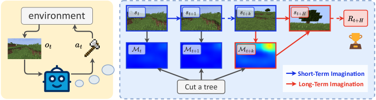
Figure 1: The general framework of LS-Imagine, an MBRL agent that operates solely on raw pixels. The fundamental idea is to extend the imagination horizon within a limited number of state transition steps, enabling the agent to explore behaviors that potentially lead to promising long-term feedback.

2 Problem Formulation

We solve visual reinforcement learning as a partially observable Markov decision process (POMDP), using MineDojo as the test bench. Specifically, our method manipulates low-dimensional control signals $a_{t}$ while receiving only sequential high-dimensional visual observations $o_{<t}$ and episodic sparse rewards $r^{e}$, without access to the internal APIs of the open-world games. In comparison, as shown in Table 1, existing Minecraft agents present notable distinctions in learning paradigms (i.e., controller), observation data, and the use of expert demonstrations.

In our formulation, the world model is learned on the replayed data consisting of so-called short-term tuples $\{\mathcal{D}_{t}=(o_{t},a_{t},r_{t},c_{t},\mathcal{M}_{t},j_{t},\Delta_{t},G_{t})\}$ and long-term tuples $\{\mathcal{D}^{\prime}_{t}=(o_{t}^{\prime},a_{t}^{\prime},{r}_{t}^{\prime},\mathcal{M}^{\prime}_{t},c_{t}^{\prime},j_{t}^{\prime},\Delta_{t}^{\prime},G_{t}^{\prime})\}$, where $c_{t}$ denotes the episode continuation flag, $\mathcal{M}_{t}$ denotes the affordance map, $j_{t}$ denotes the jumping flag, $\Delta_{t}$ denotes the number of environment steps between state transitions, and $G_{t}$ denotes the cumulative discounted reward over this period. The policy is learned on trajectories of long short-term imaginations $\{(h_{t},\hat{z}_{t},a_{t},\hat{r}_{t},\hat{c}_{t},\hat{j}_{t},\hat{\Delta}_{t},\hat{G}_{t})\}$, where $h_{t}$ denotes the deterministic recurrent state and $z_{t}$ denotes the stochastic state.

Table 1: Experimental setups of the Minecraft AI agents. IL is short for imitation learning.

Model	Controller	Observation	Video Demos
DECKARD (2023)	RL	Pixels & Inventory	✓
Auto MC-Reward (2024a)	IL + RL	Pixels & GPS	✗
Voyager (2024a)	GPT-4	Minecraft simulation & Error trace	✗
DEPS (2023)	IL	Pixels & Yaw/pitch angle & GPS & Voxel	✗
STEVE-1 (2023)	Generative model	Pixels	✗
VPT (2022)	IL + RL	Pixels	✓
DreamerV3 (2023)	RL	Pixels	✗
LS-Imagine	RL	Pixels	✗

3 Method

3.1 Overview of LS-Imagine

In this section, we present the details of LS-Imagine, which involves the following algorithm steps, including world model learning, behavior learning, and environment interaction:

1. Affordance map computation (Sec. 3.2.1): We employ a sliding bounding box to scan individual images and execute continuous zoom-ins inside the bounding box, simulating consecutive video frames that correspond to long-distance state transitions. We then create affordance maps by assessing the relevance of the fake video clips to task-specific goals expressed in text using the established MineCLIP reward model (Fan et al., 2022).

2. Rapid affordance map generation (Sec. 3.2.2): Given that affordance maps will be frequently used in subsequent Step 5 to evaluate the necessities for jumpy state transitions, we train a U-Net module to approximate the affordance maps annotated in Step 1 for the sake of efficiency.

3. World model training (Sec. 3.3): We train the world model to capture short- and long-term state transitions, using replay data with high responses from the affordance map. Each trajectory from the buffer includes pairs of samples from both adjacent time steps and long-distance intervals.

4. Behavior learning (Sec. 3.4): We perform an actor-critic algorithm to optimize the agent’s policy based on a finite sequence of long short-term imaginations generated by the world model.

5. Data update: We apply the agent to interact with the environment and gather new data. Next, we leverage the generated affordance map to efficiently filter sample pairs suitable for long-term modeling, incorporating both short- and long-term sample pairs to update the replay buffer.

6. Iterate Steps 3–5.

Below, we discuss the specific operations for each training step. For a complete description of the full training algorithm, please refer to Alg. 1 in the Appendix D.

3.2 Affordance Map and Intrinsic Reward

We generate affordance maps using visual observations and textual task definitions to improve the sample efficiency of model-based reinforcement learning in open-world tasks. The core idea is to direct the agent’s attention to task-relevant areas of the visual observation, leading to higher exploration efficiency. Let $\mathcal{M}_{o_{t},I}(w,h)$ be the affordance map that represents the potential exploration value at pixel position $(w,h)$ on the image observation $o_{t}$, given textual instruction $I$ (e.g., “cut a tree”). The affordance map highlights the relevance between regions of the observation and the task description, serving as a spatial prior that effectively directs the agent’s exploration toward areas of interest.

3.2.1 Affordance Map Computation via Virtual Exploration

To create the affordance map, as shown in Figure 2(a), we simulate and evaluate the agent’s exploration without relying on real successful trajectories. Concretely, we first adopt a random agent to interact with task-specific environments for data collection. Starting with the agent’s observation $o_{t}$ at time step $t$, we use a sliding bounding box with dimensions scaled to $15\%$ of the observation’s width and height to traverse the entire observation from left to right and top to bottom. The sliding bounding box moves horizontally and vertically in $9$ steps, respectively, covering every potential region in both dimensions. For each position on the sliding bounding box of the observation $o_{t}$, we crop $16$ images from $o_{t}$. These cropped images narrow the field of view to focus on the region and are resized back to the original image dimensions. These resized images are denoted as $x_{t}^{k}$ (where $0\leq k<16$). The ordered set $\mathcal{X}_{t}=[x_{t}^{k}\mid k=0,1,\ldots,15]$ represents a sequence of $16$ frames simulating the visual transition as the agent moves towards the position specified by the current sliding bounding box. Subsequently, we employ the MineCLIP model to calculate the correlation between the $\mathcal{X}_{t}$ of images, simulating the virtual exploration process, and the task description $I$. In this way, we quantify the affordance value of the sliding bounding box, indicating the potential exploration interest of the area.

After calculating the correlation score for each sliding bounding box, we fuse these values to obtain a smooth affordance map $\mathcal{M}_{o_{t},I}$. For pixels that are covered by multiple sliding bounding boxes due to overlapping regions, the integrated affordance value is obtained by averaging the values from all the overlapping windows.

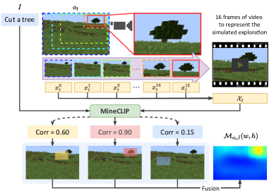
(a) Affordance map calculation

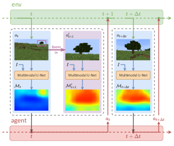
(b) Rapid affordance map generation

Figure 2: The two steps for on-the-fly affordance map estimation: (a) Simulate exploration via image zoom-in and calculate the task-correlation scores of the virtual explorations using MineCLIP. (b) Learn to generate affordance maps more efficiently using a multimodal U-Net.

3.2.2 Multimodal U-Net for Rapid Affordance Map Generation

The annotation of affordance maps, as previously described, involves extensive window traversal and computations for each window position using a pre-trained video-text alignment model. This method is computationally demanding and time-consuming, making real-time applications challenging.

To address this issue, we first use a random agent to interact with the environment for data collection. Next, we annotate the affordance maps for the collected images using the aforementioned method based on virtual exploration. We gather a dataset of tuples ($o_{t},I,\mathcal{M}_{o_{t},I}$) and use it to train a multimodal U-Net, building upon the Swin-Unet architecture (Cao et al., 2022). To handle multimodal inputs effectively, we extract text features from the language instructions and image features from the downsampling process of Swin-Unet, and then fuse them with multi-head attention. For architecture details of the proposed model, please refer to Figure 9 in the Appendix. In this way, with the pretrained multimodal U-Net, we can efficiently generate affordance maps at each time step using visual observations and language instructions.

3.2.3 Affordance-Driven Intrinsic Reward

To leverage the task-relevant prior knowledge presented by the affordance map for efficient exploration in the open world, we introduce the following intrinsic reward function:

$$r^{i}_{t}=\frac{1}{WH}\sum_{w=1}^{W}\sum_{h=1}^{H}\mathcal{M}_{o_{t},I}(w,h)\cdot\mathcal{G}(w,h),$$ (1)

where $W$ and $H$ denote the width and height of the visual observation, respectively. $\mathcal{G}(w,h)$ represents a Gaussian matrix with the same dimensions as the affordance map. Consequently, the agent receives a composite reward consisting of the episodic sparse reward from the environment, the reward from MineCLIP (Fan et al., 2022), and the intrinsic reward from the affordance map:

$$r_{t}=r^{e}+r_{t}^{\text{MineCLIP}}+\alpha r_{t}^{i},$$ (2)

where $\alpha$ is a hyperparameter. In contrast to the MineCLIP reward, which relies on the agent’s past performance, our affordance-driven intrinsic reward emphasizes long-term values derived from future virtual exploration. It encourages the agent to adjust the policy to pursue task-related targets when they appear in its view, ensuring these targets are centrally positioned in future visual observations to maximize this reward function.

3.3 Long Short-Term World Model

3.3.1 Learning Jumping Flags

In LS-Imagine, the world model is customized for long-term and short-term state transitions. It decides which type of transition to adopt based on the current state and predicts the next state with the selected transition branch. To facilitate the switch between long-term and short-term state transitions, we introduce a jumping flag $j_{t}$, which indicates whether a jumpy transition or long-term state transition, should be adopted at time step $t$. When a distant task-related target appears in the agent’s observation, which can be reflected by a higher kurtosis in the affordance map, a jumpy transition allows the agent to imagine the future state of approaching the target. To this end, we define relative kurtosis $K_{r}$ which measures whether there are significantly higher target areas than the surrounding areas in the affordance map, and absolute kurtosis $K_{a}$ represents the confidence level of target presence in that area. Formally,

$$K_{r} =\frac{1}{WH}\sum_{w=1}^{W}\sum_{h=1}^{H}\left[\left(\frac{\mathcal{M}_{o,I}(w,h)-\text{mean}(\mathcal{M}_{o,I})}{\text{std}(\mathcal{M}_{o,I})}\right)^{4}\right],$$ (3)

$$K_{a} =\text{max}(\mathcal{M}_{o,I})-\text{mean}(\mathcal{M}_{o,I}).$$

To normalize the relative kurtosis, we apply the sigmoid function to it, and then multiply it by the absolute kurtosis to calculate the jumping probability:

$$P_{\text{jump}}=\text{sigmoid}(K_{r})\times K_{a}.$$ (4)

The jumping probability measures the confidence in the presence of task-relevant targets far from the agent in the visual observation. To determine whether to employ long-term state transition, we use a dynamic threshold, which is the mean of the collected jumping probabilities at each time step, plus one standard deviation. If $P_{\text{jump}}$ exceeds this threshold, the jump flag $j_{t}$ is True and the agent switches to jumpy state transitions in the imagination phase.

3.3.2 Learning Jumpy State Transitions

As shown in Figure 3 (a), the jumpy world model follows DreamerV3 (Hafner et al., 2023), and the complete components of the jumpy world model can be written as follows:

$$\begin{aligned} &\text{Short-term transition model:}&\quad h_{t}&=f_{\phi}(h_{t-1},z_{t-1},a_{t-1})\vphantom{\hat{\Delta}_{t}^{\prime}}\\ &\text{Long-term transition model:}&\quad{h}_{t}^{\prime}&=f_{\phi}(h_{t-1},z_{t-1})\vphantom{\hat{\Delta}_{t}^{\prime}}\\ &\text{Encoder:}&\quad z_{t}&\sim q_{\phi}(z_{t}\mid h_{t},o_{t},\mathcal{M}_{t})\vphantom{\hat{\Delta}_{t}^{\prime}}\\ &\text{Dynamics predictor:}&\quad\hat{z}_{t}&\sim p_{\phi}(\hat{z}_{t}\mid h_{t})\vphantom{\hat{\Delta}_{t}^{\prime}}\\ &\text{Reward predictor:}&\quad\hat{r}_{t},\hat{c}_{t}&\sim p_{\phi}(\hat{r}_{t},\hat{c}_{t}\mid h_{t},z_{t})\vphantom{\hat{\Delta}_{t}^{\prime}}\\ &\text{Decoder:}&\quad\hat{o}_{t},\hat{\mathcal{M}}_{t}&\sim p_{\phi}(\hat{o}_{t},\hat{\mathcal{M}}_{t}\mid h_{t},z_{t})\vphantom{\hat{\Delta}_{t}^{\prime}}\\ &\text{Jump predictor:}&\quad\hat{j}_{t}&\sim p_{\phi}(\hat{j}_{t}\mid h_{t},z_{t})\vphantom{\hat{\Delta}_{t}^{\prime}}\\ &\text{Interval predictor:}&\quad{\hat{\Delta}_{t}}^{\prime},{\hat{G}_{t}}^{\prime}&\sim p_{\phi}({\hat{\Delta}_{t}}^{\prime},{\hat{G}_{t}}^{\prime}\mid h_{t-1},z_{t-1},{h}^{\prime}_{t},{z}^{\prime}_{t})\end{aligned}.$$ (5)

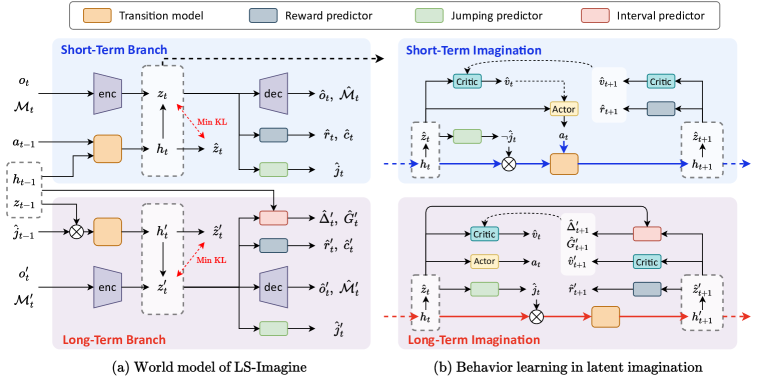
Figure 3: The overall architecture of the world model and the behavior learning process.

In LS-Imagine, the state transition model includes both short-term and long-term branches. The short-term transition model integrates the previous deterministic recurrent state $h_{t-1}$, stochastic state $z_{t-1}$, and action $a_{t-1}$ to adopt the single-step transition. In contrast, the long-term transition model simulates multiple-step transitions toward the target. At time step $t$, we feed the recurrent state $h_{t}$, the observation $o_{t}$, and the affordance map $\mathcal{M}_{t}$ into the encoder to obtain posterior state $z_{t}$. Notably, we also use the affordance map as an input of the encoder, which serves as the goal-conditioned prior guidance to the agent. Meanwhile, the prediction of prior state $\hat{z}_{t}$ does not involve the current observation or affordance map, relying only on information from history. We use $(h_{t},z_{t})$ to reconstruct the visual observation $\hat{o}_{t}$ and the affordance map $\hat{\mathcal{M}}_{t}$, and predict the reward $\hat{r}_{t}$, episode continuation flag $\hat{c}_{t}$, and jumping flag $\hat{j}_{t}$. For states that have adopted a long-term state transition, we employ an interval predictor to estimate the expected number of steps $\hat{\Delta}_{t}^{\prime}$ required to transition from the pre-transition state $(h_{t-1},z_{t-1})$ to the post-transition state $({h}^{\prime}_{t},{z}^{\prime}_{t})$, as well as the expected cumulative reward $\hat{G}_{t}^{\prime}$ the agent might receive during this interval.

To train the world model, we interact with the environment to collect short-term tuples $\mathcal{D}_{t}=(o_{t},a_{t},r_{t},c_{t},\mathcal{M}_{t},j_{t},\Delta_{t},G_{t})$ and long-term tuples $\mathcal{D}^{\prime}_{t}=(o_{t}^{\prime},a_{t}^{\prime},{r}_{t}^{\prime},\mathcal{M}^{\prime}_{t},c_{t}^{\prime},j_{t}^{\prime},\Delta_{t}^{\prime},G_{t}^{\prime})$ using the current policy. More details for environment interaction and data collection can be found in Appendix B.1. During representation learning, we sample short-term tuples $\{\mathcal{D}_{t}\}_{t=1}^{T}$ and the long-term tuples following jumpy transitions $\{\mathcal{D}_{t}^{\prime}\}_{t\in\mathcal{T}}$ from the replay buffer $\mathcal{B}$, where $\mathcal{T}$ denotes the set of time steps at which long-term state transitions are required. The loss functions for each component of the short-term and long-term world model branch are as follows:

$$\begin{aligned} &\text{Short-term branch:}\quad\left\{\begin{aligned} \mathcal{L}_{\text{dyn}}&\doteq\max\left(1,\operatorname{KL}\left[\operatorname{sg}\left(q_{\phi}\left(z_{t}\mid h_{t},o_{t},\mathcal{M}_{t}\right)\right)\parallel p_{\phi}\left(z_{t}\mid h_{t}\right)\right]\right)\\ \mathcal{L}_{\text{enc}}&\doteq\max\left(1,\operatorname{KL}\left[q_{\phi}\left(z_{t}\mid h_{t},o_{t},\mathcal{M}_{t}\right)\parallel\operatorname{sg}\left(p_{\phi}\left(z_{t}\mid h_{t}\right)\right)\right]\right)\\ \mathcal{L}_{\text{dec}}&\doteq-\operatorname{ln}p_{\phi}\left(o_{t},\mathcal{M}_{t}\mid h_{t},z_{t}\right)\\ \mathcal{L}_{\text{pred}}&\doteq-\operatorname{ln}p_{\phi}\left({r}_{t},{c}_{t}\mid h_{t},z_{t}\right)-\operatorname{ln}p_{\phi}\left({j}_{t}\mid h_{t},z_{t}\right)\end{aligned}\right.\\ &\text{Long-term branch:}\quad\left\{\begin{aligned} \mathcal{L}^{\prime}_{\text{dyn}}&\doteq\max\left(1,\operatorname{KL}\left[\operatorname{sg}\left(q_{\phi}\left({z}^{\prime}_{t}\mid{h}^{\prime}_{t},o^{\prime}_{t},{\mathcal{M}}^{\prime}_{t}\right)\right)\parallel p_{\phi}\left({z}^{\prime}_{t}\mid{h}^{\prime}_{t}\right)\right]\right)\\ \mathcal{L}^{\prime}_{\text{enc}}&\doteq\max\left(1,\operatorname{KL}\left[q_{\phi}\left({z}^{\prime}_{t}\mid{h}^{\prime}_{t},o^{\prime}_{t},{\mathcal{M}}^{\prime}_{t}\right)\parallel\operatorname{sg}\left(p_{\phi}\left({z}^{\prime}_{t}\mid{h}^{\prime}_{t}\right)\right)\right]\right)\\ \mathcal{L}^{\prime}_{\text{dec}}&\doteq-\operatorname{ln}p_{\phi}\left(o^{\prime}_{t},{\mathcal{M}}^{\prime}_{t}\mid{h}^{\prime}_{t},{z}^{\prime}_{t}\right)\\ \mathcal{L}^{\prime}_{\text{pred}}&\doteq-\operatorname{ln}p_{\phi}({r}^{\prime}_{t},{c}^{\prime}_{t}\mid{h}^{\prime}_{t},{z}^{\prime}_{t})-\operatorname{ln}p_{\phi}({{j}}^{\prime}_{t}\mid{h}^{\prime}_{t},{z}^{\prime}_{t})\\ \mathcal{L}^{\prime}_{\text{int}}&\doteq-\operatorname{ln}p_{\phi}\left({\Delta}^{\prime}_{t},G_{t}^{\prime}\mid h_{t-1},z_{t-1},{h}^{\prime}_{t},{z}^{\prime}_{t}\right)\end{aligned}\right.\end{aligned}.$$ (6)

We can optimize the world model $\mathcal{W}_{\phi}$ by minimizing over replay buffer $\mathcal{B}$:

$$\mathcal{L}\doteq\mathbb{E}\Big{[} {\textstyle\sum_{\{\mathcal{D}_{t}\}_{t=1}^{T}}}\left(\beta_{\text{dyn}}\mathcal{L}_{\text{dyn}}+\beta_{\text{enc}}\mathcal{L}_{\text{enc}}+\beta_{\text{pred}}\left(\mathcal{L}_{\text{dec}}+\mathcal{L}_{\text{pred}}\right)\right)+$$ (7)

$$\beta_{\text{long}} {\textstyle\sum_{{\{\mathcal{D}}^{\prime}_{t}\}_{t\in\mathcal{T}}}}\left(\beta_{\text{dyn}}\mathcal{L}^{\prime}_{\text{dyn}}+\beta_{\text{enc}}\mathcal{L}^{\prime}_{\text{enc}}+\beta_{\text{pred}}\left(\mathcal{L}^{\prime}_{\text{dec}}+\mathcal{L}^{\prime}_{\text{pred}}+\mathcal{L}^{\prime}_{\text{int}}\right)\right)\Big{]}.$$

3.4 Behavior Learning over Mixed Long Short-Term Imaginations

As shown in Figure 3 (b), LS-Imagine employs the actor-critic algorithm to learn behavior on the latent state sequences predicted by the world model. The goal of the actor is to optimize the policy to maximize the discounted cumulative reward $R_{t}$, while the role of the critic is to estimate the discounted cumulative rewards using the current policy for each state:

$$\text{Actor:}\quad a_{t}\sim\pi_{\theta}\left(a_{t}\mid h_{t},\hat{z}_{t}\right),\quad\text{Critic:}\quad v_{\psi}\left(R_{t}\mid h_{t},\hat{z}_{t}\right).$$ (8)

Starting from the initial state encoded from the sampled observation and the affordance map, we dynamically select either the long-term transition model or the short-term transition model to predict subsequent states based on the jumping flag $\hat{j}_{t}$. For the long short-term imagination sequence $\{(h_{t},\hat{z}_{t},a_{t})\}_{t=1}^{L}$ with an imagination horizon of $L$, we predict reward sequence $\hat{r}_{1:L}$ and the continuation flag sequence $\hat{c}_{1:L}$ through the reward predictor.

For jumpy states predicted by long-term imagination, the interval predictor estimates the number of steps $\hat{\Delta}_{t}$ between it and the previous state, as well as the potential discounted cumulative reward $\hat{G}_{t}$ during this period. Specifically, for instant states from short-term imagination, we set $\hat{\Delta}_{t}=1$ and $\hat{G}_{t}=\hat{r}_{t}$. We employ a modified bootstrapped $\lambda$-returns that considers both long-term and short-term imaginations to calculate the discounted cumulative rewards for each state:

$$R_{t}^{\lambda}\doteq\left\{\begin{array}[]{ll}\hat{c}_{t}\{\hat{G}_{t+1}+\gamma^{\hat{\Delta}_{t+1}}\left[(1-\lambda)v_{\psi}(h_{t+1},\hat{z}_{t+1})+\lambda R_{t+1}^{\lambda}\right]\}&\text{if }t<L\\ v_{\psi}(h_{L},\hat{z}_{L})&\text{if }t=L\end{array}\right..$$ (9)

The critic uses the maximum likelihood loss to predict the distribution of the return estimates $R_{t}^{\lambda}$:

$$\mathcal{L}(\psi)\doteq-\sum_{t=1}^{L}\ln p_{\psi}\left(R_{t}^{\lambda}\mid h_{t},\hat{z}_{t}\right).$$ (10)

Following DreamerV3 (Hafner et al., 2023), we train the actor to maximize the return estimates $R_{t}^{\lambda}$. Notably, due to long-term imagination does not involve action, we do not optimize $a_{t}$ when long-term imagination is adopted. The loss of actor is formulated as:

$$\mathcal{L}(\theta)\doteq-\sum_{t=1}^{L}\text{sg}\left[\left(1-\hat{j}_{t}\right)\frac{R_{t}^{\lambda}-v_{\psi}(h_{t},\hat{z}_{t})}{\max(1,S)}\right]\log\pi_{\theta}(a_{t}\mid h_{t},\hat{z}_{t})+\eta\,\text{H}\left[\pi_{\theta}(a_{t}\mid h_{t},\hat{z}_{t})\right].$$ (11)

4 Experiments

4.1 Experimental Setups

Benchmark.

We explore LS-Imagine on challenging MineDojo (Fan et al., 2022) benchmark on top of the popular Minecraft game, which is a comprehensive simulation platform with various open-ended tasks. We use $5$ challenging tasks, i.e., harvest log in plains, harvest water with bucket, harvest sand, shear sheep, and mine iron ore. These tasks demand numerous steps to complete and present significant challenges for agent learning. Additionally, we adopt a binary reward that indicates whether the task was completed, along with the MineCLIP reward proposed in Fan et al. (2022).

Further details of the environmental setups are provided in Appendix A.

Compared methods.

We compare LS-Imagine with strong MineCraft agents, including

• DreamerV3 (Hafner et al., 2023): An MBRL approach that learns directly from the step-by-step imaginations of future latent states generated by the world model.

• VPT (Baker et al., 2022): A foundation model designed for Minecraft trained through behavior cloning, on a dataset consisting of $70{,}000$ hours of game playing collected from the Internet.

• STEVE-1 (Lifshitz et al., 2023): An instruction-following agent developed for Minecraft. The development process begins by training a goal-conditioned policy using the contractor dataset. This policy serves as the low-level controller. Subsequently, Steve-1 employs a language-labeled dataset to translate language instructions into specific goals. To evaluate its effectiveness, we assess Steve-1’s zero-shot performance on our tasks by supplying it with task instructions.

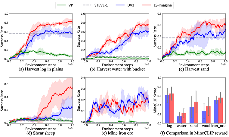
Figure 4: Performance comparison of LS-Imagine against existing approaches in MineDojo.

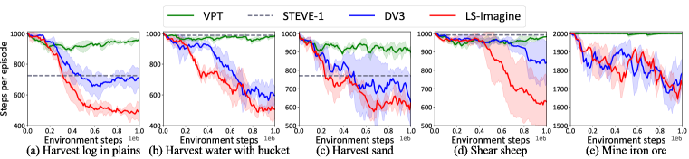
Figure 5: Number of steps per episode required to achieve success in MineDojo.

Implementation details.

We conduct our experiments on the MineDojo environment, where both visual observation and corresponding affordance maps are resized to $64\times 64$ pixels to serve as inputs to the model. To generate affordance maps accurately, we collect $2{,}000$ images from the environment using a random agent under the current task instruction and generate a discrete set of ($o_{t},I,\mathcal{M}_{o_{t},I}$), which are then used to finetune the multimodal U-Net for $200$ epochs. For tasks in the MineDojo benchmark, we train the agent for $1\times 10^{6}$ environment steps.

4.2 Main Comparison

We evaluate all the Minecraft agents in terms of success rate shown in Figure 4 and per-episode steps shown in Figure 5. We find that LS-Imagine significantly outperforms the compared models, particularly in scenarios where sparse targets are distributed in the task. In Figure 4 (f), we showcase the MineCLIP values achieved by LS-Imagine and DreamerV3. Specifically, a sliding window of length $16$ is used to compute the local MineCLIP values for each segment. The mean value is then calculated from all sliding windows. We can see that agents trained using our method achieve higher MineCLIP values within a single episode compared to DreamerV3. This suggests that LS-Imagine facilitates quicker detection of task-relevant visual targets in open-world environments.

Additionally, we present qualitative results in Figure 6(a). In the top row, we decode the latent states before and after the jumpy state transitions back to the pixel space. To better understand how affordance maps facilitate the jumpy state transitions and whether they can provide effective goal-conditioned guidance, the bottom rows visualize the affordance maps reconstructed from the latent states. These visualizations demonstrate that the proposed world model can adaptively determine when to utilize long-term imagination based on the current visual observation. Furthermore, the generated affordance maps align effectively with areas that are highly relevant to the final goal, thereby enabling the agent to perform more efficient policy exploration.

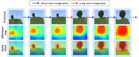
(a) Visualization of long short-term imaginations

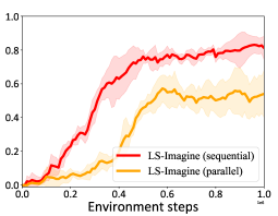
(b) Series vs. parallel connections

Figure 6: (a) Visualization of long short-term imaginations and (b) a further discussion on possible architecture designs of Series and Parallel connections of these two imagination pathways.

4.3 Model Analyses

Alternative pathways of mixed imaginations.

It is worth highlighting that the long short-term imagination is implemented sequentially. Alternatively, we could structure long- and short-term imagination pathways in parallel. Specifically, we first apply short-term imagination in a single sequence. Then, for all states predicted by this short-term imagination, if the jumping flag is True, we use the post-jumping state as the initial state to generate another sequence using short-term imagination. To evaluate the advantages of using sequential long short-term imagination, we conduct an experimental comparison between LS-Imagine (series) and LS-Imagine (parallel). Figure 6(b) shows that the LS-Imagine (series) outperforms LS-Imagine (parallel) by large margins. This implies that the parallel imagination sequences are independent of one another, meaning that the sequence starting with a post-jumping state does not guide the prior-jumping transitions.

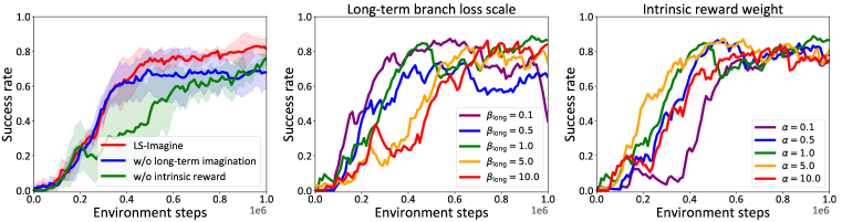
Figure 7: Results of ablation studies (Left) and hyperparameter analyses (Middle/Right).

Ablation studies.

We conduct the ablation studies to validate the effect of the affordance-driven intrinsic reward and long short-term imagination. Figure 7 (Left) presents corresponding results in the challenging MineDojo tasks. As shown by the blue curve, removing the long-term imagination of LS-Imagine leads to a performance decline, which indicates the necessity of introducing long-term imagination and switching between it and short-term imagination adaptively. For the model represented by the green curve, we do not employ affordance-driven intrinsic reward. It shows that the affordance-driven intrinsic reward also plays an important role during the early training state of agents. Additionally, unlike the MineCLIP reward being calculated based on a series of states, the affordance-driven intrinsic reward relies solely on a single independent state. This approach enables a more accurate estimation of the reward for the post-jumpy-transition state.

Hyperparameter sensitivity.

We conduct sensitivity analyses on two hyperparameters: the long-term branch loss scale $\beta_{\text{long}}$ and the intrinsic reward weight $\alpha$. As shown in Figure 7 (Middle), we observe that when $\beta_{\text{long}}$ for the long-term branch is too small or too large, it impedes the learning of long-term imagination, leading to a decline in performance. Moreover, as we can see from Figure 7 (Right), if the hyperparameter $\alpha$ for intrinsic reward is excessively small, it may result in insufficient guidance and inaccurate reward estimation for the post-jumpy-transition state.

5 Related Work

Visual MBRL.

Recently, learning control policies from images, i.e., visual RL has been used widely, whereas previous RL algorithms learn policies from low-dimensional states. Existing approaches can be grouped by the use of model-free (Laskin et al., 2020; Schwarzer et al., 2021; Stooke et al., 2021; Xiao et al., 2022; Parisi et al., 2022; Yarats et al., 2022; Zheng et al., 2023) or model-based (Hafner et al., 2019; 2020; 2021; Seo et al., 2022; Pan et al., 2022; Hafner et al., 2022; Mazzaglia et al., 2023; Micheli et al., 2023; Zhang et al., 2023; Ying et al., 2023; Hansen et al., 2024; Wang et al., 2024b) RL algorithms. Lee et al. (2024b) proposed predicting a temporally smoothed reward instead of the exact reward at a given timestep, particularly for long-horizon sparse-reward tasks. This approach helps alleviate the challenges associated with reward prediction. R2I (Samsami et al., 2024) introduced state space models (SSMs) within the world models of MBRL to improve both long-term memory and long-horizon credit assignment. Gumbsch et al. (2024) presented a fully self-supervised algorithm for constructing hierarchical world models, which learns a hierarchy of world models featuring discrete latent dynamics. MV-MWM (Seo et al., 2023) employs a multi-view masked autoencoder for representation learning and subsequently trains a world model based on the representations generated by the autoencoder. Unlike the aforementioned approaches, our work presents a long short-term world model architecture specifically designed for visual control in open-world environments.

Affordance maps for robot learning.

Our work is also related to the affordance map for robot learning, which is known as to utilize the affordance to facilitate robot learning (Mo et al., 2021; Jiang et al., 2021; Yarats et al., 2021; Mo et al., 2022; Geng et al., 2022; Xu et al., 2022a; Wang et al., 2022; Wu et al., 2022; Ha & Song, 2022; Xu et al., 2022b; Cheng et al., 2024; Lee et al., 2024a; Li et al., 2024b). Where2Explore (Ning et al., 2023) introduces a cross-category few-shot affordance learning framework that leverages the similarities in geometries across different categories. DualAfford (Zhao et al., 2023) learns collaborative actionable affordance for dual-gripper manipulation tasks over various 3D shapes. VoxPoser (Huang et al., 2023) unleashes the power of large language models and vision-language models for extracting affordances and constraints of real-world manipulation tasks, which are grounded in 3D perceptual space. VRB (Bahl et al., 2023) train a visual affordance model with videos of human interactions and deploy the model in real-world robotic tasks directly. However, our approach distinguishes itself by employing visual observation to generate affordance maps as guidance to mitigate the low exploration efficiency in open-world environments.

6 Conclusions and Limitations

In this paper, we presented a novel approach to overcoming the challenges of training visual reinforcement learning agents in high-dimensional open worlds. By extending the imagination horizon and leveraging a long short-term world model, our method facilitates efficient off-policy exploration across expansive state spaces. The incorporation of goal-conditioned jumpy state transitions and affordance maps allows agents to better grasp long-term value, enhancing their decision-making abilities. Our results demonstrate substantial improvements over existing state-of-the-art techniques in MineDojo, highlighting the potential of our approach for open-world reinforcement learning and inspiring future research in this domain.

Although our approach demonstrates significant potential and effectiveness, it also introduces complexity in model training, and its generalizability across diverse tasks remains to be fully explored.

Appendix

Appendix A Environment Details

As illustrated in Table 2, language description is employed for calculating the MineCLIP reward (Fan et al., 2022). Initial tools are the items provided in the inventory at the beginning of each episode. Initial mobs and distance specifies the types of mobs present at the start of each episode and their initial distance from the agent. Max steps refers to the maximum allowed steps per episode.

Table 2: Details of four tasks in MineDojo.

Task	Language description	Initial tools	Initial mobs and distance	Max steps
Harvest log in plains	“Cut a tree.”	–	–	1000
Harvest water with bucket	“Obtain water.”	bucket	–	1000
Harvest sand	“Obtain sand.”	–	–	1000
Shear sheep	“Obtain wool.”	shear	sheep, 15	1000
Mine iron ore	“Mine iron ore.”	stone pickaxe	–	2000

Appendix B Model Details

B.1 Environment Interaction and Data Collection

To train the world model in our LS-Imagine, we need to collect both short-term and long-term transition data through interactions with the environment. As shown in Figure 8, at each time step $t$, we interact with the environment following the current policy, corresponding to a short-term transition. The data sequence collected at each time step is denoted as $\mathcal{D}_{t}$, which includes: $\{o_{t},a_{t},r_{t},c_{t},\mathcal{M}_{t},j_{t},\Delta_{t},G_{t}\}$. For simplicity, we denote the data collected at a specific time step with the subscript $t$.

In this sequence, $a_{t}$ and $o_{t}$ represent the action taken during the interaction and the observation image returned by the environment, respectively. The continuation flag $c_{t}$ indicates whether further interaction is required after this step. We generate the affordance map $\mathcal{M}_{t}$ by feeding the observation image $o_{t}$ and the current task instruction $I$ into the multimodal U-Net. Based on the visual observation and the affordance map, we calculate the MineCLIP reward and the affordance-driven intrinsic reward $r_{t}^{i}$ using Eq. (1). The total reward is computed as a weighted sum of the environmental reward $r_{t}^{e}$, the MineCLIP reward, and the intrinsic reward, $r_{t}=r^{e}_{t}+r_{t}^{\text{MineCLIP}}+\alpha r^{i}_{t}$, where $\alpha$ is a hyperparameter. We also compute the jump probability $P_{\text{jump}}$ using Eq. (4) based on the affordance map to determine whether a distant target is present in the observation, indicating the need for a jumpy transition. The jump flag $j_{t}$ is determined by setting a threshold, which is the average of all previous jump probabilities plus the standard deviation. If $P_{\text{jump}}$ exceeds this threshold, the jump flag $j_{t}$ is True.

$\Delta_{t}$ and $G_{t}$ represent the number of steps between transitions and the cumulative discounted reward obtained during this period, respectively. For short-term transitions, where only one environmental step occurs, we set $\Delta_{t}=1$ and $G_{t}=r_{t}$.

If the jump flag is True, this indicates that the agent has observed a distant target, and a jumpy transition (i.e., a long-term transition) can be performed to transition to a state closer to the target. In this case, we need to collect the long-term transition data sequence $\mathcal{D}_{t}^{\prime}$, which includes: $\{o_{t}^{\prime},a_{t}^{\prime},r_{t}^{\prime},c_{t}^{\prime},\mathcal{M}_{t}^{\prime},j_{t}^{\prime},\Delta_{t}^{\prime},G_{t}^{\prime}\}$. Long-term transitions simulate the agent’s state at a future time after a sequence of exploration steps.

For the observation $o_{t}^{\prime}$, we crop the high-value regions from the original observation $o_{t-1}$ based on the affordance map $\mathcal{M}_{t-1}$ to simulate the image that the agent would observe after approaching the target. Similarly, we generate the affordance map $\mathcal{M}_{t}^{\prime}$ by feeding the observation $o_{t}^{\prime}$ and the task instruction $I$ into the multimodal U-Net. Based on the image and the affordance map, other data such as the rewards and flags are computed. Specifically, $\Delta_{t}^{\prime}$ and $G_{t}^{\prime}$ are used to record the number of steps between transitions and the cumulative discounted reward obtained during the long-term transition. They are estimated as follows: starting from time $t$, when the agent interacts with the environment and reaches a state where the level of exploration matches that of the post-jumpy-transition state (measured by the reward of the state), the number of steps since time $t$ is recorded as $\Delta_{t}^{\prime}$, and the cumulative reward during this period is recorded as $G_{t}^{\prime}$.

Figure 8: Environment interaction and data collection.

B.2 Framework of Multimodal U-Net

As described in Sec. 3.2.2, we train a multimodal U-Net to rapidly generate affordance maps based on observation images and task instructions. Our enhanced multimodal U-Net architecture, as illustrated in Figure 9, is based on Swin-Unet (Cao et al., 2022), a U-shaped encoder-decoder architecture built on Swin Transformer blocks. The enhanced multimodal U-Net consists of an encoder, a decoder, a bridge layer, and a text processing module. In the Swin-Unet-inspired structure, the basic unit is the Swin Transformer block. For the encoder, the input image is divided into non-overlapping patches of size $4\times 4$ to convert the input into a sequence of patch embeddings. Through this method, each patch has a feature dimension of $4\times 4\times 3=48$. The patch embeddings are then projected through a linear embedding layer (denoted as $C$), and the transformed patch tokens are passed through several Swin Transformer blocks and patch merging layers to produce hierarchical feature representations. The patch merging layers are responsible for downsampling and increasing the dimensionality, while the Swin Transformer blocks handle feature representation learning.

For the task instruction, the text description is processed through the text encoder of MineCLIP (Cao et al., 2022) to obtain text embeddings, which are integrated with the image features extracted at each layer of the encoder via the Text-Image Attention (TIA) module. The TIA module employs a multi-head attention mechanism to fuse image features (as keys and values) with text features (as queries) in a multi-scale attention-based fusion. The resulting fused text-image features are passed through the bridge layer and are subsequently combined with the corresponding features during the upsampling process in the decoder.

The decoder comprises Swin Transformer blocks and patch expanding layers. The extracted context features are combined through the bridge layer with the multi-scale text-image features from the encoder to compensate for the spatial information lost during downsampling and to integrate the text information. Unlike the patch merging layers, the patch expanding layers are specifically designed for upsampling. They reshape the adjacent feature maps by performing a $2\times$ upsampling of the resolution, expanding the feature maps into larger ones. Finally, a final patch expanding layer performs a $4\times$ upsampling to restore the resolution of the feature map to the input resolution $W\times H$ ), followed by a linear projection layer applied on the upsampled features to produce pixel-level affordance maps.

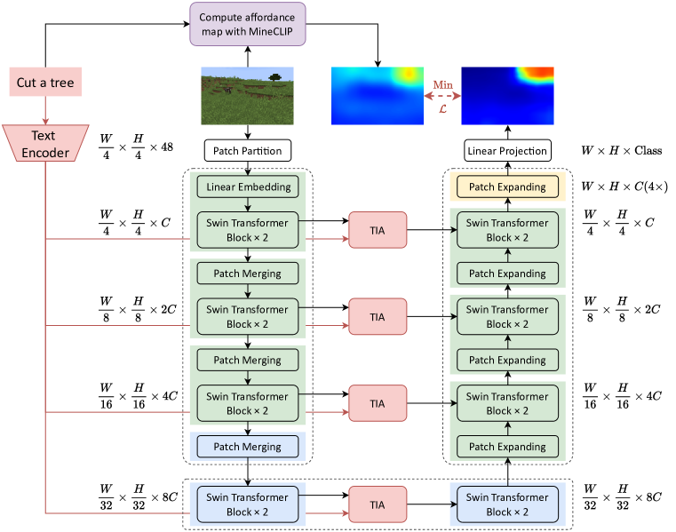
Figure 9: The architecture of multimodal U-Net.

Appendix C Additional Visualizations

As illustrated in Figure 10, we visualize the complete long short-term imagination sequences for the agent across various tasks. This visualization further demonstrates how the affordance map accurately identifies regions of high exploration potential in the image, and how the long short-term imagination approach provides reasonable and applicable guidance for the agent’s task execution. These qualitative results reinforce the effectiveness of our method in guiding the agent toward its goal with greater precision and efficiency.

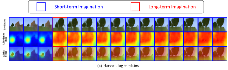
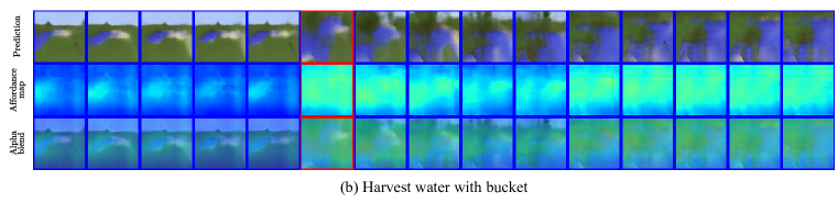
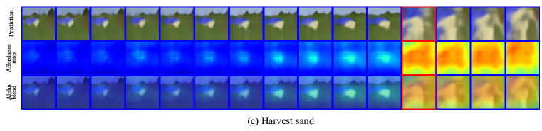
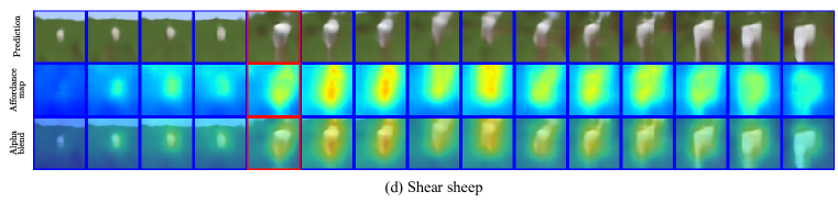
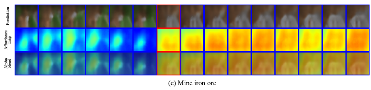
Figure 10: The visualization of the complete long short-term imagination sequences.

Appendix D Algorithm

The algorithm of LS-Imagine is illustrated in Alg. 1.

Algorithm 1 LS-Imagine.

1:Initialize parameters $\phi,\theta,\psi$.

2:Compute affordance map with MineCLIP. $\triangleright$ Affordance map generation

3:Train multimodal U-Net with annotated data. $\triangleright$ To enable real-time interaction with the affordance maps

4:Train the random agent and collect a replay buffer $\mathcal{B}$.

5:while not converged do

6:     Sample long short-term transitions from $\mathcal{B}$.$\triangleright$ Representation learning

7:     Update the world model $\phi$ using Eq. (7).

8:     Generate $(h_{t},{z}_{t},a_{t},j_{t})$ using $\pi_{\theta}$ and $\mathcal{W}_{\phi}$.$\triangleright$ Behavior learning

9:     for time step $i=t\cdots t+L$ do

10:         if jump flag $j_{i}$ then

11:              Generate $(h^{\prime},z^{\prime},a^{\prime},c^{\prime},j^{\prime},\Delta^{\prime},G^{\prime})$ using $\pi_{\theta}$ and long-term imagination of $\mathcal{W}_{\phi}$.

12:              Update $(h_{i+1},\hat{z}_{i+1},a_{i+1},\hat{c}_{i+1},\hat{j}_{i+1},\hat{\Delta}_{i+1},\hat{G}_{i+1})\leftarrow(h^{\prime},z^{\prime},a^{\prime},c^{\prime},j^{\prime},\Delta^{\prime},G^{\prime})$.

13:         else

14:              Generate $(\tilde{h}_{i+1},\tilde{z}_{i+1},\tilde{a}_{i+1},\tilde{r}_{i+1},\tilde{c}_{i+1},\tilde{j}_{i+1})$ using $\pi_{\theta}$ and short-term imagination of $\mathcal{W}_{\phi}$.

15:              Update $(h_{i+1},\hat{z}_{i+1},a_{i+1},\hat{r}_{i+1},\hat{c}_{i+1},\hat{j}_{i+1})\leftarrow(\tilde{h}_{i+1},\tilde{z}_{i+1},\tilde{a}_{i+1},\tilde{r}_{i+1},\tilde{c}_{i+1},\tilde{j}_{i+1})$.

16:         end if

17:     end for

18:     Calculate value estimate using Eq. (9).

19:     Optimize actor $\pi_{\theta}$ using Eq. (11) over $\{(h_{i+1},\hat{z}_{i+1},a_{i+1},\hat{r}_{i+1},\hat{c}_{i+1},\hat{j}_{i+1},\hat{\Delta}_{i+1},\hat{G}_{i+1})\}_{i=t}^{t+L}$.

20:     Optimize critic $v_{\psi}$ using Eq. (10) over $\{(h_{i+1},\hat{z}_{i+1},a_{i+1},\hat{r}_{i+1},\hat{c}_{i+1},\hat{j}_{i+1},\hat{\Delta}_{i+1},\hat{G}_{i+1})\}_{i=t}^{t+L}$.

21:     for time step $t=1\cdots T$ do $\triangleright$ Environment interaction

22:         Sample $a_{t}\sim v_{\psi}\left(R_{t}\mid h_{t},\hat{z}_{t}\right)$

23:         $r^{e}_{t},o_{t+1},c_{t}\leftarrow$ env.step($a_{t}$)

24:         Generate affordance map $\mathcal{M}_{t}$ with multimodal U-Net for each $o_{t}$.

25:         Calculate intrinsic reward $r^{i}_{t}$ and jump flag $j_{t}$ based on the affordance map.

26:         Collect short-term data $(o_{t},a_{t},r_{t},c_{t},\mathcal{M}_{t},j_{t},\Delta_{t},G_{t})$.

27:         if jumpy flag $j_{t}$ then

28:              Collect long-term data $(o_{t}^{\prime},a_{t}^{\prime},{{r}_{t}}^{\prime},c_{t}^{\prime},\mathcal{M}^{\prime}_{t},j_{t}^{\prime},\Delta_{t}^{\prime},G_{t}^{\prime})$ based on affordance map.

29:         end if

30:     end for

31:     Append long short-term transitions to $\mathcal{B}$.

32:end while

Appendix E Hyperparameters

The hyperparameters of LS-Imagine are shown in Table 3.

Table 3: Hyperparameters of LS-Imagine.

Name	Notation	Value
Affordance map generation
Sliding window size	—	$0.15\times 0.15$
Sliding steps	—	$9\times 9$
U-Net train epochs	—	$500$
U-Net initial learning rate	—	$5\times 10^{-4}$
U-Net learning rate decay epochs	—	$50$
U-Net learning rate decay rate	—	$0.10$
Text feature dimensions	—	$512$
General
Replay capacity	—	$1\times 10^{6}$
Batch size	$B$	$16$
Batch length	$T$	$32$
Train ratio	—	$16$
World Model
Intrinsic reward weight	$\alpha$	1
Deterministic latent dimensions	—	4096
Stochastic latent dimensions	—	32
Discrete latent classes	—	32
RSSM number of units	—	1024
World model learning rate	—	$1\times 10^{-4}$
Long-term branch loss scale	$\beta_{\text{long}}$	1
Reconstruction loss scale	$\beta_{\text{pred}}$	$1$
Dynamics loss scale	$\beta_{\text{dyn}}$	$1$
Representation loss scale	$\beta_{\text{rep}}$	$0.1$
Behavior Learning
Imagination horizon	$L$	15
Discount	$\gamma$	0.997
$\lambda$-target	$\lambda$	0.95
Actor learning rate	—	$3\cdot 10^{-5}$
Critic learning rate	—	$3\cdot 10^{-5}$

References

- Bahl et al. (2023) Shikhar Bahl, Russell Mendonca, Lili Chen, Unnat Jain, and Deepak Pathak. Affordances from human videos as a versatile representation for robotics. In CVPR, pp. 13778–13790, 2023.
- Baker et al. (2022) Bowen Baker, Ilge Akkaya, Peter Zhokov, Joost Huizinga, Jie Tang, Adrien Ecoffet, Brandon Houghton, Raul Sampedro, and Jeff Clune. Video pretraining (vpt): Learning to act by watching unlabeled online videos. In NeurIPS, 2022.
- Cao et al. (2022) Hu Cao, Yueyue Wang, Joy Chen, Dongsheng Jiang, Xiaopeng Zhang, Qi Tian, and Manning Wang. Swin-unet: Unet-like pure transformer for medical image segmentation. In ECCVW, 2022.
- Cheng et al. (2024) Guangran Cheng, Chuheng Zhang, Wenzhe Cai, Li Zhao, Changyin Sun, and Jiang Bian. Empowering large language models on robotic manipulation with affordance prompting. arXiv preprint arXiv:2404.11027, 2024.
- Fan et al. (2022) Linxi Fan, Guanzhi Wang, Yunfan Jiang, Ajay Mandlekar, Yuncong Yang, Haoyi Zhu, Andrew Tang, De-An Huang, Yuke Zhu, and Anima Anandkumar. Minedojo: Building open-ended embodied agents with internet-scale knowledge. In NeurIPS, volume 35, pp. 18343–18362, 2022.
- Geng et al. (2022) Yiran Geng, Boshi An, Haoran Geng, Yuanpei Chen, Yaodong Yang, and Hao Dong. End-to-end affordance learning for robotic manipulation. arXiv preprint arXiv:2209.12941, 2022.
- Gumbsch et al. (2024) Christian Gumbsch, Noor Sajid, Georg Martius, and Martin V. Butz. Learning hierarchical world models with adaptive temporal abstractions from discrete latent dynamics. In ICLR, 2024.
- Ha & Song (2022) Huy Ha and Shuran Song. Flingbot: The unreasonable effectiveness of dynamic manipulation for cloth unfolding. In CoRL, pp. 24–33, 2022.
- Hafner et al. (2019) Danijar Hafner, Timothy Lillicrap, Ian Fischer, Ruben Villegas, David Ha, Honglak Lee, and James Davidson. Learning latent dynamics for planning from pixels. In ICML, pp. 2555–2565, 2019.
- Hafner et al. (2020) Danijar Hafner, Timothy Lillicrap, Jimmy Ba, and Mohammad Norouzi. Dream to control: Learning behaviors by latent imagination. In ICLR, 2020.
- Hafner et al. (2021) Danijar Hafner, Timothy Lillicrap, Mohammad Norouzi, and Jimmy Ba. Mastering atari with discrete world models. In ICLR, 2021.
- Hafner et al. (2022) Danijar Hafner, Kuang-Huei Lee, Ian Fischer, and Pieter Abbeel. Deep hierarchical planning from pixels. arXiv preprint arXiv:2206.04114, 2022.
- Hafner et al. (2023) Danijar Hafner, Jurgis Pasukonis, Jimmy Ba, and Timothy Lillicrap. Mastering diverse domains through world models. arXiv preprint arXiv:2301.04104, 2023.
- Hansen et al. (2024) Nicklas Hansen, Hao Su, and Xiaolong Wang. Td-mpc2: Scalable, robust world models for continuous control. In ICLR, 2024.
- Huang et al. (2023) Wenlong Huang, Chen Wang, Ruohan Zhang, Yunzhu Li, Jiajun Wu, and Li Fei-Fei. Voxposer: Composable 3d value maps for robotic manipulation with language models. In CoRL, 2023.
- Jiang et al. (2021) Zhenyu Jiang, Yifeng Zhu, Maxwell Svetlik, Kuan Fang, and Yuke Zhu. Synergies between affordance and geometry: 6-dof grasp detection via implicit representations. Robotics: science and systems, 2021.
- Laskin et al. (2020) Michael Laskin, Aravind Srinivas, and Pieter Abbeel. Curl: Contrastive unsupervised representations for reinforcement learning. In ICML, pp. 5639–5650, 2020.
- Lee et al. (2024a) Olivia Y Lee, Annie Xie, Kuan Fang, Karl Pertsch, and Chelsea Finn. Affordance-guided reinforcement learning via visual prompting. arXiv preprint arXiv:2407.10341, 2024a.
- Lee et al. (2024b) Vint Lee, Pieter Abbeel, and Youngwoon Lee. Dreamsmooth: Improving model-based reinforcement learning via reward smoothing. In ICLR, 2024b.
- Li et al. (2024a) Hao Li, Xue Yang, Zhaokai Wang, Xizhou Zhu, Jie Zhou, Yu Qiao, Xiaogang Wang, Hongsheng Li, Lewei Lu, and Jifeng Dai. Auto mc-reward: Automated dense reward design with large language models for minecraft. In CVPR, pp. 16426–16435, 2024a.
- Li et al. (2024b) Xiaoqi Li, Mingxu Zhang, Yiran Geng, Haoran Geng, Yuxing Long, Yan Shen, Renrui Zhang, Jiaming Liu, and Hao Dong. Manipllm: Embodied multimodal large language model for object-centric robotic manipulation. In CVPR, pp. 18061–18070, 2024b.
- Lifshitz et al. (2023) Shalev Lifshitz, Keiran Paster, Harris Chan, Jimmy Ba, and Sheila McIlraith. Steve-1: A generative model for text-to-behavior in minecraft. In NeurIPS, 2023.
- Mazzaglia et al. (2023) Pietro Mazzaglia, Tim Verbelen, Bart Dhoedt, Alexandre Lacoste, and Sai Rajeswar. Choreographer: Learning and adapting skills in imagination. In ICLR, 2023.
- Micheli et al. (2023) Vincent Micheli, Eloi Alonso, and François Fleuret. Transformers are sample efficient world models. In ICLR, 2023.
- Mo et al. (2021) Kaichun Mo, Leonidas J Guibas, Mustafa Mukadam, Abhinav Gupta, and Shubham Tulsiani. Where2act: From pixels to actions for articulated 3d objects. In ICCV, pp. 6813–6823, 2021.
- Mo et al. (2022) Kaichun Mo, Yuzhe Qin, Fanbo Xiang, Hao Su, and Leonidas Guibas. O2o-afford: Annotation-free large-scale object-object affordance learning. In CoRL, pp. 1666–1677, 2022.
- Ning et al. (2023) Chuanruo Ning, Ruihai Wu, Haoran Lu, Kaichun Mo, and Hao Dong. Where2explore: Few-shot affordance learning for unseen novel categories of articulated objects. NeurIPS, 2023.
- Nottingham et al. (2023) Kolby Nottingham, Prithviraj Ammanabrolu, Alane Suhr, Yejin Choi, Hannaneh Hajishirzi, Sameer Singh, and Roy Fox. Do embodied agents dream of pixelated sheep: Embodied decision making using language guided world modelling. In ICML, pp. 26311–26325, 2023.
- Pan et al. (2022) Minting Pan, Xiangming Zhu, Yunbo Wang, and Xiaokang Yang. Iso-dream: Isolating and leveraging noncontrollable visual dynamics in world models. In NeurIPS, volume 35, pp. 23178–23191, 2022.
- Parisi et al. (2022) Simone Parisi, Aravind Rajeswaran, Senthil Purushwalkam, and Abhinav Gupta. The unsurprising effectiveness of pre-trained vision models for control. In ICML, pp. 17359–17371, 2022.
- Samsami et al. (2024) Mohammad Reza Samsami, Artem Zholus, Janarthanan Rajendran, and Sarath Chandar. Mastering memory tasks with world models. In ICLR, 2024.
- Schwarzer et al. (2021) Max Schwarzer, Nitarshan Rajkumar, Michael Noukhovitch, Ankesh Anand, Laurent Charlin, R Devon Hjelm, Philip Bachman, and Aaron C Courville. Pretraining representations for data-efficient reinforcement learning. In NeurIPS, volume 34, pp. 12686–12699, 2021.
- Seo et al. (2022) Younggyo Seo, Kimin Lee, Stephen L James, and Pieter Abbeel. Reinforcement learning with action-free pre-training from videos. In ICML, pp. 19561–19579, 2022.
- Seo et al. (2023) Younggyo Seo, Junsu Kim, Stephen James, Kimin Lee, Jinwoo Shin, and Pieter Abbeel. Multi-view masked world models for visual robotic manipulation. In ICML, pp. 30613–30632, 2023.
- Stooke et al. (2021) Adam Stooke, Kimin Lee, Pieter Abbeel, and Michael Laskin. Decoupling representation learning from reinforcement learning. In ICML, pp. 9870–9879, 2021.
- Wang et al. (2024a) Guanzhi Wang, Yuqi Xie, Yunfan Jiang, Ajay Mandlekar, Chaowei Xiao, Yuke Zhu, Linxi Fan, and Anima Anandkumar. Voyager: An open-ended embodied agent with large language models. TMLR, 2024a.
- Wang et al. (2024b) Qi Wang, Junming Yang, Yunbo Wang, Xin Jin, Wenjun Zeng, and Xiaokang Yang. Making offline rl online: Collaborative world models for offline visual reinforcement learning. In NeurIPS, 2024b.
- Wang et al. (2022) Yian Wang, Ruihai Wu, Kaichun Mo, Jiaqi Ke, Qingnan Fan, Leonidas J Guibas, and Hao Dong. Adaafford: Learning to adapt manipulation affordance for 3d articulated objects via few-shot interactions. In ECCV, pp. 90–107, 2022.
- Wang et al. (2023) Zihao Wang, Shaofei Cai, Guanzhou Chen, Anji Liu, Xiaojian Ma, and Yitao Liang. Describe, explain, plan and select: Interactive planning with large language models enables open-world multi-task agents. In NeurIPS, 2023.
- Wu et al. (2022) Ruihai Wu, Yan Zhao, Kaichun Mo, Zizheng Guo, Yian Wang, Tianhao Wu, Qingnan Fan, Xuelin Chen, Leonidas Guibas, and Hao Dong. Vat-mart: Learning visual action trajectory proposals for manipulating 3d articulated objects. ICLR, 2022.
- Xiao et al. (2022) Tete Xiao, Ilija Radosavovic, Trevor Darrell, and Jitendra Malik. Masked visual pre-training for motor control. arXiv preprint arXiv:2203.06173, 2022.
- Xu et al. (2022a) Chao Xu, Yixin Chen, He Wang, Song-Chun Zhu, Yixin Zhu, and Siyuan Huang. Partafford: Part-level affordance discovery from 3d objects. arXiv preprint arXiv:2202.13519, 2022a.
- Xu et al. (2022b) Zhenjia Xu, Zhanpeng He, and Shuran Song. Universal manipulation policy network for articulated objects. IEEE robotics and automation letters, 7(2):2447–2454, 2022b.
- Yarats et al. (2021) Denis Yarats, Ilya Kostrikov, and Rob Fergus. Image augmentation is all you need: Regularizing deep reinforcement learning from pixels. In ICLR, 2021.
- Yarats et al. (2022) Denis Yarats, Rob Fergus, Alessandro Lazaric, and Lerrel Pinto. Mastering visual continuous control: Improved data-augmented reinforcement learning. In ICLR, 2022.
- Ying et al. (2023) Chengyang Ying, Zhongkai Hao, Xinning Zhou, Hang Su, Songming Liu, Jialian Li, Dong Yan, and Jun Zhu. Reward informed dreamer for task generalization in reinforcement learning. arXiv preprint arXiv:2303.05092, 2023.
- Zhang et al. (2023) Wendong Zhang, Geng Chen, Xiangming Zhu, Siyu Gao, Yunbo Wang, and Xiaokang Yang. Predictive experience replay for continual visual control and forecasting. arXiv preprint arXiv:2303.06572, 2023.
- Zhao et al. (2023) Yan Zhao, Ruihai Wu, Zhehuan Chen, Yourong Zhang, Qingnan Fan, Kaichun Mo, and Hao Dong. Dualafford: Learning collaborative visual affordance for dual-gripper manipulation. ICLR, 2023.
- Zheng et al. (2023) Ruijie Zheng, Xiyao Wang, Yanchao Sun, Shuang Ma, Jieyu Zhao, Huazhe Xu, Hal Daumé III, and Furong Huang. Taco: Temporal latent action-driven contrastive loss for visual reinforcement learning. In NeurIPS, volume 36, 2023.