Testing gravity with the full-shape galaxy power spectrum: first constraints on scale-dependent modified gravity

Abstract

Since the discovery of the accelerated expansion of the Universe in 1998, modified gravity (MG) theories have attracted considerable attention as alternatives to dark energy (DE). While distinguishing the effects of MG from those of DE using cosmic background expansion alone is difficult, the large-scale structure is expected to differ significantly. Among the plethora of MG models, we are particularly interested in those that introduce a scale dependence in the growth of perturbations; specifically, theories that introduce fifth forces mediated by scalar fields with a finite range accessible to cosmological probes. This is the case with $f(R)$ gravity, which is widely regarded as the most studied model in cosmology. In this work, we utilize, for the first time, the full-shape power spectrum of galaxies to constrain scale-dependent modified gravity theories. By using BOSS DR12 dataset, along with a BBN prior on $\omega_{b}$ and a Planck 2018 prior on $n_{s}$, we obtain an upper bound of $|f_{R0}|<5.89\times 10^{-6}$ at 68% confidence level (c.l.) and $<1.53\times 10^{-5}$ at 95% c.l. for the Hu-Sawicki ($n=1$) model. We discuss that it is highly unlikely these constraints will be significantly improved by future galaxy spectroscopic catalogs, such as DESI and Euclid.

I Introduction

The discovery of the accelerated expansion of the Universe marked a new era in cosmology [1, 2]. Although the simplest explanation for this phenomenon is provided by a cosmological constant, several groups have dedicated considerable effort to search for alternative descriptions that may ultimately expand our understanding of nature. One possibility is that general relativity (GR) is not the correct theory for describing gravity on large scales [3, 4, 5, 6, 7]. Besides its impact over the background, homogenous and isotropic cosmology, if a modified gravity (MG) theory is responsible of the accelerated expansion of the universe, one would expect to find its signatures in the clustering of matter as well [8, 9, 10, 11].

GR is distinctive in that, in the absence of anisotropic stresses, such as in the late-time universe, both scalar potentials of the metric in the Newtonian gauge are equal. In MG theories, however, this is generally not the case [12]. Instead, the potential in the Poisson equation differs from the potential that sources the geodesic equation. Consequently, although the background evolution of the universe may be unable to distinguish between MG and dark energy (DE), the large-scale structure (LSS) is typically very different. In DE models, LSS behaves similarly to $\Lambda$CDM because DE does not cluster. In contrast, typical MG theories introduce a finite-range attractive “fifth-force” mediated by a scalar field with mass $m_{\phi}$. For finite masses, the force between particles separated by distances larger than $1/m_{\phi}$ is exponentially suppressed, meaning that on the largest cosmological scales, gravity behaves according to GR. Successful MG models, however, employ screening mechanisms [13, 14, 15, 16], which arise from non-linearities in the scalar field and drive the equations of motion back to those of GR. It is at intermediate scales, typically from several tens of megaparsecs upward, where cosmology can effectively search for modifications to gravity.

In the galaxy power spectrum, the signature will appear above comoving wavenumbers $k\gtrsim k_{\text{MG}}(a)\equiv am_{\phi}(a)$, where $a$ is the scale factor of the Universe. Notice that the mass is dynamical, as it generally depends on environmental factors such as the local density or the local gravitational strength (e.g. [14]). In a cosmological context, this is reflected in its dependence on the scale factor $a$. For some models, the mass either vanishes or is too small, such that the scale of onset of MG is even larger than the horizon. Such theories produce linear growth of density fluctuations that can be considered scale-independent for practical purposes. On the other hand, we refer to theories as scale-dependent when $k_{\text{MG}}$ lies within the range accessible to cosmological probes. Since the “new” force is attractive and scale dependent, the power spectrum is enhanced above $k_{\text{MG}}$ in comparison to that in GR. This is the signature one would expect to observe at first glance, and use to constrain possible deviations from GR.

In this work we deal with the specific case of $f(R)$ gravity [17, 18], that modifies the Einstein-Hilbert action by adding an arbitrary function of the Ricci scalar to its Lagrangian density, $R\rightarrow R+f(R)$. At the linear level in cosmological perturbation theory (PT), the gravitational strength modifies the evolution of density fluctuation, such that the linear growth function equation takes the following form

$$\ddot{D}_{+}(k,t)+2H\dot{D}_{+}$$

$$\quad-\frac{3}{2}\Omega_{m}(a)H^{2}\left(1+\frac{2\beta^{2}k^{2}}{k^{2}+k^{2}_{\text{MG}}(a)}\right)D_{+}=0,$$ (1)

with $2\beta^{2}=1/3$. We are interested in theories where $am_{\phi}(a)$ grows as we back in time, since these reduce to GR in the early universe, and only affects the late times when the acceleration of the universe takes places. We notice from Eq. I that the linear growth carries a $k$ dependence as a consequence of the (finite) mass of the scalar field that was introduced into the theory.

The most studied $f(R)$ theory is the Hu-Sawicky (HS) gravity [19], with $f(R)\approx\text{constant}-f_{R0}\bar{R}^{n+1}/R^{n}/n$ a valid approximation in a cosmological scenario. Here, $\bar{R}$ is nowadays value of the Ricci scalar evaluated at the background evolution, and $f_{R0}$ the derivative of $f(R)$ with respecte to $R$ evaluated today. The mass of the associated scalar field is given by

$$m_{\phi}(a) =\sqrt{\frac{3H_{0}^{2}}{2|f_{R0}|}}\frac{(\Omega_{m}a^{-3}+4(1-\Omega_{m}))^{(2+n)/2}}{(4-3\Omega_{m})^{n/2}},$$ (2)

with $H_{0}$ the Hubble constant and $\Omega_{m}$ the matter abundance at present time.

In Fig. 1 we show the onset scale of MG, given by $k_{\text{MG}}$, as a function of the redshift for the HS model. We choose different parameters $n=0.1,1.0,2.0$ with $f_{R0}=-10^{-5}$ fixed (top panel), and $f_{R0}=-10^{4},-10^{5},-10^{6}$, with $n=1$ fixed (bottom panel). In all cases the mass $m_{\phi}(a)$ decays with time. Although a minima in $k_{\text{MG}}(a)$ appear because of the scale factor $a$ that convert physical to comoving wavenumbers. The vertical lines serve to mark the redshift bins $z_{1}=0.38$ and $z_{3}=0.61$ of the Baryon Oscillation Spectroscopic Survey (BOSS) of the SDSS-III [20, 21]. Notice that in regions below $k_{\text{MG}}$, the LSS is insensitive to the MG effects. Hence, this plot suggests that the redshifts covered by BOSS are idoneous to test HS model with parameter $n\sim 1$. In the bottom panel we further show the horizontal (dashed) line that correspond to $k=0.2\,h\,\text{Mpc}^{-1}$, which marks the onset of the breakdown of PT. In this work we will fit BOSS data using the HS model, in part for the above mentioned reason, but also because there are several N-body state-of-the-art simulations (in particular the MG-GLAM simulations [22, 23]), that we already have used to test our PT methodology in Ref. [24].

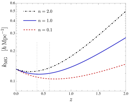
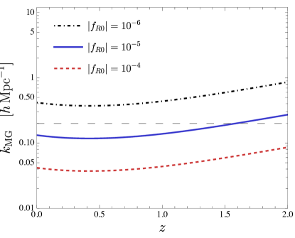
Figure 1: Onset scale of MG, $k_{\text{MG}}=am_{\phi}(a)$, as a function of redshift $z$ for the $f(R)$ HS model. Top panel: we show curves for parameters $n=0.1,1.0,2.0$ with $f_{R0}=-10^{-5}$ fixed. The vertical lines serve to mark the redshift bins $z_{1}=0.38$ and $z_{3}=0.61$ of BOSS. Bottom panel: $f_{R0}=-10^{4},-10^{5},-10^{6}$, with $n=1$. We further depict the scale $k=0.2\,h\,\text{Mpc}^{-1}$ (horizontal dashed line), roughly marking the failure of PT.

The rest of this work is organized as follows. In Sect. II we give a brief review of the PT scheme we use for our analysis. Section III presents the data we use. The main results of this work are presented in Sect. IV and further discussed In Sect. V. Finally, we present our conclusions in Sect. VI.

II Theoretical model

In this section, we provide a brief overview of the theory and code used for fitting the BOSS galaxy power spectrum. For more comprehensive details, see Ref. [24]. We utilize the PT for LSS formation, which has been developed for over more than two decades [25, 26, 27, 28, 29, 30, 31, 32], and by now has been largely applied to BOSS data sets; see Refs. [33, 34, 35, 36, 37], among many others. However, most of this work has been devoted to scenarios close to $\Lambda$CDM, employing the so-called Einstein-de Sitter (EdS) approximation that assumes $f(t)=\Omega_{m}^{1/2}(t)$, where $f(t)$ is the scale independent growth rate obtained from Eq. (I) without the effects of MG. In this work, we go beyond EdS and utilize the PT developed in [38, 39], based on works by other several authors [40, 41, 42, 43, 44, 45, 46, 47, 48, 49, 50, 51, 52, 53, 54]. While this theory is comprehensive, its practical application is limited, as the numerical implementation is highly time-consuming, making parameter space exploration infeasible. Therefore, we employ the fk-PT approximation [55, 56, 24], that keeps the scale-dependence in the growth factors, arising from the fact that, at linear order in PT, the velocity divergence and the density fluctuation of matter fields are not equal, but

$$\theta^{(1)}({\text{\bf k}},t)=\frac{f(k,t)}{f_{0}(t)}\delta^{(1)}({\text{\bf k}},t),$$ (3)

where the scale-dependent growth rate is

$$f({\text{\bf k}},t)\equiv\frac{d\log D_{+}(k,t)}{d\log a(t)}$$ (4)

and $f_{0}(t)=f({\text{\bf k}}=0,t)$ is the growth rate at the largest scales. Because the growth rate is k-dependent, the linear power spectra of the matter velocity and density fields are not equal, but they become related by

$$P_{\delta\theta}^{L}(k) =\frac{f(k)}{f_{0}}P_{\delta\delta}^{L}(k),$$ (5)

$$P_{\theta\theta}^{L}(k) =\left(\frac{f(k)}{f_{0}}\right)^{2}P_{\delta\delta}^{L}(k).$$ (6)

The one-loop redshift ($s$) space galaxy power spectrum is given by

$$P_{s}(k,\mu)=P_{s}^{\text{PT}}(k,\mu)+P_{s}^{\text{EFT}}(k,\mu)+P_{s}^{\text{shot}}(k,\mu),$$ (7)

where $\mu$ is the cosine of the angle between the line of sight direction and the wave vector k.

The pure perturbative term is given by

$$P_{s}^{\text{PT}}(k,\mu) =P_{\delta\delta}(k)+2f_{0}\mu^{2}P_{\delta\theta}(k)+f_{0}^{2}\mu^{4}P_{\theta\theta}(k)$$

$$+A^{\text{TNS}}(k,\mu)+D(k,\mu),$$ (8)

where the one-loop real space power spectra $P_{\delta\delta}$, $P_{\delta\theta}$, and $P_{\theta\theta}$ are the standard 2-point correlators of [60], and are displayed in Eqs. (3.74)-(3.76) of [24]. The functions $A^{\text{TNS}}$, defined in [61], and $D(k,\mu)$ are given by Eqs. (3.51) and (3.53) of [24].

We further add EFT counterterms of the form

$$P_{s}^{\text{EFT}}(k,\mu)=\big{(}\alpha_{0}+\alpha_{2}\mu^{2}+\cdots\big{)}k^{2}P_{L}(k),$$ (9)

accounting the backreaction from the unmodeled small scales—out of the reach of PT—over the large scales. The shot noise term is

$$P_{s}^{\text{shot}}(k,\mu)=\alpha_{0}^{\text{shot}}+(k\mu)^{2}\alpha^{\text{shot}}_{2}.$$ (10)

The biasing scheme differs slightly from that of $\Lambda$CDM, and is presented in [39]. Indeed, for scale-dependent MG, this scheme is not complete at any order in PT, but higher derivatives operators enter into the theory (see also [62]). However, we exclude these terms because they become degenerate with the EFT counterterms.

The final step is to model the spread and degradation of the BAO oscillations caused by large-scale bulk flows. To achieve this, we employ IR-resummations, as outlined in Refs. [63, 31]. The details of our implementation, closely following Refs. [64, 33], are presented in Sect. 3.6 of [24]. This approach allows us to compute the final expression for the power spectrum, $P_{s}^{\text{IR}}(k,\mu)$. For fitting the data, we use the multipoles from the equation

$$P_{\ell}(k)=\frac{2\ell+1}{2}\int_{-1}^{1}d\mu\,P_{s}^{\text{IR}}(k,\mu)\mathcal{L}_{\ell}(\mu),$$ (11)

where $\mathcal{L}_{\ell}$ is the Legendre polynomial of degree $\ell$.

All the one-loop corrections in Eq. (11) is computed in a fraction of a second using the code fkpt. The code receives as input the $\Lambda$CDM linear power spectrum and cosmological parameters, including those of GR. It then rescales this linear input with the use of the growth functions to generate the MG linear power spectrum

$$P_{L}^{\text{GR}}(k,z)=\left(\frac{D_{+}^{\text{GR}}(k,z)}{D_{+}^{\text{{\hbox{\Lambda}}CDM}}(k,z_{0})}\right)^{2}P_{L}^{\text{{\hbox{\Lambda}}CDM}}(k,z_{0}).$$ (12)

This equation holds for models that modify gravity only at high redshifts. In the case of HS $f(R)$ gravity, we have demonstrated that it is valid to an excellent approximation when compared to results obtained using the hi_class code [65]. For models where this is not true, one can use directly the MG power spectrum computed with a different code.

III Data

The BOSS survey collected spectroscopic redshifts for 1,198,006 galaxies through the SDSS multi-fiber spectrographs and multi-color imaging [21]. The BOSS-DR12 dataset spans redshifts from 0.2 to 0.75 over an effective area of 9,329 $\text{deg}^{2}$ and volume of $18.7\,\text{Gpc}^{3}$. These selections are organized into bins with effective redshifts at $z_{1}=0.38$, $z_{2}=0.51$, and $z_{3}=0.61$. For our study, we focus solely on the two non-overlapping bins, $z_{1}$ and $z_{3}$. Additionally, each redshift bin is divided into two sub-groups based on the galactic hemisphere in which the galaxies were observed, labeled as the “North Galactic Cap” (NGC) and “South Galactic Cap” (SGC).

We use the products provided in [66]. These include data vectors and window functions for the BOSS DR12 catalogue [67, 68], as well as the covariance matrices obtained from the MultiDark-Patchy mocks [69]. We refer the reader to Ref. [66] for further details

Parameter	Prior
$\quad|f_{R0}|$	$\mathcal{U}(0,0.1)$
$\quad\omega_{\text{cdm}}$	$\mathcal{U}(0.05,0.2)$
$\quad h$	$\mathcal{U}(0.4,0.9)$
$\quad\ln(10^{10}A_{s})$	$\mathcal{U}(2.0,4.0)$
$\quad\omega_{\text{b}}$	$\quad\mathcal{N}(0.02230,0.00038^{2})\,$
$\quad n_{s}$	$\quad\mathcal{N}(0.9649,0.0042^{2})\,$
$\quad b_{1}$	$\mathcal{U}(0.01,10)$
$\quad b_{2}$	$\mathcal{U}(-10,10)$
$\quad b_{s^{2}}$	$\quad\mathcal{N}(-4/7(b_{1}-1),0.05^{2})\,$
$\quad\alpha_{0}$	$\mathcal{N}(0,20^{2})$
$\quad\alpha_{2}$	$\mathcal{N}(0,20^{2})$
$\quad\alpha_{0}^{\text{shot}}$	Uninformative
$\quad\alpha_{2}^{\text{shot}}$	Uninformative

Table 1: Parameters and their priors. $\mathcal{N}(\mu,\sigma^{2})$ denotes a Gaussian prior with median $\mu$ and variance $\sigma^{2}$, while $\mathcal{U}(a,b)$ is uniform prior over the interval $(a,b)$. $b_{3nl}$ is fixed to its co-evolution value.

IV Results

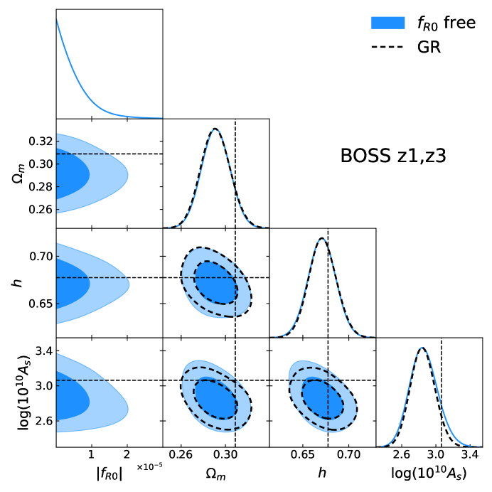
Figure 2: Corner plots for BOSS $z_{1}$ and $z_{3}$ constraints on the HS $f(R)$ gravity (blue) and GR (black dashed). We show the 68% and 95% contours, as well as the marginalized 1-dimensional distributions. The horizontal and vertical lines denote the best-fit values found by Planck 2018 [70].

In this section we confront the $f(R)$ HS ($n=1$) model with the BOSS data. To do this we run Monte Carlo Markov Chains (MCMC) using the codes CLASS [71], fkpt and the sampler emcee [72], which implements the affine-invariant ensemble sampler method [73]. We analyze the chains with the Python package GetDist [74], that we use also to plot our results.

The free parameters in our analysis include the amplitude of primordial scalar fluctuations $\log(10^{10}A_{s})$, the physical density of cold-dark matter $\omega_{c}$, the reduced Hubble constant $h$ and the MG parameter $f_{R0}$. Additionally, we impose a Gaussian prior on the spectral index $n_{s}$ based on Planck results [70], as well as a Big Bang Nucleosynthesis (BBN) Gausian prior for the baryon density $\omega_{b}$ [75, 76]. The neutrino mass is kept fixed at $\sum m_{\nu}=0.06\,\text{eV}$. We further utilize a set of nuisance parameters for each redshift bin and each galactic cap. These are the biases $b_{1}$, $b_{2}$ and $b_{s}$, the EFT counterterms $\alpha_{0}$, $\alpha_{2}$, and the shot noise parameters $\alpha_{0}^{\text{shot}}$ and $\alpha_{2}^{\text{shot}}$.

We analytically marginalize over EFT and noise parameters, which are linear in the power spectrum (before IR-resummations); see, e.g. Sect. 3.4 of [34]. Hence, we never fit them. That is, in total we vary 18 parameters, including both nuisance and cosmological. A summary of these parameters and their priors is provided in Table 1.

The pipeline outlined here was validated in [24] with the use of the $\Lambda$CDM NSeries mocks [21] and the $f(R)$ MG-GLAM simulation. In that study, we employed co-evolution theory for biases $b_{s}$ and $b_{3nl}$. However, we give a small liberty to the tidal bias around its coevolution value, while the third-order non-local bias remains fixed to $b_{3nl}=32/315(b_{1}-1)$ [77, 78, 79].

Since we are neglecting the nonlinearities responsible for producing the screening effect—that have been shown to be accurately handled by the EFT counterterms in [24]—our analysis is limited to a moderate maximum wavenumber of $k_{\text{max}}=0.17\,h\,\text{Mpc}^{-1}$. Further, in [24], we found this choice to be optimal for our study. The minimum wavenumber is $k_{\text{min}}=0.02\,h\,\text{Mpc}^{-1}$.

Our preliminary results indicate that leaving the EFT counterterms uninformative makes it infeasible to place meaningful constraints on $f_{R0}$, likely due to the lack of sufficient information to break parameter degeneracies. However, using very broad uniform priors (without analytical marginalization) does yield viable results. Therefore, we adopt Gaussuan priors with standard deviation $\sigma=20\,h^{-1}\text{Mpc}$ for the EFT parameters.

We present our results for the HS and GR models in Fig. 2 and Table 2. Notably, there are no significant degeneracies between $f_{R0}$ and the other cosmological parameters. This is very likely due to the scale-dependence of the gravitational strength. In scenarios where the large scales are impacted, as seen in the nDGP model in [58], degeneracies tend to be very pronounced. The absence of such degeneracies in our case suggests that we do not encounter additional projection effects than those present in the $\Lambda$CDM model [80, 81, 37] (also known as prior volume effects), which may arise when too many parameters control the overall amplitude of the power spectrum ($\Omega_{m}$, $h$, $A_{s}$, $b_{1}$, and $n_{s}$ to some extent). In contrast, $f_{R0}$ is a parameter that influences directly, and uniquely, the shape of the power spectrum at scales above $k_{\text{MG}}$.

At 1 and 2$\sigma$ we obtain the following constraints for $|f_{R_{0}}|$ in the HS, $n=1$ model are

$$|f_{R0}| <5.89\times 10^{-6}\qquad(68\%\,\,\text{c.l.}),$$ (13)

$$|f_{R0}| <1.53\times 10^{-5}\qquad(95\%\,\,\text{c.l.}).$$ (14)

In the next section, we will discuss why it is highly unlikely that these constraints can be significantly improved using the power spectrum from galaxy surveys. We will also compare our result with others in the literature.

Parameter $f_{R0}$ free GR $h$ $0.671\pm 0.014$ $0.671\pm 0.014$ $\Omega_{m}$ $0.291\pm 0.012$ $0.291\pm 0.013$ $f_{R0}$ $<5.89\times 10^{-6}$ $--$ $\log(10^{10}A_{s})$ $2.86^{+0.13}_{-0.17}$ $2.85\pm 0.14$ $b_{1}$ $2.19^{+0.19}_{-0.16}$ $2.19^{+0.17}_{-0.14}$

Table 2: 1-dimensional BOSS $z_{1}$ and $z_{3}$ constraints for the HS $f(R)$ gravity and GR. We show the mean of the posterior distributions with the 0.68 confidence level intervals.

V Discussions and prospects for future surveys

Nowadays, the most powerful tool to test the galaxy power spectrum from spectroscopic surveys is the full-shape technique given by PT. However, the scales reached in such theory is limited, below $k\sim 0.20\,h\,\text{Mpc}^{-1}$. In Fig.1 we showed such scales to give us a sense of the limits of our method. In the bottom panel of that figure, the horizontal dashed lines show this PT maximum scale. We notice that it lies well below the $k_{\text{MG}}$ for $|f_{R0}|=10^{-6}$, which means the upper bounds for $f_{R0}$ imposed by BOSS are indeed at the edge of what can be obtained with PT. The situation is even more critical since our approach assumes that the screening of the fifth force can be absorbed by EFT counterterms, forcing us to maintain our analysis below $k=0.17\,h\text{Mpc}^{-1}$. However, is possible that different techniques to treat screenings, as the one presented in [82], can reach a bit higher wavenumbers and then obtain a slightly tighter constraints.

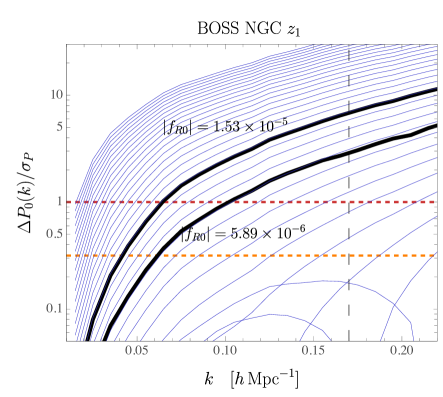
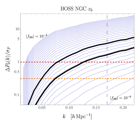
Figure 3: Signal to noise given. The lower vertical line (orange-dashed) shows the S/N rescaled with a factor $\sqrt{10}$, roughly representing a volume 10 times that of BOSS.

To elaborate more on this idea, Fig.3 presents plots illustrating the signal-to-noise ratio (S/N), as given by the difference in the monopole of the power spectrum, $\Delta P_{\ell=0}=P_{0}^{\text{MG}}-P_{0}^{\text{MG}}$, divided by the errors $\sigma_{P}$ obtained from the MultiDark-Patchy mocks. We show the $z_{1}$ (left panel) and $z_{3}$ (right panel) NGC samples, from top to bottom the blue thin lines show models with MG parameters from $f_{R0}=-10^{-3}$ to $-10^{-6}$ spaced in logarithmic intervals. The solid thick black lines show our constraints to 1 and $2\sigma$ given in Eqs. (13) and (14). The red dashed horizontal line indicates the S/N $=1$ threshold, which helps visualize which models can be distinguished, in the best-case scenario, using the BOSS DR12 dataset. Due to mode-coupling in non-linear theory, there can be small MG signatures even below $k_{\text{MG}}$. However, these are too small, such that even with a considerable rescaling of the effective surveyed volumes, the errors remains sufficiently large and no significant improvements are expected: the $1\sigma$ constraints will lie well above $|f_{R0}|=10^{-6}$. This is shown with the orange dashed horizontal lines in both panels, where the effective volume of the surveys is multiplied by a factor of 10. This analysis shows, first, that the limits we obtain for $|f_{R0}|$ are expected and reasonable. Second, it suggests that significantly improving these constraints is unlikely with the use of the full-shape technique alone in galaxy counts.

Finally, our constraints should be contrasted with those obtained using other methods. Currently, the most restrictive upper limit in the HS model is an impressive $|f_{R0}|<10^{-8}$, obtained from astrophysical scales [83], exceeding by far any limit imposed by cosmological probes. The tightest cosmological constraint in the HS model comes from a (very) recent joint analysis of weak-lensing mass-calibrated South Pole Telescope clusters and Planck 2018 data, yielding $|f_{R0}|<10^{-5.32}=4.79\times 10^{-6}$ [84]. Another recent cluster abundance analysis, conducted by eROSITA alone, provides a weaker constraint of $|f_{R0}|<10^{-4.12}=7.59\times 10^{-5}$ [85]. From LSS observations, the most stringent limit is given by weak lensing peak statistics from CFHTLenS [86], which yields an upper bound of $|f_{R0}|<10^{-4.82}=1.51\times 10^{-5}$, closely matching our result. But by including CMB priors on $\Omega_{m}$ and $A_{s}$, the authors achieve significantly tighter constraints, falling below $10^{-5}$.

VI Conclusions

In this work, we have confronted the HS $f(R)$ model using LSS data from the BOSS DR12 of the SDSS-III survey. We employed a full-shape analysis to constrain the $|f_{R0}|$ parameter. One of the challenges in such analysis is that using the standard EdS kernels in PT is unreliable. To address this, we utilized the fk-PT method developed in recent papers. Although this approach is not fully complete and employs a simplified version of the full kernels, it has proven to be an excellent approximation in $f(R)$ gravity. The pipeline we used here was recently validated through simulations, with mocks designed for both MG and the $\Lambda$CDM model.

By adding a BBN prior on $\omega_{b}$ and a Planck 2018 prior on $n_{s}$, we placed an upper bound of $|f_{R0}|<1.53\times 10^{-5}$ at 95 % confidence level. This result represents the first constraint on scale-dependent MG using the full-shape galaxy power spectrum.

An interesting aspect of our results is that introducing the parameter $|f_{R0}|$ does not seem to affect the other cosmological parameters. We believe this occurs because the MG signature does not significantly alter the large-scale power spectrum and its overall amplitude. In contrast, what we refer to in this work as scale-independent MG theories, such as DGP, introduces new parameters that strongly influence the overall power spectrum as much as other cosmological parameters, such as $A_{s}$, $h$, $\Omega_{m}$, as well as the linear bias $b_{1}$. On the other hand, $|f_{R0}|$ influences the shape of the power spectrum above a characteristic wavenumber $k_{\text{MG}}$, leaving the larger scales unaffected. This property does not seem to introduce additional projection effects beyond those already present in the $\Lambda$CDM model, leading us to believe that scale-dependent MG models are more easily constrained than scale-independent ones, despite the more intricate PT required.

We also discussed the expected results from future full-shape analyses of spectroscopic galaxy surveys, concluding that we do not foresee significant improvements due to the limitations of PT, as the results obtained with BOSS data are already at the edge of this limit. However, incorporating weak lensing data could provide additional constraints since the lensing potential depends directly on the sum of the two gravitational potentials in the metric (in Newtonian gauge). We will deal with such a joint analysis in future publications.

- [1] Supernova Cosmology Project collaboration, S. Perlmutter et al., Measurements of and from 42 High Redshift Supernovae, Astrophys. J. 517 (1999) 565–586, [astro-ph/9812133].
- [2] Supernova Search Team collaboration, A. G. Riess et al., Observational evidence from supernovae for an accelerating universe and a cosmological constant, Astron. J. 116 (1998) 1009–1038, [astro-ph/9805201].
- [3] C. Deffayet, G. R. Dvali and G. Gabadadze, Accelerated universe from gravity leaking to extra dimensions, Phys. Rev. D 65 (2002) 044023, [astro-ph/0105068].
- [4] S. Capozziello, Curvature quintessence, Int. J. Mod. Phys. D 11 (2002) 483–492, [gr-qc/0201033].
- [5] G. Dvali and M. S. Turner, Dark energy as a modification of the Friedmann equation, astro-ph/0301510.
- [6] S. M. Carroll, V. Duvvuri, M. Trodden and M. S. Turner, Is cosmic speed - up due to new gravitational physics?, Phys. Rev. D 70 (2004) 043528, [astro-ph/0306438].
- [7] T. P. Sotiriou and V. Faraoni, f(R) Theories Of Gravity, Rev. Mod. Phys. 82 (2010) 451–497, [0805.1726].
- [8] T. Clifton, P. G. Ferreira, A. Padilla and C. Skordis, Modified Gravity and Cosmology, Phys. Rept. 513 (2012) 1–189, [1106.2476].
- [9] K. Koyama, Cosmological Tests of Modified Gravity, Rept. Prog. Phys. 79 (2016) 046902, [1504.04623].
- [10] A. Joyce, L. Lombriser and F. Schmidt, Dark Energy Versus Modified Gravity, Ann. Rev. Nucl. Part. Sci. 66 (2016) 95–122, [1601.06133].
- [11] M. Ishak, Testing General Relativity in Cosmology, Living Rev. Rel. 22 (2019) 1, [1806.10122].
- [12] E. Bertschinger and P. Zukin, Distinguishing Modified Gravity from Dark Energy, Phys. Rev. D 78 (2008) 024015, [0801.2431].
- [13] A. I. Vainshtein, To the problem of nonvanishing gravitation mass, Phys. Lett. B 39 (1972) 393–394.
- [14] J. Khoury and A. Weltman, Chameleon cosmology, Phys. Rev. D 69 (2004) 044026, [astro-ph/0309411].
- [15] K. Hinterbichler and J. Khoury, Symmetron Fields: Screening Long-Range Forces Through Local Symmetry Restoration, Phys. Rev. Lett. 104 (2010) 231301, [1001.4525].
- [16] P. Brax, C. van de Bruck, A.-C. Davis and D. Shaw, The Dilaton and Modified Gravity, Phys. Rev. D 82 (2010) 063519, [1005.3735].
- [17] H. A. Buchdahl, Non-linear Lagrangians and cosmological theory, Mon. Not. Roy. Astron. Soc. 150 (1970) 1.
- [18] A. Starobinsky, A new type of isotropic cosmological models without singularity, Physics Letters B 91 (1980) 99–102.
- [19] W. Hu and I. Sawicki, Models of f(R) Cosmic Acceleration that Evade Solar-System Tests, Phys. Rev. D 76 (2007) 064004, [0705.1158].
- [20] BOSS collaboration, K. S. Dawson et al., The Baryon Oscillation Spectroscopic Survey of SDSS-III, Astron. J. 145 (2013) 10, [1208.0022].
- [21] BOSS collaboration, S. Alam et al., The clustering of galaxies in the completed SDSS-III Baryon Oscillation Spectroscopic Survey: cosmological analysis of the DR12 galaxy sample, Mon. Not. Roy. Astron. Soc. 470 (2017) 2617–2652, [1607.03155].
- [22] C. Hernández-Aguayo, C.-Z. Ruan, B. Li, C. Arnold, C. M. Baugh, A. Klypin et al., Fast full N-body simulations of generic modified gravity: derivative coupling models, JCAP 01 (2022) 048, [2110.00566].
- [23] C.-Z. Ruan, C. Hernández-Aguayo, B. Li, C. Arnold, C. M. Baugh, A. Klypin et al., Fast full N-body simulations of generic modified gravity: conformal coupling models, JCAP 05 (2022) 018, [2110.00328].
- [24] M. A. Rodriguez-Meza, A. Aviles, H. E. Noriega, C.-Z. Ruan, B. Li, M. Vargas-Magaña et al., fkPT: constraining scale-dependent modified gravity with the full-shape galaxy power spectrum, JCAP 03 (2024) 049, [2312.10510].
- [25] F. Bernardeau, S. Colombi, E. Gaztanaga and R. Scoccimarro, Large scale structure of the universe and cosmological perturbation theory, Phys. Rept. 367 (2002) 1–248, [astro-ph/0112551].
- [26] P. McDonald, Clustering of dark matter tracers: Renormalizing the bias parameters, Phys. Rev. D 74 (2006) 103512, [astro-ph/0609413].
- [27] P. McDonald and A. Roy, Clustering of dark matter tracers: generalizing bias for the coming era of precision LSS, JCAP 0908 (2009) 020, [0902.0991].
- [28] T. Matsubara, Resumming Cosmological Perturbations via the Lagrangian Picture: One-loop Results in Real Space and in Redshift Space, Phys. Rev. D 77 (2008) 063530, [0711.2521].
- [29] D. Baumann, A. Nicolis, L. Senatore and M. Zaldarriaga, Cosmological Non-Linearities as an Effective Fluid, JCAP 07 (2012) 051, [1004.2488].
- [30] J. Carlson, B. Reid and M. White, Convolution Lagrangian perturbation theory for biased tracers, Mon. Not. Roy. Astron. Soc. 429 (2013) 1674, [1209.0780].
- [31] Z. Vlah, M. White and A. Aviles, A Lagrangian effective field theory, JCAP 09 (2015) 014, [1506.05264].
- [32] S.-F. Chen, Z. Vlah and M. White, Consistent Modeling of Velocity Statistics and Redshift-Space Distortions in One-Loop Perturbation Theory, JCAP 07 (2020) 062, [2005.00523].
- [33] M. M. Ivanov, M. Simonović and M. Zaldarriaga, Cosmological Parameters from the BOSS Galaxy Power Spectrum, JCAP 05 (2020) 042, [1909.05277].
- [34] G. D’Amico, J. Gleyzes, N. Kokron, K. Markovic, L. Senatore, P. Zhang et al., The Cosmological Analysis of the SDSS/BOSS data from the Effective Field Theory of Large-Scale Structure, JCAP 05 (2020) 005, [1909.05271].
- [35] S.-F. Chen, Z. Vlah and M. White, A new analysis of galaxy 2-point functions in the BOSS survey, including full-shape information and post-reconstruction BAO, JCAP 02 (2022) 008, [2110.05530].
- [36] S.-F. Chen, M. M. Ivanov, O. H. E. Philcox and L. Wenzl, Suppression without Thawing: Constraining Structure Formation and Dark Energy with Galaxy Clustering, 2406.13388.
- [37] H. E. Noriega and A. Aviles, Unveiling Neutrino Masses: Insights from Robust (e)BOSS Data Analysis and Prospects for DESI and Beyond, 2407.06117.
- [38] A. Aviles and J. L. Cervantes-Cota, Lagrangian perturbation theory for modified gravity, Phys. Rev. D96 (2017) 123526, [1705.10719].
- [39] A. Aviles, G. Valogiannis, M. A. Rodriguez-Meza, J. L. Cervantes-Cota, B. Li and R. Bean, Redshift space power spectrum beyond Einstein-de Sitter kernels, JCAP 04 (2021) 039, [2012.05077].
- [40] K. Koyama, A. Taruya and T. Hiramatsu, Non-linear Evolution of Matter Power Spectrum in Modified Theory of Gravity, Phys. Rev. D 79 (2009) 123512, [0902.0618].
- [41] A. Taruya, K. Koyama, T. Hiramatsu and A. Oka, Beyond consistency test of gravity with redshift-space distortions at quasilinear scales, Phys. Rev. D 89 (2014) 043509, [1309.6783].
- [42] P. Brax and P. Valageas, Impact on the power spectrum of Screening in Modified Gravity Scenarios, Phys. Rev. D 88 (2013) 023527, [1305.5647].
- [43] E. Bellini and M. Zumalacarregui, Nonlinear evolution of the baryon acoustic oscillation scale in alternative theories of gravity, Phys. Rev. D 92 (2015) 063522, [1505.03839].
- [44] A. Taruya, T. Nishimichi, F. Bernardeau, T. Hiramatsu and K. Koyama, Regularized cosmological power spectrum and correlation function in modified gravity models, Phys. Rev. D 90 (2014) 123515, [1408.4232].
- [45] A. Taruya, Constructing perturbation theory kernels for large-scale structure in generalized cosmologies, Phys. Rev. D94 (2016) 023504, [1606.02168].
- [46] H. A. Winther, K. Koyama, M. Manera, B. S. Wright and G.-B. Zhao, COLA with scale-dependent growth: applications to screened modified gravity models, JCAP 08 (2017) 006, [1703.00879].
- [47] M. Fasiello and Z. Vlah, Screening in perturbative approaches to LSS, Phys. Lett. B 773 (2017) 236–241, [1704.07552].
- [48] B. Bose and K. Koyama, A Perturbative Approach to the Redshift Space Power Spectrum: Beyond the Standard Model, JCAP 08 (2016) 032, [1606.02520].
- [49] B. Bose and K. Koyama, A Perturbative Approach to the Redshift Space Correlation Function: Beyond the Standard Model, JCAP 08 (2017) 029, [1705.09181].
- [50] B. Bose, K. Koyama, M. Lewandowski, F. Vernizzi and H. A. Winther, Towards Precision Constraints on Gravity with the Effective Field Theory of Large-Scale Structure, JCAP 04 (2018) 063, [1802.01566].
- [51] G. Valogiannis and R. Bean, Convolution Lagrangian perturbation theory for biased tracers beyond general relativity, Phys. Rev. D 99 (2019) 063526, [1901.03763].
- [52] G. Valogiannis, R. Bean and A. Aviles, An accurate perturbative approach to redshift space clustering of biased tracers in modified gravity, JCAP 01 (2020) 055, [1909.05261].
- [53] A. Aviles, J. L. Cervantes-Cota and D. F. Mota, Screenings in Modified Gravity: a perturbative approach, Astron. Astrophys. 622 (2019) A62, [1810.02652].
- [54] A. Aviles, M. A. Rodriguez-Meza, J. De-Santiago and J. L. Cervantes-Cota, Nonlinear evolution of initially biased tracers in modified gravity, JCAP 1811 (2018) 013, [1809.07713].
- [55] A. Aviles, A. Banerjee, G. Niz and Z. Slepian, Clustering in massive neutrino cosmologies via Eulerian Perturbation Theory, JCAP 11 (2021) 028, [2106.13771].
- [56] H. E. Noriega, A. Aviles, S. Fromenteau and M. Vargas-Magaña, Fast computation of non-linear power spectrum in cosmologies with massive neutrinos, JCAP 11 (2022) 038, [2208.02791].
- [57] G. R. Dvali, G. Gabadadze and M. Porrati, 4-D gravity on a brane in 5-D Minkowski space, Phys. Lett. B 485 (2000) 208–214, [hep-th/0005016].
- [58] L. Piga, M. Marinucci, G. D’Amico, M. Pietroni, F. Vernizzi and B. S. Wright, Constraints on modified gravity from the BOSS galaxy survey, JCAP 04 (2023) 038, [2211.12523].
- [59] G. Cusin, M. Lewandowski and F. Vernizzi, Dark Energy and Modified Gravity in the Effective Field Theory of Large-Scale Structure, JCAP 04 (2018) 005, [1712.02783].
- [60] R. Scoccimarro, Redshift-space distortions, pairwise velocities and nonlinearities, Phys. Rev. D70 (2004) 083007, [astro-ph/0407214].
- [61] A. Taruya, T. Nishimichi and S. Saito, Baryon Acoustic Oscillations in 2D: Modeling Redshift-space Power Spectrum from Perturbation Theory, Phys. Rev. D82 (2010) 063522, [1006.0699].
- [62] V. Desjacques, D. Jeong and F. Schmidt, Large-Scale Galaxy Bias, Phys. Rept. 733 (2018) 1–193, [1611.09787].
- [63] L. Senatore and M. Zaldarriaga, The IR-resummed Effective Field Theory of Large Scale Structures, JCAP 02 (2015) 013, [1404.5954].
- [64] M. M. Ivanov and S. Sibiryakov, Infrared Resummation for Biased Tracers in Redshift Space, JCAP 07 (2018) 053, [1804.05080].
- [65] M. Zumalacárregui, E. Bellini, I. Sawicki, J. Lesgourgues and P. G. Ferreira, hi_class: Horndeski in the Cosmic Linear Anisotropy Solving System, JCAP 08 (2017) 019, [1605.06102].
- [66] F. Beutler and P. McDonald, Unified galaxy power spectrum measurements from 6dFGS, BOSS, and eBOSS, JCAP 11 (2021) 031, [2106.06324].
- [67] BOSS collaboration, S. Alam et al., The Eleventh and Twelfth Data Releases of the Sloan Digital Sky Survey: Final Data from SDSS-III, Astrophys. J. Suppl. 219 (2015) 12, [1501.00963].
- [68] BOSS collaboration, B. Reid et al., SDSS-III Baryon Oscillation Spectroscopic Survey Data Release 12: galaxy target selection and large scale structure catalogues, Mon. Not. Roy. Astron. Soc. 455 (2016) 1553–1573, [1509.06529].
- [69] F.-S. Kitaura et al., The clustering of galaxies in the SDSS-III Baryon Oscillation Spectroscopic Survey: mock galaxy catalogues for the BOSS Final Data Release, Mon. Not. Roy. Astron. Soc. 456 (2016) 4156–4173, [1509.06400].
- [70] Planck collaboration, N. Aghanim et al., Planck 2018 results. VI. Cosmological parameters, Astron. Astrophys. 641 (2020) A6, [1807.06209].
- [71] D. Blas, J. Lesgourgues and T. Tram, The Cosmic Linear Anisotropy Solving System (CLASS) II: Approximation schemes, JCAP 07 (2011) 034, [1104.2933].
- [72] D. Foreman-Mackey, D. W. Hogg, D. Lang and J. Goodman, emcee: The MCMC Hammer, Publ. Astron. Soc. Pac. 125 (2013) 306–312, [1202.3665].
- [73] J. Goodman and J. Weare, Ensemble samplers with affine invariance, Communications in Applied Mathematics and Computational Science 5 (Jan., 2010) 65–80.
- [74] A. Lewis, GetDist: a Python package for analysing Monte Carlo samples, 1910.13970.
- [75] E. Aver, K. A. Olive and E. D. Skillman, The effects of He I 10830 on helium abundance determinations, JCAP 07 (2015) 011, [1503.08146].
- [76] R. J. Cooke, M. Pettini and C. C. Steidel, One Percent Determination of the Primordial Deuterium Abundance, Astrophys. J. 855 (2018) 102, [1710.11129].
- [77] K. C. Chan, R. Scoccimarro and R. K. Sheth, Gravity and Large-Scale Non-local Bias, Phys. Rev. D 85 (2012) 083509, [1201.3614].
- [78] T. Baldauf, U. Seljak, V. Desjacques and P. McDonald, Evidence for Quadratic Tidal Tensor Bias from the Halo Bispectrum, Phys. Rev. D 86 (2012) 083540, [1201.4827].
- [79] S. Saito, T. Baldauf, Z. Vlah, U. Seljak, T. Okumura and P. McDonald, Understanding higher-order nonlocal halo bias at large scales by combining the power spectrum with the bispectrum, Phys. Rev. D90 (2014) 123522, [1405.1447].
- [80] T. Simon, P. Zhang and V. Poulin, Cosmological inference from the EFTofLSS: the eBOSS QSO full-shape analysis, JCAP 07 (2023) 041, [2210.14931].
- [81] B. Hadzhiyska, K. Wolz, S. Azzoni, D. Alonso, C. García-García, J. Ruiz-Zapatero et al., Cosmology with 6 parameters in the Stage-IV era: efficient marginalisation over nuisance parameters, 2301.11895.
- [82] Euclid collaboration, B. Bose et al., Euclid preparation. XLIV. Modelling spectroscopic clustering on mildly nonlinear scales in beyond-CDM models, 2311.13529.
- [83] R. G. Landim, H. Desmond, K. Koyama and S. Penny, Testing screened modified gravity with SDSS-IV-MaNGA, Mon. Not. Roy. Astron. Soc. 534 (2024) 349–360, [2407.08825].
- [84] SPT, DES collaboration, S. M. L. Vogt et al., Constraints on gravity from tSZE-selected SPT galaxy clusters and weak lensing mass calibration from DES and HST, 2409.13556.
- [85] E. Artis et al., The SRG-eROSITA All-Sky Survey : Constraints on f(R) Gravity from Cluster Abundance, 2402.08459.
- [86] X. Liu et al., Constraining Gravity Theory Using Weak Lensing Peak Statistics from the Canada-France-Hawaii-Telescope Lensing Survey, Phys. Rev. Lett. 117 (2016) 051101, [1607.00184].