A minimal compact description of the diversity index polytope

Abstract

A phylogenetic tree is an edge-weighted binary tree, with leaves labelled by a collection of species, that represents the evolutionary relationships between those species. For such a tree, a phylogenetic diversity index is a function that apportions the biodiversity of the collection across its constituent species. The diversity index polytope is the convex hull of the images of phylogenetic diversity indices. We study the combinatorics of phylogenetic diversity indices to provide a minimal compact description of the diversity index polytope. Furthermore, we discuss extensions of the polytope to expand the study of biodiversity measurement.

90C57, 52B05, 92B10

1 Introduction

Given a set of $n$ species $X=\{x_{1},\dots,x_{n}\}$, a rooted $X$-tree is a connected acyclic digraph $T=(V,E)$ with leafset $X$ and a vertex $\rho\in V$ with in-degree $0$ and out-degree $2$ such that there exists a (unique) directed path from $\rho$ to every leaf of $T$. We call $T$ binary if every vertex in $V\setminus(X\cup\{\rho\})$ has in-degree $1$ and out-degree $2$. We shall restrict our attention to binary rooted $X$-trees throughout, examples of which are shown in Figure 1. We call $X$ the set of taxa and $\rho$ the root of $T$. For $Y\subseteq X$, let $T_{Y}=(V_{Y},E_{Y})$ denote the spanning subtree of $T$ rooted at $\rho$ with leafset $Y$ and let $\ell:E\to\mathbb{R}_{\geq 0}$ be an edge length function. For a binary rooted $X$-tree $T$, we call the tuple $(T,\ell)$ a rooted phylogenetic $X$-tree.

To define a measure of biodiversity which apportions the biodiversity of $X$ across a subset of species, we formalize the similarities of paths from the root to pairs of distinct taxa. To this end, for $v\in V$ and $e\in E$, let $P(v)$ and $P(e)$ denote the directed path from root $\rho$ to (and including) vertex $v$ and edge $e$, respectively, and let $|P(v)|$ and $|P(e)|$ denote the number of edges in $P(v)$ and $P(e)$, respectively. Moreover, for $v\in V$, $v\neq\rho$, we denote $T[v]$ as the maximal subtree of $T$, rooted at $v$, obtained by deleting the edge $(u,v)\in E$. We call $T[v]$ a pendant subtree of $T$ and denote $X[v]\subseteq X$ as the leafset of $T[v]$. For a pendant subtree $H$ of $T$, we call $T$ $H$-balanced if there exists a maximal integer $p\geq 1$, $i(1),\dots,i(p)\in\{1,\dots,n\}$ and a collection $\left\{T\left[v_{i(1)}\right],\dots,T\left[v_{i(p)}\right]\right\}$ of pendant subtrees of $T$ such that

1. $\left|P\left(v_{i(1)}\right)\right|=\left|P\left(v_{i(2)}\right)\right|=\dots=\left|P\left(v_{i(p)}\right)\right|$,

2. for $q\in\{1,\dots,p\}$, pendant subtrees $T\left[v_{i(q)}\right]$ and $H$ are isomorphic, i.e., there exists a graph isomorphism $\phi_{i(q)}$ from the vertices of $T\left[v_{i(q)}\right]$ to the vertices of $H$ which is the identity map constrained to vertices $X$.

If $T$ is $H$-balanced for the singleton graph $H$, then we simply say that $T$ is balanced. For example, the pendant subtree $T^{\prime}[v_{4}]$ on the right in Figure 1 is $H$-balanced for the rooted subtree $H$ shown in the same figure. The subtrees $T^{\prime}[v_{1}]$ and $T^{\prime}[v_{6}]$ are balanced.

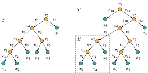
Figure 1: On the left (right) a rooted $X$-tree $T$ ($X^{\prime}$-tree $T^{\prime}$) for $X=\{x_{1},x_{2},\dots,x_{6}\}$ ($X^{\prime}=\{x_{1},x_{2},\dots,x_{8}\}$) with edges $\{e_{1},e_{2},\dots,e_{10}\}$ ($\{e_{1},e_{2},\dots,e_{14}\}$), internal vertices $\{v_{1},v_{2},\dots,v_{5}\}$ ($\{v_{1},v_{2},\dots,v_{7}\}$) and root $v_{5}$ ($v_{7}$). $H$ is a pendant subtree of $T^{\prime}$.

Then, for a rooted phylogenetic $X$-tree $\hat{T}=(T,\ell)$, we call the linear function $\varphi_{\hat{T}}:X\to\mathbb{R}_{\geq 0}^{n}$ defined by

$$\varphi_{\hat{T}}(x)=\sum_{e\in E}\gamma(x,e)\ell(e)$$

a diversity index of $\hat{T}$ where, for $x\in X$, $e\in E$, the $\gamma(x,e)$ are non-negative real numbers such that

(1) $$~{}\sum_{x\in X}\gamma(x,e)=1~{}~{}~{}~{}~{}~{}~{}~{}~{}~{}~{}~{}~{}~{}~{}~{}~{}~{}\,\forall\,e\in E,$$

(2) $$\,~{}~{}~{}~{}~{}~{}~{}\gamma(x,e)=0~{}~{}~{}~{}~{}~{}~{}~{}~{}~{}~{}~{}~{}~{}~{}~{}~{}~{}\,\forall\,x\in X,e\in E\setminus P(x),$$

(3) $$\begin{aligned} \begin{cases}\gamma(x^{1},e_{1})&=\gamma(x^{2},e_{2})~{}~{}~{}~{}~{}~{}~{}~{}~{}\forall\,v_{1},v_{2}\in V,\,x^{i}\in X[v_{i}],\,e_{i}=(u_{i},v_{i})\in E,\\ &~{}~{}~{}~{}~{}~{}~{}~{}~{}~{}~{}~{}~{}~{}~{}~{}~{}~{}~{}~{}~{}~{}~{}~{}~{}~{}~{}~{}~{}~{}T[v_{1}]\cong T[v_{2}],~{}\phi_{1}(x^{1})=\phi_{2}(x^{2}),\\ \gamma(x^{1},e)&=\gamma(x^{2},e)~{}~{}~{}~{}~{}~{}~{}~{}~{}~{}\,\forall\,e=(u,v)\in E,\,x^{1},x^{2}\in X[v],\,T[v]~{}\text{balanced}.\end{cases}\end{aligned}$$

Diversity indices are mainly used in conservation settings to assist with prioritization of resources. In particular, they inform decisions about which species should be most highly protected. However, different diversity indices can lead to quite distinct priorities and conservation strategies, making the choice of index important. The great expense and long-term nature of conservation projects both reinforce the need to make the best possible decisions.

Over recent years, the properties of various diversity indices have been studied as a first step towards understanding which indices suit which applications [4, 5, 7, 8]. Yet this approach usually involves investigating only well-known indices, that is, those constructed to reflect certain evolutionary and fairness assumptions and not primarily with regard to any useful properties. For example, choosing numbers $\gamma(x,e)$, for $x\in X$, $e\in E$, such that

$$\gamma(x,(u,v)) =\frac{1}{|X[v]|}~{} \forall\,x\in X,\,(u,v)\in E$$

defines the Fair Proportion Index [5]. This index is defined based on the assumption that all species with a common ancestor $v$ should be treated uniformly. We take the opposite approach by imposing properties of diversity indices without additional assumptions. Specifically, we study the combinatorial properties of diversity indices to aid the construction of diversity indices which are optimal with respect to a selection criterion in future research.

Observe that the notion of $H$-balanced subtrees captures local subtree structures $H$ whose replacement by singleton vertices in $T$ yields a balanced subtree $S$ of $T$ with $p$ leaves. For example, on the right in Figure 1, replacing all pendant subtrees isomorphic to $H$ by their root yields the balanced subtree $S$ with edge set $\{e_{8},e_{9}\}$. In effect, constraints (3) ensure that $S$ is treated by any diversity index like a balanced pendant subtree of $T$ even though $S$ is not a pendant subtree. For the image $s$ of $\varphi_{\hat{T}}$, such that $\varphi_{\hat{T}}(x_{i})=s_{i}$ for all $i\in\{1,\dots,n\}$, we call $s_{i}$ the diversity index score of taxon $x_{i}$. Finally, we denote the set of images of diversity indices $\varphi_{\hat{T}}$ by $\mathcal{P}(T,\ell)$ and call it the diversity index polytope.

Our primary motivation to study the diversity index polytope is its usefulness for conservation projects. However, since we take a purely combinatorial approach, extensions of the diversity index polytope are of interest, too. We will see that the diversity index polytope does not have a large number of facets because of the independence conditions (2) on subtree structures. By introducing the notion of a diversity ranking [5], i.e., a partial order on the taxa to determine which species contribute more to the biodiversity of a population (in the face of extinction events), more dependencies between the vertices of $\mathcal{P}(T,\ell)$ arise. Thus, this article provides the necessary ground work to pose questions of interest to the broader operations resesarch community.

In Section 2 we introduce some notation and background information on phylogenetic diversity indices that will prove useful to describe $\mathcal{P}(T,\ell)$. In Section 3, we investigate the combinatorial properties of diversity indices to prove a minimal compact description of $\mathcal{P}(T,\ell)$. In Section 4 we discuss extensions of $\mathcal{P}(T,\ell)$ and further research directions.

2 Notation and background

Let $T$ be a rooted $X$-tree. We write $V_{\text{int}}(T)$, $V(T)$ and $E(T)$ to refer to the set of interior vertices, all vertices and all edges of $T$, respectively. For an edge length function $\ell:E(T)\to\mathbb{R}_{\geq 0}$, to simplify our notation, we denote any restriction of $\ell$ to subsets of $E(T)$ by $\ell$, too. For a diversity index $\varphi_{\hat{T}}$ we refer to conditions (1), (2) and (3) as the convexity condition, descent condition, and neutrality conditions, respectively. The following examples illustrates the restriction to the affine subspace defined by these conditions:

Example 1.

Consider the rooted $X$-tree $T$ on the left in Figure 1, any edge length function $\ell$ on $E(T)$ and any diversity index $\varphi_{(T,\ell)}$. Then, we have $\gamma(x_{i},e_{i})=1$ and $\gamma(x_{j},e_{i})=0$ for all $i,j\in\{1,\dots,6\},i\neq j$ due to the convexity and descent condition. Moreover, $x_{1},x_{2}\in X[v_{1}]$, $x_{4},x_{5}\in X[v_{3}]$ and $T[v_{1}],T[v_{3}]$ are balanced, i.e.,

$$\gamma(x_{1},e_{7})=\gamma(x_{2},e_{7})=\frac{1}{2}~{}~{}~{}\text{and}~{}~{}~{}\gamma(x_{4},e_{9})=\gamma(x_{5},e_{9})=\frac{1}{2}$$

by all three conditions (1), (2) and (3) together.

For $s\in\mathcal{P}(T,\ell)$, we can write $s=\Gamma_{T}l$ for a suitable matrix $\Gamma_{T}\in\mathbb{R}^{n\times|E(T)|}$ of real numbers $\gamma(x,e)$ and a vector $l\in\mathbb{R}^{|E(T)|}$ of edge lengths. Moreover, $\Gamma_{T}(e)$ denotes the column vector of $\Gamma_{T}$ corresponding to edge $e\in E(T)$. For $i\in\{1,\dots,n\}$, we also refer to the diversity index score $s_{i}$ as an allocation of edge lengths to taxon $x_{i}$. Hence, a diversity index can be viewed as an allocation of the total edge weights to the leaves. Our description of $\mathcal{P}(T,\ell)$ will keep in mind the goal of maximizing and minimizing these scores for either individual leaves or for sets of leaves. Then, to localize the allocation of edge lengths, Manson and Steel [8] introduced the notion of consistency for diversity indices: let $\hat{T}=(T,\ell)$ be a rooted phylogenetic $X$-tree and let $\varphi_{\hat{T}}$ be a diversity index of $\hat{T}$. Then, we call $\varphi_{\hat{T}}$ consistent if and only if for all $v\in V_{\text{int}}(T)$, $e_{1},e_{2}\in P(v)$ there exists $k\in\mathbb{R}_{\geq 0}$ such that

(4) $$\sum_{x\in X[w]}\gamma(x,e_{1})=k\cdot\sum_{x\in X[w]}\gamma(x,e_{2})~{} \forall\,(v,w)\in E(T).$$

We call the constants $k$ the consistency constants of $\varphi_{\hat{T}}$ and condition (4) the consistency condition. We illustrate the definition of consistency in the following example:

Example 2.

Consider the rooted $X$-tree $T$ on the left in Figure 1 and any edge length function $\ell$ on $E(T)$. Let $\hat{T}=(T,\ell)$ and let $\varphi_{\hat{T}}$ be a consistent diversity index of $\hat{T}$. Then, continuing Example 1,

$$\Gamma_{T}=\left(\begin{array}[]{cccccccccc}1&0&0&0&0&0&\frac{1}{2}&\gamma(x_{1},e_{8})&0&\gamma(x_{1},e_{10})\\ 0&1&0&0&0&0&\frac{1}{2}&\gamma(x_{2},e_{8})&0&\gamma(x_{2},e_{10})\\ 0&0&1&0&0&0&0&\gamma(x_{3},e_{8})&0&\gamma(x_{3},e_{10})\\ 0&0&0&1&0&0&0&0&\frac{1}{2}&\gamma(x_{4},e_{10})\\ 0&0&0&0&1&0&0&0&\frac{1}{2}&\gamma(x_{5},e_{10})\\ 0&0&0&0&0&1&0&0&0&0\end{array}\right)$$

is the matrix of numbers $\gamma(x,e)$ defining $\varphi_{\hat{T}}$. Observe that $\varphi_{\hat{T}}$ is not consistent if we choose $\Gamma_{T}(e_{8})=(1/3,1/3,1/3,0,0,0)$ and $\Gamma_{T}(e_{10})=(1/8,1/8,1/2,1/8,1/8,0)$ because

$$\gamma(x_{1},e_{8})+\gamma(x_{2},e_{8})=\frac{2}{3}=\frac{8}{3}\cdot\frac{1}{4}=\frac{8}{3}\cdot\left(\gamma(x_{1},e_{10})+\gamma(x_{2},e_{10})\right),$$

but

$$\gamma(x_{3},e_{8})=\frac{1}{3}=\frac{2}{3}\cdot\frac{1}{2}=\frac{2}{3}\cdot\gamma(x_{3},e_{10}).$$

If instead we choose $\Gamma_{T}(e_{10})=(1/7,1/7,1/7,2/7,2/7,0)$, then

$$\gamma(x_{1},e_{8})+\gamma(x_{2},e_{8}) =\frac{2}{3}=\frac{7}{3}\cdot\frac{2}{7}=\frac{7}{3}\cdot\left(\gamma(x_{1},e_{10})+\gamma(x_{2},e_{10})\right),$$

$$\gamma(x_{3},e_{8}) =\frac{1}{3}=\frac{7}{3}\cdot\frac{1}{7}=\frac{7}{3}\cdot\gamma(x_{3},e_{10}),$$

i.e., we find consistency constant $k=7/3$ for vertex $v_{2}$ and edges $e_{8},e_{10}$. Furthermore,

$$\gamma(x_{i},e_{7}) =\frac{1}{2}=\frac{3}{2}\cdot\frac{1}{3}=\frac{3}{2}\cdot\gamma(x_{i},e_{8})~{} \forall\,i\in\{1,2\},$$

$$\gamma(x_{i},e_{7}) =\frac{1}{2}=\frac{7}{2}\cdot\frac{1}{7}=\frac{7}{2}\cdot\gamma(x_{i},e_{10})~{} \forall\,i\in\{1,2\},$$

$$\gamma(x_{i},e_{9}) =\frac{1}{2}=\frac{7}{4}\cdot\frac{2}{7}=\frac{7}{4}\cdot\gamma(x_{i},e_{10})~{} \forall\,i\in\{4,5\},$$

which means $k=3/2$ for $v_{1},e_{7},e_{8}$, $k=7/2$ for $v_{1},e_{7},e_{10}$ and $k=7/4$ for $v_{3},e_{9},e_{10}$. Hence, $\varphi_{\hat{T}}$ is consistent for the second choice of $\Gamma_{T}(e_{10})$. Observe that imposing the consistency condition equations reduces the number of free choices for entries of $\Gamma_{T}$ by 4. This means, together with the convexity condition, we reduce the remaining $8$ free choices of numbers $\gamma(x,e)$ to define $\Gamma_{T}$ to $2$.

We call the number of free choices we can make to define a consistent diversity index of a rooted phylogenetic $X$-tree $\hat{T}=(T,\ell)$ the degrees of freedom $d_{\hat{T}}$ of $\hat{T}$. In Example 2 we observed that $d_{\hat{T}}=2$. To generalize this observation we characterize matrices $\Gamma_{T}$ as follows:

Proposition 2.1.

Let $\hat{T}=(T,\ell)$ be a rooted phylogenetic $X$-tree and let $\varphi_{\hat{T}}$ be a consistent diversity index. For $e=(u,v)\in E(T)$, if $T[v]$ is $H$-balanced for some pendant subtree $H$ of $T[v]$ (not $H$-balanced for any graph $H$), then the consistency condition implies that there exists no (exactly one) free choice of entries in $\Gamma_{T}(e)$ independent of $\Gamma_{T}(e^{\prime})$ for all edges $e^{\prime}$ in $T[v]$.

Proof 2.2.

Let $e=(u,v)\in E(T)$. First, assume $T[v]$ is balanced. Then the neutrality conditions imply that $\gamma(x,e)$ has the same value for all $x\in X[v]$. Hence, we conclude by the convexity and descent condition that there is no free choice for any entry of $\Gamma_{T}$ and

$$\gamma(x,e)=\begin{cases}\frac{1}{|X[v]|}&\text{if $x\in X[v]$},\\ 0&\text{otherwise.}\end{cases}$$

Next, assume that $T[v]$ is not balanced, but $T[v]$ is $H$-balanced for some non-singleton subtree $H$ of $T[v]$. Let $\left\{T\left[v_{i(1)}\right],\dots,T\left[v_{i(p)}\right]\right\}$ be the collection of pendant subtrees of $T[v]$ isomorphic to $H$. For $i(k)$, $k\in\{1,\dots,p\}$, suppose, with a view to contradiction, that $T^{\prime}=T\left[v_{i(k)}\right]$ is $G$-balanced for some pendant subtree $G$ of $T^{\prime}$. Then, $T[v]$ is $G$-balanced, too. This contradicts the fact that $T[v]$ is $T^{\prime}$-balanced. Therefore, $T^{\prime}$ is not $G$-balanced for all pendant subtrees $G$ of $T^{\prime}$. Let $e^{\prime}=(u^{\prime},v^{\prime})\in E(T)$ such that $T^{\prime}=T[v^{\prime}]$. Then, by induction on $n$, considering our claim for $T^{\prime}$ instead of $T$ we deduce that there exists exactly one free choice of entries in $\Gamma_{T}(e^{\prime})$ independent of $\Gamma_{T}(e^{\prime\prime})$ for all edges $e^{\prime\prime}$ in $T[v^{\prime}]$. This means there exists no free choice of entries in $\Gamma_{T}(e)$ independent of $\Gamma_{T}(e^{\prime})$. Thus, our claim follows.

Finally, assume $T[v]$ is not $H$-balanced for any graph $H$. Consider $e_{1}=(v,w_{1})$, $e_{2}=(v,w_{2})\in E(T)$. There exist consistency constants $k_{1}$ and $k_{2}$ for $w_{1},e_{1},e$ and $w_{2},e_{2},e$, respectively. The same argument can be extended to all edges in $T[w_{1}]$ and $T[w_{2}]$. Thus, there exists exactly one free choice of entries in $\Gamma_{T}(e)$ independent of $\Gamma_{T}(e^{\prime})$ for all $e^{\prime}$ in $T[w_{1}]$. The same conclusion can be drawn for $T[w_{2}]$. Hence, by the convexity condition there exists exactly one free choice of entries in $\Gamma_{T}(e)$ independent of $\Gamma_{T}(e^{\prime})$ for all $e^{\prime}$ in $T[v]$.

Example 1.

Continuing Example 2, we know from Proposition 2.1 that $\Gamma_{T}$ is uniquely defined by exactly one free choice of entries both in $\Gamma_{T}(e_{8})$ and $\Gamma_{T}(e_{10})$ independent of $\Gamma_{T}(e^{\prime})$ for all edges $e^{\prime}$ in $T[v_{2}]$ and $T[v_{4}]$, respectively. If instead we consider $T^{\prime}$ on the right in Figure 1, then applying Proposition 2.1 yields exactly three free choices: one for entries in $\Gamma_{T}(e_{8})$, $\Gamma_{T}(e_{9})$ and $\Gamma_{T}(e_{14})$, respectively. However, $d_{(T^{\prime},\ell)}=2$ because $T[v_{2}]\cong T[v_{3}]$.

Example 1 illustrates that consistency conditions do not localize all neutrality conditions to their respective edges. Specifically, edges which satisfy a neutrality condition but do not induce intersecting pendant subtrees cannot be localized to a single vertex. Therefore, we consider the equivalence relation on $E(T)$ induced by the neutrality conditions which invoke the isomorphisms $T[v_{1}]\cong T[v_{2}]$ in (3). Let $E_{1}(T),\dots,E_{p}(T)\subset E(T)$ be the resulting equivalence classes. For $E_{i}=\{(u,v)\}$, $i\in\{1,\dots,p\}$, and $T[v]$ not $H$-balanced for any graph $H$, we call $(u,v)$ a free edge. In other words, we can make exactly one free choice to define the allocation of the length of a free edge to taxa without violating any neutrality or consistency condition (see Proposition 2.1). However, if we deal with an edge for which Proposition 2.1 offers one free choice but which is not a free edge, we have to make sure that we make this one free choice exactly once when defining $\Gamma_{T}$.

To this end, let $E_{f}\subset E(T)$ ($E_{c}\subset E(T)$) denote a set of representatives $(u,v)$ of the equivalence classes $E_{1}(T),\dots,E_{p}(T)$ such that $T[v]$ is not $H$-balanced for any graph $H$ ($T[v]$ is $H$-balanced for some graph $H$). We call $E_{f}$ a set of independent edges because when specifying the submatrix $\Gamma_{T}^{\prime}$ of $\Gamma_{T}$ constituted by columns $\Gamma_{T}(e)$, $e\in E_{f}$, we can treat every edge in $\Gamma_{T}^{\prime}$ like we treat a free edge in $\Gamma_{T}$. In other words, $\Gamma_{T}$ is uniquely defined by exactly one free choice for each edge $e\in E_{f}$. We call $E_{c}$ a set of dependent edges because we know from Proposition 2.1 that there exists no free choice of entries in $\Gamma_{T}(e)$ independent of all other columns in $\Gamma_{T}$ under consistency conditions. We denote the set of subsets $E_{f}$ by $\mathcal{F}(T)$ and $U_{f}(T)$ as the union of all sets in $\mathcal{F}(T)$. Similarly, we denote the set of subsets $E_{c}$ by $\mathcal{C}(T)$ and $U_{c}(T)$ as the union of all sets in $\mathcal{C}(T)$. Notice that for all $E_{f}\in\mathcal{F}(T)$ there exists $E_{c}\in\mathcal{C}(T)$ such that, for $e=(u,v)\in E_{c}$, either $T[v]$ is balanced or $\Gamma_{T}(e)$ is uniquely defined by $\Gamma_{T}(e^{\prime})$ for some $e^{\prime}\in E(T[v])\cap E_{f}$ because only edges in $U_{f}(T)$ offer free choices to define $\Gamma_{T}$ under consistency conditions. The same holds for subsets of $E_{f}$ and suitable subsets of $E_{c}$. In this case we call (subsets of) $E_{c}$ dependent on (subsets of) $E_{f}$. Throughout this article we will use sets $E_{f}\in\mathcal{F}(T)$ to define matrices $\Gamma_{T}$ and only consider sets $E_{c}\in\mathcal{C}(T)$ dependent on $E_{f}$ when calculating an allocation of edge lengths to taxa. Moreover, we close the gap in characterizing degrees of freedom, as illustrated in Example 1, by observing that

$$d_{\hat{T}}=|E_{f}|~{}~{}~{}~{}~{}\forall\,E_{f}\in\mathcal{F}(T).$$

Another aspect of describing the symmetry conditions of consistent diversity indices concerns not only localizing them to edges but taxa, too. This is of particular interest when we will calculate diversity index scores. To this end, let $\hat{X}_{\hat{x},e}\subseteq X$, $\hat{x}\in\hat{X}_{\hat{x},e}$, $e\in E(T)$, denote the set of maximum cardinality of taxa with constant $\gamma(\hat{x},e)$ induced by neutrality and consistency conditions.

Example 2.

Consider the rooted $X$-tree on the left in Figure 1. We have $\hat{X}_{x_{1},e}=\{x_{1},x_{2}\}$ for all edges $e\in\{e_{7},e_{8},e_{10}\}$ because (i) taxa $x_{1}$ and $x_{2}$ satisfy a neutrality condition with respect to edge $e_{7}$; (ii) edges $e_{8}$ and $e_{10}$ satisfy consistency conditions for $v_{1},e_{7},e_{8}$ and $v_{1},e_{7},e_{10}$, respectively. In this example the dependency of $\hat{X}_{x_{1},e}$ on edges $e\in P(x_{1})$ is redundant. However, in general this is not the case. For example, on the right in Figure 1, we have $\hat{X}_{x_{1},e_{7}}=\hat{X}_{x_{1},e_{8}}=\{x_{1},x_{2}\}$ and $\hat{X}_{x_{1},e_{10}}=\hat{X}_{x_{1},e_{14}}=\{x_{1},x_{2},x_{4},x_{7}\}$ because $e_{10}$ satisfies neutrality conditions

$$\gamma(x_{1},e_{10})=\gamma(x_{4},e_{10}),~{}\gamma(x_{2},e_{10})=\gamma(x_{7},e_{10})$$

or

$$\gamma(x_{1},e_{10})=\gamma(x_{7},e_{10}),~{}\gamma(x_{2},e_{10})=\gamma(x_{4},e_{10})$$

and consistency conditions for $v_{2},e_{8},e_{10}$ and $v_{2},e_{9},e_{10}$, i.e.,

$$\gamma(x_{1},e_{10})=\gamma(x_{2},e_{10}),~{}\gamma(x_{4},e_{10})=\gamma(x_{7},e_{10}).$$

For $Y\subseteq X$, let $T(Y)$ denote the induced subtree of $T$ on leafset $Y$ and for $x_{i}\in Y$ and $Z\subseteq Y$, let $F(Y-x_{i})$ and $F(Y-Z)$ denote the forest we obtain from $T(Y)$ by removing the edges in path(s) $P(x_{i})$ and $P(z_{i})$, $z_{i}\in Z$, and deleting resulting singletons, respectively. For $x_{j}\in Y$, $x_{j}\neq x_{i}$, let $T_{j}(Y-x_{i})$ denote the connected component of $F(Y-x_{i})$ which has $x_{j}$ among its leaves. Clearly, $T_{j}(Y-x_{i})$ forms an equivalence class in $Y\setminus\{x_{i}\}$. Furthermore, for $E_{f}\in\mathcal{F}(T)$, let $E_{f|i}\subseteq E_{f}$ denote the constriction of $E_{f}$ to edges in $F(X-x_{i})$. Moreover, let $\mathcal{I}(x_{i},Y,E_{f})\subseteq Y$ be a set of maximum cardinality such that

1. $T_{j}(Y-x_{i})\neq T_{k}(Y-x_{i})$ for all $x_{j},x_{k}\in\mathcal{I}(x_{i},Y,E_{f})$,

2. the maximum number of neutrality and consistency conditions holds between pairs of taxa in $\{(x_{i},x_{j})\,:\,x_{j}\in\mathcal{I}(x_{i},Y,E_{f})\}$ among all valid choices for $\mathcal{I}(x_{i},Y,E_{f})$,

Observe that $\mathcal{I}(x_{i},Y,E_{f})$ is not uniquely defined:

Example 3.

For the rooted $X^{\prime}$-tree on the right in Figure 1, $E_{f}=\{e_{8},e_{14}\}$ is a set of independent edges and we can choose $\mathcal{I}(x_{1},X,E_{f})=\{x_{2},x_{3},x_{j},x_{6},x_{8}\}$ for $j\in\{4,7\}$ to satisfy both properties 1 and 2.

The set $\mathcal{I}(x_{i},Y,E_{f})$ can be viewed as a specific set of representatives of the equivalence classes $T_{j}(Y-x_{i})$. We will use this set in the next section to study the allocation of edges in $E_{f|i}$ to taxa in $Y\setminus\{x_{i}\}$ without violating neutrality and consistency conditions. Indeed, if we want to maximize the allocation of edge lengths to taxa in $Y$ under all conditions for diversity indices, starting with an allocation of edge lengths to taxon $x_{i}$, then property 2 excludes choices of representatives which obstruct maximality. As another prerequisite for this analysis, we provide useful formulas for diversity index scores of a single taxon. First, for $Y\subseteq X$, $\hat{x}\in Y$ and a pendant subtree $S$ of $T(Y)$, we call

$$\text{LB}(\hat{x},T) =\sum_{\begin{subarray}{c}e=(u,v)\in P(\hat{x})\cap U_{c}(T)\\ T[v]\text{ balanced}\end{subarray}}\frac{\ell(e)}{\left|\hat{X}_{\hat{x},e}\right|}$$

and

$$\text{UB}\left(\hat{x},S\right) =\,\text{LB}(\hat{x},T)+\sum_{\begin{subarray}{c}e=(u,v)\in P(\hat{x})\cap U_{c}(S)\\ T[v]\text{ not balanced}\end{subarray}}\frac{\ell(e)}{\left|\hat{X}_{\hat{x},e}\right|}+\sum_{e\in P(\hat{x})\cap U_{f}(S)}\frac{\ell(e)}{\left|\hat{X}_{\hat{x},e}\right|}$$

the minimum allocation from $T$ and maximum allocation from $S$ to $\hat{x}$, respectively. As shorthand notations, let $\hat{X}_{\hat{x}}$ denote the set defining the largest denominator in the definition of LB$(x_{i},T)$ and let $N(\hat{x})=\left|\hat{X}_{\hat{x}}\right|$. Secondly, let $Z\subseteq Y$, $E_{f}\in\mathcal{F}(T)$ and let $E^{-}$ be a subset of a set in $\mathcal{F}(S)$ with $E^{-}\subseteq E_{f}$. Let $\mathcal{E}\left(\hat{x},E^{-},E_{f},Z\right)$ denote the union of $P(\hat{x})\cap E^{-}$ and the set of edges $e\in P(\hat{x})\cap E(S)$ satisfying the following condition:

$$\exists\,z\in Z,\,i\in\{1,\dots,p\}\text{ such that }e\in E_{i}(T),\,P(z)\cap E_{f}\cap E_{i}(T)\neq\emptyset,$$

$$~{}~{}~{}~{}~{}~{}~{}~{}~{}~{}~{}\text{$\hat{x}$ and $z$ satisfy a neutrality condition with respect to $e$}.$$

Set $\mathcal{E}\left(\hat{x},E^{-},E_{f},Z\right)$ encodes the edges in $P(\hat{x})\cap E(S)$ which either appear in $E^{-}$ or in the same equivalence class as an edge in $P(z)\cap E_{f}$, $z\in Z$. Hence, if $Z=X$, then $\mathcal{E}(\hat{x},E^{-},E_{f},Z)=E_{f}^{\prime}\in\mathcal{F}(S)$ with $|P(\hat{x})\cap E_{f}^{\prime}|$ maximum. Let $\mathcal{E}^{*}\left(\hat{x},E^{-},E_{f},Z\right)$ denote the extension of $\mathcal{E}\left(\hat{x},E^{-},E_{f},Z\right)$ by sets $E_{c}^{\prime}$ with

$$E_{c}^{\prime}\subseteq E_{c}\in\mathcal{C}(S),\,\left|P(\hat{x})\cap E_{c}^{\prime}\right|\text{\,maximal},\,E_{c}^{\prime}\text{ dependent on }\mathcal{E}(\hat{x},E^{-},E_{f},Z).$$

Hence, if $Z=X$, then $\mathcal{E}^{*}(\hat{x},E^{-},E_{f},Z)=P(\hat{x})\cap E(S)$. Now, we call

(5) $$\text{MB}\left(\hat{x},E^{-},E_{f},Z,S\right)=\sum_{e\in\mathcal{E}^{*}\left(\hat{x},E^{-},E_{f},Z\right)}\frac{\ell(e)}{\left|\hat{X}_{\hat{x},e}\right|}$$

the intermediate allocation from $S$ to $\hat{x}$ with respect to $E^{-},E_{f}$ and $Z$. By definition we know that

$$\text{MB}\left(\hat{x},\emptyset,E_{f},\emptyset,T\right)=\,\text{LB}(\hat{x},T)~{}~{}~{}~{}\text{and}~{}~{}~{}~{}\text{MB}\left(\hat{x},\emptyset,E_{f},X,T\right)=\,\text{UB}(\hat{x},T).$$

Otherwise, for suitable choices of $E^{-}$ and $S$, we can view (5) as a partial maximum allocation:

Lemma 2.3.

Let $\hat{T}=(T,\ell)$ be a rooted phylogenetic $X$-tree, $Y\subseteq X$, $\hat{x}\in Y$, $E_{f}\in\mathcal{F}(T)$, a pendant subtree $S$ of $T(Y)$ rooted in $v$ with $\hat{x}\in X[v]$ and let $E^{-}$ denote the constriction of $E_{f}$ to edges in  $S$. Let $\varphi_{(T(Y),\ell)}$ be a consistent diversity index with $\gamma(\hat{x},e)$ maximum for all $e\in P(\hat{x})\cap E(S)$. Then,

$$\varphi_{(T(Y),\ell)}(\hat{x})=\,\text{MB}\left(\hat{x},E^{-},E_{f},Y\setminus X[v],S\right).$$

Proof 2.4.

Let $E_{f}^{\prime}\in\mathcal{F}(T(Y))$ with $|P(\hat{x})\cap E_{f}^{\prime}|$ maximum and let $E^{--}$ denote the constriction of $E_{f}^{\prime}$ to edges in $S$. This means, by definition

$$P(\hat{x})\cap E^{--}=\mathcal{E}(\hat{x},E^{-},E_{f},Y\setminus X[v]).$$

Let $E_{c}\in\mathcal{C}(S)$, $|P(\hat{x})\cap E_{c}|$ maximal, be dependent on $E^{--}$. Then, by the choice of $\varphi_{(T(Y),\ell)}$, we have

$$\varphi_{(T(Y),\ell)}(\hat{x}) =\sum_{e\in P(\hat{x})\cap E(T(Y))}\gamma(\hat{x},e)\ell(e)=\sum_{e\in P(\hat{x})\cap\left(E^{--}\cup E_{c}\right)}\gamma(\hat{x},e)\ell(e)$$

$$=\sum_{e\in\mathcal{E}^{*}\left(\hat{x},E^{-},E_{f},Y\setminus X[v]\right)}\gamma(\hat{x},e)\ell(e)=\,\text{MB}\left(\hat{x},E^{-},E_{f},Y\setminus X[v],S\right).$$

To conclude this section, we summarize some additional properties of diversity indices investigated by Manson and Steel [8] as follows:

Proposition 2.5.

Let $\hat{T}=(T,\ell)$ be a rooted phylogenetic $X$-tree.

1. For every diversity index $\varphi_{\hat{T}}$ which is not consistent there exists a consistent diversity index with the same diversity index scores as $\varphi_{\hat{T}}$.

2. For any diversity index $\varphi_{\hat{T}}$ and $x\in X$, we have $\varphi_{\hat{T}}(x)\in[\text{LB}(x,T),\text{UB}(x,T)]$.

3. $\mathcal{P}(T,\ell)$ is a finite convex set.

4. If all diversity indices are consistent, then the dimension of $\mathcal{P}(T,\ell)$ is the maximum number of free choices which specify $\Gamma_{T}$ for any $\Gamma_{T}l\in\mathcal{P}(T,\ell)$.

3 On the combinatorial properties of diversity indices

In this section we give a compact description of the diversity index polytope $\mathcal{P}(T,\ell)$ by providing all facet-defining inequalities of an embedding in an appropriate vector space. To this end, we assume that all diversity indices are consistent. In general this assumption does not hold. However, as we will see, consistent diversity indices are sufficient to describe all facets of $\mathcal{P}(T,\ell)$. First, we use Proposition 2.5.2 to characterize the set of extreme points of $\mathcal{P}(T,\ell)$. The proof is straightforward using the properties of $\mathcal{P}(T,\ell)$ (see Appendix A).

Proposition 3.1.

Let $\hat{T}=(T,\ell)$ be a rooted phylogenetic $X$-tree and let $E_{f}\in\mathcal{F}(T)$. Then, the set of extreme points of $\mathcal{P}(T,\ell)$ is given by

$$\mathrm{ext}(T,\ell)= \left\{\Gamma_{T}l\,:\,\text{choose a maximum or minimum value}\right.$$

$$~{}~{}~{}~{}~{}~{}~{}~{}~{}\left.\text{for every free choice in }\Gamma_{T}(e),\,e\in E_{f}\right\}.$$

Next, consider the dimension of $\mathcal{P}(T,\ell)$ which we denote by dim$(T,\ell)$. From Proposition 2.5.4 we know that dim$(T,\ell)=d_{\hat{T}}$. This insight enables us to give another characterization of $\mathcal{P}(T,\ell)$ different from Proposition 3.1. To this end, we first define a recursive formula to calculate the allocation of edge lengths to different pendant subtrees and then use this formula to characterize $\mathcal{P}(T,\ell)$ as an intersection of a finite number of halfspaces.

3.1 A description of the diversity index polytope by linear inequalities

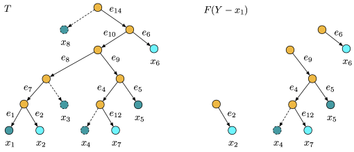
Figure 2: On the left a rooted $X$-tree $T$ for $X=\{x_{1},x_{2},\dots,x_{8}\}$. For $Y=\{x_{1},x_{2},x_{5},x_{6},x_{7}\}$, the induced subtree $T(Y)$ of $T$ is shown in non-dashed lines. The set $\mathcal{I}(x_{1},Y,\{e_{8},e_{14}\})=\{x_{2},x_{6},x_{7}\}$ is shown in light blue. On the right we have the resulting forest $F(Y-x_{1})$.

For $Y\subseteq X$, recall from the previous section that both the minimum allocation from $T$ to $\hat{x}$ and the maximum allocation from $S$ to $\hat{x}$ can be calculated independently for all $\hat{x}\in Y$. However, for $s\in\mathcal{P}(T,\ell)$, whenever we want to bound linear functions in $s$ we have to analyse diversity index scores in the interval $(\,\text{LB}(\hat{x},T),\,\text{UB}(\hat{x},S))$. We have shown in Lemma 2.3 that some of the arising dependencies for the allocation of edge lengths to taxa $Y$ can be encoded by the intermediate allocation (5). We expand on this approach by combining multiple intermediate allocations to bound linear functions in $s$. To this end, for $x_{i}\in Y$ and $e\in E(T)$, let

$$N(x_{i},e,Y)=\left|\hat{X}_{x_{i},e}\cap\bigcup_{y\in Y}\hat{X}_{y}\right|/\left|\hat{X}_{x_{i},e}\right|\in[0,1].$$

We call

$$\text{LB}\left(x_{i},Y,T\right)=\sum_{\begin{subarray}{c}e=(u,v)\in P(x_{i})\cap U_{c}(T)\\ T[v]\text{ balanced}\end{subarray}}N(x_{i},e,Y)\cdot\ell(e)=\sum_{\begin{subarray}{c}e=(u,v)\in P(x_{i})\cap U_{c}(T)\\ T[v]\text{ balanced}\end{subarray}}\ell(e)$$

the minimum allocation for $T(Y)$ with respect to $x_{i}$. Here, we have $N(x_{i},e,Y)=1$ because $T[v]$ is balanced, i.e., $\hat{X}_{x_{i},(u,v)}\subseteq\hat{X}_{x_{i}}$. Also recall that $\,\text{LB}(x_{i},T)$ is a weighted version of the summation $\text{LB}\left(x_{i},Y,T\right)$. Then, for $Z\subseteq Y$, $E_{f}\in\mathcal{F}(T)$, the constriction $E^{-}$ of $E_{f}$ to edges in $T(Z)$, we extend the intermediate allocation from $T(Z)$ to $x_{i}$ to

(6) $$r_{i}(T(Z),E^{-})$$

$$=\sum_{e\in\mathcal{E}^{*}(x_{i},E^{-},E_{f},Y\setminus Z)}N(x_{i},e,Y)\cdot\ell(e)+\sum_{x_{j}\in\mathcal{I}\left(x_{i},Z,E^{-}\right)}r_{j}\left(T_{j}(Z-x_{i}),E_{f|i}\right)$$

and call it the maximum allocation for $T(Z)$ with respect to $x_{i}$, $E^{-}$ and $E_{f}$. With recursion (6) at hand we define

(7) $$r\left(T(Z),E_{f}\right)=\max_{x_{i}\in Z}~{}r_{i}\left(T(Z),E_{f}\right)-\sum_{x_{i}\in Z}\text{LB}\left(x_{i},Y,T\right),$$

and call it the maximum allocation for $T(Z)$ with respect to $E_{f}$.

Example 4.

Consider the rooted $X$-tree $T$ on the left in Figure 2 and the corresponding sets $Y=\{x_{1},x_{2},x_{5},x_{6},x_{7}\}$ and $\mathcal{I}(x_{1},Y,E_{f})=\{x_{2},x_{6},x_{7}\}$ for the set $E_{f}=\{e_{8},e_{14}\}$ of independent edges. Then, since $E_{c}=\{e_{1},e_{7},e_{10}\}$ is dependent on $E_{f}$ with $|P(x_{1})\cap E_{c}|$ maximum in $\mathcal{C}(T)$, we obtain

$$r_{1}\left(T(Y),E_{f}\right)$$

$$=\sum_{e\in\mathcal{E}^{*}(x_{1},E_{f},E_{f},\emptyset)}N(x_{1},e,Y)\cdot\ell(e)+\sum_{x_{j}\in\mathcal{I}\left(x_{1},Y,E_{f}\right)}r_{j}\left(T_{j}(Y-x_{1}),E_{f|1}\right)$$

$$=\,\text{LB}(x_{1},Y,T)+\sum_{e\in\{e_{8},e_{10},e_{14}\}}\ell(e)+\sum_{x_{j}\in\{x_{2},x_{6},x_{7}\}}r_{j}\left(T_{j}(Y-x_{1}),E_{f|1}\right).$$

Since the constriction $E_{f|1}$ of $E_{f}$ to edges in $F(Y-x_{1})$ is the empty set (see Figure 2),

$$r_{2}\left(T_{2}(Y-x_{1}),E_{f|1}\right)=\sum_{e\in\mathcal{E}^{*}(x_{2},\emptyset,E_{f},Y\setminus\{x_{2}\})}N(x_{i},e,Y)\cdot\ell(e)=\,\text{LB}(x_{2},Y,T).$$

Analogously, $r_{6}\left(T_{6}(Y-x_{1}),E_{f|1}\right)=\,\text{LB}(x_{6},Y,T)$. Similarly, since

$$\mathcal{E}(x_{7},\emptyset,E_{f},\{x_{1},x_{2},x_{6}\})=\{e_{9}\},$$

we get $\mathcal{E}^{*}(x_{7},\emptyset,E_{f},\{x_{1},x_{2},x_{6}\})=\{e_{4},e_{9},e_{12}\}$. Hence, for $T^{\prime}=T_{7}(Y-x_{1})$ we get

$$r_{7}\left(T^{\prime},E_{f|1}\right) =\,\text{LB}(x_{7},Y,T)+\ell(e_{9})+r_{5}\left(T^{\prime}_{5}(\{x_{7}\}-x_{7}),\emptyset\right)$$

$$=\,\text{LB}(x_{7},Y,T)+\ell(e_{9})+\,\text{LB}(x_{5},Y,T).$$

Thus, in total

$$r_{1}\left(T(Y),E_{f}\right)-\sum_{x_{i}\in Y}\text{LB}\left(x_{i},Y,T\right)=\ell(e_{8})+\ell(e_{9})+\ell(e_{10})+\ell(e_{14}).$$

Similarly, if we keep $Y=\{x_{1},x_{2},x_{5},x_{6},x_{7}\}$ but consider taxon $x_{5}$ instead of $x_{1}$, then

$$r_{5}\left(T(Y),E_{f}\right)-\sum_{x_{i}\in Y}\text{LB}(x_{i},Y,T)=\ell(e_{9})+\frac{1}{2}\ell(e_{10})+\frac{1}{2}\ell(e_{14}).$$

If we choose $Y=\{x_{1},x_{5},x_{6}\}$ instead, then $\mathcal{I}(x_{1},Y,E_{f})=\{x_{5},x_{6}\}$. Hence, we obtain $\mathcal{E}(x_{5},\emptyset,E_{f},\{x_{1},x_{6}\})=\emptyset$ and therefore

$$r_{1}\left(T(Y),E_{f}\right)-\sum_{x_{i}\in Y}\text{LB}\left(x_{i},Y,T\right)=\ell(e_{8})+\frac{1}{2}\ell(e_{10})+\frac{1}{2}\ell(e_{14}).$$

Example 4 illustrates that its not clear a-priori which taxa maximize (7) and subsequent recursion steps because of the dependency of numbers $N(x_{i},e,Y)$ on $x_{i}$ and $Y$. However, $x_{i}$ is a maximizer of (7) for a specific choice of $Z$:

Proposition 3.2.

Let $\hat{T}=(T,\ell)$ be a rooted phylogenetic $X$-tree with $d_{\hat{T}}\geq 1$, let $x_{i}\in X$. Then, there exist $E_{f}\in\mathcal{F}(T)$ and $Y\subseteq X$ with $|Y|=d_{\hat{T}}$ such that

(8) $$r\left(T(Y\cup\{x_{i}\}),E_{f}\right)=r_{i}\left(T(Y\cup\{x_{i}\}),E_{f}\right)-\sum_{x_{j}\in Y\cup\{x_{i}\}}\text{LB}(x_{j},Y\cup\{x_{i}\},T).$$

Furthermore, there exists a bijective map $\phi:E_{f}\to Y$ with $e\in P(\phi(e))$ such that $\gamma(\phi(e),e)=0$, $e\in E_{f}$, for the diversity index associated with the allocation on the righthand side of (8). Moreover, $z\notin\hat{X}_{y,e}$ for all $y,z\in Y$, $e\in E(T)$.

Proof 3.3.

Let $E_{f}\in\mathcal{F}(T)$ and let $\varphi_{\hat{T}}^{0}$ be the diversity index defined by coefficients $N\left(x_{i},(u,v),X\right)$, $T[v]$ not balanced, in the calculation of

(9) $$\max~{}r_{i}\left(T,E_{f}\right)-\sum_{x_{k}\in X}\text{LB}(x_{k},X,T).$$

Here, $x_{i}\in X$ is fixed and we maximize all subsequent recursion steps of $r_{i}\left(T,E_{f}\right)$. Let $s^{0}\in\mathcal{P}(T,\ell)$ be the image of $\varphi_{\hat{T}}^{0}$ and let $T_{1}^{\prime},\dots,T_{d}^{\prime}$ be the non-singleton connected components of $T$ which we obtain from the recursion (6) when it terminates in the calculation of (9). Let $E_{f}=E_{0}\cup E_{+}$ be a bipartition of edges $e=(u,v)\in E_{f}$ with $e_{1}=(v,w_{1}),e_{2}=(v,w_{2})\in E(T)$ into edges

1. $e\in E_{0}$ such that $e_{1}\in E\left(T_{p}^{\prime}\right)$ for some $p\in\{1,\dots,d\}$,

2. $e\in E_{+}$ such that $e_{i}\notin E\left(T_{p}^{\prime}\right)$ for all $i\in\{1,2\}$, $p\in\{1,\dots,d\}$.

Then, define

(10) $$x^{e} =\,\text{arg}\,\min\limits_{x_{j}\in X[w_{1}]}\left\{s_{j}^{0}-\,\text{LB}(x_{j},T)\right\}~{} \forall\,e=(u,v)\in E_{0},(v,w_{1})\in E(T).$$

By definition of $E_{0}$, taxa $x^{e}$ are pairwise distinct and $\gamma(x^{e},e)=0$, $e\in E_{0}$, for diversity index $\varphi_{\hat{T}}^{0}$. Next, let $e=(u,v)\in E_{+}$. Recall that in the calculation of (9) edges $e_{1}$ and $e_{2}$ are removed for different reasons. One edge, say $e_{2}$, is removed to be consistent with a maximum allocation of edge $e$ to some taxon $x_{k}$. The other edge $e_{1}$ is removed for a maximum allocation of $e_{1}$ to some taxon $x_{j}\neq x_{k}$. For the latter, let $P$ denote the directed path starting in $v$ and ending in $x_{j}$. Suppose by contradiction $\gamma(x_{j},e)>0$. Since $\ell(e)$ is (partially) allocated to a taxon $x_{k}\in X[w_{2}]$ by $\varphi_{\hat{T}}^{0}$, we know that $x_{j}\in\hat{X}_{x_{k},e}$. This means, there exists an edge $e^{\prime}=(u^{\prime},v^{\prime})\in P(x_{j})\cap P(x_{k})$ such that $T[v^{\prime}]$ is $H$-balanced for some graph $H$ and $v^{\prime},e^{\prime},e$ satisfy a consistency condition. Here, $e=e^{\prime}$ is not possible because $e\in E_{f}$. However, there exists no edge $e^{\prime}\in P(x_{j})\cap P(x_{k})$ with $|P(e^{\prime})|>|P(e)|$ by our choice of $x_{j}$ and $x_{k}$, leading to a contradiction. Thus, $\gamma(x_{j},e)=0$. Let $x^{e}=x_{j}$. Observe that taxa $x^{e}$, $e\in E_{+}$, are pairwise distinct because $x_{j}$ is a singleton component after the removal of the edges in $P$. Hence, for $Y=\{x^{e}\,:\,e\in E_{f}\}$, we obtain a bijective map $\phi:E_{f}\to Y$ with $e\in P(\phi(e))$ and $\gamma(\phi(e),e)=0$ in $\varphi_{\hat{T}}^{0}$ for all $e\in E_{f}$. Since $z\notin\hat{X}_{y,e}$ for all $y,z\in Y$, $e\in E(T)$, by our construction of $Y$, diversity index scores of pairs of taxa $x_{k},x_{l}\in Y$ can be dependent only if a neutrality condition $\gamma(x_{k},e_{k})=\gamma(x_{l},e_{l})$ holds with either $e_{k}\in E_{f}$ or $e_{l}\in E_{f}$. Recall that taxa in $Y$ have maximum diversity index scores in $s^{0}$ within the connected components they are representatives of in the recursion (6). Hence, changing the allocation of lengths of edges in $E_{f}$ from $\varphi_{\hat{T}}$ to achieve

$$\max~{}r_{j}\left(T(Y\cup\{x_{i}\}),E_{f}^{\prime}\right)-\sum_{x_{k}\in Y\cup\{x_{i}\}}\text{LB}(x_{k},Y\cup\{x_{i}\},T).$$

for some $E_{f}^{\prime}\in\mathcal{F}(T)$ and taxon $x_{j}\in Y$, $j\neq i$, cannot yield a larger value than (9). Indeed, the neutrality conditions present for taxa $x_{k},x_{l}\in Y$ can only decrease the sum of allocated lengths of edges in $E_{f}^{\prime}$ to taxa in $Y$. Here, $E_{f}^{\prime}$ establishes the same edge length allocations to taxa in $Y$ as $E_{f}$ does to taxa in $X$.

We will use the construction of $Y$ in Proposition 3.2 for the rest of this section to ensure that we can identify the maximizer of problem (7) without further calculation. Moreover, the bijective map $\phi:E_{f}\to Y$ indicates that taxa $Y$ might be sufficient to describe $\mathcal{P}(T,\ell)$. Indeed, we consider $Y\subseteq X$ with $|Y|=d_{\hat{T}}$ and define the projection of $\mathcal{P}(T,\ell)$ to $Y$ by

$$\text{proj}_{Y}(T,\ell)=\left\{a\in\mathbb{R}_{\geq 0}^{Y}\,:\,a_{i}=N(x_{i})\cdot\left(s_{i}-\,\text{LB}(x_{i},T)\right)~{}~{}\forall\,x_{i}\in Y,~{}s\in\mathcal{P}(T,\ell)\right\}.$$

Then, for $Y$ such that $\text{proj}_{Y}(T,\ell)$ is a proper projection of $\mathcal{P}(T,\ell)$ to $\mathbb{R}^{Y}$, i.e., the projection preserves the dimension $d_{\hat{T}}$, we obtain a set of linear constraints which is sufficient to describe $\mathcal{P}(T,\ell)$:

Proposition 3.4.

Let $\hat{T}=(T,\ell)$ be a rooted phylogenetic $X$-tree with $d_{\hat{T}}\geq 1$. Let $E_{f}\in\mathcal{F}(T)$, $Y\subseteq X$, $|Y|=d_{\hat{T}}$ and let $\phi:E_{f}\to Y$ be a bijective map such that the free choice of numbers $\gamma(\phi(e),e)$, $e\in P(\phi(e))$, does fully specify the corresponding matrix $\Gamma_{T}$. Then,

$$\text{proj}_{Y}(T,\ell)\subseteq\left\{a\in\mathbb{R}_{\geq 0}^{Y}\,:\,\sum_{x_{j}\in Z}a_{j}\leq r\left(T(Z),E_{f}\right)~{}~{}~{}\forall\,Z\subseteq Y\right\}.$$

Proof 3.5.

Let $Y^{\prime}=\bigcup_{y\in Y}\hat{X}_{y}$. Since $|Y^{\prime}|=\sum_{y\in Y}N(y)$ by our choice of $Y$ and in formula (6) we have

$$N\left(x_{i},e,Y^{\prime}\right)=\left|\hat{X}_{x_{i},e}\cap\bigcup_{y\in Y^{\prime}}\hat{X}_{y}\right|/\left|\hat{X}_{x_{i},e}\right|=\left|\hat{X}_{x_{i},e}\cap\bigcup_{y\in Y}\hat{X}_{y}\right|/\left|\hat{X}_{x_{i},e}\right|=N\left(x_{i},e,Y\right),$$

we know that

(11) $$\sum_{x_{j}\in Y}N(x_{j})\cdot\left(s_{j}-\,\text{LB}(x_{j},T)\right)\leq r\left(T(Y),E_{f}\right)$$

is equivalent to

(12) $$\sum_{x_{j}\in Y^{\prime}}s_{j}-\,\text{LB}(x_{j},T)\leq r\left(T(Y^{\prime}),E_{f}\right).$$

Inequality (12) holds for all $s\in\mathcal{P}(T,\ell)$ because function $r\left(T(Y^{\prime}),E_{f}\right)$ encodes the maximum allocation of edge lengths from $T(Y^{\prime})$ to taxa in $Y^{\prime}$. By definition of $\phi$, removing one taxon from $Y$ yields an induced subtree $T^{\prime}$ of $T(Y)$ with $d_{(T^{\prime},\ell)}=d_{\hat{T}}-1$. Hence, inequality (11) holds for all $Z\subseteq Y$, $Z\neq\emptyset$, $s\in\mathcal{P}(T,\ell)$. By definition we can draw the same conclusion for $Z=\emptyset$.

Proposition 3.4 is sufficient to describe $\mathcal{P}(T,\ell)$ as an intersection of halfspaces. However, to prove necessity we embed $\mathcal{P}(T,\ell)$ in a vector space and use a canonical basis therein.

3.2 A construction of a basis of diversity indices

For $x,y\in X$, $E_{f}\in\mathcal{F}(T)$, $E_{c}\in\mathcal{C}(T)$ dependent on $E_{f}$ and weights

$$w_{y}(x,e) =\begin{cases}0&\text{if }y\in\hat{X}_{x,e},\\ 1/\left|\hat{X}_{x,e}\right|&\text{otherwise}\end{cases}~{} \forall\,e\in E(T),$$

we call

$$R\left(x,y,E_{f}\right)=\sum\limits_{\begin{subarray}{c}e=(u,v)\in P(x)\cap P(y)\cap(E_{f}\cup E_{c})\\ T[v]\text{ not balanced}\end{subarray}}w_{y}(x,e)\ell(e)$$

the maximum reallocation from $y$ to $x$ with respect to $E_{f}$. Indeed, the quantity $R\left(x,y,E_{f}\right)$ captures the sum of edge lengths for edges in $P(x)\cap P(y)\cap(E_{f}\cup E_{c})$ which depend on the allocation of edge lengths to $y$ (these edges $e$ neither appear in LB$(x,T)$ nor satisfy $y\in\hat{X}_{x,e}$) normalized by the maximum allocation of these edge lengths to $x$. We are interested in this quantity because the following symmetry relation will be useful when employing parts of our canonical basis to prove which inequalities are facet-defining for $\mathcal{P}(T,\ell)$:

Lemma 3.6.

Let $T$ by a rooted $X$-tree, $x,y\in X$, $E_{f}\in\mathcal{F}(T)$ and $E_{c}\in\mathcal{C}(T)$ dependent on $E_{f}$. Let $\hat{e}=(u,v)\in P(x)\cap P(y)\cap(E_{f}\cup E_{c})$ with $T[v]$ not balanced and $|P(\hat{e})|$ maximum. Then,

$$\left|\hat{X}_{x,\hat{e}}\right|\cdot R\left(x,y,E_{f}\right)=\left|\hat{X}_{y,\hat{e}}\right|\cdot R\left(y,x,E_{f}\right)$$

Proof 3.7.

Let $e=(u^{\prime},v^{\prime})\in P(x)\cap P(y)\cap(E_{f}\cup E_{c})$ with $T[v^{\prime}]$ not balanced. Assume $w_{y}(x,e)=1/\left|\hat{X}_{x,e}\right|$. Then, $w_{x}(y,e)=1/\left|\hat{X}_{y,e}\right|$. By the consistency conditions, $\left|\hat{X}_{x,\hat{e}}\right|\leq\left|\hat{X}_{x,e}\right|$ and $\left|\hat{X}_{y,\hat{e}}\right|\leq\left|\hat{X}_{y,e}\right|$. Moreover, strict inequality holds only if there exists a vertex $b\in P(u)\setminus P(u^{\prime})$ which is the root of a $H$-balanced pendant subtree of $T$ for some graph $H$. In this case, for $(a,b)\in E(T)$, $\left|\hat{X}_{x,(a,b)}\right|=2^{k}\cdot\left|\hat{X}_{x,\hat{e}}\right|$ and $\left|\hat{X}_{y,(a,b)}\right|=2^{k}\cdot\left|\hat{X}_{y,\hat{e}}\right|$ for some integer $k\geq 1$ because $(a,b)\in P(x)\cap P(y)$. Hence, $\left|\hat{X}_{x,e}\right|/\left|\hat{X}_{x,\hat{e}}\right|=\left|\hat{X}_{y,e}\right|/\left|\hat{X}_{y,\hat{e}}\right|$. Thus, our claim follows.

Now, to construct a basis for our desired vector space we will use the following technical result (proof in Appendix B):

Lemma 3.8.

For an integer $m\geq 2$, let $A,B\in\mathbb{R}^{m\times m}$ such that $a_{ij}=a_{ik}>0$ for all $i,j,k\in\{1,\dots,m\}$, $b_{11}\geq 0$, $b_{ii}>0$ for $i\in\{2,\dots,m\}$, and $B$ is zero in non-diagonal entries except for at most $m-1$ negative entries and at most one negative entry in both row $i$ and column $i$, $i\in\{1,\dots,m\}$. Then, $A+B$ has full rank.

In addition, to simplify our notation in the next Proposition and throughout the rest of the article we assume whenever we select a taxon $x_{i}\in X$ for a rooted phylogenetic $X$-tree $\hat{T}$ that its label $i$ is at most $d_{\hat{T}}+1$.

Proposition 3.9.

Let $\hat{T}=(T,\ell)$ be a rooted phylogenetic $X$-tree with $d_{\hat{T}}\geq 1$.

1. For $x_{i}\in X$, there exist $E_{f}\in\mathcal{F}(T)$ and a subset $\left\{s^{0},s^{1},\dots,s^{d_{\hat{T}}}\right\}\subseteq\mathcal{P}(T,\ell)$ of $d_{\hat{T}}+1$ linear independent vectors satisfying

   $$s_{i}^{0} =\,\text{UB}\left(x_{i},T\right),$$

   $$s_{i}^{j} =\begin{cases}\text{UB}\left(x_{i},T\right)-R\left(x_{i},x_{j},E_{f}\right)&\text{if }j<i,\\ \text{UB}\left(x_{i},T\right)-R\left(x_{i},x_{j+1},E_{f}\right)&\text{otherwise}\end{cases}~{} \forall\,j\in\left\{1,\dots,d_{\hat{T}}\right\}.$$

   In addition, for $j\in\{1,\dots,d_{\hat{T}}+1\},i\neq j$, we have

   $$s_{j}^{0}\geq s_{j}^{k},~{}~{}~{}s_{k}^{k}>s_{j}^{k}~{} \forall\,k\in\{1,\dots,i-1\},j\neq k,$$

   $$s_{j}^{0}\geq s_{j}^{k},~{}~{}~{}s_{k+1}^{k}>s_{j}^{k}~{} \forall\,k\in\{i,\dots,d_{\hat{T}}\},j\neq k+1.$$

2. dim$(T,\ell)=d_{\hat{T}}$ and the vector space of minimal dimension that includes $\mathcal{P}(T,\ell)$ has dimension $d_{\hat{T}}+1$.

Proof 3.10.

1.: Let $\varphi_{\hat{T}}^{0}$, $E_{f}\in\mathcal{F}(T)$ and $Y=\left\{x^{e}\,:\,e\in E_{f}\right\}$ with $|Y|=d_{\hat{T}}$ be the diversity index, set of independent edges and set of taxa, respectively, constructed in the proof of Proposition 3.2. Let $s^{0}$ denote the image of $\varphi_{\hat{T}}^{0}$ and sort $s^{0}$ in such a way that $s_{i}^{0}$ remains the score of $x_{i}$ and the scores of taxa in $Y$ are among the first $d_{\hat{T}}+1$ entries of $s^{0}$. Such an ordering of $s^{0}$ always exists because $|Y|=d_{\hat{T}}$ and $x_{i}\neq x^{e}$ for all $e\in E_{f}$. Relabel all taxa accordingly such that $s_{j}^{0}$ is the score of taxon $x_{j}$ for all $j\in\{1,\dots,n\}$ and recall from Proposition 3.2 that $\gamma\left(x^{e},e\right)=0$ for all $e\in E_{f}$ in $\varphi_{\hat{T}}^{0}$. Next, construct a set of $d_{\hat{T}}$ diversity index scores from $s^{0}$: for each $j\in\left\{1,\dots,d_{\hat{T}}+1\right\},j\neq i$, increase $\gamma(x_{j},e)$ for $x_{j}=x^{e}$, $e\in E_{f}$, to increase score $s_{j}^{0}$. This increase is always possible because $\gamma(x^{e},e)=0$. Then, entry $s_{k}^{0}$ with $\gamma(x_{k},e)>0$ decreases as well as entries $s_{l}^{0}$ for which $x_{k},x_{l}$ and $e$ share a neutrality condition. Denote the resulting set of diversity index scores by $\left\{s^{1},\dots,s^{d_{\hat{T}}}\right\}$. Observe that $s^{j}_{i}<$ UB$(x_{i},T)$ for $j<i$ and $s^{j-1}_{i}<$ UB$(x_{i},T)$ for $j>i$ can occur only if $P(x_{i})\cap P(x_{j})\neq\emptyset$. In this case we ensure that the increase from $s_{j}^{0}$ to $s_{j}^{j}$ is maximal and therefore

$$s_{i}^{j} =\begin{cases}\text{UB}\left(x_{i},T\right)-R\left(x_{i},x_{j},E_{f}\right)&\text{if }j<i,\\ \text{UB}\left(x_{i},T\right)-R\left(x_{i},x_{j+1},E_{f}\right)&\text{otherwise}\end{cases}~{} \forall\,j\in\left\{1,\dots,d_{\hat{T}}\right\}.$$

Since the transformation from $s^{0}$ to $s^{j}$ is defined by an edge $e_{j}=(u_{j},v_{j})\in E_{f}$, we can sort and relabel vectors $s^{j}$, $j\in\left\{1,\dots,d_{\hat{T}}\right\}$, and the corresponding taxa $x_{j}$ such that $e_{l}\notin E(T[v_{j}])$ for all $l\in\left\{j+1,\dots,d_{\hat{T}}\right\}$. Next, consider the matrix $M=\left[s^{1}-s^{0}|\dots|s^{d_{\hat{T}}}-s^{0}\right]$. By definition, each column of $M$ has exactly one positive entry and at least one negative entry among its first $d_{\hat{T}}+1$ rows. If a column $s^{j}-s^{0}$ has more than one negative entry, then there exist taxa $x_{k},x_{l}\in X$ with $k,l\in\{i,j+1,\dots,d_{\hat{T}}\}$ such that $x_{k},x_{l}$ and $e_{j}$ share a neutrality condition. Otherwise an increase in $\gamma(x^{j},e_{j})$ cannot decrease the score of more than one taxon by the construction of set $Y$. Since $x_{j}=x^{e_{j}}$ and $x_{i}$ is the only choice for $x_{k}$ or $x_{l}$ not in $Y$, we need to have $x_{k}=x^{e_{k}}$, $e_{k}\neq e_{j}$, or $x_{l}=x^{e_{l}}$, $e_{l}\neq e_{j}$. For $x_{k}=x^{e_{k}}$, $k\in\{j+1,\dots,d_{\hat{T}}\}$, we have

$$s_{k}^{j}-s_{k}^{0} <0,~{} ~{}s_{k}^{k}-s_{k}^{0} >0,$$

$$s_{j}^{j}-s_{j}^{0} >0,~{} ~{}s_{j}^{k}-s_{j}^{0} =0.$$

The last equation follows from the fact that $e_{k}\notin E(T[v_{j}])$ and $\gamma(x^{j},e_{j})=0$ for $\varphi_{\hat{T}}^{0}$. Hence, the vector

$$\left(s^{j}-s^{0}\right)-\frac{s_{k}^{0}-s_{k}^{j}}{s_{k}^{k}-s_{k}^{0}}\left(s^{k}-s^{0}\right)$$

has exactly one less negative entry than the pairwise distinct negative entries in $s^{j}-s^{0}$ and $s^{k}-s^{0}$ combined. We can repeat our arguments for $s^{k}-s^{0}$ in place of $s^{j}-s^{0}$ to consecutively remove negative entries from the rows of $M$ by linear column transformations. Thus, we conclude there exists a matrix $B$ with the same rank as the submatrix of $M$ consisting of its first $(d_{\hat{T}}+1)$ rows and columns, and exactly one negative and positive entry in each column. Let $A$ denote the submatrix of the first $(d_{\hat{T}}+1)$ rows of matrix $\left[s^{0}|\dots|s^{0}\right]$, and let $B_{i}$ be the matrix we obtain from $B$ by deleting the $i$-th column and append an all-zero column as the first column for all $i\in\{1,\dots,d_{\hat{T}}\}$. Then, from Lemma 3.8 we deduce that matrices $(A+B),(A+B_{1}),\dots,(A+B_{d_{\hat{T}}})$ all have full rank. This means, vectors $s^{0},s^{1},\dots,s^{d_{\hat{T}}}$ are linearly independent.
 
2.: For $x_{i}\in X$, we consider $E_{f}\in\mathcal{F}(T)$ to obtain a subset $B(x_{i})\subset\mathcal{P}(T,\ell)$ of $d_{\hat{T}}+1$ linear independent vectors from (1). Then we have dim$(T,\ell)\geq d_{\hat{T}}$ because $\mathcal{P}(T,\ell)$ is a convex set. We show that $B(x_{i})$ is a maximal linear independent set.

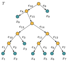
Figure 3: A rooted $X$-tree $T$ for $X=\{x_{1},x_{2},\dots,x_{9}\}.$

Let $s\in\mathcal{P}(T,\ell)$. Without loss of generality we assume $s\in\text{ext}(T,\ell)$. For $j\in\{1,\dots,d_{\hat{T}}\}$ and some $e\in E_{f}$, observe that $s^{j}-s^{0}$ encodes an increase of $s_{j}^{0}$ with $x^{e}=x_{j}$ and possibly a decrease of some score $s_{k}^{0}>\,\text{LB}(x_{k},T)$. Recall that $\gamma(x_{j},e)=0$ for diversity index $\varphi_{\hat{T}}^{0}$. Hence, any choice of a positive value for $\gamma(x_{j},e)$ properly fits our definition of $s^{j}$. This means, for $e\in E_{f}$, $j\in\{1,\dots,d_{\hat{T}}\}$, the free choice of $\gamma(x_{j},e)$, while fixing the rest of $\Gamma_{T}$ to yield the values of $s^{0}$, fully specifies the score $s^{j}$. Therefore, we conclude that making appropriate free choices for all $\gamma(x^{e},e)$, $e\in E_{f}$, yields $s=\sum_{j=1}^{d_{\hat{T}}}s^{j}-(d_{\hat{T}}-1)s^{0}$. This means, $B(x_{i})$ is a maximal linearly independent subset of $\mathcal{P}(T,\ell)$. Thus, we conclude that dim$(T,\ell)=d_{\hat{T}}$.

Now, we have constructed a basis $B(x_{i})$ for the affine hull of $\mathcal{P}(T,\ell)$. However, this affine subspace does not include the null vector. Hence, any vector space that includes $\mathcal{P}(T,\ell)$ has to have dimension greater than dim$(T,\ell)$. Now, taking the linear span of $B(x_{i})$ gives us a basis for the desired vector space with dimension dim$(T,\ell)+1$. Thus, our claim follows.

We call any basis $B(x_{i})\subset\,\text{ext}(T,\ell)$ of the vector space of minimal dimension that includes $\mathcal{P}(T,\ell)$ which has the same form as constructed in Proposition 3.9.1 a canonical basis and we denote the set of canonical bases by $\mathcal{B}(T,\ell)$. We illustrate the construction of a canonical basis in the following example:

Example 5.

Consider the rooted $X$-tree $T$ in Figure 3 and any edge length function $\ell$ on $E(T)$. Let $\varphi_{(T,\ell)}$ be a diversity index. We have $\mathcal{F}(T)=\{\{e_{13},e_{15},e_{16}\}\}$ and therefore $d_{(T,\ell)}=3$. Then, for $x_{i}=x_{1}$, Proposition 3.2 yields the bijection $\phi:\{e_{13},e_{15},e_{16}\}\to\{x_{3},x_{4},x_{8}\}$ with $\phi(e_{13})=x_{3}$, $\phi(e_{15})=x_{4}$ and $\phi(e_{16})=x_{8}$. Based on these observations, let $B(x_{1})=\{s^{0},s^{1},s^{2},s^{3}\}\in\mathcal{B}(T,\ell)$. Then, for $i\in\{1,2\}$, $\gamma(x_{i},e)=1/2$ with $e\in\{e_{13},e_{15},e_{16}\}$ defines $s^{0}$. Furthermore, $\gamma(x_{3},e_{13})=1$ defines $s^{1}-s^{0}$, $\gamma(x_{4},e_{15})=1/4$ defines $s^{2}-s^{0}$ and $\gamma(x_{8},e_{16})=1$ defines $s^{3}-s^{0}$.

Notice that in the proof of Proposition 3.9.1 and Example 5 we have associated a set of independent edges

$$E_{B(x_{i})}\in\{E_{f}\,:\,|P(x_{i})\cap E_{f}|\,\text{maximum},\,E_{f}\in\mathcal{F}(T)\}$$

with each canonical basis $B(x_{i})\in\mathcal{B}(T,\ell)$. This leads to the following exchange property of canonical bases:

Corollary 3.11.

Let $\hat{T}=(T,\ell)$ be a phylogenetic $X$-tree with $d_{\hat{T}}\geq 1$, $x_{i}\in X$, $B(x_{i})=\left\{s^{0},s^{1},\dots,s^{d_{\hat{T}}}\right\}\in\mathcal{B}(T,\ell)$. Then, there exists $j\in\left\{1,\dots,d_{\hat{T}}+1\right\}$, $j\neq i$, such that interchanging the role of $x_{j}$ and $x_{i}$ in $B(x_{i})$ yields another basis $B(x_{j})=\left\{t^{0},t^{1},\dots,t^{d_{\hat{T}}}\right\}\in\mathcal{B}(T,\ell)$ with $t_{i}^{0}=\,\text{LB}(x_{i},T)$.

Proof 3.12.

Let $(u,v)=\,\text{arg\,max}\left\{|P(e)\cap P(x_{i})|\,:\,e\in E_{B(x_{i})}\right\}$ and let $x_{j}=x^{(u,v)}$. By definition of $x^{(u,v)}$ we know that $x_{j}\neq x_{i}$. From Proposition 3.9.1 we obtain a basis $B(x_{j})=\left\{t^{0},t^{1},\dots,t^{d_{\hat{T}}}\right\}\in\mathcal{B}(T,\ell)$. By our choice of $x_{j}$ we deduce that $x_{i}$ satisfies one of the equations (10) for $t^{0}$. Hence, $x_{i}$ attains its minimum allocation from $T$ in $t^{0}$.

In addition, Example 5 illustrates that the construction of a canonical basis necessitates the existence of the bijection in Propositions 3.2. This leads us to combine Propositions 3.2, 3.4 and 3.9 to associate each canonical basis with a valid description of $\mathcal{P}(T,\ell)$:

Corollary 3.13.

Let $\hat{T}=(T,\ell)$ be a rooted phylogenetic $X$-tree with $d_{\hat{T}}\geq 1$, let $x_{i}\in X$, $B(x_{i})\in\mathcal{B}(T,\ell)$ and let $Y\subseteq X$ be the taxa associated with the first $d_{\hat{T}}+1$ coordinates in $B(x_{i})$. Then, there exists $x_{k}\in Y$, $k\neq i$, such that

$$\text{proj}_{Y\setminus\{x_{k}\}}(T,\ell)\subseteq\bigcap_{Z\subseteq Y\setminus\{x_{k}\},\,x_{i}\in Z}\mathcal{S}(x_{k},Y,Z)$$

for

$$\mathcal{S}(x_{k},Y,Z)=\left\{a\in\mathbb{R}_{\geq 0}^{Y\setminus\{x_{k}\}}\,:\,\sum_{x_{j}\in Z}a_{j}\leq r_{i}\left(T(Z),E_{B(x_{i})}\right)-\sum_{x_{j}\in Z}\text{LB}\left(x_{j},Y,T\right)\right\}.$$

Proof 3.14.

From Proposition 3.9.1 we know that sets $E_{B(x_{i})}$ and $Y\setminus\{x_{i}\}$ fit into Proposition 3.2 as sets $E_{f}$ and $Y$, respectively. Hence,

(13) $$r\left(T(Y),E_{B(x_{i})}\right)=r_{i}\left(T(Y),E_{B(x_{i})}\right)-\sum_{x_{j}\in Y}\text{LB}\left(x_{j},Y,T\right).$$

Moreover, we obtain a bijective map $\phi:E_{B(x_{i})}\to Y\setminus\{x_{i}\}$ with $e\in P(\phi(e))$ for all $e\in E_{B(x_{i})}$ from Proposition 3.2. First, this means a free choice of numbers $\gamma(\phi(e),e)$ does fully specify the corresponding matrix $\Gamma_{T}$ of a diversity index. Then, since $|P(x_{i})\cap E_{B(x_{i})}|$ is maximum in $\mathcal{F}(T)$ by definition of $E_{B(x_{i})}$, there exists a bijective map $\phi^{\prime}:E_{B(x_{i})}\to Y\setminus\{x_{k}\}$ for some $x_{k}\in Y$, $k\neq i$, such that a free choice of numbers $\gamma(\phi^{\prime}(e),e)$ does fully specify $\Gamma_{T}$. Therefore, Proposition 3.4 yields

$$\text{proj}_{Y\setminus\{x_{k}\}}(T,\ell)\subseteq\left\{a\in\mathbb{R}_{\geq 0}^{Y\setminus\{x_{k}\}}\,:\,\sum_{x_{j}\in Z}a_{j}\leq r\left(T(Z),E_{B(x_{i})}\right)~{}~{}~{}\forall\,Z\subseteq Y\setminus\{x_{k}\}\right\}.$$

Secondly, we can restrict bijection $\phi$ to have a domain and co-domain of size $d_{\hat{T}}-1$ by removing leaf $x_{k}$ from $T$ and all taxa which share a neutrality condition with respect to edge $\phi^{-1}(x_{k})$. Let $T^{\prime}$ denote the resulting $X^{\prime}$-tree (up to edge subdivisions) for which $X\cap X^{\prime}$ is the set of taxa appearing in both $T$ and $T^{\prime}$. By construction $d_{(T^{\prime},\ell)}=d_{\hat{T}}-1$, and therefore $(T^{\prime},\ell)$, $E_{B(x_{i})}\setminus\left\{\phi^{-1}(x_{k})\right\}$ and $Y\setminus\{x_{i},x_{k}\}$ fit into Proposition 3.2 as $\hat{T}$, $E_{f}$ and $Y$, respectively. Since $T^{\prime}(Y\setminus\{x_{k}\})=T(Y\setminus\{x_{k}\})$, we can conclude from further restrictions of bijection $\phi$ that equation (13) holds for all $Z\subseteq Y$ with $x_{i}\in Z$. Thus, our claim follows.

We will use Corollary 3.13 to study a proper projection of $\mathcal{P}(T,\ell)$ for which Proposition 3.9 enables us to assess all independence relations.

3.3 All facets of the diversity index polytope

For $Y\subseteq X$ and $x_{k}\in Y$, let $\mathcal{Z}(x_{k},Y)$ denote the subsets $Z\subseteq Y\setminus\{x_{k}\}$ such that $Y\setminus Z$ are in the same connected component of $F(Y-Z)$. Now, we can provide the facets of $\mathcal{P}(T,\ell)$:

Theorem 3.15.

Let $\hat{T}=(T,\ell)$ be a rooted phylogenetic $X$-tree with $d_{\hat{T}}\geq 1$. Then, for $s\in\mathcal{P}(T,\ell)$,

1. the inequalities

   (14) $$s_{i} \geq\,\text{LB}(x_{i},T)~{} \forall\,i\in\{1,\dots,n\}$$

   are facet-defining for $\mathcal{P}(T,\ell)$.

2. $x_{i}\in X$, $B(x_{i})\in\mathcal{B}(T,\ell)$ and $Y\subseteq X$ the taxa associated with the first $d_{\hat{T}}+1$ coordinates in $B(x_{i})$, there exists $x_{k}\in Y$, $k\neq i$, such that the inequalities

   (15) $$\sum_{x_{j}\in Z}N(x_{j})\cdot\left(s_{j}-\,\text{LB}\left(x_{j},T\right)\right)\leq r\left(T(Z),E_{B(x_{i})}\right)$$

   for all $Z\in\mathcal{Z}(x_{k},Y)$ with $x_{i}\in Z$ are facet-defining for $\mathcal{P}(T,\ell)$.

Proof 3.16.

1.: By definition we know that inequalities (14) are valid. For $x_{i}\in X$, let $B(x_{i})=\left\{s^{0},s^{1},\dots,s^{d_{\hat{T}}}\right\}\in\mathcal{B}(T,\ell)$. Then, we know from Corollary 3.11 that there exists a basis $B(x_{j})=\left\{t^{0},t^{1},\dots,t^{d_{\hat{T}}}\right\}\in\mathcal{B}(T,\ell)$ with $t_{i}^{0}=\text{LB}(x_{i},T)$. By definition of $B(x_{j})$ (see Proposition 3.9.1), we have

$$t_{l}^{0} \geq t_{l}^{k},~{}t_{k}^{k}>t_{l}^{k}~{} \forall\,l\in\{1,\dots,d_{\hat{T}}+1\},k\in\{1,\dots,j-1\},l\neq k,$$

$$t_{l}^{0} \geq t_{l}^{k},~{}t_{k+1}^{k}>t_{l}^{k}~{} \forall\,l\in\{1,\dots,d_{\hat{T}}+1\},k\in\{j,\dots,d_{\hat{T}}\},l\neq k+1.$$

Hence, $\text{LB}(x_{i},T)=t_{i}^{0}\geq t_{i}^{k}$ for all $k\in\{1,\dots,j-1\},i\neq k$ and $k\in\{j,\dots,d_{\hat{T}}\},i\neq k+1$. This means, $x_{i}$ attains a score of LB$(x_{i},T)$ in exactly $d_{\hat{T}}$ elements of $B(x_{j})$. In other words, there exists a subset $B_{i}\subset B(x_{j})$ of $d_{\hat{T}}$ linearly independent vectors with a score of LB$(x_{i},T)$ for $x_{i}$ in every element of $B_{i}$. This means, $B_{i}$ constitutes a set of $(d_{\hat{T}}-1)$ affinely independent vectors satisfying (14) with equality. Thus, inequalities (14) are facet-defining.
 
2.: From Corollary 3.13 we know that there exists $x_{k}\in Y$, $k\neq i$, such that inequalities (15) are valid for all $Z\subseteq Y\setminus\{x_{k}\}$ with $x_{i}\in Z$. Moreover,

(16) $$r\left(T(Z),E_{B(x_{i})}\right)=r_{i}\left(T(Z),E_{B(x_{i})}\right)-\sum_{x_{i}\in Z}\text{LB}(x_{i},Y,T).$$

We prove our claim by induction on the recursion depth $\delta$ of formula (6) for $x_{i}$. Let $Z\in\mathcal{Z}(x_{k},Y)$ with $x_{i}\in Z$. Let $Z_{j}$ denote the leafset of $T_{j}(Z-x_{i})$ and let $E_{f}=E_{B(x_{i})}$.

Let $\delta=0$: Then, $I\left(x_{i},Z,E_{f}\right)=\emptyset$. This means, there exist no taxon $x_{j}$ with $P(x_{j})\cap E_{f}\neq\emptyset$ which is present in $F(Z-x_{i})$. This leads to a contradiction because $d_{\hat{T}}\geq 1$ implies $E_{f}\neq\emptyset$. Therefore, $\delta=0$ cannot occur.

Let $\delta=1$: By definition (6),

$$r_{i}\left(T(Z),E_{f}\right)$$

$$=\sum_{e\in\mathcal{E}^{*}(x_{i},E_{f},E_{f},Y\setminus Z)}N(x_{i},e,Y)\cdot\ell(e)+\sum_{x_{j}\in\mathcal{I}\left(x_{i},Z,E_{f}\right)}r_{j}\left(T_{j}(Z-x_{i}),E_{f|i}\right)$$

Since $\delta=1$, for $x_{j}\in\mathcal{I}\left(x_{i},Z,E_{f}\right)$, we have $\mathcal{I}\left(x_{j},Z,E_{f}\right)=\emptyset$. This means, $T_{j}(Z-x_{i})$ does not contain any edges from $E_{f}$. Hence, $E_{f|i}=\emptyset$ and no paths in $T$ outside $T_{j}(Z-x_{i})$ contain independent edges in the same equivalence class as independent edges in $T_{j}(Z-x_{i})$. Equivalently, $\mathcal{E}(x_{j},E_{f|i},E_{f},Y\setminus Z_{j})=\emptyset$. Thus, we conclude

$$r_{j}\left(T_{j}(Z-x_{i}),E_{f|i}\right) =\,\text{LB}(x_{j},Y,T)~{} \forall\,x_{j}\in\mathcal{I}\left(x_{i},Z,E_{f}\right).$$

This means, for $x_{j}\in Z$ we have $\hat{X}_{x_{j},e}=\hat{X}_{x_{j}}$ for all $e\in E_{f}$. Therefore, since $x_{i}\in Y$,

$$N(x_{i},e,Y)=\left|\hat{X}_{x_{i},e}\cap\bigcup_{y\in Y}\hat{X}_{y}\right|/\left|\hat{X}_{x_{i},e}\right|=1.$$

Hence,

$$r_{i}\left(T(Z),E_{f}\right) =\sum_{e\in\mathcal{E}^{*}(x_{i},E_{f},E_{f},Y\setminus Z)}\ell(e)+\sum_{x_{j}\in\mathcal{I}\left(x_{i},Z,E_{f}\right)}\text{LB}(x_{j},Y,T)$$

(17) $$=N(x_{i})\cdot\left[\text{UB}(x_{i},T)-\,\text{LB}(x_{i},T)\right]+\sum_{x_{j}\in Z}\text{LB}(x_{j},Y,T).$$

Next, we can apply Lemma 3.6 for $x_{j},x_{k}\in Z$, $j\neq k$, to get

(18) $$N(x_{j})\cdot R\left(x_{j},x_{k},E_{f}\right)=N(x_{k})\cdot R\left(x_{k},x_{j},E_{f}\right).$$

In addition, for $B(x_{i})=\left\{s^{0},s^{1},\dots,s^{d_{\hat{T}}}\right\}$ we know from Proposition 3.9.1 that

$$s_{i}^{0} =\,\text{UB}\left(x_{i},T\right),$$

$$s_{i}^{h} =\,\text{UB}\left(x_{i},T\right)-R\left(x_{i},x_{h},E_{f}\right)~{}~{}\forall\,h\in\{1,\dots,i-1\},$$

$$s_{i}^{h} =\,\text{UB}\left(x_{i},T\right)-R\left(x_{i},x_{h+1},E_{f}\right)~{}~{}\forall\,h\in\{i,\dots,d_{\hat{T}}\}.$$

Hence, from (16) and (17) we deduce that

$$r\left(T(Z),E_{f}\right) =N(x_{i})\cdot\left[\text{UB}(x_{i},T)-\,\text{LB}(x_{i},T)\right]$$

(19) $$=\sum_{x_{j}\in Z}N(x_{j})\cdot\left(s_{j}^{0}-\,\text{LB}(x_{j},T)\right).$$

Let $h\in\left\{1,\dots,d_{\hat{T}}\right\}$. Without loss of generality $h\in\{1,\dots,i-1\}$. We have

$$N(x_{i})\cdot\left(s_{i}^{h}-\,\text{LB}(x_{i},T)\right) =N(x_{i})\cdot\left(\text{UB}(x_{i},T)-\,\text{LB}(x_{i},T)-R\left(x_{i},x_{h},E_{f}\right)\right)$$

$$=N(x_{i})\cdot\left(s_{i}^{0}-\,\text{LB}(x_{i},T)\right)-N(x_{i})\cdot R\left(x_{i},x_{h},E_{f}\right).$$

The same arguments apply when we reverse the role of $i$ and $h$. Hence, using (18) we infer that

$$N(x_{i})\cdot\left(s_{i}^{h}-\,\text{LB}(x_{i},T)\right)+N(x_{h})\cdot\left(s_{h}^{h}-\,\text{LB}(x_{h},T)\right)$$

$$=\, N(x_{i})\cdot\left(s_{i}^{0}-\,\text{LB}(x_{i},T)\right)+N(x_{h})\cdot\left(s_{h}^{0}-\,\text{LB}(x_{h},T)\right).$$

In addition, for $j\in\{1,\dots,d_{\hat{T}}+1\}$, $i\neq j\neq h$, we have $s_{j}^{h}=s_{j}^{0}$ because

$$\text{LB}(x_{j},T)=s_{j}^{0}\geq s_{j}^{h}$$

follows from Proposition 3.9.1. Thus,

$$\sum_{x_{j}\in Z}s_{j}^{0} =\sum_{x_{j}\in Z}s_{j}^{h}~{} \forall\,h\in\left\{1,\dots,d_{\hat{T}}\right\},~{}h\neq k.$$

In other words, equation (19) holds for $s^{0}$ and $d_{\hat{T}}-1$ pairwise distinct vectors from $\left\{s^{h}\,:\,h\in\{1,\dots,d_{\hat{T}}\}\right\}$. Thus, $d_{\hat{T}}$ vectors from $B(x_{i})$ satisfy inequality (15) with equality. Moreover, every connected component of $F(Z-x_{i})$ contains at most one taxon from $Z$. Therefore, taxa $Y\setminus Z$ are in the same connected component of $F(Y-Z)$, i.e., $Z\in\mathcal{Z}(x_{k},Y)$, if and only if $|Z|=d_{\hat{T}}$. Thus, inequality (15) is facet-defining for $\mathcal{P}(T,\ell)$.

$\delta\to\delta+1$: Without loss of generality $\mathcal{I}\left(x_{i},Z,E_{f}\right)=\left\{x_{1},\dots,x_{d}\right\}$ with $d\leq|Z|-1$ and $x_{j}=\text{argmax}~{}r\left(T_{j}(Z-x_{i}),E_{f|i}\right)$ for all $j\in\{1,\dots,d\}$. Then, by our induction hypothesis there exist $|Z_{j}|$ linearly independent vectors $A(x_{j})=\left\{s^{j,0},\dots,s^{j,|Z_{j}|-1}\right\}\subset B(x_{j})$ for some basis $B(x_{j})=\left\{s^{j,0},\dots,s^{j,d_{j}}\right\}\in\mathcal{B}\left(T_{j}(Z-x_{i}),\ell\right)$, $d_{j}=d_{(T_{j}(Z-x_{i}),\ell)}$, such that

(20) $$\sum_{x_{l}\in Z_{j}}N(x_{l})\cdot\left(s_{l}-\,\text{LB}(x_{l},T)\right) =r\left(T_{j}(Z-x_{i}),E_{f|i}\right)~{} \forall\,s\in A(x_{j}).$$

Consider $B(x_{i})=\left\{s^{0},s^{1},\dots,s^{d_{\hat{T}}}\right\}\in\mathcal{B}(T,\ell)$ and denote the edge $\hat{e}$ defined by taxa $x=x_{i}$ and $y=x_{j}$ in Lemma 3.6 by $\hat{e}(i,j)$. Then, define a set of vectors

$$\mathcal{S}(Z)=\bigcup_{j=1}^{d}\left\{t^{j,0},\dots,t^{j,|Z_{j}|-1}\right\}\cup\{s^{0}\}\subset\mathcal{P}(T,\ell)$$

by setting, for $j\in\{1,\dots,d\}$, $t^{j,0}=s^{0}$ except for

$$t^{j,0}_{l} =s_{l}^{0}-R\left(x_{i},x_{j},E_{f}\right)~{} \forall\,x_{l}\in\hat{X}_{x_{i},\hat{e}(i,j)}\cap Z,$$

$$t^{j,0}_{l} =s_{l}^{0}+R\left(x_{j},x_{i},E_{f}\right)~{} \forall\,x_{l}\in\hat{X}_{x_{j},\hat{e}(i,j)}\cap Z$$

and, for $j\in\{1,\dots,d\}$, $l\in\{1,\dots,|Z_{j}|-1\}$, $t^{j,l}=s^{0}$ except for

$$t_{p}^{j,l} =s_{p}^{j,l}~{} \forall\,x_{p}\in Z_{j}.$$

By definition, $s^{0}$ equals $s^{j,0}$ when constrained to the pendant subtree $T_{j}(Z-x_{i})$. Hence, analogously as for our induction base $\delta=1$ (see equation (19)), we know from (20) and Proposition 3.9.1 that

$$\sum_{x_{j}\in Z}N(x_{j})\cdot\left(s_{j}^{0}-\,\text{LB}(x_{j},T)\right)=r_{i}\left(T(Z),E_{f}\right)-\,\sum_{x_{j}\in Z}\text{LB}(x_{j},Y,T).$$

For $j\in\{1,\dots,d\}$, we have

$$\sum_{x_{l}\in Z}N(x_{l})\cdot t^{j,0}_{l}-\sum_{x_{l}\in Z}N(x_{l})\cdot s^{0}_{l}$$

$$=\sum_{x_{l}\in\hat{X}_{x_{j},\hat{e}(i,j)}\cap Z}N(x_{l})\cdot R\left(x_{j},x_{i},E_{f}\right)-\sum_{x_{l}\in\hat{X}_{x_{i},\hat{e}(i,j)}\cap Z}N(x_{l})\cdot R\left(x_{i},x_{j},E_{f}\right)$$

$$=\left|\hat{X}_{x_{j},\hat{e}(i,j)}\right|\cdot R\left(x_{j},x_{i},E_{f}\right)-\left|\hat{X}_{x_{i},\hat{e}(i,j)}\right|\cdot R\left(x_{i},x_{j},E_{f}\right)=0$$

where the second and third equality follow from our choice of $Y$ and Lemma 3.6, respectively. Furthermore, for $l\in\{1,\dots,|Z_{j}|-1\}$,

$$\sum_{x_{p}\in Z}N(x_{p})\cdot\left(t^{j,l}_{p}-\,\text{LB}(x_{p},T)\right)$$

$$=\sum_{x_{p}\in Z\setminus Z_{j}}N(x_{p})\cdot\left(s^{0}_{p}-\,\text{LB}(x_{p},T)\right)+\sum_{x_{p}\in Z_{j}}N(x_{p})\cdot\left(s^{j,l}_{p}-\,\text{LB}(x_{p},T)\right)$$

$$\begin{subarray}{c}\eqref{eq::IHj}\\ =\end{subarray}\sum_{x_{p}\in Z\setminus Z_{j}}N(x_{p})\cdot\left(s^{0}_{p}-\,\text{LB}(x_{p},T)\right)+r\left(T_{j}(Z-x_{i}),E_{f|i}\right)$$

$$\stackrel{{\scriptstyle\text{Proposition}~{}\ref{prop::basis}.1}}{{=}}r_{i}\left(T(Z),E_{f}\right)-\,\sum_{x_{j}\in Z}\text{LB}(x_{j},Y,T).$$

Thus, all vectors in $\mathcal{S}(Z)$ satisfy inequality (15) with equality. Next, we will show that $\mathcal{S}(Z)$ is a set of linearly independent vectors and subsequently show how to extend the set $\mathcal{S}(Z)$ to a set of $d_{\hat{T}}$ linearly independent vectors satisfying inequality (15) with equality.

For $j\in\{1,\dots,d\}$, observe that the set $B_{j}=\left\{t^{j,0},\dots,t^{j,|Z_{j}|-1}\right\}$, when restricted to taxa in $Z_{j}$, differs from $A(x_{j})=\left\{s^{j,0},\dots,s^{j,|Z_{j}|-1}\right\}$ only in the fact that $t_{l}^{j,0}=s_{l}^{j,0}+R(x_{j},x_{i},E_{f})$ for all $x_{l}\in\hat{X}_{x_{j},\hat{e}(i,j)}$. Recall that $s^{j,0}$ is the image of the diversity index defined by the allocation of edges in the calculation of $r(T_{j}(Z-x_{i}),E_{f|i})$. This means, $s_{l}^{j,0}$ is maximum with respect to diversity scores of taxon $x_{l}\in\hat{X}_{x_{j},\hat{e}(i,j)}$ in $\mathcal{P}\left(T_{j}(Z-x_{i}),\ell\right)$. Using the maximality of $s_{l}^{j,0}$ we conclude that the restriction of $B_{j}$ to $Z_{j}$ has the same linear independence relations as $A(x_{j})$. Moreover, for $h\in\{1,\dots,d\}$, $h\neq j$, $B_{h}$ restricted to taxa in $Z_{j}$ yields $|Z_{h}|$ copies of $s^{0}$ restricted to $Z_{j}$. In addition, the restriction of $s^{0}$ to taxa in $Z_{j}$ equals $s^{j,0}$ by definition of bases $B(x_{i})$ and $B(x_{j})$, and $t^{h,0}$ and $t^{j,0}$ are linear independent by construction. This means, $B_{h}\cup B_{j}$ is a set of linearly independent vectors. Thus, $\mathcal{S}(Z)\setminus\{s^{0}\}$ is a set of linearly independent vectors. Furthermore, $s^{0}$ is linearly independent from vectors $t^{1,0},\dots,t^{d,0}$ by construction. For $j\in\{1,\dots,d\}$, since the restriction of $s^{0}$ to taxa in $Z_{j}$ equals $s^{j,0}$, we know that $\{s^{0}\}\cup B_{j}\setminus\{t^{j,0}\}$ is a set of linearly independent vectors. Hence, we conclude that $B_{j}\cup\{s^{0}\}$ is a set of linearly independent vectors. Thus, in total we conclude that $\mathcal{S}(Z)$ is a set of

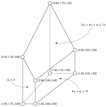
Figure 4: The diversity index polytope $\mathcal{P}(T,\ell)$ for the rooted $X$-tree $T$ in Figure 3 and edge length function $\ell:E(T)\to\mathbb{R}_{\geq 0}$ with $\ell(e)=1$ such that diversity index scores $s\in\mathcal{P}(T,\ell)$ are projected onto vectors $(s_{1},s_{4},s_{8})$ (using the fact that dim$(T,\ell)=d_{(T,\ell)}=3$). The polytope $\mathcal{P}(T,\ell)$ can be described by $6$ facets, $3$ of the form (14) and $3$ of the form (15).

$$1+\sum_{j=1}^{d}|Z_{j}|=|Z|$$

linearly independent vectors. Since $Y\setminus Z$ are in the same connected component of $F(Y-Z)$, for $Z_{d+1}=Y\setminus Z$ and $x_{d+1}\in Z_{d+1}$, there exists a set of $|Z_{d+1}|$ linearly independent vectors

$$A(x_{d+1})=\left\{s^{d+1,0},\dots,s^{d+1,|Z_{d+1}|-1}\right\}\subset B(x_{d+1})\in\mathcal{B}\left(T_{d+1}(Z-x_{i}),\ell\right).$$

For $l\in\{1,\dots,|Z_{d+1}|-1\}$, set $t^{d+1,l}=s^{0}$ except for

$$t_{p}^{d+1,l} =s_{p}^{d+1,l}~{} \forall\,x_{p}\in Y\setminus Z.$$

Then, $\mathcal{S}(Z)\cup\left\{t^{d+1,1},\dots,t^{d+1,|Z_{d+1}|-1}\right\}$ is a set of $|Z|+|Y\setminus Z|-1=d_{\hat{T}}$ linearly independent vectors that satisfy inequality (15) with equality. Thus, our claim follows.

We illustrate Theorem 3.15 in Figure 4. Specifically, the following example details facets of form (15):

Example 6.

Consider the rooted phylogenetic $X$-tree $(T,\ell)$ in Figure 3. As observed in Example 5, $d_{\hat{T}}=3$ and $E_{f}=\{e_{13},e_{15},e_{16}\}$ is the only set of independent edges for $T$. Hence, $Y=\{x_{1},x_{3},x_{4},x_{8}\}$ is one possible choice for the first $d_{\hat{T}}+1=4$ coordinates in $B(x_{1})$ (another possible choice could be $Y=\{x_{1},x_{3},x_{7},x_{8}\}$). Observe that $N(x_{3})=N(x_{8})=1$, $N(x_{1})=2$ and $N(x_{4})=4$, and that $x_{k}=x_{3}$ is the taxon which fits into Corollary 3.13 (and therefore fits into Theorem 3.15.2). Let $Z=\{x_{1},x_{4},x_{8}\}\in\mathcal{Z}(x_{3},Y)$. Then, we have

$$r\left(T(Z),E_{f}\right)=r_{1}\left(T(Z),E_{f}\right)-\sum_{x_{j}\in Z}\text{LB}\left(x_{j},Y,T\right)=\ell(e_{13})+\ell(e_{15})+\ell(e_{16})=3.$$

Hence, we know from Theorem 3.15.2 that

$$\sum_{x_{j}\in Z}N(x_{j})\cdot\left(s_{j}-\,\text{LB}(x_{j},T)\right)=2(s_{1}-1.5)+4(s_{4}-1.75)+s_{8}-1 \leq r\left(T(Z),E_{f}\right)$$

$$\Leftrightarrow~{}~{}~{}2s_{1}+4s_{4}+s_{8} \leq 14$$

is a facet of $\mathcal{P}(T,\ell)$. Next, consider $Y$ as the first four coordinates in $B(x_{4})$. Then, $x_{k}\in\{x_{1},x_{3}\}$ fits into Corollary 3.13. Hence, for $Z=\{x_{4},x_{8}\}\in\mathcal{Z}(x_{k},Y)$, we have $r\left(T(Z),E_{f}\right)=r_{4}\left(T(Z),E_{f}\right)-\sum_{x_{j}\in Z}\text{LB}\left(x_{j},Y,T\right)=\ell(e_{15})+\ell(e_{16})=2$ and therefore Theorem 3.15.2 yields facet

$$\sum_{x_{j}\in Z}N(x_{j})\cdot\left(s_{j}-\,\text{LB}(x_{j},T)\right)=4(s_{4}-1.75)+s_{8}-1 \leq r\left(T(Z),E_{f}\right)$$

$$\Leftrightarrow~{}~{}~{}4s_{4}+s_{8} \leq 10$$

If instead we choose $Z=\{x_{1},x_{4}\}\notin\mathcal{Z}(x_{k},Y)$, then Theorem 3.15.2 is not applicable but we know from Corollary 3.13 that

$$r\left(T(Z),E_{f}\right)=r_{4}\left(T(Z),E_{f}\right)-\sum_{x_{j}\in Z}\text{LB}\left(x_{j},Y,T\right)=\ell(e_{13})+\ell(e_{15})+\ell(e_{16})=3$$

and inequality

$$\sum_{x_{j}\in\{x_{1},x_{4}\}}N(x_{j})\cdot\left(s_{j}-\,\text{LB}(x_{j},T)\right)=2(s_{1}-1.5)+4(s_{4}-1.75) \leq r\left(T(Z),E_{f}\right)$$

(21) $$\Leftrightarrow~{}~{}~{}2s_{1}+4s_{4} \leq 13$$

is valid. Indeed, inequality (21) is not a facet because $2s_{1}+4s_{4}=13$ is the intersection of facets $2s_{1}+4s_{4}+s_{8}=14$ and $s_{8}=\,\text{LB}(x_{8},T)=1$ (see Theorem 3.15.1). Lastly, consider $Y$ as the first four coordinates in $B(x_{8})$. Then, $x_{k}\in Y\setminus\{x_{8}\}$ fits into Corollary 3.13. Hence, for $Z=\{x_{8}\}\in\mathcal{Z}(x_{k},Y)$, we have $r\left(T(Z),E_{f}\right)=r_{8}\left(T(Z),E_{f}\right)-\sum_{x_{j}\in Z}\text{LB}\left(x_{j},Y,T\right)=\ell(e_{16})=1$ and therefore Theorem 3.15.2 yields

$$\sum_{x_{j}\in Z}N(x_{j})\cdot\left(s_{j}-\,\text{LB}(x_{j},T)\right)=s_{8}-1 \leq r\left(T(Z),E_{f}\right)~{}~{}~{}\Leftrightarrow~{}~{}~{}s_{8}\leq 2.$$

Figure 4 illustrates the three facets from this example. The plane described by equation (21) intersects with $\mathcal{P}(T,\ell)$ only in points $\alpha(3,1.75,1)+(1-\alpha)(2,2.25,1)$ for $\alpha\in[0,1]$.

We can generalize our observations in Example 6 to prove that Theorem 3.15 gives a characterization of all facets of $\mathcal{P}(T,\ell)$. To this end, let $\mathcal{Z}(T,\ell)$ denote the set of subsets $Z\in\mathcal{Z}(x_{k},Y)$, $x_{i}\in Z$, for which Theorem 3.15.2 is applicable.

Theorem 3.17.

Let $\hat{T}=(T,\ell)$ be a rooted phylogenetic $X$-tree with $d_{\hat{T}}\geq 1$. Then, there exist $n+|\mathcal{Z}(T,\ell)|$ linear inequalities which constitute a minimal compact description of the polytope $\mathcal{P}(T,\ell)$.

Proof 3.18.

First observe that the union of the descriptions of all projections of $\mathcal{P}(T,\ell)$ to $d_{\hat{T}}$ taxa in Corollary 3.13 contains all facets of $\mathcal{P}(T,\ell)$. Hence, for all $Z\subseteq Y\setminus\{x_{k}\}$, $x_{i}\in Z$, we need to prove or disprove that the inequalities in Corollary 3.13 are facet-defining for $\mathcal{P}(T,\ell)$. Theorem 3.15.1 proves that the non-negativity constraints of the projected diversity index scores are facet-defining. In addition, if $Z\in\mathcal{Z}(x_{k},Y)$, $x_{i}\in Z$, then we obtain facet-defining inequalities (15) from Theorem 3.15.2. Otherwise, $Z\notin\mathcal{Z}(x_{k},Y)$, $x_{i}\in Z$, for any choice of $x_{k}$ which fits into Corollary 3.13. In this case we show that

(22) $$\sum_{x_{j}\in Z}N(x_{j})\cdot\left(s_{j}-\,\text{LB}(x_{j},T)\right)\leq r\left(T(Z),E_{B(x_{i})}\right)$$

is not facet-defining for $\mathcal{P}(T,\ell)$. Let $W_{k}\subset Y\setminus Z$ be the taxa which are in the same connected component of $F(Y-Z)$ as $x_{k}$. Then, $Y\setminus W_{k}\in\mathcal{Z}(x_{k},Y)$. Hence, we know from Theorem 3.15.2 that inequality

(23) $$\sum_{x_{j}\in Y\setminus W_{k}}N(x_{j})\cdot\left(s_{j}-\,\text{LB}(x_{j},T)\right)\leq r\left(T(Y\setminus W_{k}),E_{B(x_{i})}\right)$$

is facet-defining for $\mathcal{P}(T,\ell)$. Furthermore, taxa $Y\setminus(Z\cup W_{k})$ are the taxa in the connected components of $F(Y-Z)$ different from $W_{k}$. Let $X_{1},\dots,X_{p}$ denote the taxa present in these components, i.e., $\bigcup_{j=1}^{p}X_{j}=Y\setminus(Z\cup W_{k})$. For $j\in\{1,\dots,p\}$, let $T_{j}$ denote the connected component in $F(Y-Z)$ with leafset $X_{j}$. If $\mathcal{F}(T_{j})=\emptyset$, then

(24) $$\sum_{x_{l}\in X_{j}}N(x_{l})\cdot\left(s_{l}-\,\text{LB}(x_{l},T)\right)\leq r\left(T_{j},\emptyset\right)$$

holds with equality, induced by facets (14). Otherwise, we repeat our arguments for $T_{j}$ instead of $T$. Hence, by induction we conclude that inequality (24) is not facet-defining for $\mathcal{P}(T_{j},\ell)$. Furthermore, equation (22) is the intersection of equation (23) and equations (24) for all $j\in\{1,\dots,p\}$. Thus, inequality (22) is not facet-defining for $\mathcal{P}(T,\ell)$.

4 Conclusions and future research

We conclude from Theorem 3.17 that there exists a minimal compact description of the diversity index polytope of polynomial size. So if we characterize a selection criterion for a diversity index by a linear function, then the calculation of the optimal index under this selection criterion can be done in polynomial time by linear programming. We envisage two immediate applications within this framework, though more are likely. Both contain properties of diversity indices for which precise optimal solutions are unknown, but where finding optima would prove useful to conservation planners.

The first concerns the extent to which sets of, say, $k$ species with the largest diversity index scores are able to represent the biodiversity present in the tree as a whole [4, 10]. The separation of these two aspects of biodiversity could be quantified using a linear difference function of distinct measures involving diversity indices as our selection criterion. Taking the perspective of robust optimization [1], diversity indices seen as a region of uncertainty can make this analysis of biodiversity measure differences agnostic to a specific selected set of $k$ species.

The second application involves the way that extinctions of species impact diversity index scores of survivors. The demise of a species results in the removal of that leaf and incident edge from the phylogenetic tree. For example, modelled by a stochastic birth-death process [9]. In doing so, the diversity index scores of remaining leaves are recalculated to reflect the new tree structure. However, this recalculation can lead to quite drastic changes in index scores. Of particular concern, a ranking based on these scores can sometimes become completely reversed after certain extinctions, causing great upset to conservation priorities [6]. Finding optimal diversity indices that best preserve rankings in the presence of extinction events would be a key benefit of the present construction. This problem requires the extension of the diversity index polytope to capture the dependencies between species introduced by a ranking. In this context, approaches like the rotation method introduced by Bolotashvili and Kovalev [2] to study rankings in the linear ordering polytope [3] can inform the study of diversity rankings.

Overall, the results in this articles offer a way of rigorously codifying $\mathcal{P}(T,\ell)$. This opens the door for an analysis of the properties of diversity indices on a broad scale unlike what has previously been attained. In other words, our results introduce the methodological advantages of polyhedral combinatorics to solve problems in conversation biology.

Appendix A Proof of Proposition 3.1

Proof A.1.

By definition, ext$(T,\ell)\subseteq\mathcal{P}(T,\ell)$. If $d_{\hat{T}}=0$, then $|\mathcal{P}(T,\ell)|=1$ and therefore our claim holds. Hence, assume $d_{\hat{T}}\geq 1$. Let $s=\Gamma_{T}l\in\text{ext}(T,\ell)$. Suppose, with a view to contradiction, that $s$ is not an extreme point of $\mathcal{P}(T,\ell)$. Since $\mathcal{P}(T,\ell)$ is convex by Proposition 2.5.2, there exist $\Gamma_{T}^{j}l\in\mathcal{P}(T,\ell)$, $\Gamma_{T}^{j}\neq\Gamma_{T}$, $\lambda_{j}>0$, $j\in\{1,\dots,k\}$, $k\geq 2$, such that

$$\Gamma_{T}l=\sum_{j=1}^{k}\lambda_{j}\Gamma_{T}^{j}l,~{}~{}~{}\sum_{j=1}^{k}\lambda_{j}=1.$$

Hence,

$$\gamma(x_{i},e) =\sum_{j=1}^{k}\lambda_{j}\gamma^{j}(x_{i},e)~{} \forall\,i\in\{1,\dots,n\}.$$

For $e\in E_{f}$, there exists a taxon $x\in X$ such that $\gamma(x,e)=0$. To see this, observe that the minimum value for any free choice in $\Gamma_{T}(e)$ is zero and the maximum value for any free choice of $\gamma(y,e)$, $y\in X$, does imply $\gamma(z,e)=0$ for at least one $z\in X$, $z\neq y$. This means $\sum_{j=1}^{k}\lambda_{j}\gamma^{j}(x,e)=0$. Since $\lambda_{j}>0$ for all $j\in\{1,\dots,n\}$, we obtain $\gamma^{j}(x,e)=0$. Therefore, for $j\in\{1,\dots,n\}$, $\Gamma_{T}(e)=\Gamma_{T}^{j}(e)$. However, for $j\in\{1,\dots,n\}$, we assumed $\Gamma_{T}\neq\Gamma_{T}^{j}$, leading to a contradiction. Thus, $s$ is an extreme point of $\mathcal{P}(T,\ell)$.

Conversely, let $s=\Gamma_{T}l\in\mathcal{P}(T,\ell)\setminus\text{ext}(T,\ell)$. This means, for at least one edge $e\in E_{f}$, no free choice in $\Gamma_{T}(e)$ is maximum or minimum. Let $\Gamma_{T}^{1}l,\Gamma_{T}^{2}l\in\mathcal{P}(T,\ell)$ such that, for some fixed $x\in X$, $\gamma^{1}(x,e)$ and $\gamma^{2}(x,e)$ are given by a maximum and minimum free choice, respectively, and $\Gamma_{T}^{1}(e^{\prime})=\Gamma_{T}^{2}(e^{\prime})=\Gamma_{T}(e^{\prime})$ for all $e^{\prime}\in E(T)\setminus\{e\}$. Hence, for some $\alpha>0$, $\Gamma_{T}(e)=\alpha\Gamma_{T}^{1}(e)+(1-\alpha)\Gamma_{T}^{2}(e)$, meaning $s$ is a convex combination of two diversity index scores which are pairwise distinct from $s$. Thus, $s$ is not an extreme point of $\mathcal{P}(T,\ell)$ because $\mathcal{P}(T,\ell)$ is convex.

Appendix B Proof of Lemma 3.8

Proof B.1.

By induction on $m$. For $m=2$, $a_{1},a_{2},b_{4}>0$, $b_{1},b_{2},b_{3}\geq 0$ and $\lambda\in\mathbb{R}^{2}$, equations

$$(A+B)\lambda=\left[\begin{array}[]{cc}a_{1}+b_{1}&a_{1}-b_{3}\\ a_{2}-b_{2}&a_{2}+b_{4}\end{array}\right]\lambda=0$$

imply

$$\left(a_{2}+b_{4}-\frac{(a_{1}-b_{3})(a_{2}-b_{2})}{a_{1}+b_{1}}\right)\lambda_{2}=0.$$

Hence, either $\lambda_{2}=0$ (and therefore $\lambda_{1}=0$) or $(a_{1}+b_{1})(a_{2}+b_{4})=(a_{1}-b_{3})(a_{2}-b_{2})$. In the latter case, $a_{1}(b_{2}+b_{4})+a_{2}(b_{1}+b_{3})+b_{1}b_{4}=b_{2}b_{3}=0$, leading to a contradiction because $a_{1}b_{4}>0$. Thus, ker$(A+B)=\{(0,0)\}$, i.e., $A+B$ has full rank.

Now, assume our induction hypothesis holds for $m-1$. Without loss of generality we can write

$$A+B=\left[\begin{array}[]{ccccc}a_{1}+b_{1}&a_{1}-b_{3}&a_{1}&\dots&a_{1}\\ a_{2}-b_{2}\\ a_{3}&&\hat{C}\\ \vdots\\ a_{m}\end{array}\right]$$

for a suitable matrices $\hat{A},\hat{B}\in\mathbb{R}^{(m-1)\times(m-1)}$, $\hat{C}=\hat{A}+\hat{B}$ and $a_{1},\dots,a_{m}>0$, $b_{1},b_{2},b_{3}\geq 0$ with $b_{2}b_{3}=0$. Then, for $\lambda\in\mathbb{R}^{m}$, $(A+B)\lambda=0$ can be reformulated as

(30) $$\left[\begin{array}[]{cccc}1&\frac{a_{1}-b_{3}}{a_{1}+b_{1}}&\frac{a_{1}}{a_{1}+b_{1}}&\dots\\ 0&\hat{a}_{11}-\frac{(a_{2}-b_{2})(a_{1}-b_{3})}{a_{1}+b_{1}}+\hat{b}_{11}&\hat{a}_{12}-\frac{(a_{2}-b_{2})a_{1}}{a_{1}+b_{1}}+\hat{b}_{12}&\dots\\ 0&\hat{a}_{21}-\frac{a_{3}(a_{1}-b_{3})}{a_{1}+b_{1}}+\hat{b}_{21}&\hat{a}_{22}-\frac{a_{3}a_{1}}{a_{1}+b_{1}}+\hat{b}_{22}&\dots\\ \vdots&\vdots&&\\ 0&\hat{a}_{(m-1)1}-\frac{a_{m}(a_{1}-b_{3})}{a_{1}+b_{1}}+\hat{b}_{(m-1)1}&\hat{a}_{(m-1)2}-\frac{a_{m}a_{1}}{a_{1}+b_{1}}+\hat{b}_{(m-1)2}&\dots\end{array}\right.$$

(36) $$~{}~{}~{}~{}~{}~{}~{}~{}~{}~{}~{}~{}~{}~{}~{}~{}~{}~{}~{}~{}~{}~{}~{}~{}~{}~{}~{}~{}~{}~{}~{}~{}~{}~{}~{}~{}~{}~{}~{}~{}~{}~{}~{}~{}~{}~{}~{}~{}~{}\left.\begin{array}[]{cc}\dots&\frac{a_{1}}{a_{1}+b_{1}}\\ \dots&\hat{a}_{1(m-1)}-\frac{(a_{2}-b_{2})a_{1}}{a_{1}+b_{1}}+\hat{b}_{1(m-1)}\\ \dots&\hat{a}_{2(m-1)}-\frac{a_{3}a_{1}}{a_{1}+b_{1}}+\hat{b}_{2(m-1)}\\ &\vdots\\ \dots&\hat{a}_{(m-1)(m-1)}-\frac{a_{m}a_{1}}{a_{1}+b_{1}}+\hat{b}_{(m-1)(m-1)}\end{array}\right]\lambda$$

(41) $$=\left[\begin{array}[]{ccccc}1&\frac{a_{1}-b_{3}}{a_{1}+b_{1}}&\frac{a_{1}}{a_{1}+b_{1}}&\dots&\frac{a_{1}}{a_{1}+b_{1}}\\ 0\\ \vdots&&&C^{\prime}=A^{\prime}+B^{\prime}\\ 0\end{array}\right]\lambda=0$$

where $A^{\prime}=\left[h_{1}|\dots|h_{m-1}\right]$ for

$$h_{1} =a_{2}\left(1-\frac{a_{1}}{a_{1}+b_{1}}\right)+\frac{a_{1}b_{2}}{a_{1}+b_{1}},$$

$$h_{i} =a_{i+1}\left(1-\frac{a_{1}}{a_{1}+b_{1}}\right)~{} \forall\,i\in\{2,\dots,m-1\},$$

and $B^{\prime}$ equal to $\hat{B}$ except for the first column to which we also add, using $b_{2}b_{3}=0$, the vector

$$v=\left(\frac{a_{i}b_{3}}{a_{1}+b_{1}}\right)_{i=2,\dots,m-1}$$

Case 1: $b_{1}>0$ or $b_{2}>0$.

Then, all entries of $A^{\prime}$ are positive. Moreover, $b_{3}=0$, i.e., $B^{\prime}=\hat{B}$. This means, our induction hypothesis is applicable to $A^{\prime}$ and $B^{\prime}$ to conclude that $C^{\prime}$ has full rank.

Case 2: $b_{1}=b_{2}=0$.

Then, $C^{\prime}=B^{\prime}$.

Case 2.1: $v=(0,\dots,0)$.

Then, $C^{\prime}=\hat{B}$. By definition, $\hat{B}^{T}\hat{B}$ is the identity matrix and $C^{\prime}$ has the same rank as $\hat{B}^{T}\hat{B}$. Hence, $C^{\prime}$ has full rank.

Case 2.2: $v_{i}>0$ for some $i\in\{2,\dots,m-1\}$.

Then, $b_{3}>0$ because $A$ is positive. This means, we can apply Case 1 by initially considering $(A+B)^{T}$ instead of $A+B$.

Thus, from equations (41), we conclude that $A+B$ has full rank.

References

- [1] A. Ben-Tal, A. Nemirovski, and L. E. Ghaoui, Robust Optimization, Princeton University Press, 2009.
- [2] G. Bolotashvili and M. Kovalev, The partial order polytope, Proceedings of the VIII conference ”Problems in theoretical cybernetics”, (1988).
- [3] G. Bolotashvili, M. Kovalev, and E. Girlich, New facets of the linear ordering polytope, SIAM Journal on Discrete Mathematics, 12 (1999), pp. 326–336.
- [4] M. Bordewich and C. Semple, Quantifying the difference between phylogenetic diversity and diversity indices, Journal of Mathematical Biology, 88 (2024), pp. 1–25.
- [5] M. Fischer, A. Francis, and K. Wicke, Phylogenetic diversity rankings in the face of extinctions: The robustness of the fair proportion index, Systematic Biology, 72 (2023), pp. 606–615.
- [6] R. Gumbs, C. L. Gray, O. R. Wearn, and N. R. Owen, Tertapods on the EDGE: Overcoming data limitations to identify phylogenetic conservation priorities, PLoS One, 13 (2018), p. e0194680.
- [7] K. Manson, The robustness of phylogenetic diversity indices to extinctions, Journal of Mathematical Biology, 89 (2024), p. 5.
- [8] K. Manson and M. Steel, Spaces of phylogenetic diversity indices: combinatorial and geometric properties, Bulletin of Mathematical Biology, 85 (2023).
- [9] A. Mooers, O. Gascuel, T. Stadler, H. Li, and M. Steel, Branch lengths on birth-death trees and the expected loss of phylogenetic diversity, Systematic Biology, 61 (2012), pp. 195–203.
- [10] D. W. Redding, K. Hartmann, A. Mimoto, D. Bokal, M. DeVos, and A. Ø. Mooers, Evolutionarily distinctive species often capture more phylogenetic diversity than expected, Journal of theoretical biology, 251 (2008), pp. 606–615.