The Spin Zone: Synchronously and Asynchronously Rotating Exoplanets Have Spectral Differences in Transmission

Abstract

New observational facilities are beginning to enable insights into the three-dimensional (3D) nature of exoplanets. Transmission spectroscopy is the most widely used method for characterizing transiting temperate exoplanet’s atmospheres, but because it only provides a glimpse of the planet’s limb and nightside for a typical orbit, its ability to probe 3D characteristics is still an active area of research. Here, we use the ROCKE-3D general circulation model to test the impact of rotation rate, a “low-order” 3D characteristic previously shown to drive differences in planetary phase curves, on the transmission spectrum of a representative super-Earth across temperate-to-warm instellations (S_p=0.8, 1, 1.25, 1.66, 2, 2.5, 3, 4, 4.56 S_⊕). We find that different rotation regimes do display differences in their transmission spectra, primarily driven by clouds and humidity, and that the differences shrink or disappear in hotter regimes where water clouds are unable to condense (though our simulations do not consider haze formation). The small size of the feature differences and potential for degeneracy with other properties, like differing water content or atmospheric structure, mean that we do not specifically claim to have identified a single transmission diagnostic for rotation rate, but our results can be used for holistic spectrum interpretation and sample creation, and suggest the need for more modelling in this area.

1 Introduction

Studies of solar system planets are rich in examples of planets varying in multiple dimensions on disparate timescales: for example, the Earth’s clouds, Mars’ storms (Shirley, 2015), Saturn’s polar hexagon (Godfrey, 1988; Sánchez-Lavega et al., 2020), etc. These examples are representative of the way that three-dimensional (3D) effects can shift even observations in one-dimension (e.g., a spatially unresolved spectrum of Earth, Lustig-Yaeger et al., 2023). However, although 3D studies of exoplanets have become steadily more common, lower order (typically zero- and one-dimensional) models still predominate in interpreting observations, for two major reasons. First, higher dimensional models are computationally expensive to run, especially when investigating a wide parameter space. Second, data quality has not always been sufficient to investigate the details of higher dimensional effects. By data quality, we mean not only observational constraining power, but also fundamental physical and chemical materials properties (such as molecular line lists; e.g., Tennyson & Yurchenko, 2022) needed to simulate a diverse range of targets. Thanks to new instruments and computational facilities, the 3D structure of exoplanets is beginning to be understood in more detail. For example, recent observations with the James Webb Space Telescope (JWST) and high-resolution ground-based facilities have identified differences between the morning and evening terminators of hot Jupiters (e.g., Tsai et al., 2023; Demangeon et al., 2024). As a computational example, atmospheric retrieval analyses have historically relied on 1D models (Benneke & Seager, 2012), but new work is pushing towards pseudo-retrievals in 2D and 3D (e.g., Zingales et al., 2022; Himes et al., 2023). However, there remains much room to explore how three-dimensionality of exoplanets impacts their atmospheres, both from the perspective of underlying physics (and, as an emergent property, habitability), and from our observations of them. In particular, 3D studies of planets larger and hotter than Earth, like we simulate here, are less well-represented in the literature than Earth-size, cool-to-temperate planets (e.g., Del Genio et al., 2019).

Outside the domain of hot Jupiters, studies of small exoplanet atmospheres are at the limits of contemporary observatories’ capabilities. Even the new JWST will require significant investment of observing time to detect primary background gases in terrestrial-type atmospheres (e.g., Morley et al., 2017; Fauchez et al., 2019; Pidhorodetska et al., 2021; Fauchez et al., 2022). This challenge will be all the more significant in light of recent observational evidence that stellar contamination may significantly influence the transmission spectra of small planets around M dwarfs (Moran et al., 2023; Lim et al., 2023). Nonetheless, because of their unique combination of potential habitability and observability, the exoplanet community will spend significant observational time in the search for atmospheres around these planets (e.g., the recent Working Group on Strategic Exoplanet Initiatives recommendation to develop a 500 hour JWST Director’s Discretionary Time program for this purpose; Redfield et al., 2024). Forward modelling has an important role to play in informing and interpreting these observations.

To date, one of the most well-studied characteristics of exoplanets in 3-D is rotation rate. In particular, synchronous rotators, with permanent day- and night-sides, are thought to be dramatically different from planets with rotation regimes like that of Earth (Joshi, 2003; Merlis & Schneider, 2010; Edson et al., 2011; Showman et al., 2013; Leconte et al., 2013; Yang et al., 2013, 2014; Carone et al., 2014; Bony et al., 2015; Noda et al., 2017; Haqq-Misra et al., 2018; Zhao et al., 2021; Lewis & Hammond, 2022). Planetary rotation rate has a variety of potential effects on planetary atmospheric observability. Of particular interest for motivating this work, Haqq-Misra et al. (2018) showed that there are observably different phase curves as synchronously rotating planets in the habitable zone cross between dynamic regimes. Wolf et al. (2019) also show that several categories of climate regime in the TRAPPIST-1 planets are mutually discernible by phase curve. JWST has observed full phase curves of TRAPPIST-1 b and c (Program ID#3077; PI Gillon) which may provide an observational perspective on this phenomenon when published. However, phase curves are by definition more time-intensive to obtain than transit or eclipse spectroscopy, and are only feasible for particular systems with sufficient planet-to-star contrast (Shporer, 2017). Emission spectroscopy during secondary eclipse is also a useful technique for learning about planetary atmospheres, but becomes relatively more difficult for cooler planets as the planet-to-star flux ratio falls off quickly with temperature (e.g., Morley et al., 2017). Therefore, it is of interest to search for the fingerprints of rotation rate in transmission spectroscopy, which can be performed for a wide range of systems. Along these lines, Cohen et al. (2024) suggest that the rotation rate of synchronously rotating super-Earths can have differing effects on the planet’s haze distribution. In particular, they identify three circulation regimes, each with distinct haze distributions and corresponding optical depths. The details of the haze behavior is nonlinear, but they broadly find minima in terminator haze optical depth near rotation periods of $\sim$2 and 15 days, and maxima near $\sim$0.25, 7, and $>$25 days. Here, we investigate whether differences caused by rotation rate can be observed in exoplanet transmission spectra without the effect of significant hazes (which may not dominate the coolest exoplanet atmospheres; e.g., Yu et al., 2021; Brande et al., 2024; Holmberg & Madhusudhan, 2024).

We use the general circulation model (GCM) Resolving Orbital and Climate Keys of Earth and Extraterrestrial Environments with Dynamics (ROCKE-3D; Way et al., 2017) to generate a suite of simulations of a representative warm super-Earth exoplanet atmosphere. As we describe below, we tailored our simulations to stay outside the conditions notionally associated with a runaway greenhouse scenario, which prevents convergence for our simulations as constructed. However, we will argue that some of the fundamental physics seen in our simulations can be generalized to other types of planet. In the next section, we describe our modelling setup, along with relevant limitations. In Section 3, we present the differences in spectra between our simulations. In Section 4, we investigate the implications our models present for observations of small planets, and provide concluding remarks in Section 5.

2 Simulation Details

2.1 Experimental Setup

ROCKE-3D is a planetary general circulation model developed from (and in parallel with) the NASA Goddard Institute of Space Studies (GISS) ModelE2, and Earth climate model (Schmidt et al., 2014). ROCKE-3D has been used to simulate terrestrial, exoplanet, and Martian climate (e.g., Del Genio et al., 2019; Guzewich et al., 2021), including for planets at higher instellations and rotation rates (e.g., Fujii et al., 2017; Kane et al., 2018; Colose et al., 2021; He et al., 2022). More details about ROCKE-3D can be found in Way et al. (2017). We make use of the Planet 1.0 version of the model, which includes the SOCRATES radiation scheme (Edwards, 1996; Edwards & Slingo, 1996).

We created a series of three-dimensional simulations of a terrestrial exoplanet atmosphere. Our model uses the mass and radius of L 98-59 d (Kostov et al., 2019; Cloutier, R. et al., 2019), a super-Earth sized planet that has been identified as a promising target for transmission spectroscopy (Pidhorodetska et al., 2021). We choose the stellar spectrum for Kepler-1649, an M dwarf with an effective temperature of 3240 K (Angelo et al., 2017), which was the closest match available for the warmer L 98-59 (T${}_{eff}=$3412 K; Cloutier, R. et al., 2019). We scale the total flux to match L 98-59 so that the planet receives the correct irradiation. Our simulations vary rotation rate (P${}_{\textrm{rot}}=1$ d, P${}_{\textrm{orb}}$) and irradiation (S${}_{p}=$0.8, 1, 1.25, 1.66, 2, 2.5, 3, 4, 4.56 S_⊕), in order to search for differences that might be detectable by transmission spectroscopy. Additional details about our simulation can be found in Table 1. We are motivated to vary rotation rate because, although the circularization timescale is often taken to be short (e.g., Kasting et al. 1993, following Peale 1977), recent work has shown that the dynamical state of small planets is complex (particularly in multi-planet systems like L 98-59, e.g., Vinson et al. 2019) and may induce spin very unlike the classical picture of a synchronous rotator, with a permanent day- and night-side. These differing dynamical states will lead to climatological differences (e.g., Shakespeare & Steffen, 2023; Chen et al., 2023). Because a complete dynamical simulation tied to a GCM is computationally unsuited for a parameter space sweep, we use our 1-day rotators as to represent planets which have been excited from their synchronous orbits. Our simulations have zero obliquity and eccentricity, both parameters shown to influence climatology in comparable ways to rotation (e.g., Colose et al., 2021; Olson et al., 2020; He et al., 2022; Jernigan et al., 2023), although given the potential for dynamically complex states, these would be worthwhile to investigate in future work.

The simulations presented here are run at 4${}^{\circ}\times 5^{\circ}$ latitude-longitude resolution with 40 atmospheric layers from the surface to $\sim$0.1 mbar at the top of the model domain. The surface is initialized as a fully saturated sand, which represents the entire liquid water inventory as we have opted not to run with a large surface water inventory. This helps avoid a transition to a runaway greenhouse scenario (Goldblatt et al., 2013). We make this choice not because a significant water inventory is physically implausible, but because it cannot be investigated with our model. The runaway greenhouse scenario that results on hot terrestrials with large water inventories has only recently been examined with a GCM model for the first time (Chaverot et al., 2023; Turbet et al., 2023). However, we note that the assumption of low water content does have some physical motivations. Super-Earths need not have significant water content (Cowan & Abbot, 2014). As well, planets with M-type host stars (like L 98-59) may lose significant amounts of their starting water content due to the host’s long pre-main-sequence phase (e.g., Luger & Barnes, 2015). Even if a planet avoids these escape scenarios and remains water-rich, the actual amount of atmospherically available water may be low due to cold trapping on the nightside (Lobo et al., 2023).

Property	Units	Value
Stellar Spectrum		Kepler-1649 (3240 K)
Stellar Teff	K	3412
Planet Radius	km	9690
Planet Surface Gravity	m s-2	8.23
Obliquity		0
Eccentricity		0
Composition		99% N2, 400ppm CO2,
		variable H2O

Table 1: The planet and atmospheric parameters used for our simulations.

The simulations were run in batches, starting with the lowest instellation cases. The outputs of these simulations were then used as initial conditions for the higher instellation cases, as they were closer to the expected final surface temperatures than the default Earth-like input files. We found that this was necessary to achieve convergence in the hotter simulations. Although we cannot rule out hysteresis, our models lack oceans and except in the coolest two cases have no surface ice, eliminating those drivers of contrast in the planetary albedo. Previous studies also find that climate hysteresis in terrestrial atmospheres is reduced for planets with M-type host stars (Shields et al., 2014) and tidally locked planets (Checlair et al., 2017, 2019).

We provide diagnostic maps of surface temperature and wind velocity for two representative irradiation cases in Figure 1 and substellar pressure-temperature profiles in Figure 2. Convergence to a steady state climate is estimated from the imbalance between the incoming and outgoing radiation fluxes (Figure 3), which should be near zero. In our cases, we found that $<1$ W/m² variations and corresponding temperature variations were common. We attribute this to the limited water inventory and moderate timescale for equilibration with the atmosphere (Figure 4) in all but the hottest cases (see Section 2.2).

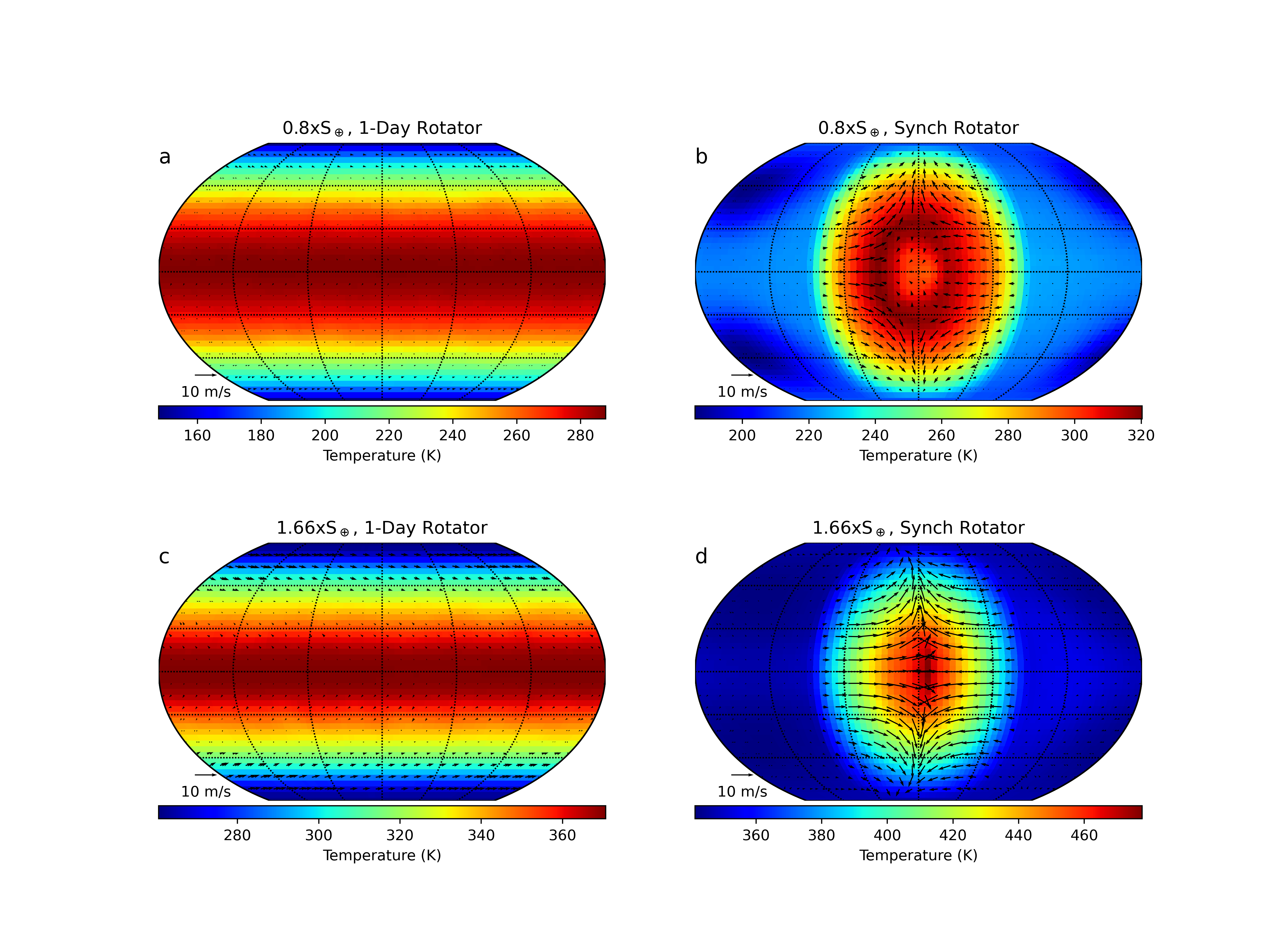
Figure 1: Maps of ground air temperature and wind speed for the representative 0.8 S_⊕ 1-day (a) and synchronous (b) rotators, and 1.66 S_⊕ 1-day (c) and synchronous (d) rotators. The temperature maps roughly follow expectations, with the synchronous rotators dominated by day- to night-side variation, and 1-day rotators dominated by latitudinal variation. Note that the color bars are different in each subfigure.

Once the simulations have converged, we used the Planetary Spectrum Generator (PSG, Villanueva et al., 2018, 2022) in order to obtain transmission spectra. PSG and the associated GlobES module uses the full three-dimensional output of the GCM to self-consistently perform the 3D radiative transfer calculations of the spectrum in transmission. Because ROCKE-3D only generates atmospheres up to pressures of 0.1 mbar and lower pressures can still impact transmission spectroscopy, we extended the atmospheres up to $\sim$10 nbar, assuming an isothermal profile and the same molecular mixing ratios, mimicking the procedure in Fauchez et al. (2022) (and similarly finding minimal differences). We also applied an additional pre-processor option to obtain the cloud mixing ratio and particle size variables for the liquid and water ice clouds. We followed the recommendations in the PSG handbook (Villanueva et al., 2022) for generating transmission spectra from the .aij* ROCKE3-D output files to ensure that the correct geometry was captured in our spectra.

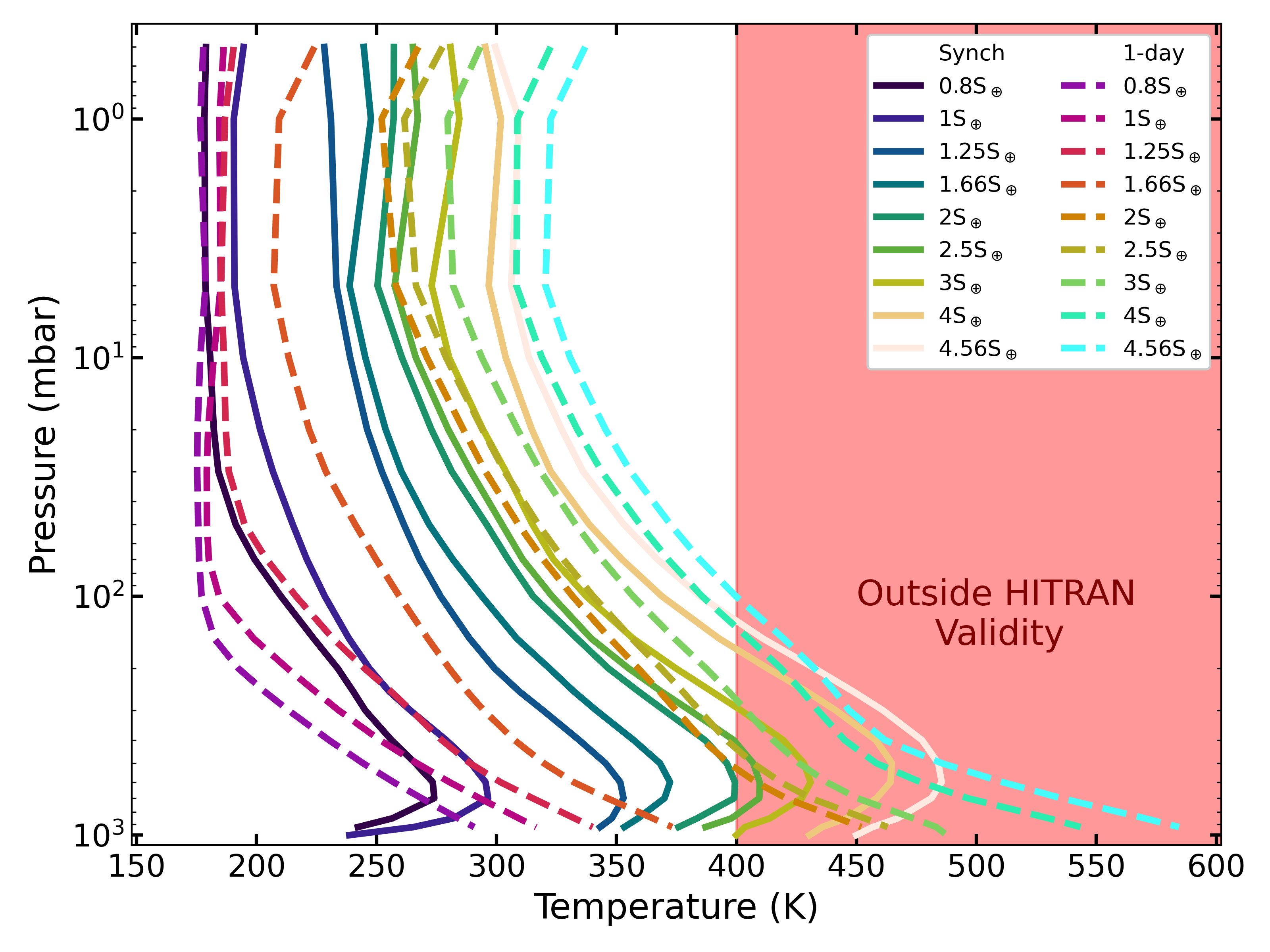
Figure 2: The pressure-temperature profiles of each simulation at the sub-stellar point (or longitude=0 for the 1-day rotators). The region where the HITRAN line list is inadequate is highlighted in red.

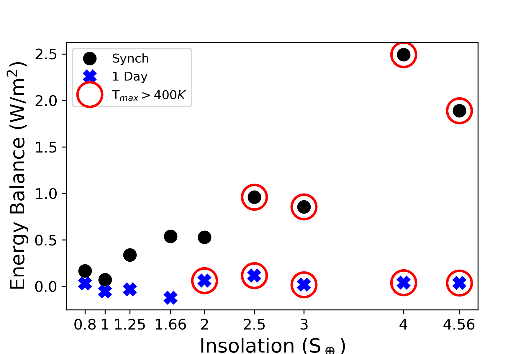
Figure 3: Here we show the energy balance of each simulation ordered by instellation. A value of 0 would indicate a perfectly equilibrated simulation. The one-day rotators are almost fully converged. The hottest synchronous rotators display non-zero net fluxes. But, values lower than $\sim$0.75 W m^-2 are sufficient to be considered converged (although see Section 2.2 next).

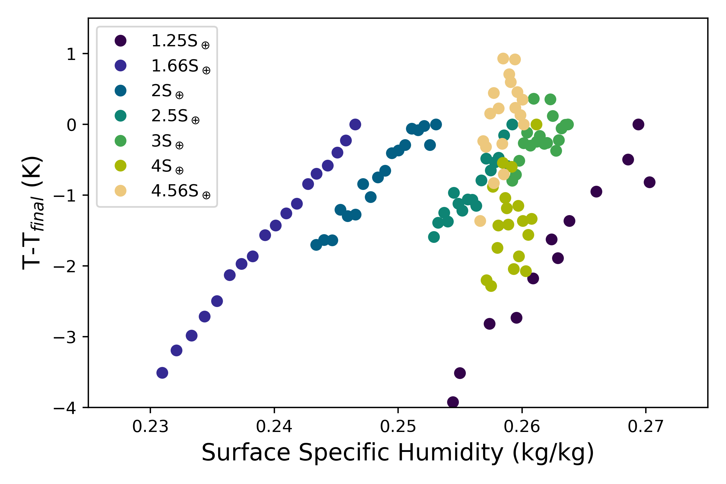
Figure 4: The median surface temperature of each simulation normalized by final temperature vs. the surface specific humidity. For most simulations, these values track each other closely, but this breaks down in the hottest (4 and 4.56 S_⊕) cases.

2.2 The Limits of ROCKE-3D

ROCKE-3D was originally developed as a branch of, and in parallel with, Earth climate simulation capabilities (ModelE2, Schmidt et al., 2014). As a result, it is best suited for modelling small, temperate planets. The parameters of the planet we chose to model are at the limits (and in some cases beyond the limits) of where ROCKE-3D and its underlying correlated-k tables are appropriate given our model setup. We therefore provide here a list of limitations of our model. Only recently has a different publicly available GCM tool that can bypass some of these limitations (particularly those related to the runaway greenhouse effect) been developed (Chaverot et al., 2023; Turbet et al., 2023).

1. Small exoplanets are thought to have a variety of bulk compositions, leading to great diversity in their atmospheres (see, e.g., Wordsworth & Kreidberg, 2022). However, to maintain relative simplicity, our realization of this planet is narrow. Our model is a dry, “desert” world (i.e., no oceans). It is decidedly not a water world (which this planet may be, per Luque & Pallé, 2022). Its atmospheric composition is entirely N₂/CO₂ with trace H₂O. It also does not include significant topography.

2. Our compositional choices result in an atmosphere that likely does not have significant haze particles, photochemical or otherwise. Such hazes are thought to be common in warm exoplanet atmospheres (e.g., Gao et al., 2021). However, cool planets with temperatures similar to Earth appear to have efficient haze removal (Yu et al., 2021), so for our cooler instances, this is a motivated decision. At the same time, different atmospheric compositions (e.g. added methane to serve as a haze precursor) could result in observationally and climatogically significant hazes (Cohen et al., 2024).

3. Some of our hotter simulations, in parts of their atmosphere, exceed the limits at which the HITRAN molecular line list for H₂O is valid (see Figure 2), which results in problems for the radiative transfer code (Goldblatt et al., 2013). We include them here for completeness. Given our model setup, the physics of these hotter simulations are qualitatively sensible, since in both rotation regimes, they converge on a perpetually sub-saturated atmosphere as the temperature increases. These models produce spectra that resemble the higher-temperature simulations that are within the valid HITRAN temperature range. However, we cannot be confident in results outside the valid HITRAN range; thus, the bulk of our conclusions are drawn from the cooler planets, where no line-list issues exist.

4. We self-consistently calculate the orbital distance and rotation rate for each instance, meaning that the synchronous rotators approach the dynamical regime sampled by the 1-day rotators in rotation period as we move to higher instellation (at a 1 day orbital period they would have the same rotation period). Our hottest simulation has an orbital period of $\sim$7 days, which likely crosses into the Rhines rotation regime (Haqq-Misra et al., 2018). However, per the previous point, there is limited information to be gained from the hotter simulations, and the cooler cases resemble the slow rotators (Figure 1).

5. Our simulations are largely within the net flux threshold for convergence ($\lesssim$1 W m^-2 deviation from 0), and for the most part their temperatures do not fluctuate significantly in the final stages of the model, which is a useful stability indicator (Figure 5). However, particularly in the hottest synchronous cases, there is non-zero net flux (see Figure 3) and persistent temperature fluctuation at the 1-2 K level. Even though the hottest cases still broadly appear converged, there are clear limitations on what information can be extracted from them, and we include them here primarily for completeness.

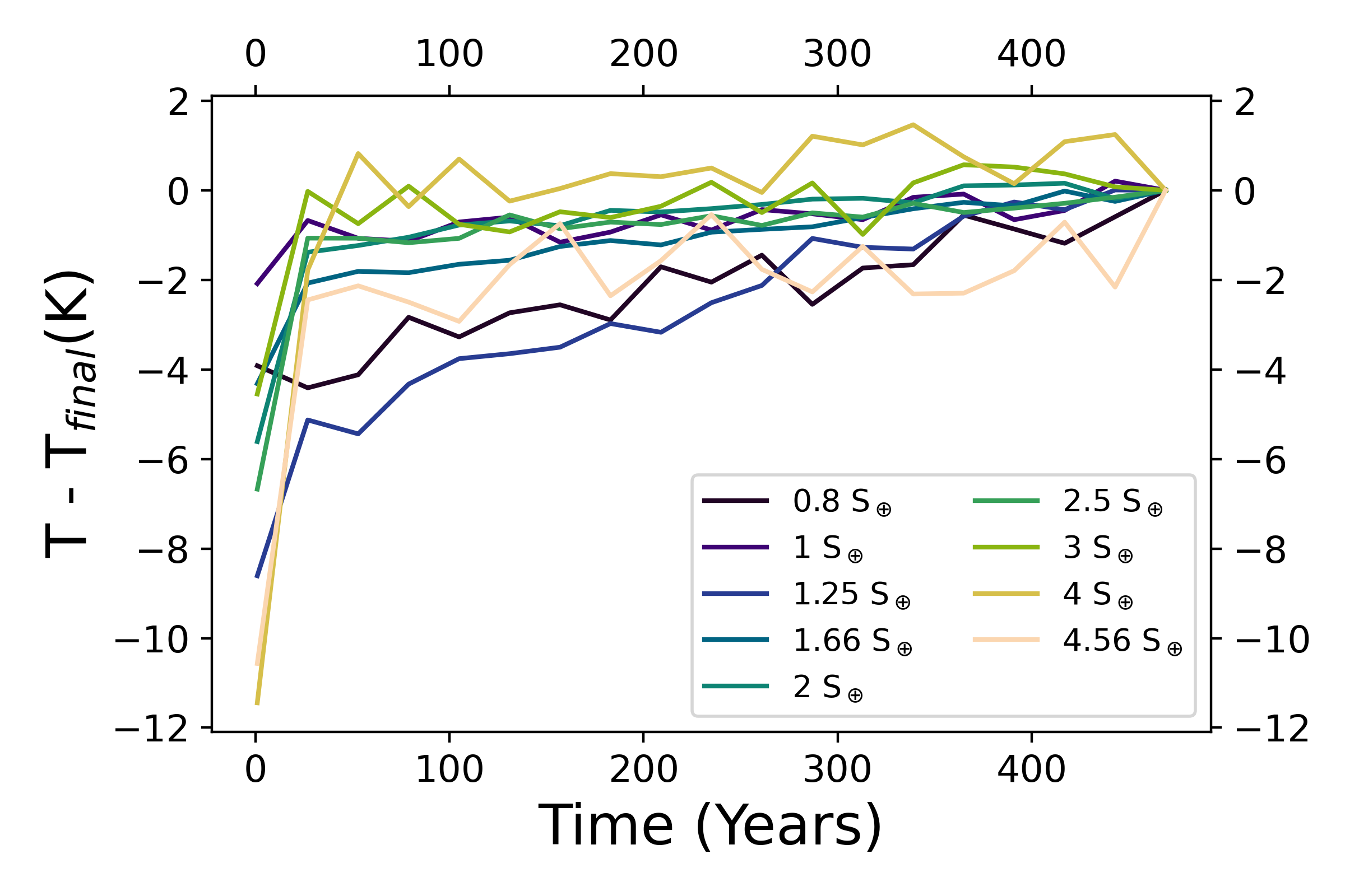
Figure 5: The average surface temperature at each time point of our synchronously rotating models, shown for each irradiation step. The hottest of these models, particularly the 4 and 4.56 S_⊕ cases, still have temperature fluctuations at the $\sim$few K level.

3 Some Synchronous and 1-Day Rotators Have Different Spectra

The primary result of our work can be summarized as follows: for planets from roughly temperate-to-Venus levels of irradiation (1-2 S_⊕), the near-infrared transmission spectra of planets in the two rotation regimes we consider are visibly distinct. This is clear in Figure 6, where we show the synchronous vs 1-day rotator transmission spectra for each model in our instellation grid. Note that this representation differs slightly from the usual representation of transmission spectra. Rather than showing total depth (i.e., including the entire planetary radius), or showing only feature height above the opaque planet + continuum (i.e., minimum of feature height in all plots is 0), we show feature amplitude above the planet surface only. Thus the opaque atmosphere also contributes to the continuum, resulting in “depths” that have minima $\gtrsim$3ppm. We have selected the 0.5-5 micron wavelength region specifically because this is where JWST will be able to obtain precise spectra for small planets.

In the simulations up to roughly Venus irradiation, the spectra are distinct in terms of their spectral continuum and features, amplitude of features, and scattering slope, given a spectrum of arbitrarily high precision (see Section 4.2 for a discussion of the implications of these differences for real observations). In the following subsections, we will discuss the characteristics of these differences and the factors that drive them in more detail. We discuss clouds first and then climate factors. We note that these factors are of course intrinsically linked, but are frequently measured separately in atmospheric retrievals, where a deck of grey clouds at arbitrary altitude is a common tool used to match observations (e.g., Welbanks & Madhusudhan, 2021).

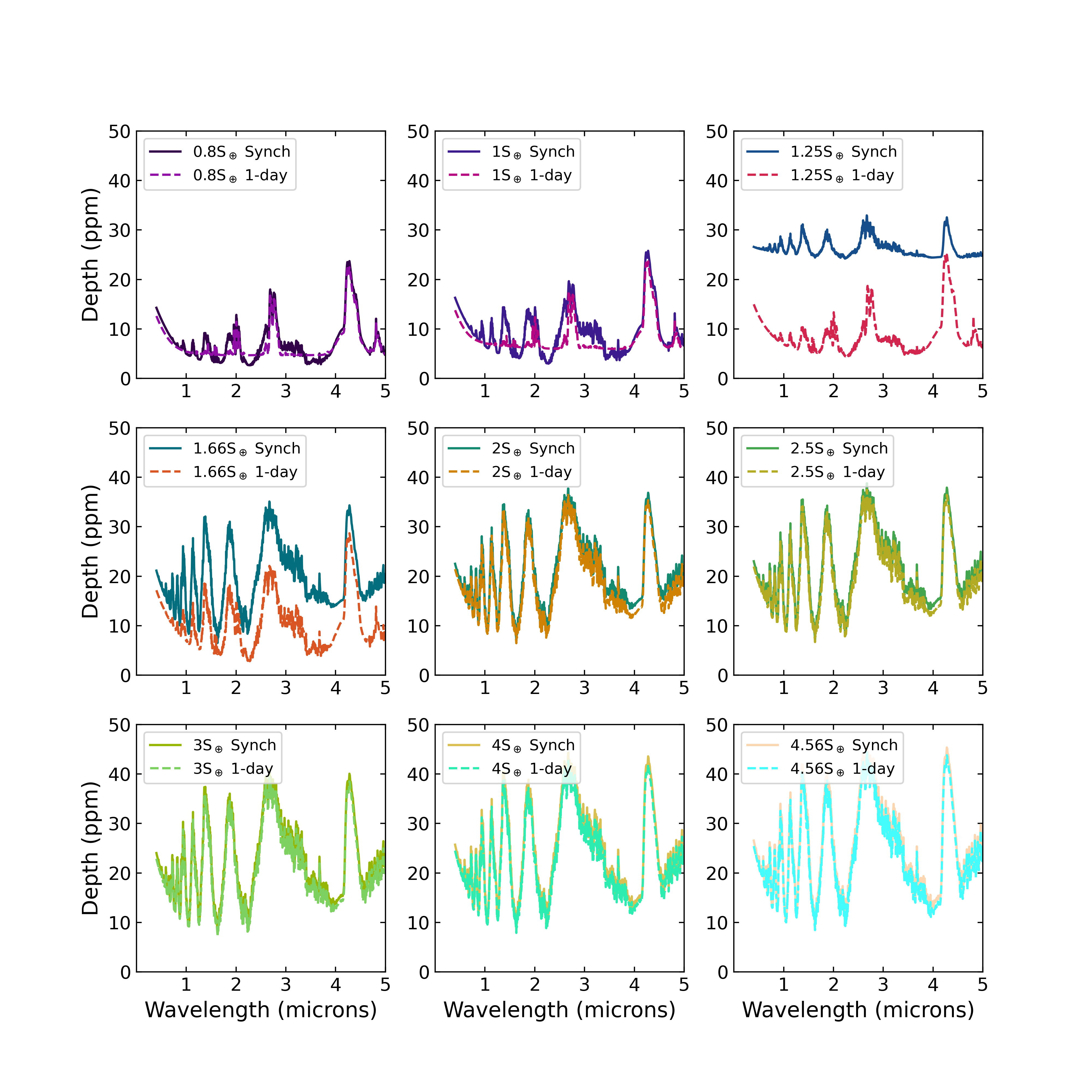
Figure 6: The spectrum of each simulation in our explored parameter space. Each has the same composition (N₂-dominated, trace CO₂ and H₂O; Table 1). Each box shows the synchronous and 1-day rotator cases for different instellation values, which are printed in the legend. Up to 1.66 S_⊕, the transit spectra are distinguishable. In warmer cases, the differences disappear.

3.1 Differences I: Clouds

ROCKE-3D, and therefore our simulations, considers water (liquid and ice) clouds only. The full treatment of clouds in ROCKE-3D is described in Way et al. (2017), Section 4.2. To briefly summarize, the simulation treats the dynamics, thermodynamics, and microphysics of convection for a mass flux of rising moist air (Del Genio et al., 2015). The simulation maintains sub-saturated grid conditions (in contrast to some other GCMs) in cells where updrafts originate. The sub-gridbox treatment allows nonzero cloud fractions to appear without full saturation of a grid cell and are instead determined from local humidity and stability (see del Genio et al., 1996; Schmidt et al., 2006, 2014). We refer the reader to Way et al. (2017) for the full model details.

Clouds are a well-known and significant driver of the shapes of exoplanet spectra (e.g., Fauchez et al., 2019; Komacek et al., 2020; Suissa et al., 2020; Gao et al., 2021). Our simulations are no different: many spectral differences that we show here are clearly driven by clouds. This is evident by inspection, particularly in the coolest cases where a flat (i.e., spectrally grey) continuum opacity characteristic of clouds is present (top row, Figure 6).

These continuum differences become less pronounced and eventually disappear in both rotation cases once we raise the instellation as high as 2 S_⊕. This occurs because the hotter simulations have little to no cloud cover, and in a cloudy atmosphere, the continuum level is defined by the altitude of the optically thick cloud deck. In Figure 7, we show the total cloud cover in each column of grid cells as a function of longitude to highlight the terminator region, which determines the transmission spectrum. For the synchronous rotators, once instellation rises to 1.66 S_⊕ case, cloud cover becomes very low, and in the hotter cases still, there is negligible cloud cover. In all cases, the cloud cover is almost exclusively stratiform. Convective cloud cover is negligible except in the coolest case (0.8 S_⊕), where it makes up a few % of the total cloud coverage.

Broadly, this result is in agreement with Kopparapu et al. (2016), who find as they increase the instellation of their synchronous rotators, this drives the water vapor greenhouse, increasing absorption at high altitudes. This in turn decreases the lapse rate and suppresses convection, muting cloudiness. The 1-day rotators still retain appreciable cloud cover in the 1.66 S_⊕ case, being cooler than the synchronous rotators at the same irradiation (Figure 2), but follow the same trend of moving to lower and eventually no cloud cover as instellation increases.

To understand why this is the case, we show the specific humidity profiles: by the time the instellation reaches 2 S_⊕, both rotation regimes have converged on a perpetually sub-saturated atmosphere. The transition occurs at different irradiation thresholds for the synchronous and 1-day cases because of their different climates - the synchronously rotating cases are hotter than the 1-day rotators in the intermediate instellation cases (Figure 2). Note in the 1.66 S_⊕ case (Figure 6, middle left panel), the synchronous rotator’s spectrum has already begun to look identical to the hottest cases, but not so for the 1-day rotator.

Why do the highest-instellation cases have roughly identical spectra (modulo a small offset), regardless of rotation rate? First, we caution the reader that in these cases (certainly by 2.5 S_⊕), we have begun to enter a regime of questionable validity of the HITRAN line lists (Figure 2; Goldblatt et al., 2013), so these results should be treated with caution. However, the behavior can still be interpreted qualitatively. The only spectrally active characteristics of our model atmospheres are CO₂, H₂O, N₂-N₂ collision-induced absorption (CIA), and clouds. Without clouds and their potential associated climate feedback, the hottest cases are composed of perpetually sub-saturated water, N₂, and trace CO₂, whose medium resolution spectral signatures are not changing significantly with temperature. The amplitude of spectral features does increase slightly with instellation, as expected given the temperature dependence of the atmospheric scale height.

Remaining for discussion is the 1.25 S_⊕ case, in which the synchronous rotator displays apparently anomalous behavior. The transit depth above the defined surface (i.e., the continuum height) is consistently $\sim$25 ppm, whereas the other simulations range from 2-10 ppm from coolest to warmest. The reason for this appears to be significantly higher-altitude clouds than in any other simulations, which we show in Figure 8. The 1.25 S_⊕ case synchronous rotator has terminator clouds more than an order of magnitude higher in the atmosphere than either its cooler sychronous rotator counterparts or its 1-day rotator analog, resulting in this “lifted” continuum. Although the 1.66 S_⊕ case has even higher altitude clouds, their coverage is extremely low (Figure 7), so they do not contribute significantly to the opacity. This can also be seen comparing the corresponding panels in Figures 6 and 9, where eliminating the clouds minimally changes the difference between rotators.

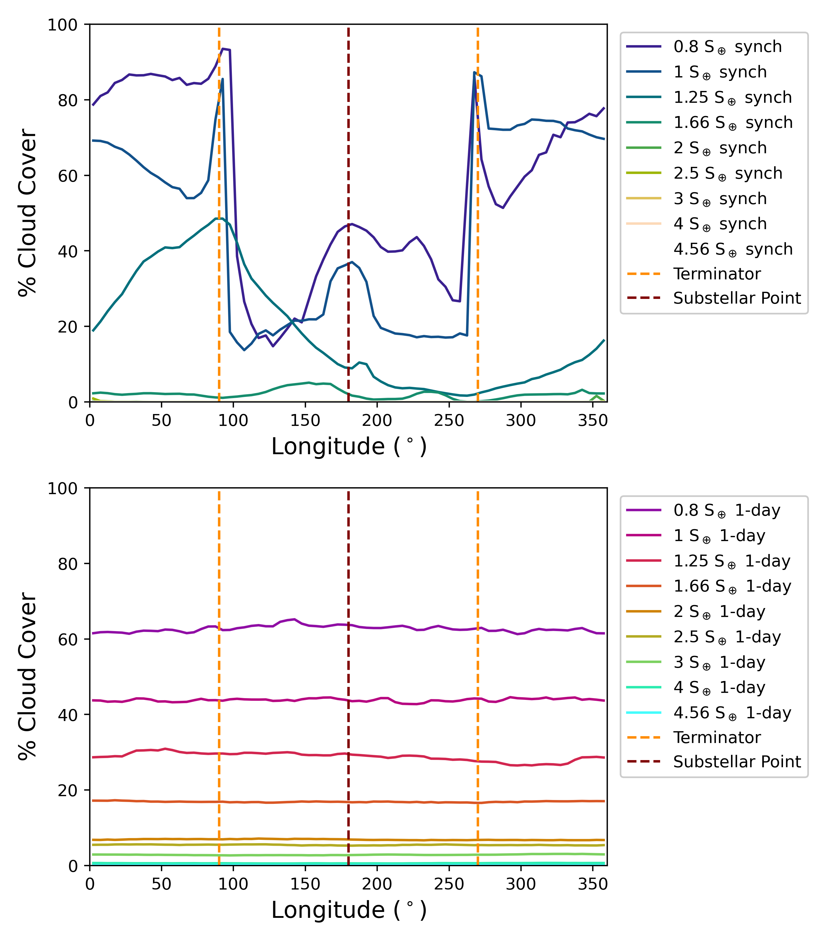
Figure 7: The mean percentage cloud cover of each grid cell plotted by longitude, marginalizing over latitude, for the synchronous rotators (top) and 1-day rotators (bottom). Cloud cover drops precipitously above $\sim$1.25 S$\oplus$ for the synchronous rotators, but persists to higher instellation for the 1-day rotators.

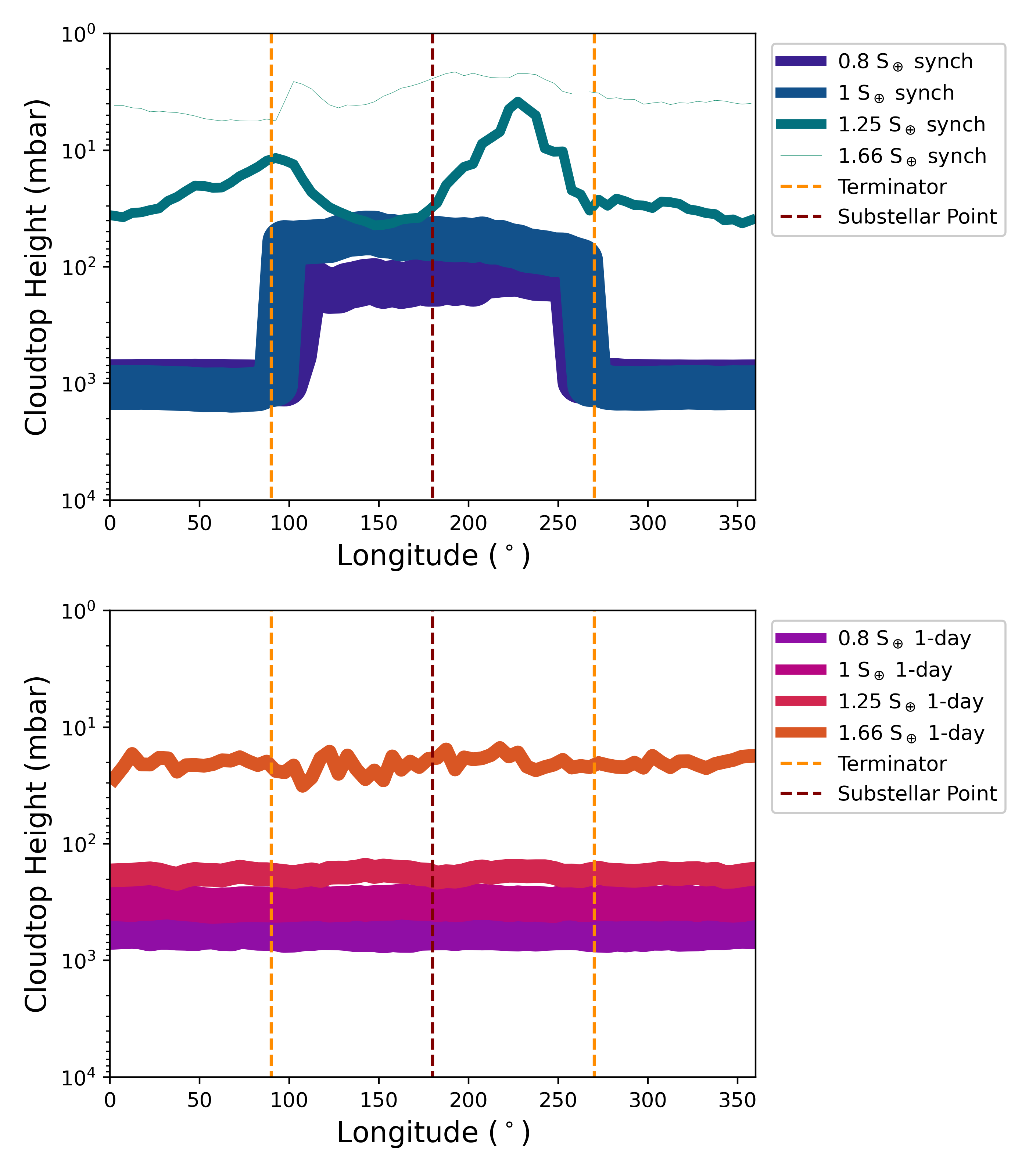
Figure 8: The median cloudtop height in each grid cell, marginalized by longitude, for the synchronous (top) and 1-day (bottom) rotators. The line widths correspond to the cloudtop height shown in Figure 7. In the 1.25 S$\oplus$ synchronous rotator case, the cloud is almost an order of magnitude higher at the terminator than for the 1-day case. Note that cases hotter than 1.66 S$\oplus$ are not shown because they contain no longitude columns of entirely non-zero cloud cover.

3.2 Differences II: P-T Profiles and Humidity

Clouds are a significant driver of the differences in our spectra, but not the only one. In order to test this, we repeated our procedure for generating the spectra with globes and PSG, but with clouds disabled. The results can be seen in Figure 9, where differences persist in some of our spectra despite the absence of clouds when calculating the transmission spectrum. We emphasize that in this case, we are only “turning off” clouds in the spectrum calculation, but the resulting spectrum is created from a simulation whose climatology was sculpted by clouds. This exercise is only a diagnostic of what transmission spectrum feature differences are directly caused by clouds. Qualitatively, the continuum absorption is more similar between rotators in the cloud-free cases (as expected), but some feature heights remain different. In particular, the 1.25 and 1.66 S$\oplus$ cases show significant differences in the amplitude of the water features from 1-3 $\mu$m, even in the spectral absence of clouds. As before, in the warmest cases the spectra are indistinguishable.

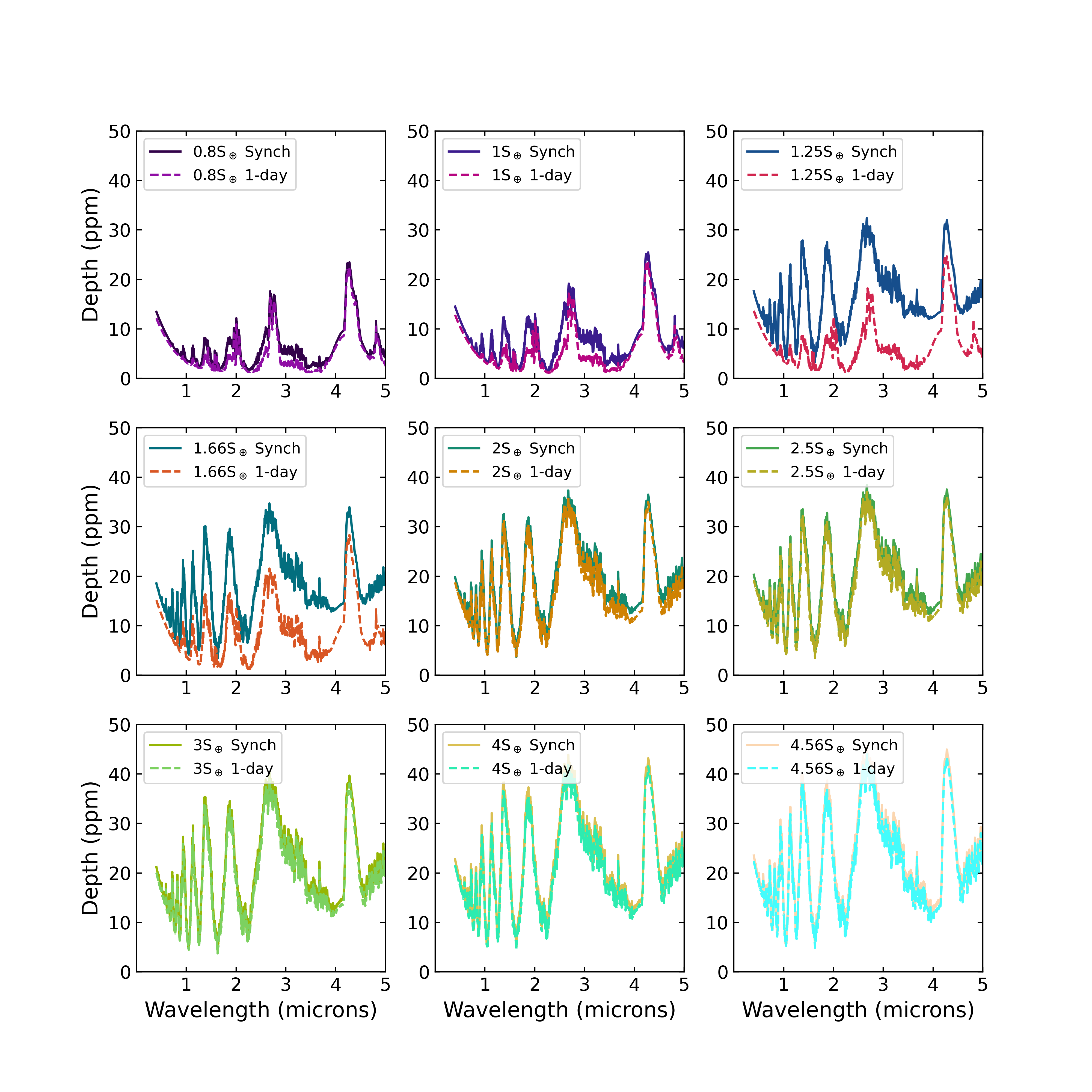
Figure 9: The spectra of each instantiation of our simulation with the optical and spectral effects of clouds removed. As in Figure 6, each box shows the synchronous and 1-day rotator cases for different instellation values, which are printed in the legend. Despite the absence of clouds, visible (though smaller) differences persist in the spectra of less-irradiated models.

What is driving these persistent differences? Given the relative simplicity of our models, the atmospheric pressure-temperature and humidity profiles are the two prime suspects. The atmospheric $\tau=1$ surface will change as the water abundance varies in the atmosphere, represented by these two factors. The 1.25 S_⊕ case, along with the 1.66 S_⊕ case, have the most qualitatively significant differences between the two rotators’ cloud-free spectra. Revisiting the pressure-temperature profiles in Figure 2, we can see that the temperature difference between synchronous and 1-day rotators is largest in these two cases. This will of course drive some differences in the scale height. However, more significantly, these temperature differences are driving the synchronous rotators in these two cases to reach a just sub-saturated state, while the atmospheres of the 1-day rotators are drier (Figure 10). This is likely the dominant driver of spectral differences in the cloud-free cases.

Driven by the pressure-temperature profile, the water content of the atmosphere also differs significantly between these cases (Figure 10). In the 1.25 S_⊕ case, the hotter synchronous rotator has already moved much of its surface water into atmospheric humidity, where the 1-day rotator remains fairly dry across all latitudes. Tracing the specific humidity across instellation for each rotation case, there is a clear transition from relatively dry to sub-saturated atmospheres. However, the break point occurs earlier (i.e, at lower instellation) for the synchronous rotators than the 1-day. The higher global temperatures (at least in intermediate cases) of the synchronous rotators are the likely driver of this.

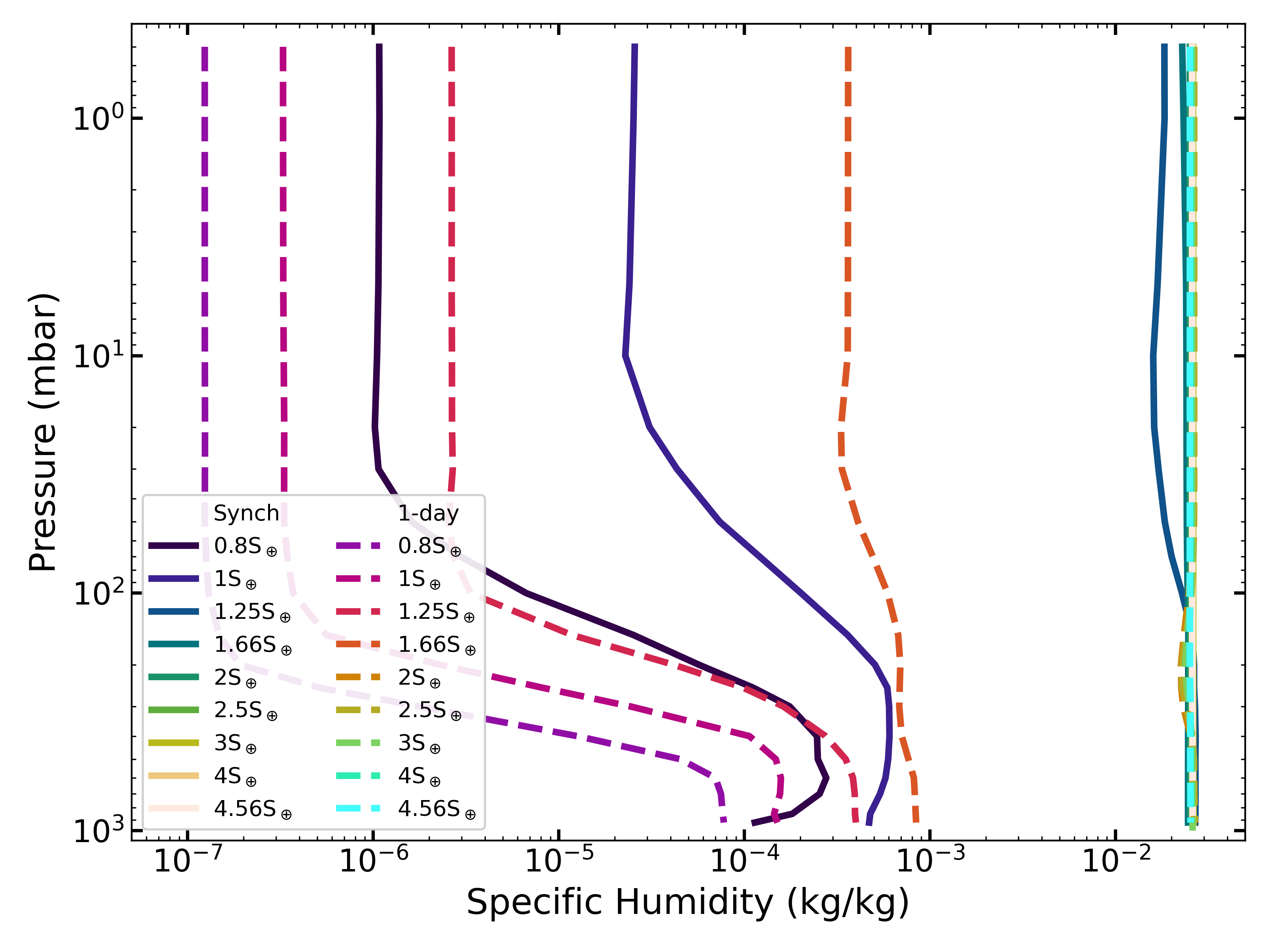
Figure 10: The mean pressure-humidity profile for the 0.8 through 2 S_⊕ cases. The transition to nearly sub-saturated atmospheres occurs at lower irradiation for the synchronous rotators than the 1-day rotators.

4 Discussion

4.1 Comparison To Previous Work

Before discussing the observational characteristics of our simulations, we continue the thread of Sections 3.1 and 3.2 and compare the climatology of our simulations to previous works which investigated similar scenarios. Much work on super-Earths has focused on water worlds (e.g., Yang et al., 2013; Sergeev et al., 2022). We selected the Hab 1 case (Sergeev et al., 2022) from the TRAPPIST-1 Habitable Atmosphere Intercomparison (THAI) series of papers (Turbet et al., 2022; Sergeev et al., 2022; Fauchez et al., 2022) as a “standard” water world suitable for comparison to our simulations. Both have an N₂-dominated atmosphere with 400ppm CO₂, although our simulations are much drier: the ROCKE-3D implementation of Hab 1 has a 90-meter global ocean, compared to our simulations whose only water is in the moist soil. Hab 1 is also slightly less irradiated than our coolest simulation (900 W m^-2 vs 1089 W m^-2 in our 0.8  S_⊕ case).

Our simulations’ behavior differs from that of the THAI Hab 1 case, which has substantial cloud cover at the substellar point frequently seen in synchronous rotators in 3-D (e.g., Yang et al., 2013, 2014; Kopparapu et al., 2016). Instead, our simulations qualitatively better resemble the water-limited cases explored in Lobo et al. (2023), with less dayside cloud cover and correspondingly lower dayside albedo. We find similarly large ($\gtrsim$100 K) day-to-night temperature variations to the water-limited models in Lobo et al. (2023), which they attribute to less energy transport in a drier atmosphere compared to their aquaplanet cases. Our findings of more nightside cloud cover (in the less-irradiated cases; Figure 7) also match the findings in Turbet et al. (2023), who investigated what was required for a “hot start” case to condense liquid water oceans, analogous to the likely formation conditions of rocky planets. The mechanism that drives the nightside cloud is different between their study and ours. In their case, the high-altitude water vapor is an efficient absorber of incoming stellar radiation, and the resulting heating of the upper atmosphere breaks dayside convection, preventing the formation of convective clouds. Our cooler simulations have no such high-altitude water content (Figure 10), and instead convection is likely inhibited by lack of available atmospheric water.

We also investigate potential variability in our simulations, significant in light of the findings of Fauchez et al. (2022) that inter-transit variability was larger than spectral differences between, for example, O₂ and H₂O (Wunderlich et al., 2020). Outputting the simulation instances used to generate Figures 6 at one-month intervals for two years, we measure the variation in transit depth of the 1.8$\mu$m bandpass, since it and other continuum regions are the most highly varying part of transmission spectra in the near-infrared (Fauchez et al., 2022). We find that the standard deviation of the spectra in this region is at most around 5 ppm (Figure 11). This is roughly consistent with the amplitudes found in previous variability studies (e.g., May et al., 2021; Song & Yang, 2021; Cohen et al., 2022). The variability peaks for the synchronously rotating simulations in the 1.25 S_⊕ and 1.66 S_⊕ cases, which we observe to have tenuous, high-altitude clouds that are prone to fluctuation. Meanwhile, for the 1-day rotators, the variability increases with irradiation until the hottest case. This may be because the 1-day rotators maintain nonzero cloud cover until the hottest instance (Figure 7), although we reiterate the cautions of Section 2.2 around the results of these hottest instances. In any case, this peak variability amplitude of $\sim$5 and $<$1 ppm from the synchronous and 1-day rotators, respectively, in the 1.25 S_⊕ case is not sufficient to wash out the maximum $\sim$20 ppm difference between their spectra, although the difference will be obscured.

Figure 11: The standard deviation of the transit depth in the 1.8 $\mu$m bandpass for monthly cadence simulations over two years. Probably because of their differing cloud behavior, the synchronous and 1-day rotators have differing patterns of variability.

A final point is that the variability itself could be useful as an indirect diagnostic for rotation rate. The scale of this effect is not relevant to JWST observations (for which single transit observations have maximum characteristic precision of around 20ppm), but may be of interest to next generation facilities like the Habitable Worlds Observatory, especially in intermediate-instellation cases where the variability signal differs considerably between rotation regimes. We do reiterate, however, that the exact variability conditions will depend on model choice and setup (Sergeev et al., 2022; Fauchez et al., 2022), so additional testing would be required to confirm this result. This is particularly important given the water-limited nature of our simulations, which as discussed yields important differences when compared to “aquaplanet” simulations. Overall, this work suggests that the transmission spectra of water-limited super-Earths will be fairly robust to inter-transit atmospheric variability, although the variability will make the detection of small effects like those we examine here more difficult.

4.2 The Differences We Present Are Difficult to Individually Observe

We have shown above that there are visible differences in the idealized transmission spectrum of a small planet depending on whether it rotates synchronously or not. However, with real observations of an atmosphere identical to the one we model, it would be difficult or impossible to extract these differences. Observations of small planets are already challenging. In this case, we find at best a model difference of roughly 20 ppm, a precision that could only be achieved with large numbers of JWST transits (e.g., Pidhorodetska et al., 2021). Furthermore, the difference would require observations beyond 5 $\mu$m to break the degeneracy with a larger planetary radius (Figure 6), but even JWST’s Mid-Infrared Instrument is probably unsuitable for transmission spectroscopy (though not emission, which we do not simulate here; e.g., Greene et al., 2023; Zieba et al., 2023) observations of small planets (Batalha et al., 2018). In any case, this difficulty was to be expected given our model setup: we are considering mostly N₂/CO₂ atmospheres (i.e., high mean molecular weight). This is a fairly “pessimistic” (from the observational perspective) case even for a super-Earth atmosphere (e.g., Pidhorodetska et al., 2021).

Even in a more “optimistic” (i.e., lower mean molecular weight) atmosphere, this work is not sufficient to claim that planetary rotation rate can be identified from spectra alone. The most significant differences that we present here are driven by clouds, but cloud formation physics is not fully understood (e.g., Gao et al., 2021) and is parameterized within our model. Different and potentially more detailed parameterizations may yield different results (e.g., Sergeev et al., 2020; Lefèvre et al., 2022). Thus, a “rotation rate signature” will inevitably be degenerate with other physical processes that drive cloud formation and climate such as initial water inventory. As mentioned above, our simulations do not explore the formation of hazes, which are likely a significant opacity source in planetary atmospheres (e.g., Gao et al., 2021). That said, this work provides a first pass look at how future observatories, in combination with bespoke forward models, may be able to observationally investigate planetary rotation rate.

We must also note that ROCKE-3D is not the only GCM, and there is known to be dispersion in the results that different GCMs produce, depending on the details of their methodology. In particular, the THAI collaboration performed intercomparisons between ROCKE-3D, the Exoplanet Community Atmospheric Model (ExoCAM), The Laboratoire de Météorologie Dynamique—Generic model (LMD-G), and the Met Office Unified Model (UM). Sergeev et al. (2022) treat the moist cases among the THAI models, of which our model is most similar to their Hab 1 state. As described above, Hab 1 has significantly more water than our model (ROCKE-3D’s implementation of Hab 1 features a 90 m global ocean) and less irradiated than most of the models we consider, but is otherwise similar (1 bar N₂ atmosphere with $\sim$400ppm CO₂). They find that the GCMs have broadly similar cloud behavior (i.e., large cloud decks at the substellar point, following, e.g., Yang et al., 2013, 2014; Kopparapu et al., 2016), but with important differences between them. ROCKE-3D produces atmospheres with the largest fractional cloud cover, while ExoCAM produces clouds with both the highest altitude and highest mixing ratio. Clouds are the main (though not only; Figure 9) driver of spectral differences between our models, so a GCM like LMD-G (the least cloudy of the four studied by Sergeev et al., 2022) may find smaller differences between rotation states. Considering the transmission spectra resulting from the various GCMs’ Hab 1 models, Fauchez et al. (2022) find up to a 50% spread in the number of observations required to confidently detect CO₂, which functions as a proxy for the ability to detect the presence of an atmosphere given the relative magnitude of the 4.3 $\mu$m CO₂ feature. Given the nonlinear cloud behavior we find in our simulations, the “GCM uncertainty factor” is relevant to our predictions as well, and similar studies with other GCMs would be needed to validate our predictions.

4.3 Lessons for Wider Parameter Spaces

Because of the evident non-linearity of 3D simulations (see e.g. the formation of a high-altitude cloud deck in the 1.25 S_⊕ synchronous rotator case), we cannot straightforwardly “scale up” our simulations to make predictions for planets in other parts of parameter space, like larger sub-Neptunes, H₂O-rich “water worlds,” or hotter terrestrials that will form the majority of those observed with JWST. However, some of the physical processes we identify here are likely relevant to those planets.

First, we describe some non-linearity in cloud formation and behavior across our simulations. Although the average percentage cloud cover follows a fairly straightforward pattern from significant clouds at the coolest temperatures to little/no cloud cover in hotter cases (Figure 7), this does not fully capture the cloud behavior. The 1.25 S_⊕ synchronous rotator case exemplifies this best, with high altitude clouds (Figure 8) that affect the behavior of the spectrum (Figure 6, upper right panel) and climate (Figure 2). This result complicates ongoing efforts to understand trends in cloud/haze patterns in exoplanet atmospheres (e.g., Gao et al., 2021; Yu et al., 2021; Brande et al., 2024), and suggests any such relationships will likely have an inherent, effectively stochastic level of scatter due to nonlinear effects like these. Despite the model limitations we describe in Section 2.2, there is no reason to think that effects of this sort are unique to our parameter space. This further suggests that 1D forward models may be insufficient for predicting an individual planet’s cloud behavior.

A related implication for our population-level understanding of exoplanet cloud behavior is what our results suggest of the behavior of condensibles other than water. While more work would be needed to determine how commonly the transition from condensible to too-rarefied occurs for a given species, the result that condensation produces nonlinear and inhomogeneous effects should be broadly applicable. Various species are thought to play the role of condensibles on hot exoplanets that they do not in our solar system, such as KCl and MgSiO₃, among others (e.g., Gao & Benneke, 2018; Herbort et al., 2022). Although the physics and dynamics of atmospheres where these species are the dominant condensibles will be different from the simulations we present here, similar effects could play out, with limited transfer from a lower-atmosphere reservoir broadly analogous to a limited starting water inventory. Our ultimate point is that this further motivates 3D modelling for individual planets to better understand their cloud and climate behavior.

4.4 Rotation Rate Can Inform Sample Selection

In addition to the implications for next-generation observations of individual small planets, where rotation rate could be a parameter inferred by spectroscopic observations, our work here has implications for current observational campaigns. In particular, efforts to infer the presence of a small planet atmosphere from JWST transmission spectroscopy requires finding signals very close to the limit of what it is possible to detect. In constructing a sample of moderately irradiated planets for observation, and subsequently attempting population-level inferences, estimated rotation rate will play a role. Although there is no mechanism currently to determine rotation rate directly, system characteristics that impact rotation rate, especially planetary multiplicity (Vinson et al., 2019; Chen et al., 2023; Shakespeare & Steffen, 2023), will need to be considered.

5 Conclusions

The key takeaways of our work are as follows:

1. We created a suite of simulations of a fairly dry super-Earth exoplanet with a N₂/CO₂ atmosphere and demonstrated that, at Earth-like levels irradiation (up to $\sim 1.66$S_⊕), changing the planetary rotation rate has a corresponding effect on the transmission spectrum. These differences are not observed in hotter planets.

2. We show that the differences in transmission spectra are driven primarily by the presence of non-convective cloud decks on the terminator. The atmospheric water column profiles also drive some spectral differences at lower temperatures, before the atmosphere becomes perpetually sub-saturated.

3. Even though our particular simulations, which have high mean-molecular-weight nitrogen atmospheres, do not show differences at levels that could be detected with reasonable expenditures of JWST time, planets that are larger, have less dense atmospheres, or have even smaller host stars could be laboratories for this phenomenon. However, we reiterate that the differences between transmission spectra of synchronous vs. 1-day rotators should be investigated with multiple GCMs to be considered robust, given previously shown dispersion in outcomes from different models. As well, publicly available GCMs capable of handling larger, hotter planets will be important for confirming the applicability of our results outside of the specific parameter space that we explore.

6 Acknowledgements

The authors wish to thank Geronimo Villanueva and Eric Wolf for discussions and technical feedback that greatly aided the completion and quality of this manuscript. N.S. wishes to thank Natalie Batalha for mentorship that also greatly enhanced the quality of this manuscript. Support for N.S. was provided by NASA through a grant from the Space Telescope Science Institute, which is operated by the Association of Universities for Research in Astronomy, Inc., under NASA contract NAS 5-03127. N.S. gratefully acknowledges support from the Heising-Simons Foundation through grant 2021-3197. This material is based upon work supported by NASA’S Interdisciplinary Consortia for Astrobiology Research (NNH19ZDA001N-ICAR) under award number 19-ICAR19_2-0041. This work was supported by NASA’s Nexus for Exoplanet System Science (NExSS) and the NASA Interdisciplinary Consortia for Astrobiology Research (ICAR). Resources supporting this work were provided by the NASA High-End Computing (HEC) Program through the NASA Center for Climate Simulation (NCCS) at Goddard Space Flight Center. C.E.H. acknowledges support through the ROCKE-3D ICAR grant.

References

- Angelo et al. (2017) Angelo, I., Rowe, J. F., Howell, S. B., et al. 2017, The Astronomical Journal, 153, 162
- Batalha et al. (2018) Batalha, N. E., Lewis, N. K., Line, M. R., Valenti, J., & Stevenson, K. 2018, ApJ, 856, L34, doi: 10.3847/2041-8213/aab896
- Benneke & Seager (2012) Benneke, B., & Seager, S. 2012, The Astrophysical Journal, 753, 100, doi: 10.1088/0004-637X/753/2/100
- Bony et al. (2015) Bony, S., Stevens, B., Frierson, D. M. W., et al. 2015, Nature Geoscience, 8, 261, doi: 10.1038/ngeo2398
- Brande et al. (2024) Brande, J., Crossfield, I. J. M., Kreidberg, L., et al. 2024, ApJ, 961, L23, doi: 10.3847/2041-8213/ad1b5c
- Carone et al. (2014) Carone, L., Keppens, R., & Decin, L. 2014, MNRAS, 445, 930, doi: 10.1093/mnras/stu1793
- Chaverot et al. (2023) Chaverot, G., Bolmont, E., & Turbet, M. 2023, arXiv e-prints, arXiv:2309.05449, doi: 10.48550/arXiv.2309.05449
- Checlair et al. (2017) Checlair, J., Menou, K., & Abbot, D. S. 2017, ApJ, 845, 132, doi: 10.3847/1538-4357/aa80e1
- Checlair et al. (2019) Checlair, J. H., Olson, S. L., Jansen, M. F., & Abbot, D. S. 2019, ApJ, 884, L46, doi: 10.3847/2041-8213/ab487d
- Chen et al. (2023) Chen, H., Li, G., Paradise, A., & Kopparapu, R. K. 2023, ApJ, 946, L32, doi: 10.3847/2041-8213/acbd33
- Cloutier, R. et al. (2019) Cloutier, R., Astudillo-Defru, N., Bonfils, X., et al. 2019, A&A, 629, A111, doi: 10.1051/0004-6361/201935957
- Cohen et al. (2022) Cohen, M., Bollasina, M. A., Palmer, P. I., et al. 2022, ApJ, 930, 152, doi: 10.3847/1538-4357/ac625d
- Cohen et al. (2024) Cohen, M., Palmer, P. I., Paradise, A., Bollasina, M. A., & Tiranti, P. I. 2024, AJ, 167, 97, doi: 10.3847/1538-3881/ad1ab9
- Colose et al. (2021) Colose, C. M., Haqq-Misra, J., Wolf, E. T., et al. 2021, The Astrophysical Journal, 921, 25
- Cowan & Abbot (2014) Cowan, N. B., & Abbot, D. S. 2014, The Astrophysical Journal, 781, 27, doi: 10.1088/0004-637X/781/1/27
- Del Genio et al. (2019) Del Genio, A. D., Way, M. J., Kiang, N. Y., et al. 2019, ApJ, 887, 197, doi: 10.3847/1538-4357/ab57fd
- Del Genio et al. (2015) Del Genio, A. D., Wu, J., Wolf, A. B., et al. 2015, Journal of Climate, 28, 6419 , doi: https://doi.org/10.1175/JCLI-D-14-00832.1
- del Genio et al. (1996) del Genio, A. D., Yao, M.-S., Kovari, W., & Lo, K. K. W. 1996, Journal of Climate, 9, 270, doi: 10.1175/1520-0442(1996)009<0270:APCWPF>2.0.CO;2
- Del Genio et al. (2019) Del Genio, A. D., Kiang, N. Y., Way, M. J., et al. 2019, The Astrophysical Journal, 884, 75
- Demangeon et al. (2024) Demangeon, O. D. S., Cubillos, P. E., Singh, V., et al. 2024, A&A, 684, A27, doi: 10.1051/0004-6361/202348270
- Edson et al. (2011) Edson, A., Lee, S., Bannon, P., Kasting, J. F., & Pollard, D. 2011, Icarus, 212, 1, doi: 10.1016/j.icarus.2010.11.023
- Edwards (1996) Edwards, J. 1996, Journal of Atmospheric Sciences, 53, 1921
- Edwards & Slingo (1996) Edwards, J., & Slingo, A. 1996, Quarterly Journal of the Royal Meteorological Society, 122, 689
- Fauchez et al. (2019) Fauchez, T. J., Turbet, M., Villanueva, G. L., et al. 2019, ApJ, 887, 194, doi: 10.3847/1538-4357/ab5862
- Fauchez et al. (2022) Fauchez, T. J., Villanueva, G. L., Sergeev, D. E., et al. 2022, The Planetary Science Journal, 3, 213, doi: 10.3847/PSJ/ac6cf1
- Fujii et al. (2017) Fujii, Y., Del Genio, A. D., & Amundsen, D. S. 2017, The Astrophysical Journal, 848, 100
- Gao & Benneke (2018) Gao, P., & Benneke, B. 2018, ApJ, 863, 165, doi: 10.3847/1538-4357/aad461
- Gao et al. (2021) Gao, P., Wakeford, H. R., Moran, S. E., & Parmentier, V. 2021, Journal of Geophysical Research: Planets, 126, e2020JE006655, doi: https://doi.org/10.1029/2020JE006655
- Godfrey (1988) Godfrey, D. 1988, Icarus, 76, 335, doi: https://doi.org/10.1016/0019-1035(88)90075-9
- Goldblatt et al. (2013) Goldblatt, C., Robinson, T. D., Zahnle, K. J., & Crisp, D. 2013, Nature Geoscience, 6, 661, doi: 10.1038/ngeo1892
- Greene et al. (2023) Greene, T. P., Bell, T. J., Ducrot, E., et al. 2023, Nature, 618, 39, doi: 10.1038/s41586-023-05951-7
- Guzewich et al. (2021) Guzewich, S. D., Way, M. J., Aleinov, I., et al. 2021, Journal of Geophysical Research: Planets, 126, e2021JE006825
- Haqq-Misra et al. (2018) Haqq-Misra, J., Wolf, E. T., Joshi, M., Zhang, X., & Kopparapu, R. K. 2018, The Astrophysical Journal, 852, 67, doi: 10.3847/1538-4357/aa9f1f
- He et al. (2022) He, F., Merrelli, A., L’Ecuyer, T. S., & Turnbull, M. C. 2022, The Astrophysical Journal, 933, 62
- Herbort et al. (2022) Herbort, O., Woitke, P., Helling, C., & Zerkle, A. L. 2022, A&A, 658, A180, doi: 10.1051/0004-6361/202141636
- Himes et al. (2023) Himes, M. D., Harrington, J., & Baydin, A. G. 2023, The Planetary Science Journal, 4, 74, doi: 10.3847/PSJ/acc939
- Holmberg & Madhusudhan (2024) Holmberg, M., & Madhusudhan, N. 2024, A&A, 683, L2, doi: 10.1051/0004-6361/202348238
- Jernigan et al. (2023) Jernigan, J., Émilie Laflèche, Burke, A., & Olson, S. 2023, The Astrophysical Journal, 944, 205, doi: 10.3847/1538-4357/acb81c
- Joshi (2003) Joshi, M. 2003, Astrobiology, 3, 415, doi: 10.1089/153110703769016488
- Kane et al. (2018) Kane, S. R., Ceja, A. Y., Way, M. J., & Quintana, E. V. 2018, The Astrophysical Journal, 869, 46
- Kasting et al. (1993) Kasting, J. F., Whitmire, D. P., & Reynolds, R. T. 1993, Icarus, 101, 108, doi: https://doi.org/10.1006/icar.1993.1010
- Komacek et al. (2020) Komacek, T. D., Fauchez, T. J., Wolf, E. T., & Abbot, D. S. 2020, ApJ, 888, L20, doi: 10.3847/2041-8213/ab6200
- Kopparapu et al. (2016) Kopparapu, R. k., Wolf, E. T., Haqq-Misra, J., et al. 2016, ApJ, 819, 84, doi: 10.3847/0004-637X/819/1/84
- Kostov et al. (2019) Kostov, V. B., Schlieder, J. E., Barclay, T., et al. 2019, The Astronomical Journal, 158, 32, doi: 10.3847/1538-3881/ab2459
- Leconte et al. (2013) Leconte, J., Forget, F., Charnay, B., et al. 2013, A&A, 554, A69, doi: 10.1051/0004-6361/201321042
- Lefèvre et al. (2022) Lefèvre, M., Marcq, E., & Lefèvre, F. 2022, Icarus, 386, 115148, doi: 10.1016/j.icarus.2022.115148
- Lewis & Hammond (2022) Lewis, N. T., & Hammond, M. 2022, ApJ, 941, 171, doi: 10.3847/1538-4357/ac8fed
- Lim et al. (2023) Lim, O., Benneke, B., Doyon, R., et al. 2023, The Astrophysical Journal Letters, 955, L22, doi: 10.3847/2041-8213/acf7c4
- Lobo et al. (2023) Lobo, A. H., Shields, A. L., Palubski, I. Z., & Wolf, E. 2023, The Astrophysical Journal, 945, 161, doi: 10.3847/1538-4357/aca970
- Luger & Barnes (2015) Luger, R., & Barnes, R. 2015, Astrobiology, 15, 119, doi: 10.1089/ast.2014.1231
- Luque & Pallé (2022) Luque, R., & Pallé, E. 2022, Science, 377, 1211, doi: 10.1126/science.abl7164
- Lustig-Yaeger et al. (2023) Lustig-Yaeger, J., Meadows, V. S., Crisp, D., Line, M. R., & Robinson, T. D. 2023, The Planetary Science Journal, 4, 170, doi: 10.3847/PSJ/acf3e5
- May et al. (2021) May, E. M., Taylor, J., Komacek, T. D., Line, M. R., & Parmentier, V. 2021, ApJ, 911, L30, doi: 10.3847/2041-8213/abeeff
- Merlis & Schneider (2010) Merlis, T. M., & Schneider, T. 2010, Journal of Advances in Modeling Earth Systems, 2, 13, doi: 10.3894/JAMES.2010.2.13
- Moran et al. (2023) Moran, S. E., Stevenson, K. B., Sing, D. K., et al. 2023, The Astrophysical Journal Letters, 948, L11, doi: 10.3847/2041-8213/accb9c
- Morley et al. (2017) Morley, C. V., Kreidberg, L., Rustamkulov, Z., Robinson, T., & Fortney, J. J. 2017, The Astrophysical Journal, 850, 121, doi: 10.3847/1538-4357/aa927b
- Noda et al. (2017) Noda, S., Ishiwatari, M., Nakajima, K., et al. 2017, Icarus, 282, 1, doi: 10.1016/j.icarus.2016.09.004
- Olson et al. (2020) Olson, S. L., Jansen, M., & Abbot, D. S. 2020, The Astrophysical Journal, 895, 19, doi: 10.3847/1538-4357/ab88c9
- Peale (1977) Peale, S. J. 1977, in IAU Colloq. 28: Planetary Satellites, 87
- Pidhorodetska et al. (2021) Pidhorodetska, D., Moran, S. E., Schwieterman, E. W., et al. 2021, The Astronomical Journal, 162, 169, doi: 10.3847/1538-3881/ac1171
- Redfield et al. (2024) Redfield, S., Batalha, N., Benneke, B., et al. 2024, arXiv e-prints, arXiv:2404.02932, doi: 10.48550/arXiv.2404.02932
- Sánchez-Lavega et al. (2020) Sánchez-Lavega, A., García-Muñoz, A., del Río-Gaztelurrutia, T., et al. 2020, Nature Communications, 11, 2281, doi: 10.1038/s41467-020-16110-1
- Schmidt et al. (2006) Schmidt, G. A., Ruedy, R., Hansen, J. E., et al. 2006, Journal of Climate, 19, 153, doi: 10.1175/JCLI3612.1
- Schmidt et al. (2014) Schmidt, G. A., Kelley, M., Nazarenko, L., et al. 2014, Journal of Advances in Modeling Earth Systems, 6, 141, doi: 10.1002/2013MS000265
- Sergeev et al. (2020) Sergeev, D. E., Lambert, F. H., Mayne, N. J., et al. 2020, ApJ, 894, 84, doi: 10.3847/1538-4357/ab8882
- Sergeev et al. (2022) Sergeev, D. E., Fauchez, T. J., Turbet, M., et al. 2022, \psj, 3, 212, doi: 10.3847/PSJ/ac6cf2
- Shakespeare & Steffen (2023) Shakespeare, C. J., & Steffen, J. H. 2023, MNRAS, 524, 5708, doi: 10.1093/mnras/stad2162
- Shields et al. (2014) Shields, A. L., Bitz, C. M., Meadows, V. S., Joshi, M. M., & Robinson, T. D. 2014, The Astrophysical Journal Letters, 785, L9, doi: 10.1088/2041-8205/785/1/L9
- Shirley (2015) Shirley, J. H. 2015, Icarus, 251, 128, doi: https://doi.org/10.1016/j.icarus.2014.09.038
- Showman et al. (2013) Showman, A. P., Wordsworth, R. D., Merlis, T. M., & Kaspi, Y. 2013, in Comparative Climatology of Terrestrial Planets, ed. S. J. Mackwell, A. A. Simon-Miller, J. W. Harder, & M. A. Bullock, 277–327, doi: 10.2458/azu_uapress_9780816530595-ch012
- Shporer (2017) Shporer, A. 2017, PASP, 129, 072001, doi: 10.1088/1538-3873/aa7112
- Song & Yang (2021) Song, X., & Yang, J. 2021, Frontiers in Astronomy and Space Sciences, 8, 134, doi: 10.3389/fspas.2021.708023
- Suissa et al. (2020) Suissa, G., Mandell, A. M., Wolf, E. T., et al. 2020, ApJ, 891, 58, doi: 10.3847/1538-4357/ab72f9
- Tennyson & Yurchenko (2022) Tennyson, J., & Yurchenko, S. N. 2022, Frontiers in Astronomy and Space Sciences, 8, doi: 10.3389/fspas.2021.795040
- Tsai et al. (2023) Tsai, S.-M., Moses, J. I., Powell, D., & Lee, E. K. H. 2023, ApJ, 959, L30, doi: 10.3847/2041-8213/ad1405
- Turbet et al. (2022) Turbet, M., Fauchez, T. J., Sergeev, D. E., et al. 2022, \psj, 3, 211, doi: 10.3847/PSJ/ac6cf0
- Turbet et al. (2023) Turbet, M., Fauchez, T. J., Leconte, J., et al. 2023, A&A, 679, A126, doi: 10.1051/0004-6361/202347539
- Villanueva et al. (2018) Villanueva, G., Smith, M., Protopapa, S., Faggi, S., & Mandell, A. 2018, Journal of Quantitative Spectroscopy and Radiative Transfer, 217, 86, doi: https://doi.org/10.1016/j.jqsrt.2018.05.023
- Villanueva et al. (2022) Villanueva, G. L., Liuzzi, G., Faggi, S., et al. 2022, Fundamentals of the Planetary Spectrum Generator
- Vinson et al. (2019) Vinson, A. M., Tamayo, D., & Hansen, B. M. S. 2019, Monthly Notices of the Royal Astronomical Society, 488, 5739, doi: 10.1093/mnras/stz2113
- Way et al. (2017) Way, M. J., Aleinov, I., Amundsen, D. S., et al. 2017, The Astrophysical Journal Supplement Series, 231, 12
- Welbanks & Madhusudhan (2021) Welbanks, L., & Madhusudhan, N. 2021, The Astrophysical Journal, 913, 114, doi: 10.3847/1538-4357/abee94
- Wolf et al. (2019) Wolf, E. T., Kopparapu, R. K., & Haqq-Misra, J. 2019, ApJ, 877, 35, doi: 10.3847/1538-4357/ab184a
- Wordsworth & Kreidberg (2022) Wordsworth, R., & Kreidberg, L. 2022, ARA&A, 60, 159, doi: 10.1146/annurev-astro-052920-125632
- Wunderlich et al. (2020) Wunderlich, F., Scheucher, M., Godolt, M., et al. 2020, ApJ, 901, 126, doi: 10.3847/1538-4357/aba59c
- Yang et al. (2014) Yang, J., Boué, G., Fabrycky, D. C., & Abbot, D. S. 2014, ApJ, 787, L2, doi: 10.1088/2041-8205/787/1/L2
- Yang et al. (2013) Yang, J., Cowan, N. B., & Abbot, D. S. 2013, ApJ, 771, L45, doi: 10.1088/2041-8205/771/2/L45
- Yu et al. (2021) Yu, X., He, C., Zhang, X., et al. 2021, Nature Astronomy, 5, 822, doi: 10.1038/s41550-021-01375-3
- Zhao et al. (2021) Zhao, Z., Liu, Y., Li, W., Liu, H., & Man, K. 2021, ApJ, 910, L8, doi: 10.3847/2041-8213/abebe6
- Zieba et al. (2023) Zieba, S., Kreidberg, L., Ducrot, E., et al. 2023, Nature, 620, 746, doi: 10.1038/s41586-023-06232-z
- Zingales et al. (2022) Zingales, T., Falco, A., Pluriel, W., & Leconte, J. 2022, A&A, 667, A13, doi: 10.1051/0004-6361/202243492