A close pair of orbiters embedded in a gaseous disk: the repulsive effect
Abstract
We develop a theoretical framework and use two-dimensional hydrodynamical simulations to study the repulsive effect between two close orbiters embedded in an accretion disk. We consider orbiters on fixed Keplerian orbits with masses low enough to open shallow gaps. The simulations indicate that the repulsion is larger for more massive orbiters and decreases with the orbital separation and the disk’s viscosity. We use two different assumptions to derive theoretical scaling relations for the repulsion. A first scenario assumes that each orbiter absorbs the angular momentum deposited in its horseshoe region by the companion’s wake. A second scenario assumes that the corotation torques of the orbiters are modified because the companion changes the underlying radial gradient of the disk surface density. We find a substantial difference between the predictions of these two scenarios. The first one fails to reproduce the scaling of the repulsion with the disk viscosity and generally overestimates the strength of the repulsion. The second scenario, however, gives results that are broadly consistent with those obtained in the simulations.
1 Introduction
A massive body embedded in an accretion disk can migrate radially due to the disk torques. For instance, in the accretion disks in the center of active galactic nuclei (AGNs), disk torques may lead to the inward migration of stellar-mass () and intermediate-mass (defined as those with masses between and ) black holes (BHs) (e.g., Kocsis, Yunes & Loeb, 2011; McKernan et al., 2011). It has been suggested that BHs embedded in the accretion disks of AGNs can accumulate, scatter, and merge in migration traps (Bellovary et al., 2016; Secunda et al., 2019; Yang et al., 2019; McKernan et al., 2020).
In protoplanetary disks, embryos and protoplanets can also migrate inwards or outwards (e.g., Baruteau & Masset, 2013; Nelson, 2018). During their migration, planets can be trapped in mean-motion resonance (MMR) (e.g., Izidoro et al., 2017). Nevertheless, observations indicate that planetary pairs in compact multi-planet systems are generally not found in MMR. There is, however, a small population of pairs that are in near-resonance but with a tendency to have orbital period ratios larger than required for exact first-order MMR (Lissauer et al., 2011; Fabrycky et al., 2014). Understanding the processes that move systems just out of MMR has been the subject of numerous works (e.g. Charalambous et al., 2022, and references therein).
Baruteau & Papaloizou (2013) suggest that the interactions between a planet and the wake of its companion can cause a “repulsion” of the orbits, which could account for the observed shifts from the nominal commensurated period ratios. In this scenario, the disk mediates an exchange of angular momentum between the planets. Unlike resonant repulsion effects (e.g., Lithwick & Wu, 2012; Choksi & Chiang, 2020), the interaction with the wake of the companion can induce orbital repulsion between the planets without involving the direct gravitational coupling between them. The orbital repulsion due to the “wake-planet” interaction appears more effective when the planets open partial gaps in the disk. Interestingly, the wake-planet repulsion between an inner Jovian planet and an outer super-Earth can halt convergent migration even before they are captured in first-order MMR (Podlewska-Gaca et al., 2012). Cui et al. (2021) study the migration of two super-Earths (planet-to-star mass ratios ) in the inner parts ( au) of protoplanetary disks (see also Ataiee & Kley, 2021). They include a central cavity in the disk surface density, producing a migration trap for the inner planet. The migration changes from convergent to divergent in the models explored by Cui et al. (2021).
The repulsive effect between pairs is relevant not only in interpreting the architectures of planetary systems but it could also help understand the role of the gas in the evolution of a closely-packed pair of BHs in the accretion disks of AGNs and to quantify the chance for the formation of a bound BH binary system (Rowan et al., 2023).
It has been suggested that the repulsion effect seen in the simulations is a consequence of the modification of the corotation torques acting on each orbiter because a fraction of the angular momentum carried by the wake excited by the inner orbiter can be deposited in the coorbital region of the outer orbiter and vice versa, altering the corotation torques (Baruteau & Papaloizou, 2013; Cui et al., 2021). It seems that this interpretation can explain qualitatively the repulsion effect, but a quantitative analysis of this hypothesis would be useful for full satisfaction.
In fact, Kanagawa & Szuszkiewicz (2020) study the migration of two gap-opening planets and show that the transition from convergent to divergent migration can be accounted for without invoking any repulsion mechanism. In the first stage, the planets undergo convergent migration because they have insufficient time to clear their gaps. After being captured in resonance, they open their gaps, and the migration can become divergent. In this scenario, the migration will switch from convergent to divergent if the migration rate of the inner planet in a steady state, calculated as if it were at isolation in the disk, is larger than that of the outer planet.
To gain a deeper insight into the nature and magnitude of the disk-mediated repulsion effect, in Section 2, we estimate the strength of the orbital repulsion adopting two different hypothesis. In Section 3, we compare the predicted scalings with those obtained from two-dimensional simulations of a pair of orbiters to determine which hypothesis is more appropriate. A discussion and summary of the results are given in Sections 4 and 5, respectively.
2 The repulsion effect: theoretical aspects
We consider a pair of massive bodies embedded in the midplane of an accretion disk around a central object with mass . These orbiters can be either two planets in a protoplanetary disk or a pair of BHs in the AGN accretion disk. The orbiters have masses and , semi-major axes and and eccentricities and , respectively. We will assume that so that orbiter is the inner body. In this paper, our aim is to shed light on the disk-orbiters interaction taking into account that the disk is disturbed by the companion. For this purpose, we will ignore the gravitational forces between the orbiters and consider only the disk force on each perturber arising due to the density perturbations induced in the disk by both bodies.
Each body excites density waves that carry angular momentum. These waves can modify the structure of the disk. Due to the wake of the companion, the torque acting on orbiter , denoted by , will change by an amount . Throughout this paper, we will use the convention that is positive (negative) if the body gains (loses) angular momentum.
It is expected that a fraction of the one-sided torque excited in the disk by the orbiter , denoted by , is absorbed by orbiter and vice versa. Hence, , whereas will change by an amount .
Two different cases with different assumptions are used to derive and . In the first scenario, we assume that each orbiter absorbs the angular momentum flux, excited by its companion, that is deposited in its horseshoe region (e.g., Baruteau & Papaloizou, 2013; Cui et al., 2021). For brevity, we will refer to this case as “angular-momentum modified torques” (hereafter AMMT). In Appendix A, we provide the formulae to evaluate and in AMMT.
The second scenario assumes that the corotation torque on each orbiter is modified because the companion changes the radial profile of the disk (or, more specifically, the vortensity gradient). In this scenario, the outer orbiter will feel a larger (positive) corotation torque than when it is at isolation in the disk, because it lies at the outer edge of the gap opened by the inner orbiter. On the contrary, the corotation torque on the inner orbiter decreases because it lies on the inner edge of the gap opened by the outer orbiter. We will refer to this case as “density-gradient modified torques” (hereafter DGMT). In Appendix B, we give and in DGMT. In Section 2.2, we will see that AMMT and DGMT provide different predictions.
For simplicity, in the derivation of and , we will assume that the orbital eccentricity of both orbiters remains small. This is generally seen in the simulations. For instance, the orbital eccentricity of the planets reaches values up to in the simulations of Cui et al. (2021), and up to in the simulations of Baruteau & Papaloizou (2013).
We warn that the theoretical estimates for and in the Appendices A and B are accurate for perturbers that, when they are alone in the disk, open a partial gap, that is, . Here is the disk surface density at the bottom of the gap created by orbiter , and is the unperturbed disk surface density at . Using the empirical formula of Duffell (2015) for the gap depth created by a single perturber, we find that this condition implies , where , is the disk aspect ratio and the Shakura-Sunyaev viscosity parameter.
2.1 Convergent and divergent migration
The evolution of the orbital parameters of the orbiter is determined by the power and the torque acting on perturber , where and are the position and velocity vectors, respectively. In particular, the evolution of the semi-major axis is
| (1) |
where is the orbital frequency of orbiter .
The ratio of orbital radii would evolve according to
| (2) |
with
| (3) |
In Equation (2), we have written , where is the orbital frequency at a reference radius . Note that has dimensions of specific torque. We will say that the migration is convergent if , i.e. if , and divergent if .
We may express as the sum of two terms
| (4) |
where is the value of under the assumption that the torques the orbiters experience are not affected by the presence of their companion, and represents the change of caused by the presence of the companion. We will refer to as the interaction offset.
If the orbiters move on quasi-circular orbits, then and
| (5) |
In both AMMT and DGMT scenarios, it holds that and are positive and hence (repulsive effect). The one-side torque excited in the disk by orbiter is given by
| (6) |
where
| (7) |
with (e.g., Duffell, 2015).
2.2 Theoretical predictions
We first explore how depends on the orbiters’ separation. For simplicity, we will assume that , where is the surface density at the reference radius .
Combining Eqs. (5) and (6), the interaction offset can be written as
| (8) |
where
| (9) |
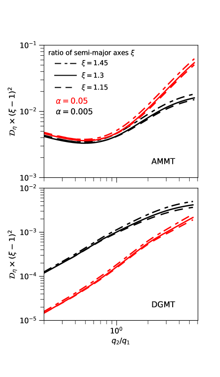
and . We found empirically that the combination , with given in Equation (9), varies little to changes in , implying that, in the range of under consideration, depends on as , in both AMMT and DGMT. This is shown in Figure 1, where we compare for three different values of . We took , and . Indeed, throughout this paper, we will take unless otherwise stated.
A clear difference between the models is that, for any value of , is significantly smaller in DGMT than in AMMT. Another difference is that, at fixed and , increases monotonically with in DGMT, whereas it presents a minimum at in AMMT.
The dependence of with in AMMT also differs from that in DGMT. In AMMT, for is larger than it is for , especially for . The reason is that the angular momentum deposited by the outer perturber decreases as its mass increases because it opens a deeper gap. However, DGMT predicts a reduction of the repulsive effect because radial gradients in the disk surface density induced by the companion become smaller as viscosity increases.
The repulsion mechanism is significant when . If we define as the ratio , and using the equation for derived in the Appendix C, and from Equation (8), the above condition implies:
| (10) |
Figure 2 shows versus for and different combinations of , and . For the brevity of the notation, we use the quantities . We consider values of that satisfy the following three conditions. First, the Hill condition (see Appendix D). The second condition is that the horseshoe regions are separated, i.e. , where is the half-width of the horseshoe region of orbiter . Finally, to justify the two-dimensional approximation, we demand that , where is the vertical scale height of the disk at , where .
As expected, decreases as the separation between the orbiters increases. For the parameters under consideration in Figure 2, in DGMT. In AMMT, the condition is fulfilled at .
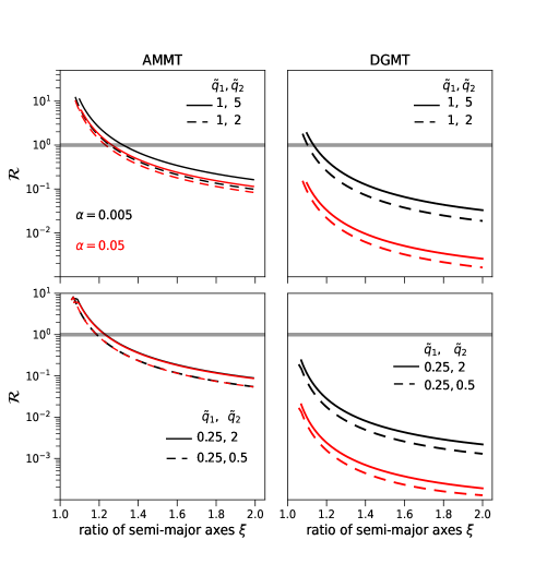
It is interesting to note that, for the case (corresponding to the bottom row of Fig. 2), the repulsive effect is a bit larger for than for , in both AMMT and DGMT. This result implies that although the inward migration rate of the outer perturber is larger for than for , this increase is correspondingly lower than the increase in the inward migration rate of the inner perturber.
AMMT predicts that when and are sufficiently small, is almost independent of (see lower left panel of Figure 2). The trend is different in DGMT; decreases as increases, even if and are small.
In the case that the inner body does not migrate because it is in a migration trap, the corresponding interaction offset is
| (11) |
and the condition is simplified to
| (12) |
We have checked that if all the parameters () are fixed, is significantly larger when both orbiters can migrate.
3 The simulations
In this section, we compute the disk forces acting on a pair of massive bodies embedded in a two-dimensional disk, using the publicly available code FARGO (Masset, 2000). We aim to explore the separations between the pair at which the repulsion effect is important and to test whether AMMT or DGMT can correctly predict the scaling and magnitude of . In order to isolate how the disk torques change in a disk already disturbed by its companion, the bodies are forced to move on fixed Keplerian orbits with orbital radii and , and eccentricities and (constant over time).
In all our models, the initial (unperturbed) radial profile of the surface density of the disk, , follows the power-law assumed in Section 2.2. For simplicity, is taken to be constant with and over time (locally isothermal disk) and can take one of two values: and . We will consider two values for ( and ) in our simulations. We limit ourselves to mass ratios . For this range of masses and the values of under consideration, the horseshoe regions of the orbiters do not overlap if .
To model the gravitational potential of the orbiters, we introduced a gravitational softening length . The forces on each perturber are calculated by summing the gravitational force in each grid cell. We use two tapering Gaussian functions to reduce the contribution of material bound to the orbiters
| (13) |
where and is the individual Hill radius of orbiter . Accretion onto the orbiters is not included in our simulations.
In code units, the inner boundary is located at and the outer boundary at , with wave-killing boundary conditions (de Val-Borro et al., 2006). In all the simulations with two perturbers, the initial semi-major axis of the inner orbiter is . The surface density of the disk is scaled so that the disk mass contained within is . In code units, and the orbital period is at . We measure the time in terms of the orbits revolved by a body at .
In all our simulations, the grid has (logarithmically spaced) and zones in the radial and azimuthal directions, respectively.
A certain model is specified by seven dimensionless parameters , , , , , and . Throughout this section, however, we use either or , with , and remind that is the vertical scale-height of the disk at . The relation between and is given by
| (14) |
3.1 Individual orbiter
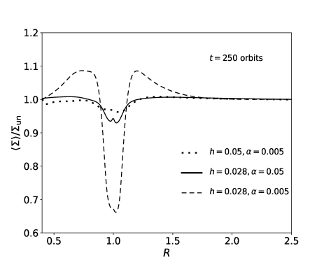
We start by considering the case where a single object with mass ratio is on a fixed circular orbit with semi-major axis . Figure 3 shows the ratio between the azimuthally-averaged surface density at orbits and the initial surface density, for different combinations of and . We see that the gap depth is small for and and and . However, for and , a partial gap () is carved in the disk. Since we restrict ourselves to models with , our orbiters open shallow or partial gaps when they are alone in the disk.
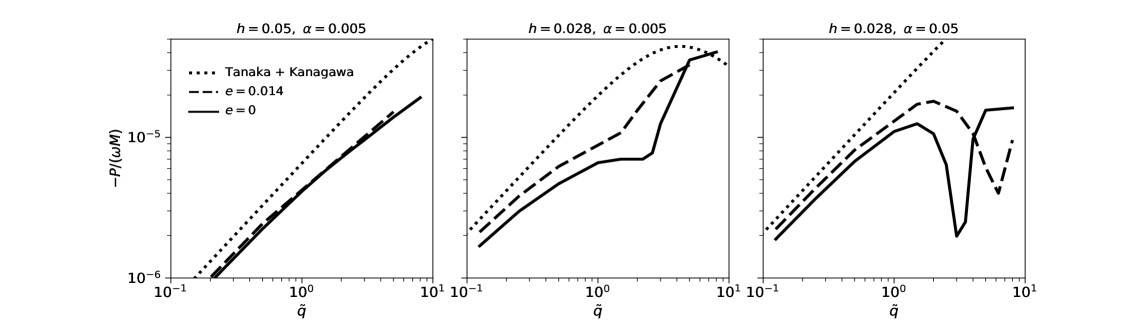
Figure 4 shows the steady-state magnitude of the specific power, more specifically , versus , for two orbital eccentricities. In the cases with and (left panel), is a monotonic function of . For and , presents a gap. The position of the gap in depends on the orbital eccentricity; it is located at for and at for . The origin of this gap in the torque in high-viscosity disks was already discussed in Masset et al. (2006).
3.2 Torques on a pair: Fixed circular orbits
In this section, we will focus on the particular case where the two components of the pair move on fixed circular orbits (, at any time) around the central object.
3.2.1 Temporal behaviour of
When two orbiters are immersed in the disk, the disk forces onto one of them display large variations in time because of the interaction with the perturbed density field created by the other one. Thus, we compute the torques using time averages over where is an integer and is the time between two successive passages of the orbiters through opposition (or synodic period):
| (15) |
We will use a bar over a quantity (e.g. and ) to denote its time-average over .
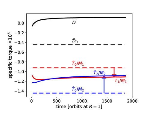
Figures 5 and 6 show representative examples of the temporal evolution of and , for and , respectively, in the circular case (). After sufficiently long times, and reach an almost constant value. We will denote these “steady-state” values with the subscript ss, e.g. , and .
For orbiters in circular orbits with separations , or in disks with , our simulations are long enough to reach a state where (and also the torques) is almost constant. Therefore, is computed as the value at those steady states. For the simulations with and , we ran the simulations to at least orbits. If the torques had not reached a steady-state value, we continued the simulations until varied less than for the last orbits. Then, we took as the value of at the end of the simulation.
3.2.2 versus
It is worthwhile to look again at Figures 5 and 6 to gain insight into the repulsion effect. In all cases, is more negative (the magnitude of the torque is larger) than it is when the orbiter is isolated (red horizontal lines). On the other hand, is always more positive than the torque when it is treated as a single body (blue horizontal lines). Therefore, the disk-mediated interaction between orbiters leads to a repulsive effect. Interestingly, in all cases presented in Figures 5 and 6, .
The interaction offset in the steady state, , can be computed in our simulations as , with calculated from Equation (3) in simulations where each orbiter is alone in the disk (as those computed in Section 3.1).
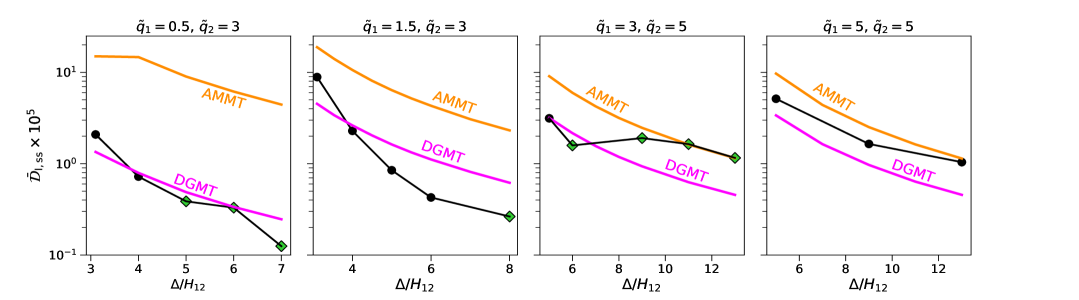
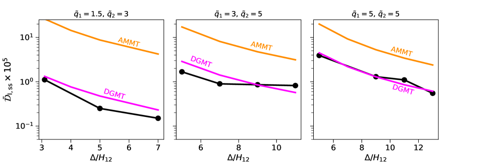
Figure 7 shows the dependence of on the orbital separation for different combinations of and . We have taken , and . In all cases shown in Figure 7, the maximum of occurs at the smallest value of considered. For these lowest values of , , implying that the migration would be divergent. In general, there is a trend for to decrease with the separation (see the left and middle-upper panels). However, it becomes almost constant between and in the third panel (for and ).
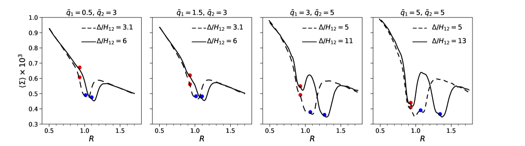
In Figure 8, we present the radial profile of the azimuthally-averaged surface density after orbits at , for two representative values of the orbital separation . We see that the orbiters share a common gap for . For the largest orbital separations explored, it is possible to distinguish the “individual” gaps (solid lines in the third and fourth panels). Note that the gap depths in the first and second panels are similar.
In Figure 7, we have also shown predicted in AMMT and DGMT described in Section 2 and Appendices A and B. We see that AMMT overestimates up to one order of magnitude in some cases. DGMT, on the other hand, can predict the value of within a factor of . It can also reproduce the slight ascend (from left to right-hand panels) of the curves from the simulations.
Figure 9 shows versus , as in Figure 7, but now for . We see that for and is generally smaller for than for . However, in the two models with and , for is quite similar to that for .
In the cases shown in Figure 9, AMMT overestimates and predicts that should be larger as viscosity increases, but the simulations do not show that trend. On the other hand, DGMT reasonably predicts the magnitude of the repulsive effect. A more comprehensive comparison between the results of simulations and the models will be presented in Section 3.2.4.
3.2.3 Dependence of the repulsion effect on and
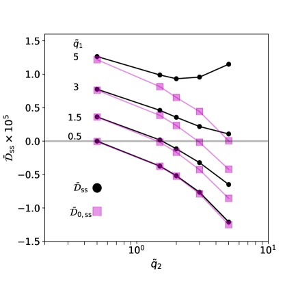
To see whether the orbiters can reverse the direction of migration from converging to diverging, it is worthwhile to compare with . Figure 10 shows and , both obtained from the simulations, for and , when (implying ). Along the curves, is varied, keeping constant. We see that for and for the values of under consideration, is rather similar to , meaning that the repulsion is small. The curves for and for essentially overlap for and separate from each other as increases. We find that for and , the disk-mediated interaction between orbiters should be taken into account, for separations . Yet for these values of and , the depth of the common gap is still very shallow. For instance, for , the depth of the gap is only .
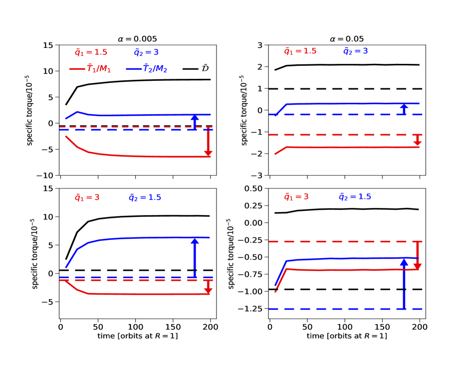
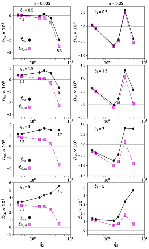
Figure 11 shows and for and . In this case, the semi-major axis ratio is very similar to the value adopted in Figure 10. We find that , implying that the effect is repulsive. increases as increases (fixed ) and as increases (fixed ). In some cases, , but .
Consider first the low viscosity disk (; left panels in Fig. 11). For , for any value of . In addition, for and , we have . In particular, if we take and , similar to those in Kepler-36 for illustration, we find that the migration is divergent if , provided that , and the orbits are circular.
In a disk with and (right panels in Fig. 11), the curves for exhibit a peak at ; this is reminiscent of the reduction of the torque for this value of the mass ratio (see Figure 4). also shows this peak but only when . For and , . Interestingly, for and , we have that (convergent migration), whereas (divergent migration).
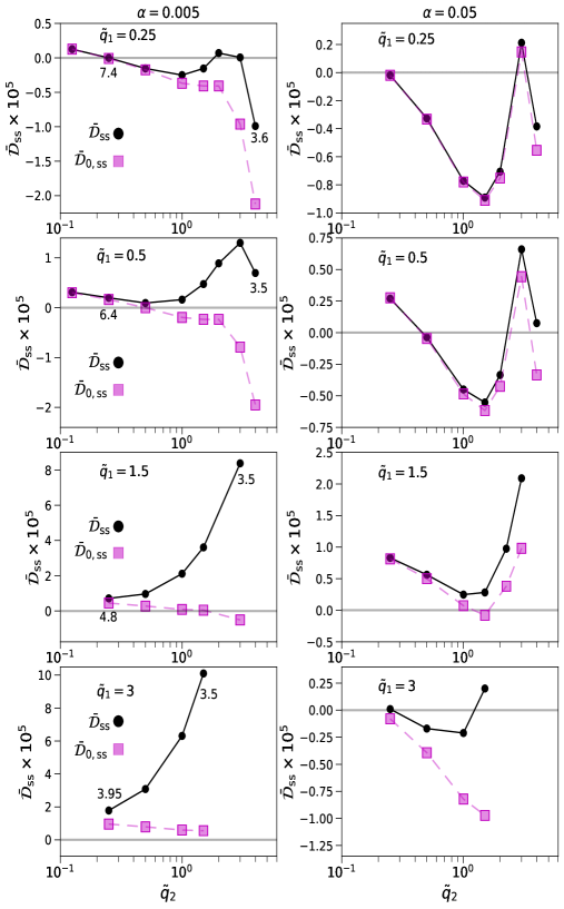
Figure 12 shows the results for , again for (for these parameters, ). Quite remarkably, even for the smallest inner mass considered in this figure, the repulsive effect is sufficiently strong to yield a divergent migration for , in the low viscosity case (). The migration is also divergent in all the models explored in that figure with and . For , and , migration switches from convergent to divergent because and .
Finally, we focus on models with (right panels in Figure 12). For , the shape of the curves for is rather similar to the shape of curves. However, for , the large discrepancy between and indicates that the disk-mediated interaction plays an important role.
3.2.4 Comparison with the predictions of AMMT and DGMT
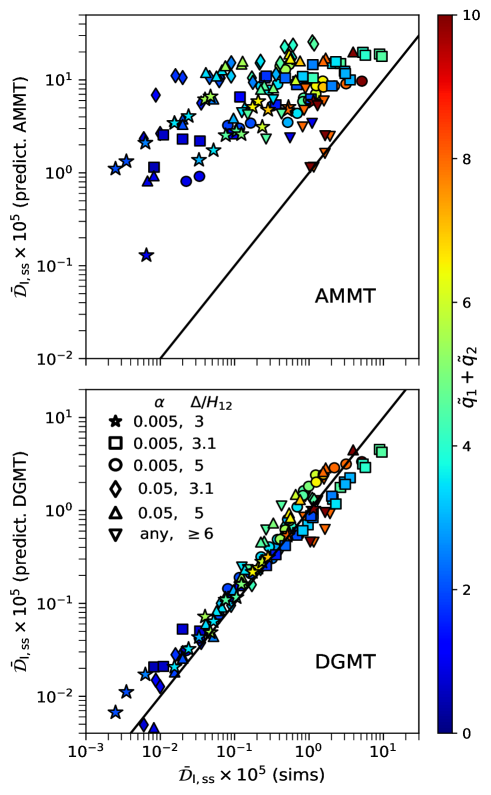
In Section 3.2.2, we already mentioned that, for the cases considered in that section, DGMT is more consistent with the results of simulations than AMMT, as AMMT generally overestimates the magnitude of . This is confirmed in Figure 13 where we show a one-to-one comparison between the predicted values of and those obtained from the simulations. We see that AMMT fails to predict the scalings of and, in addition, overestimates for orbital separations . However, DGMT correctly captures the scaling of with , , , and radial separation . When , the simulations show a mildly weaker effect than predicted by DGMT. This has a simple explanation. The time scale to reach a steady state is orbits for , and orbits for (e.g., Ataiee et al., 2018). For , the time is a bit longer than the running times of our simulations. This is particularly true for low-mass perturbers () in a disk with and (the three star symbols at the bottom left corner of Figure 13), for which our simulations were not long enough to establish a steady state. As a consequence, the variations of the slope of surface density have not reached their steady state values, hence numerical simulations show a repulsion weaker than predicted. On the other hand, the scatter in the upper part of the diagram (at values ) may reflect the fact that the analytical model for the gap profile given by Equation (B4), as well as the expression for the corotation torque in Equation (B1) used to compute in DGMT become less accurate for masses larger than the thermal mass ().
3.3 Eccentric orbits
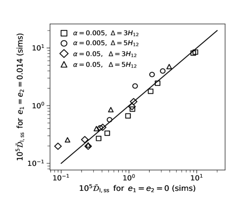
In the previous section, we assumed that the orbiters have null eccentricities. However, the gravitational interaction between the pair’s components will excite their eccentricities. Therefore, it is worthwhile to see how sensitive is to the orbiters’ eccentricities. To do so, we have conducted the following test. For a subset of the simulations shown in Figs. 11 and 12, we have redone the simulations with the same parameters but adopting for the orbital eccentricities of the perturbers, which were kept constant throughout the duration of the runs. We ran the models for the same number of orbits as we did in their circular counterparts and computed as the average of over the last complete oscillations (typically orbits). Since the shape of the radial profile of the gaps open by individual orbiters with is rather similar to that for individual orbiters in a circular orbit, we expect that DGMT will be for these eccentric pairs as accurate as for circular pairs. Figure 14 compares as obtained in the simulations with with the values in simulations having . We see that may differ by up to for the models under consideration. In summary, as long as the orbital eccentricities are moderate (), hardly changes by a factor larger than as compared to the case where the eccentricities are fixed to zero.
4 Discussion: why does AMMT yield wrong results?
In Section 3.2.4 we have found that AMMT generally overestimates the effect of repulsion, implying that the orbiters absorb less angular momentum than the amount deposited in their horseshoe regions. Here, we present a simple simulation that clearly shows that the excess torque on the orbiter is not that deposited in the disk within its horseshoe region. More specifically, we conducted a simulation of the outer orbiter alone in the disk but applying an imposed (external) positive torque density, , to the disk. This external torque imitates the torque deposited by the inner orbiter. To avoid spurious changes in the surface density due to the imposed torque, we require that the specific torque scales with as , where is the second Oort constant, with the disk orbital frequency (Masset & Papaloizou, 2003). In the absence of the orbiter, this torque induces a constant outward drift in a disk with a stationary axisymmetric density profile . In this particular choice of , no waves are excited by the external torque.
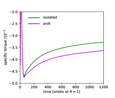
We have computed the torque on an orbiter with at , in a simulation where it is isolated in the disk (with and ), and in a simulation where the effect of the inner orbiter has been replaced by , with (in code units) at . This magnitude of the external torque density corresponds to the torque density deposited at by the damping of the wake excited by an inner orbiter with at , when alone in the disk. It was measured in the simulations of a single orbiter, as , where is the angular momentum flux carried by the waves, which is given by
| (16) |
where and are the radial and azimuthal components of the gas velocity, respectively, and the bar indicates the azimuthal average. We comment that this procedure neglects a potential excitation term (by the inner perturber) at the orbit of the outer perturber. The ratio of orbital radii between the outer and inner perturber is and the ratio of orbital periods is , which indicates that all the outer Lindblad resonances of the inner perturber are located inside of the outer perturber’s orbit, except that of the Fourier component of the inner planets’ potential, which lies outside. The residual excitation that may take place over the width of the horseshoe region should therefore represent a tiny fraction of incident flux of angular momentum, especially in a disc as thin as the one considered in this experiment. Furthermore, these considerations about the magnitude of the deposition of angular momentum within the horseshoe region will soon appear futile, as the torque excess on the outer orbiter does not even match the sign of the torque deposited.
Figure 15 shows the torques as a function of time. According to AMMT, the magnitude of the torque acting on the outer orbiter should be augmented by an amount of (evaluated at ) with respect to the isolated case. This implies an offset in the specific torque of if . This result is in sharp contrast with the outcomes of the simulation with , where we see that the torque presents an offset of after orbits (the torque is more negative than it is when the orbiter is isolated in the disk; see magenta and green curves in Fig. 15). However, this result is in agreement with studies of type III migration, where the relative planet-disk drift is achieved by inducing a disk drift under the action of external torque. The torque applied to the disk entails an outward drift. This is equivalent to a situation where the disk does not drift, and the planet migrates inwards. If the horseshoe region is partially depleted, as is the case here, type III torques arise and exert a positive feedback on migration (Masset & Papaloizou, 2003), i.e. they tend to make the negative torque larger in absolute value. This is precisely what we see in Fig. 15. This goes against the expectation that the torque on the orbiter due to the action of the external torque can be evaluated by calculating the angular momentum given to the disk within its horseshoe region. While it is true that fluid elements trapped in the horseshoe region ultimately transmit the positive torque deposited to the orbiter, fluid elements flowing (outwards) through the horseshoe region extract angular momentum from the orbiter during their unique horseshoe U-turn with the latter. The net effect is an increase in the absolute value of the torque.
The standard AMMT scenario contemplates only the contribution from within the horseshoe region and arbitrarily discards the effect of material immediately interior to that region that flows towards the outer disk. By construction, this scenario yields a torque excess that has the correct sign, but it cannot have the correct value, as it considers only half of the problem.
5 Summary
In this work, we have re-examined the repulsion effect in packed pairs in cases where the pair components carve partial gaps in the disk (). We focus on cases where the total mass of the pair is . In the case of protoplanetary disks, this corresponds to sub-Neptune-mass planets. In the case of AGN disks, this corresponds to the so-called extreme mass ratio inspirals (EMRIs). It includes an inspiral formed by BHs in an accretion disk around a central massive BH.
We have used as a measure of the repulsion effect. We have developed a semi-analytical framework to provide a quantitative view of the scalings of with the orbiters’ mass, orbital separation, disk aspect ratio, and viscosity. We applied two different assumptions: AMMT and DGMT. AMMT assumes that the torques are modified because each orbiter absorbs the angular momentum deposited on its horseshoe region by the wakes excited by its respective companion. DGMT assumes that the corotation torques are modified because the companion modifies the surface density profile of the disk. The formulation can also be applied when the inner orbiter does not migrate if it is in a migration trap.
We have measured in two-dimensional simulations of a pair of orbiters in fixed orbits for a wide range of orbiters’ mass ratios (), and disk viscosity (a variation of a factor of ). The magnitude of spans nearly three orders of magnitude. We have confirmed, in agreement with previous results, that (1) high-mass orbiters present a larger repulsion effect than low-mass orbiters, (2) the repulsive effect may be large enough to stall convergent migration, regardless of whether the pair is close or not to resonance, and (3) the repulsion effect decreases as the disk viscosity is increased. In most of our simulations, we forced the perturbers to be on circular orbits. Nevertheless, we have also explored orbits with eccentricities of and found similar repulsion.
We have compared the predictions of AMMT and DGMT with the results of the hydrodynamical simulations. AMMT is incapable of reliably predicting the scaling of with , , and . In particular, for our adopted range of parameters, AMMT generally overestimates the magnitude of the wake-orbiter interaction by up to two orders of magnitude, especially in disks with high viscosity.
We find that a more robust approach is DGMT, which can successfully account for the scaling of , at least for the range of parameters explored in this paper. Note that this work focuses exclusively on the repulsion effect due to the forces mediated by the disk, ignoring the mutual gravitational interaction between the pair components, which can be strong, especially when the planets are near first-order commensurabilities.
References
- Ataiee et al. (2018) Ataiee, S., Baruteau, C., Alibert, Y., Benz, W. 2018, A&A, 615, A110
- Ataiee & Kley (2021) Ataiee, S., Kley, W. 2021, A&A, 648, A69
- Baruteau & Masset (2013) Baruteau, C., Masset F. 2013, Tides in Astronomy and Astrophysics, Lecture Notes in Physics, Vol. 861, ed J. Souchay, S. Mathis and T. Tokieda (Berlin: Springer Verlag), 201
- Baruteau & Papaloizou (2013) Baruteau, C., Papaloizou, J. C. B. 2013, ApJ, 778, 7
- Bellovary et al. (2016) Bellovary, J. M., Mac Low, M.-M., McKernan, B., Ford, K. E. S. 2016, ApJL, 819, L17
- Charalambous et al. (2022) Charalambous, C., Teyssandier, J., Libert, A.-S. 2022, MNRAS, 514, 3844
- Choksi & Chiang (2020) Choksi, N., Chiang, E. 2020, MNRAS, 495, 4192
- Crida et al. (2006) Crida, A., Morbidelli, A., & Masset, F. 2006, Icarus, 181, 587
- Cui et al. (2021) Cui, Z., Papaloizou, J. C. B., Szuszkiewicz, E. 2021, ApJ, 921, 142
- de Val-Borro et al. (2006) de Val-Borro, M., Edgar, R. G., Artymowicz, P., et al. 2006, MNRAS, 370, 529
- Duffell (2015) Duffell, P. C. 2015, ApJ, 807, L11
- Fabrycky et al. (2014) Fabrycky, D. C. et al., 2014, ApJ, 790, 146
- Ginzburg & Sari (2018) Ginzburg, S., Sari, R. 2018, ApJ, 479, 1986
- Gladman (1993) Gladman, B. 1993, Icarus, 106, 247
- Goldreich & Tremaine (1979) Goldreich, P., Tremaine, S. 1979 ApJ, 233, 857
- Goodman & Rafikov (2001) Goodman, J., Rafikov, R. R. 2001, ApJ, 552, 793
- Izidoro et al. (2017) Izidoro, A., Ogihara, M., Raymond, S. N., et al. 2017, MNRAS, 470, 1750
- Jiménez & Masset (2017) Jiménez, M. A., Masset, F. S. 2017, MNRAS, 471, 4917
- Kanagawa et al. (2018) Kanagawa, K. D., Tanaka, H., Szuszkiewicz, E. 2018, ApJ, 861, 140
- Kanagawa & Szuszkiewicz (2020) Kanagawa, K. D., Szuszkiewicz, E. 2020, ApJ, 894, 59
- Kocsis, Yunes & Loeb (2011) Kocsis, B., Yunes, N., Loeb, A. 2011, PhRvD, 84, 024032
- Lissauer et al. (2011) Lissauer, J. J., Ragozzine, D., Fabrycky, D. C., et al. 2011, ApJS, 197, 8
- Lithwick & Wu (2012) Lithwick, Y., Wu, Y. 2012, ApJ, 756, L11
- Masset (2000) Masset, F. 2000, A&AS, 141, 165
- Masset (2002) Masset, F. S. 2002, A&A, 387, 605
- Masset & Casoli (2010) Masset, F. S., Casoli, J. 2010, ApJ, 723, 1393
- Masset et al. (2006) Masset, F. S., D’Angelo, G., & Kley, W. 2006, ApJ, 652, 730
- Masset & Papaloizou (2003) Masset, F. S., Papaloizou, J. C. B. 2003, ApJ, 588, 494
- McKernan et al. (2011) McKernan, B., Ford, K. E. S., Lyra, W., Perets, H. B., Winter, L. M., Yaqoob, T. 2011, MNRAS, 417, L103
- McKernan et al. (2020) McKernan, B., Ford, K. E. S., O’Shaugnessy, R., Wysocki, D. 2020, MNRAS, 494, 1203
- Nelson (2018) Nelson, R. P. Handbook of Exoplanets, ed. H. J. Deeg & J. A. Belmonte (Berlin: Springer), 139
- Paardekooper et al. (2010) Paardekooper, S.-J., Baruteau, C., Crida, A., Kley, W. 2010, MNRAS, 401, 1950
- Podlewska-Gaca et al. (2012) Podlewska-Gaca, E., Papaloizou, J. C. B., Szuszkiewicz, E. 2012, MNRAS, 421, 1736
- Rafikov (2002) Rafikov, R. R. 2002, ApJ, 572, 566
- Rowan et al. (2023) Rowan, C., Boekholt, T., Kocsis, B., Haiman, Z. 2023, MNRAS, 524, 2770
- Secunda et al. (2019) Secunda, A., Bellovary, J., Mac Low, M.-M., Ford, K. E. S., McKernan, B., Leigh, N. W. C., Lyra, W., Sándor, Z. 2019, ApJ, 878, 85
- Tanaka et al. (2002) Tanaka, H., Takeuchi, T., Ward, W. R. 2002, ApJ, 565, 1257
- Ward (1991) Ward, W. R. 1991, Lunar Planet. Sci. Conf., 22, 1463
- Ward (1992) Ward, W. R. 1992, Lunar Planet. Sci. Conf., 23, 1491
- Yang et al. (2019) Yang, Y., Bartos, I., Haiman, Z., Kocsis, B., Márka, Z., Stone, N. C., Márka, S. 2019, ApJ, 876, 122
Appendix A and in the AMMT assumption
In this Appendix, we derive the angular momentum deposited in the horseshoe regions. The angular momentum flux excited by orbiter can be written as , with the dimensionless angular momentum flux. For isolated perturbers that do not open deep gaps, can be found in Rafikov (2002) (see also Goodman & Rafikov, 2001). It can be approximated by:
| (A1) |
where is the dimensionless wave-to-shock timescale (see Rafikov (2002) for details), given by
| (A2) |
and
| (A3) |
We recall that is the power-law exponent of the unperturbed surface density of the disk. The fraction of the angular momentum excited by the perturber that is deposited in the horseshoe region of perturber is
| (A4) |
where , with the half-width of the horseshoe region.
In principle, the deposition torque depends on the surface density profile of the disk. Equations (A1)-(A4) assume that the radial profile of the surface density follows a power-law and ignore the fact that the companion could open a gap that modifies the underlying structure of the disk. For perturbers that open partial gaps, this non-linear effect is likely small (e.g., Ginzburg & Sari, 2018).
Following Cui et al. (2021), we will assume that the perturber can absorb the angular momentum deposited in its horseshoe region if it is less than the one-sided horseshoe drag . Using that , the condition implies:
| (A5) |
and
| (A6) |
Appendix B and in the DGMT assumption
In this Appendix, we compute the change in the corotation torque as the companion modifies the disk surface density.
The unsaturated corotation torque on perturber in the steady state case, when it is alone in the disk on a fixed circular orbit, is given by
| (B1) |
where is the second Oort’s constant (Goldreich & Tremaine, 1979; Ward, 1991, 1992). This formula is valid if the perturber does not open a deep gap in the disk. In order to take into account that the corotation torque may differ from the unsaturated value because it can be partially saturated, we include a correction factor , so that . The correction factor depends on , the ratio between the libration timescale and diffusion timescale across the horseshoe region. For , we take from Masset & Casoli (2010):
| (B2) |
where is defined by Eq. (120) of Masset & Casoli (2010). For , we take the values reported in the Figure 12 of the same paper.
If, in the presence of the companion, the surface density profile changes from to , the change in the corotation torque will be
| (B3) | |||||
where we have assumed that the rotation of the disk is Keplerian (i.e. ). From Duffell (2015), we know that
| (B4) |
with and as given in Equation (A1). Using our definition of and recalling that , we obtain
| (B5) |
A similar procedure can be followed to derive . We get
| (B6) |
Here is given by Equation (B4) but replacing the subscript with . In the cases of interest, and are both positive, so the effect is generally repulsive. As expected, and are proportional to the fourth power of and , respectively. Thus, to predict correctly the magnitude of and , it is important to have a precise value for . The procedure to compute in our simulations is described in the Appendix E.
In principle, the differential Lindblad torque on each orbiter will also be modified if the structure of the disk changes due to the presence of the companion. We note, however, that the dependence of the Lindblad torque on the slope of surface density is much weaker than that of the corotation torque, not only in a realistic, 3D disk (Tanaka et al., 2002), but also in the 2D disks considered in this paper, even for the low-mass planets for which the width of the horseshoe region is not enhanced (see Appendix E). In fact, Paardekooper et al. (2010) showed that the differential Lindblad torque, , on perturber (alone in the disk) in circular orbit in a 2D disk with constant is given by
| (B7) |
with . From the above equation and for the smoothing length used in this work, the change in the differential Lindblad torque when the background density is modified to is
| (B8) |
We may compare given in Equation (B3) with , assuming, for simplicity, that the outer perturber opens a Gaussian gap so that , where is the depth of the gap and its width. By combining Eqs. (B3) and (B8), it is simple to show that
| (B9) |
To derive this equation, we have taken conservatively that in Equation (B3). For and the values of considered in this paper, we find that . A similar argument leads to . It is therefore legitimate to neglect the Lindblad torque in the DGMT scenario.
Appendix C Two independent migrators
In this section, we estimate defined as , given in Equation (3), when the bodies are so far apart that the torques they experience are not affected by the presence of their companion. The torque exerted on an isolated migrator in a steady state, i.e. when the gap has become a steady-state structure, was computed by Kanagawa et al. (2018), using two-dimensional hydrodynamical simulations. For , they find that the torque exerted on a migrator that opens a partial gap is approximately given by the Type I migration formula but replacing the disk surface density by the surface density at the bottom of the gap (see Figure 7 in Kanagawa et al. 2018111Note that the points are scattered around the values predicted by this relationship. As discussed by Kanagawa et al. (2018), the torque can even be positive in some cases. For the combinations of parameters chosen in this paper, this relationship overestimates (see Section 3.1).). From Duffell (2015), we have , where is given in Equation (7). On the other hand, we may use the formula for the Type-I torque from Tanaka et al. (2002) to obtain , with in a two-dimensional disk. Combining these equations, we find from Equation (3):
| (C1) |
Therefore, if and are constant along the disk and then and, consequently, remains constant over time (see Eq. 2). On the other hand, the migration is divergent if , while it is convergent if .
Appendix D Hill stability condition
Assume that initially, the orbiters are on circular orbits and focus on pairs satisfying the condition for Hill stability. In the absence of the accretion disk, the pair is said to be Hill stable if the gravitational interactions between the two orbiters remain moderate. The Hill stability condition is commonly written in terms of the mutual Hill radius, defined as:
| (D1) |
where and . In the case of initially circular orbits, Gladman (1993) showed that the condition , where , ensures Hill stability because close encounters between the orbiters are forbidden. Even though the interaction between the orbiters may lead to episodes where their eccentricities can increase, conservation of angular momentum (if the disk is not present) implies that the orbital separation increases, impeding close encounters. In terms of , Gladman’s condition implies
| (D2) |
For instance, for , it implies .
Appendix E The half-width of the horseshoe region in our simulations
Since some planets in our samples have a mass near or slightly above the thermal mass , the standard, low-mass estimate for the width of the horseshoe region may lead to an underestimation of the variation of the corotation torque. It is, therefore, desirable to use a formula for the width of the horseshoe region that captures the transition from the low- to the high-mass regime. Jiménez & Masset (2017) have studied this transition, but their results apply to planets in three-dimensional disks. Here, we have planets in two-dimensional disks and a smoothing length of the potential of , for which no result exists in the literature. We have therefore undertaken a dedicated study similar to that of Jiménez & Masset (2017), but in 2D disks with the smoothing length quoted above. We performed 20 runs over 10 orbital periods, with planet masses ranging from to in a geometric sequence, in an inviscid disk with aspect ratio . The resolution adopted in these runs was and , the radial bins having a constant spacing covering the range to (the planet’s orbital radius being one). The half-width of the horseshoe region is then obtained as the mean of the rear and front upstream half-widths, measured at from the azimuth of the planet. Following Jiménez & Masset (2017), expressing the planet’s mass in units of the thermal mass () and the half-width of the horseshoe region in units of the pressure lengthscale (), we obtain the following regimes:
| (E1) | |||
| (E2) |
At any given mass, we find that the horseshoe half width is within %, at most, of the linear combination of these two extreme regimes given by:
| (E4) |
where . From this we infer the value used in Appendices A and B.