Investigating Training Objectives for
Generative Speech Enhancement

Abstract

Generative speech enhancement has recently shown promising advancements in improving speech quality in noisy environments. Multiple diffusion-based frameworks exist, each employing distinct training objectives and learning techniques. This paper aims at explaining the differences between these frameworks by focusing our investigation on score-based generative models and Schrödinger bridge. We conduct a series of comprehensive experiments to compare their performance and highlight differing training behaviors. Furthermore, we propose a novel perceptual loss function tailored for the Schrödinger bridge framework, demonstrating enhanced performance and improved perceptual quality of the enhanced speech signals. All experimental code and pre-trained models are publicly available to facilitate further research and development in this domain.

I Introduction

Diffusion-based generative models have been successfully employed in various audio restoration tasks, most notably in speech enhancement [1]. Generative methods in this task aim at estimating and sampling from the clean speech distribution conditioned on noisy speech. Unlike predictive models, generative models enable the generation of multiple valid estimates for a given input and can be utilized for generalized (or universal) speech enhancement, effectively addressing various corruption types [2].

Numerous diffusion-based generative approaches exist, all centered around the idea of defining a transformation between the data distribution and a tractable prior distribution (e.g., Gaussian). Popular frameworks include continuous-time diffusion models [3], EDM [4], flow matching [5], and Schrödinger bridge (SB) [6]. Each of these approaches has been applied to speech enhancement.

SGMSE [7, 8] is the first work that employs continuous-time diffusion models based on stochastic differential equations. Follow-up work utilizes the EDM framework; it has been proposed to use a change of variable to consider the SDE satisfied by the environmental noise [9], which results in the required linear affine drift term. Flow matching has been used in SpeechFlow [10], where the authors apply masked audio prediction as a self-supervised pretraining technique.

More recently, SB has been proposed for speech enhancement [11]. The SB is a generative model that seeks an optimal way to transport one probability distribution to another distribution [6]. This approach enables starting the generative process directly from the noisy input and allows for using a data prediction loss [12].

This paper builds upon the above-mentioned advances and explores multiple training objectives and learning techniques for generative speech enhancement. We begin by exploring score-based generative models and connect various loss functions used to learn the score function. For further details, we refer to [13], showing how various diffusion-based generative model objectives can be understood as special cases of a weighted loss. Second, we examine the SB approach for speech enhancement [11] and establish a connection to score-based generative models for speech enhancement (SGMSE) [8]. Moreover, we propose a novel perceptual loss function for the SB framework and perform ablation studies to evaluate its effect. Specifically, drawing inspiration from the PESQetarian [14], we introduce a loss term based on the PESQ metric [15].

Our experiments demonstrate that score-based generative models trained with different objective functions exhibit varying training behaviors, although they theoretically model the same underlying concepts. We hypothesize this is due to the neural network’s different training tasks. Additionally, we show that our novel perceptual loss for the SB achieves state-of-the-art performance in PESQ on the Voiceband-Demand (VB-DMD) benchmark [16].

Contemporaneously to our work, Wang et al. [17] explore the SB and set a symmetric noise scheduling, where the diffusion shrinks at both boundaries. Furthermore, they combine the SB concept with a two-stage approach inspired by StoRM [18], utilizing a predictive model to aid generative models with a magnitude ratio mask.

The paper is structured as follows: Sec. II explores SGMSE and the SB framework. This is followed by describing the experimental setup in Sec. III. Then, we present the results of the experiments in Sec. IV. Finally, in Sec. V, we summarize our key findings and provide an outlook on future work.

II Methods

This section discusses two existing generative approaches for speech enhancement and explores their connection. First, we introduce SGMSE [8]. Second, we examine the SB for speech enhancement [11]. Both approaches are diffusion-based stochastic processes aiming to model and manipulate probability distributions. Score-based models emphasize learning score functions, whereas the SB approach can be considered as an optimal transport problem.

II-A Score-based generative models for speech enhancement

Following [8], the diffusion forward process is described by the solution to the forward SDE

$$\mathrm{d}\mathbf{x}_{t}=\gamma(\mathbf{y}-\mathbf{x}_{t})\mathrm{d}t+g(t)\mathrm{d}\mathbf{w},$$ (1)

where $\mathbf{x}_{t}\!\in\!\mathbb{C}^{d}$ is the process state at time $t\!\in\!\left[0,1\right]$ and $\mathbf{y}\!\in\!\mathbb{C}^{d}$ is the noisy speech. The diffusion coefficient $g(t)=\sqrt{c}k^{t}$ controls the Gaussian noise introduced by the Wiener process $\mathbf{w}\!\in\!\mathbb{C}^{d}$. Moreover, $\gamma$, $c$, and $k$ are positive scalar constants that are set as hyperparameters. The forward process is also called Ornstein-Uhlenbeck process with variance exploding (OUVE) SDE[19].

The marginals of the time-reversed forward process can be represented as marginals of another stochastic process (see Theorem A.1 in [20]). This resulting process is described by the solution to the so-called reverse SDE

$$\mathrm{d}\mathbf{x}_{t}=\left[-\gamma(\mathbf{y}-\mathbf{x}_{t})+g(t)^{2}\nabla_{\mathbf{x}_{t}}\log p_{t}(\mathbf{x}_{t}|\mathbf{y})\right]\mathrm{d}t+g(t)\mathrm{d}\bar{\mathbf{w}}\,,$$ (2)

where $\nabla_{\mathbf{x}_{t}}\log p_{t}(\mathbf{x}_{t}|\mathbf{y})$ is the conditional score function, and $\bar{\mathbf{w}}$ is the Wiener process backward in time.

It can be shown that the OUVE SDE results in an interpolation between clean speech $\mathbf{x}_{0}$ and noisy speech $\mathbf{y}$ with exponentially increasing variance [8]. The evolution of the marginals is described by the time-dependent mean

$$\bm{\mu}_{t}(\mathbf{x}_{0},\mathbf{y})=e^{-\gamma t}\mathbf{x}_{0}+(1-e^{-\gamma t})\mathbf{y}$$ (3)

and the time-dependent variance

$$\sigma_{t}^{2}=\frac{c(k^{2t}-e^{-2\gamma t})}{2(\gamma+\log k)}\,,$$ (4)

that allow for direct sampling of the process state $\mathbf{x}_{t}$ at time $t$ using the perturbation kernel

$$p_{0t}(\mathbf{x}_{t}|\mathbf{x}_{0},\mathbf{y})=\mathcal{N}_{\mathbb{C}}(\mathbf{x}_{t};\bm{\mu}_{t}(\mathbf{x}_{0},\mathbf{y}),\sigma_{t}^{2}\mathbf{I})\,.$$ (5)

The score function is typically intractable and approximated by a score model $\mathbf{s}_{\theta}$ with parameters $\theta$. To train the score model, we use the denoising score-matching objective [21]

$$\mathcal{L}_{\text{DSM}}=\lambda(t)\lVert\mathbf{s}_{\theta}(\mathbf{x}_{t},\mathbf{y},t)-\nabla_{\mathbf{x}_{t}}\log p_{0t}(\mathbf{x}_{t}|\mathbf{x}_{0},\mathbf{y})\rVert_{2}^{2}$$ (6)

where $\lambda(t)$ is a weighting function, and the other variables are sampled according to $t\sim\mathcal{U}[0,1]$, $(\mathbf{x}_{0},\mathbf{y})\sim p_{\text{data}}(\mathbf{x}_{0},\mathbf{y})$ from the dataset, and $\mathbf{x}_{t}\sim p_{0t}(\mathbf{x}_{t}|\mathbf{x}_{0},\mathbf{y})$. The score matching loss is essentially equivalent to a noise prediction loss

$$\mathcal{L}_{\text{score}}=\lVert\mathbf{s}_{\theta}(\mathbf{x}_{t},\mathbf{y},t)\,\sigma_{t}+\mathbf{z}\rVert_{2}^{2}~{}\text{,}$$ (7)

when $\lambda(t)=\sigma_{t}^{2}$ in Eq. (6), and $\mathbf{z}\sim\mathcal{N}(\mathbf{0},\mathbf{I})$. To improve numerical stability, the output of an employed neural network $F_{\theta}$ is often scaled by a factor of $1/\sigma_{t}$ such that $\mathbf{s}_{\theta}(\mathbf{x}_{t},\mathbf{y},t)=F_{\theta}(\mathbf{x}_{t},\mathbf{y},t)/\sigma_{t}$.

Following the derivations in [4], it can also be shown that denoising score matching for SGMSE is equivalent to training a denoiser model $D_{\theta}$ with the denoising loss

$$\mathcal{L}_{\text{denoise}}=\lambda(t)\lVert D_{\theta}(\mathbf{x}_{t},\mathbf{y},t)-\bm{\mu}_{t}(\mathbf{x}_{0},\mathbf{y})\rVert^{2}_{2}\,.$$ (8)

Furthermore, it was argued that it is beneficial to precondition a neural network $F_{\theta}$ to obtain the denoiser

$$D_{\theta}(\mathbf{x}_{t},\mathbf{y},t)=c_{\text{skip}}(t)\mathbf{x}_{t}+c_{\text{out}}(t)F_{\theta}\big{(}c_{\text{in}}(t)\mathbf{x}_{t},\,c_{\text{in}}(t)\mathbf{y},\,t\big{)}$$ (9)

where $c_{\text{skip}}(t)$, $c_{\text{out}}(t)$, $c_{\text{in}}(t)$, and $c_{\text{in}}(t)$ are time-dependent functions that can be derived from first principles (see Appendix B.6 in [4]). Then, the score is then given by

$$\mathbf{s}_{\theta}(\mathbf{x}_{t},\mathbf{y},t)=\frac{D_{\theta}(\mathbf{x}_{t},\mathbf{y},t)-\mathbf{x}_{t}}{\sigma_{t}^{2}}\,.$$ (10)

II-B Schrödinger bridge for speech enhancement

The SB [22] is defined as the minimization of the Kullback-Leibler divergence $D_{\text{KL}}$ between a path measure $p$ and a reference path measure $p_{\text{ref}}$, subject to boundary conditions

$$\min_{p\in\mathcal{P}_{\left[0,1\right]}}D_{\text{KL}}\left(p,p_{\mathrm{ref}}\right)\quad\text{s. t.}\quad p_{0}=p_{x},\thickspace p_{1}=p_{y},$$ (11)

where $\mathcal{P}_{\left[0,1\right]}$ is the space of path measures on $\left[0,1\right]$ [6]. An optimal transport solution is given by a pair of symmetric forward and reverse SDEs, with the forward SDE being

$$\mathrm{d}\mathbf{x}_{t}=\left[\mathbf{f}(\mathbf{x}_{t})+g(t)^{2}\nabla_{\mathbf{x}_{t}}\log\Psi_{t}(\mathbf{x}_{t})\right]\mathrm{d}t+g(t)\mathrm{d}\mathbf{w}_{t},\,\mathbf{x}_{0}\sim p_{x},$$ (12)

and the reverse SDE being

$$\mathrm{d}\mathbf{x}_{t}=\left[\mathbf{f}(\mathbf{x}_{t})-g(t)^{2}\nabla_{\mathbf{x}_{t}}\log\bar{\Psi}_{t}(\mathbf{x}_{t})\right]\mathrm{d}t+g(t)\mathrm{d}\bar{\mathbf{w}}_{t},\,\mathbf{x}_{1}\sim p_{y},$$ (13)

where the functions $\Psi_{t},\bar{\Psi}_{t}$ are described by coupled partial differential equations (see Theorem 1 in [6])

$$\begin{cases}\frac{\partial\Psi_{t}}{\partial t}=-\nabla_{\mathbf{x}_{t}}\bar{\Psi}_{t}(\mathbf{x}_{t})^{\text{T}}\mathbf{f}(\mathbf{x}_{t})-\frac{1}{2}\operatorname{Tr}\left(g(t)^{2}\nabla_{\mathbf{x}_{t}}^{2}\Psi_{t}(\mathbf{x}_{t})\right)\\ \frac{\partial\bar{\Psi}_{t}}{\partial t}=-\nabla_{\mathbf{x}_{t}}\cdot(\bar{\Psi}_{t}(\mathbf{x}_{t})\mathbf{f}(\mathbf{x}_{t}))+\frac{1}{2}\operatorname{Tr}\left(g(t)^{2}\nabla_{\mathbf{x}_{t}}^{2}\bar{\Psi}_{t}(\mathbf{x}_{t})\right)\end{cases}$$

$$\textit{s.t.}\,\,\Psi_{0}\bar{\Psi}_{0}=p_{x},\Psi_{1}\bar{\Psi}_{1}=p_{y}.$$ (14)

However, for a system of symmetric forward and reverse SDEs in Eqs. (12, 13), and arbitrary $\Psi_{t}$ and $\bar{\Psi}_{t}$, there are infinitely many solutions bridging the prior to the target [23]. According to Nelson’s identity [24]

$$\nabla_{\mathbf{x}_{t}}\log\Psi_{t}(\mathbf{x}_{t})+\nabla_{\mathbf{x}_{t}}\log\bar{\Psi}_{t}(\mathbf{x}_{t})=\nabla_{\mathbf{x_{t}}}\log p_{t}(\mathbf{x}_{t}),$$ (15)

which is a necessary condition for time-reversal [23], we note that in score-based generative models, this corresponds to setting $\nabla_{\mathbf{x}_{t}}\log\Psi_{t}$ to zero. This implies that in score-based generative models, the drift of the forward process, e.g., $\mathbf{f}_{\text{SGMSE}}(\mathbf{x}_{t})=\gamma(\mathbf{y}-\mathbf{x}_{t})$ in Eq. (1), has to be chosen such that the perturbation kernel is known analytically. However, this is not required for the general SB formulation.

Although solving the general SB is typically intractable, closed-form solutions are available for specific cases, such as those involving Gaussian boundary conditions [25]. Assume a drift $\mathbf{f}(\mathbf{x}_{t})\!=\!f(t)\,\mathbf{x}_{t}$ and conditional Gaussian boundary conditions $p_{0}(\mathbf{x}|\mathbf{x}_{0})\!=\!\mathcal{N}_{\mathbb{C}}\left(\mathbf{x};\mathbf{x}_{0},\epsilon_{0}^{2}\mathbf{I}\right)$ and $p_{1}(\mathbf{x}|\mathbf{y})\!=\!\mathcal{N}_{\mathbb{C}}\left(\mathbf{x};\mathbf{y},\epsilon_{1}^{2}\mathbf{I}\right)$ where $\epsilon_{1}=\mathrm{e}^{\int_{0}^{1}f(\tau)\mathrm{d}{\tau}}\epsilon_{0}$. For $\epsilon_{0}\!\to\!0$, the SB solution between clean speech $\mathbf{x}_{0}$ and noisy speech $\mathbf{y}$ can be expressed as

$$\bar{\Psi}_{t}(\mathbf{x}_{t}|\mathbf{x}_{0})=\mathcal{N}_{\mathbb{C}}(\alpha_{t}\mathbf{x}_{0},\alpha_{t}^{2}\sigma_{t}^{2}\mathbf{I}),\;\Psi_{t}(\mathbf{x}_{t}|\mathbf{y})=\mathcal{N}_{\mathbb{C}}(\bar{\alpha}_{t}\mathbf{y},\alpha_{t}^{2}\bar{\sigma}_{t}^{2}\mathbf{I})$$ (16)

with parameters $\alpha_{t}\!=\!\mathrm{e}^{\int_{0}^{t}f(\tau)\mathrm{d}{\tau}}$, $\sigma_{t}^{2}\!=\!\int_{0}^{t}\frac{g^{2}(\tau)}{\alpha_{\tau}^{2}}\mathrm{d}{\tau}$, $\bar{\alpha}_{t}\!=\!\alpha_{t}\alpha_{1}^{-1}$ and $\bar{\sigma}_{t}^{2}=\sigma_{1}^{2}-\sigma_{t}^{2}$ [12]. Therefore, the marginal distribution is the Gaussian distribution

$$p_{t}(\mathbf{x}_{t}|\mathbf{x}_{0},\mathbf{y})=\mathcal{N}_{\mathbb{C}}\left(\mathbf{x}_{t};\bm{\mu}_{t}(\mathbf{x}_{0},\mathbf{y}),\sigma_{t}^{2}\mathbf{I}\right)$$ (17)

whose mean and variance are defined as

$$\bm{\mu}_{t}(\mathbf{x}_{0},\mathbf{y})=w_{x}(t)\mathbf{x}_{0}+w_{y}(t)\mathbf{y},\quad\sigma_{t}^{2}=\frac{\alpha_{t}^{2}\bar{\sigma}_{t}^{2}\sigma_{t}^{2}}{\sigma_{1}^{2}},$$ (18)

with $w_{x}(t)=\alpha_{t}\bar{\sigma}_{t}^{2}/\sigma_{1}^{2}$, and $w_{y}(t)=\bar{\alpha}_{t}\sigma_{t}^{2}/\sigma_{1}^{2}$ [12].

In this paper, we adopt the same variance exploding (VE) diffusion coefficient $g(t)=\sqrt{c}k^{t}$ as used in Eq. (1), and set $f(t)=0$. This SB configuration has shown strong robustness for both denoising and dereverberation [11]. Consequently, we get $\alpha_{t}=1$ and $\sigma_{t}=c(k^{2t}-1)/2\log k$. Due to the optimal transport characteristics of the SB, the mean exactly interpolates between the clean speech $\mathbf{x}_{0}$ at $t=0$ and the noisy speech $y$ at $t=1$.

A key advantage of the SB compared to SGMSE is that the neural network $F_{\theta}$ can be trained to directly predict the data $\mathbf{x}_{0}$ [12]. This is in contrast to SGMSE, where the Gaussian noise $\mathbf{z}$ is predicted as shown in Eq. (7). Using the data prediction loss, it has been proposed to include a time-domain auxiliary loss term based on the $\ell_{1}$-norm [11]. Additionally, we propose incorporating a perceptual loss term such that

$$\mathcal{L}_{\text{SB}}=\lVert F_{\theta}(\mathbf{x}_{t},\mathbf{y},t)-\mathbf{x}_{0}\rVert_{2}^{2}+\alpha\lVert\underline{\hat{\mathbf{x}}}_{\theta}-\underline{\mathbf{x}}_{0}\rVert_{1}-\alpha_{\text{P}}\operatorname{PESQ}(\underline{\hat{\mathbf{x}}}_{\theta},\underline{\mathbf{x}}_{0})\,,$$ (19)

where $\underline{\hat{\mathbf{x}}}_{\theta}=\operatorname{iSTFT}(F_{\theta}(\mathbf{x}_{t},\mathbf{y},t))$ and $\underline{\mathbf{x}}_{0}=\operatorname{iSTFT}(\mathbf{x}_{0})$ represent the corresponding time-domain signals using the inverse short-time Fourier transform (iSTFT). Moreover, $\operatorname{PESQ}(\cdot,\cdot)$ denotes a differential version of the PESQ metric, and $\alpha$ and $\alpha_{\text{P}}$ are hyperparameters to weight the different loss terms.

At inference, the reverse SDE in Eq. (13) can be solved with an ordinary differential equation (ODE) sampler or an SDE sampler [12]. Here, we make use of the ODE sampler because it has shown better performance for the speech enhancement task [11]. For a given discretization schedule $(t_{N}=1,t_{N-1},\dots,t_{0}=0)$ with $N$ steps, the ODE sampler is recursively defined as

$$\mathbf{x}_{t_{n-1}}=a_{t_{n}}\mathbf{x}_{t_{n}}+b_{t_{n}}F_{\theta}(\mathbf{x}_{t_{n}},\mathbf{y},t_{n})+c_{t_{n}}\mathbf{y},\quad\mathbf{x}_{t_{N}}=\mathbf{y}\,,$$ (20)

with time-dependent coefficients

$$a_{t}=\frac{\alpha_{t}\sigma_{t}\bar{\sigma}_{t}}{\alpha_{\tau}\sigma_{\tau}\bar{\sigma}_{\tau}},\quad b_{t}=\frac{\alpha_{t}}{\sigma_{1}^{2}}\left(\bar{\sigma}_{t}^{2}-\frac{\bar{\sigma}_{\tau}\sigma_{t}\bar{\sigma}_{t}}{\sigma_{\tau}}\right),$$

$$c_{t}=\frac{\alpha_{t}}{\alpha_{1}\sigma_{1}^{2}}\left(\sigma_{t}^{2}-\frac{\sigma_{\tau}\sigma_{t}\bar{\sigma}_{t}}{\bar{\sigma}_{\tau}}\right).$$ (21)

III Experimental Setup

Model	# params	GMACs	proc/s [s]
Conv-TasNet [26]	8.7 M	28	0.015
MetricGAN+ [27]	1.9 M	-	0.016
SGMSE+ [8]	65.6 M	15,995	1.155
SE-MAMBA [28]	2.3 M	131	0.075

TABLE I: Baseline methods. Number of parameters, GMACs, and average processing time.

III-A Hyperparameter setting

All trained models use complex spectrograms as an input representation by computing the short-time Fourier transform (STFT) with a periodic Hann window of size of 510 and a hop length of 128. We use the identical amplitude-compressed STFT representation as in [8]. For the noise parameterization, we use the recommended hyperparameters in [8] and [11]. We train all models with a batch size of 16 using two graphics processing units.

III-B Network architecture

In all experiments except for model M4, we employ the NCSN++ architecture [3] using the same parameterization described in [8]. To adapt the network for complex spectrograms, the real and imaginary components of the complex input are treated as separate channels.

Furthermore, we run preliminary experiments employing the EDM2 network architecture [29]. The central concept in EDM2 is to restructure the network layers to ensure that the expected magnitudes of activations, weights, and updates maintain unit variance. Additionally, all additive biases are removed, and an extra channel of constant 1 is concatenated to the network’s input instead. We use the same number of layers and channels as for the NCSN++. Furthermore, the authors propose to use a power function expoential moving average (EMA) that automatically scales according to training time and has zero contribution at the initial training step.

Model	SDE	Loss	$\alpha_{\text{P}}$	Precon	POLQA	PESQ	SI-SDR	ESTOI	DNSMOS
Noisy					$3.11\pm 0.79$	$1.97\pm 0.75$	$8.4\pm 5.6$	$0.79\pm 0.15$	$3.09\pm 0.39$
Conv-TasNet+ [26]	-	-	-	-	$3.56\pm 0.57$	$2.63\pm 0.60$	$19.1\pm 3.5$	$0.85\pm 0.10$	$3.37\pm 0.32$
MetricGAN+ [27]	-	-	-	-	$3.72\pm 0.68$	$3.13\pm 0.55$	$8.5\pm 3.8$	$0.83\pm 0.11$	$3.37\pm 0.30$
SE-MAMBA [28]	-	-	-	-	$\mathbf{4.33\pm 0.40}$	$3.56\pm 0.60$	$\mathbf{19.7\pm 3.2}$	$\mathbf{0.89\pm 0.08}$	$3.58\pm 0.29$
PESQetarian [14]	-	-	-	-	$1.46\pm 0.48$	$3.82\pm 0.57$	$-19.8\pm 3.3$	$0.84\pm 0.09$	$2.39\pm 0.22$
SGMSE+ [8]	OUVE	score	-	✗	$3.95\pm 0.52$	$2.93\pm 0.62$	$17.3\pm 3.3$	$0.87\pm 0.10$	$3.56\pm 0.28$
M1	OUVE	score	-	✗	$3.93\pm 0.51$	$2.84\pm 0.61$	$17.7\pm 3.6$	$0.86\pm 0.10$	$3.54\pm 0.28$
M2	OUVE	denoise	-	✗	$3.96\pm 0.53$	$2.90\pm 0.67$	$18.0\pm 3.3$	$0.86\pm 0.10$	$3.55\pm 0.28$
M3	OUVE	denoise	-	✓	$3.86\pm 0.50$	$2.77\pm 0.59$	$17.8\pm 3.2$	$0.86\pm 0.10$	$3.51\pm 0.27$
M4 (EDM2)	OUVE	denoise	-	✓	$3.87\pm 0.54$	$2.87\pm 0.65$	$18.0\pm 3.2$	$0.86\pm 0.10$	$3.54\pm 0.27$
M5	SBVE	predict	0	✗	$4.15\pm 0.54$	$2.91\pm 0.76$	$19.4\pm 3.5$	$0.88\pm 0.10$	$\mathbf{3.59\pm 0.30}$
M6	SBVE	predict	1e-3	✗	$4.15\pm 0.53$	$\mathbf{3.70\pm 0.58}$	$8.3\pm 2.8$	$0.86\pm 0.09$	$3.44\pm 0.34$
M7	SBVE	predict	5e-4	✗	$4.25\pm 0.50$	$3.50\pm 0.66$	$14.1\pm 2.9$	$0.87\pm 0.09$	$3.55\pm 0.29$
M8	SBVE	predict	2.5e-4	✗	$4.20\pm 0.51$	$3.44\pm 0.73$	$15.3\pm 2.8$	$0.87\pm 0.09$	$3.58\pm 0.29$

TABLE II: Speech enhancement performance on VB-DMD. Values indicate mean and standard deviation.

III-C Metrics

As intrusive speech enhancement metrics, we include POLQA [30] and PESQ [31] for predicting speech quality. Moreover, we employ ESTOI [32] as an instrumental measure of speech intelligibility and calculate the scale invariant signal-to-distortion ratio (SI-SDR) [33] measured in dB. As a non-intrusive metric, we use DNSMOS [34], which employs a neural network trained on human ratings. For all metrics it holds, the higher the better.

III-D Baselines and Data

Table I shows all baseline methods, the number of parameters, multiply–accumulate operations (MACs) for an input of 4 s, and the processing time per input second on a GPU. We use provided checkpoints and/or the official implementations. As a dataset, we use the standardized VB-DMD [16], commonly employed as a benchmark for speech enhancement.

IV Results

In Table II, we present the results for the speech enhancement task on VB-DMD. We begin by comparing different training objectives for the OUVE SDE. Model M1 employs the standard SGMSE training objective, replicating the results reported in the original paper [8]. Minor discrepancies in these outcomes may be attributed to a different batch size. Model M2 utilizes the denoising loss in Eq. (8) and achieves slightly higher scores than M1. However, its training process is more unstable, as depicted in Fig. 1. In contrast, the preconditioned Model M3 displays faster training times but produces results comparable to those of M1. Model M4 explores the EDM2 network, exhibiting performance that is competitive with M1. Yet, similar to M2, it experiences instability during training. It is worth noting that the results for M4 are preliminary, as we have not experimented with various post-hoc EMA configurations and fine-tuned learning rate schedulers.

Turning to the SB approach implemented in Model M5, this model shows strong performance in SI-SDR; an expected result due to the $\ell_{1}$-loss applied in the time domain. Moreover, M5 demonstrates stable training behavior, as illustrated in Fig. 1. Model M6 introduces the PESQ loss and achieves state-of-the-art results in PESQ scores. However, this improvement comes at the expense of SI-SDR. Models M7 and M8 explore varying weights for the PESQ term, achieving a better balance between SI-SDR and PESQ. Specifically, M7 performs best in POLQA among all models based on the SB.

Lastly, we examine a comparison with the given baseline methods. With the SB approach, we surpass the performance of most baselines, including SGMSE while remaining on par with SE-MAMBA[28]. We intentionally exclude the PESQetarian model from ranking the best models, as it has been argued to primarily demonstrate a tendency to overfit to a specific metric [14]. Audio files are available online

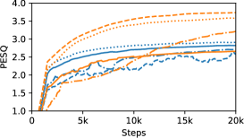
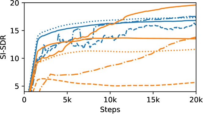
Figure 1: Performance in PESQ and SI-SDR over the training steps.

V Conclusion

This paper explored the distinctions among various diffusion-based frameworks for generative speech enhancement, explicitly focusing on score-based generative models and the SB. Through comprehensive experimental analysis, we highlighted the variations in training behaviors and performance across these frameworks. We introduced a novel perceptual loss function designed for the SB framework, significantly enhancing the performance and perceptual quality of the processed speech signals. To support ongoing research and innovation in this field, we made all experimental code and pre-trained models publicly accessible.

Future work could involve training the SB model on super-wideband speech, utilizing high-quality datasets such as EARS [35], and experimenting with various corruption types. Moreover, the impact of the EMA has not been investigated for generative speech enhancement.

References

- [1] J.-M. Lemercier, J. Richter, S. Welker, E. Moliner, V. Välimäki, and T. Gerkmann, “Diffusion models for audio restoration,” Signal Processing Magazin, accepted paper, 2025.
- [2] J. Richter, S. Welker, J.-M. Lemercier, B. Lay, T. Peer, and T. Gerkmann, “Causal diffusion models for generalized speech enhancement,” IEEE Open Journal of Signal Processing, 2024.
- [3] Y. Song, J. Sohl-Dickstein, D. P. Kingma, A. Kumar, S. Ermon, and B. Poole, “Score-based generative modeling through stochastic differential equations,” International Conference on Learning Representations, 2021.
- [4] T. Karras, M. Aittala, T. Aila, and S. Laine, “Elucidating the design space of diffusion-based generative models,” in Advances in Neural Information Processing Systems, 2022.
- [5] Y. Lipman, R. T. Q. Chen, H. Ben-Hamu, M. Nickel, and M. Le, “Flow matching for generative modeling,” in International Conference on Learning Representations, 2023.
- [6] T. Chen, G.-H. Liu, and E. Theodorou, “Likelihood training of Schrödinger bridge using forward-backward SDEs theory,” in International Conference on Learning Representations, 2021.
- [7] S. Welker, J. Richter, and T. Gerkmann, “Speech enhancement with score-based generative models in the complex STFT domain,” in ISCA Interspeech, 2022, pp. 2928–2932.
- [8] J. Richter, S. Welker, J.-M. Lemercier, B. Lay, and T. Gerkmann, “Speech enhancement and dereverberation with diffusion-based generative models,” IEEE/ACM Transactions on Audio, Speech, and Language Processing, vol. 31, pp. 2351–2364, 2023.
- [9] P. Gonzalez, Z.-H. Tan, J. Østergaard, J. Jensen, T. S. Alstrøm, and T. May, “Investigating the design space of diffusion models for speech enhancement,” arXiv preprint arXiv:2312.04370, 2023.
- [10] A. H. Liu, M. Le, A. Vyas, B. Shi, A. Tjandra, and W.-N. Hsu, “Generative pre-training for speech with flow matching,” in International Conference on Learning Representations, 2024.
- [11] A. Jukić, R. Korostik, J. Balam, and B. Ginsburg, “Schrödinger bridge for generative speech enhancement,” in ISCA Interspeech, 2024, pp. 1175–1179.
- [12] Z. Chen, G. He, K. Zheng, X. Tan, and J. Zhu, “Schrödinger bridges beat diffusion models on text-to-speech synthesis,” arXiv preprint arXiv:2312.03491, 2023.
- [13] D. P. Kingma and R. Gao, “Understanding diffusion objectives as the ELBO with simple data augmentation,” in Conference on Neural Information Processing Systems, 2023.
- [14] D. de Oliveira, S. Welker, J. Richter, and T. Gerkmann, “The PESQetarian: On the relevance of Goodhart’s law for speech enhancement,” in ISCA Interspeech, 2024, pp. 3854–3858.
- [15] J. Kim, M. El-Khamy, and J. Lee, “End-to-end multi-task denoising for joint SDR and PESQ optimization,” arXiv preprint arXiv:1901.09146, 2019.
- [16] C. Valentini-Botinhao, X. Wang, S. Takaki, and J. Yamagishi, “Investigating RNN-based speech enhancement methods for noise-robust text-to-speech,” ISCA Speech Synthesis Workshop, pp. 146–152, 2016.
- [17] S. Wang, S. Liu, A. Harper, P. Kendrick, M. Salzmann, and M. Cernak, “Diffusion-based speech enhancement with Schrödinger bridge and symmetric noise schedule,” arXiv preprint arXiv:2409.05116, 2024.
- [18] J.-M. Lemercier, J. Richter, S. Welker, and T. Gerkmann, “Storm: A diffusion-based stochastic regeneration model for speech enhancement and dereverberation,” IEEE/ACM Transactions on Audio, Speech, and Language Processing, vol. 31, pp. 2724–2737, 2023.
- [19] B. Lay, S. Welker, J. Richter, and T. Gerkmann, “Reducing the prior mismatch of stochastic differential equations for diffusion-based speech enhancement,” in ISCA Interspeech, 2023, pp. 3809–3813.
- [20] J. Berner, L. Richter, and K. Ullrich, “An optimal control perspective on diffusion-based generative modeling,” Transactions on Machine Learning Research, 2024.
- [21] P. Vincent, “A connection between score matching and denoising autoencoders,” Neural Computation, vol. 23, no. 7, pp. 1661–1674, 2011.
- [22] E. Schrödinger, “Sur la théorie relativiste de l’électron et l’interprétation de la mécanique quantique,” in Annales de l’institut Henri Poincaré, vol. 2, no. 4, 1932, pp. 269–310.
- [23] L. Richter and J. Berner, “Improved sampling via learned diffusions,” in International Conference on Learning Representations, 2024.
- [24] E. Nelson, Dynamical Theories of Brownian Motion. Princeton University Press, 1967, vol. 3.
- [25] C. Bunne, Y.-P. Hsieh, M. Cuturi, and A. Krause, “The Schrödinger bridge between gaussian measures has a closed form,” in International Conference on Artificial Intelligence and Statistics. PMLR, 2023, pp. 5802–5833.
- [26] Y. Luo and N. Mesgarani, “Conv-TasNet: Surpassing ideal time–frequency magnitude masking for speech separation,” IEEE Transactions on Audio, Speech, and Language Processing, vol. 27, no. 8, pp. 1256–1266, 2019.
- [27] S.-W. Fu, C. Yu, T.-A. Hsieh, P. Plantinga, M. Ravanelli, X. Lu, and Y. Tsao, “MetricGAN+: An improved version of MetricGAN for speech enhancement,” in ISCA Interspeech, 2021, pp. 201–205.
- [28] R. Chao, W.-H. Cheng, M. La Quatra, S. M. Siniscalchi, C.-H. H. Yang, S.-W. Fu, and Y. Tsao, “An investigation of incorporating Mamba for speech enhancement,” IEEE Spoken Language Technology Workshop, 2024.
- [29] T. Karras, M. Aittala, J. Lehtinen, J. Hellsten, T. Aila, and S. Laine, “Analyzing and improving the training dynamics of diffusion models,” in Proceedings of the IEEE/CVF Conference on Computer Vision and Pattern Recognition, 2024, pp. 24 174–24 184.
- [30] ITU-T Rec. P.863, “Perceptual objective listening quality prediction,” Int. Telecom. Union (ITU), 2018. [Online]. Available: https://www.itu.int/rec/T-REC-P.863-201803-I/en
- [31] A. Rix, J. Beerends, M. Hollier, and A. Hekstra, “Perceptual evaluation of speech quality (PESQ) - a new method for speech quality assessment of telephone networks and codecs,” in IEEE International Conference on Acoustics, Speech and Signal Processing, 2001, pp. 749–752.
- [32] J. Jensen and C. H. Taal, “An algorithm for predicting the intelligibility of speech masked by modulated noise maskers,” IEEE/ACM Transactions on Audio, Speech, and Language Processing, vol. 24, no. 11, pp. 2009–2022, 2016.
- [33] J. Le Roux, S. Wisdom, H. Erdogan, and J. R. Hershey, “SDR–half-baked or well done?” in IEEE International Conference on Acoustics, Speech and Signal Processing, 2019, pp. 626–630.
- [34] C. K. Reddy, V. Gopal, and R. Cutler, “DNSMOS: A non-intrusive perceptual objective speech quality metric to evaluate noise suppressors,” IEEE International Conference on Acoustics, Speech and Signal Processing, pp. 6493–6497, 2021.
- [35] J. Richter, Y.-C. Wu, S. Krenn, S. Welker, B. Lay, S. Watanabe, A. Richard, and T. Gerkmann, “EARS: An anechoic fullband speech dataset benchmarked for speech enhancement and dereverberation,” in ISCA Interspeech, 2024.