A Flexible Framework for Universal Computational Aberration Correction via Automatic Lens Library Generation and Domain Adaptation

Emerging universal Computational Aberration Correction (CAC) paradigms provide an inspiring solution to light-weight and high-quality imaging without repeated data preparation and model training to accommodate new lens designs. However, the training databases in these approaches, i.e., the lens libraries (LensLibs), suffer from their limited coverage of real-world aberration behaviors. Moreover, it is challenging to train a universal model for reliable results in a zero-shot manner, whose inflexible tuning pipeline is also confined to the lens-descriptions-known case. In this work, we set up an OmniLens framework for universal CAC, considering both the generalization ability and flexibility. OmniLens extends the idea of universal CAC to a broader concept, where a base model is trained as the pre-trained model for three cases, including zero-shot CAC with the pre-trained model, few-shot CAC with a little lens-specific data for fine-tuning, and domain adaptive CAC using domain adaptation for lens-descriptions-unknown lens. In terms of OmniLens’s data foundation, we first propose an Evolution-based Automatic Optical Design (EAOD) pipeline to construct the LensLib automatically, coined AODLib, whose diversity is enriched by an evolution framework, with comprehensive constraints and a hybrid optimization strategy for achieving realistic aberration behaviors. For network design, we introduce the guidance of high-quality codebook priors to facilitate both zero-shot CAC and few-shot CAC, which enhances the model’s generalization ability, while also boosting its convergence in a few-shot case. Furthermore, based on the statistical observation of dark channel priors in optical degradation, we design an unsupervised regularization term to adapt the base model to the target descriptions-unknown lens using its aberration images without ground truth. We validate the proposed OmniLens framework on $4$ manually designed low-end lenses with various structures and aberration behaviors. Remarkably, the base model trained on AODLib exhibits strong generalization capabilities, achieving $97\%$ of the lens-specific performance in a zero-shot setting. Extensive experiments also demonstrate that OmniLens outperforms the lens-specific method with only $5\%$ of data and training time, and the domain adaptation provides an effective solution to the cases with unknown lens descriptions. Our work holds the promise of becoming a seminal baseline for the field, which also delivers a powerful pre-trained foundation.

1 Introduction

Computational Aberration Correction (CAC), equipped with a post image restoration method to deal with the degradation (i.e., the optical degradation [1]) induced by residual optical aberrations of the target optical lens, is a fundamental and long-standing task [2, 3] in Computational Imaging. This technology is particularly highly demanded in mobile and wearable vision terminals for lightweight and high-quality photography [4, 5], where low-end lenses [6, 7] with simple structure and severe optical degradation are applied. Recent advances in CAC have centered around Deep Learning (DL) based methods [8, 9, 10]. Benefiting from the strong image restoration networks [11, 12, 13], DL-based CAC models can restore clear images for the target lens after being trained on the corresponding data pairs under lens-specific optical degradation [9, 1]. However, these trained CAC models have invariably been tailored to a specific lens, revealing limited generalization ability to other lens designs, or even different manufactured samples with tolerances [14]. Considering the variability of optical degradation across diverse lenses, the complex and time-consuming pipeline of lens analysis, imaging simulation, data preparation, and model training requires to be re-conducted for every new lens, limiting the applications of lens-specific CAC methods.

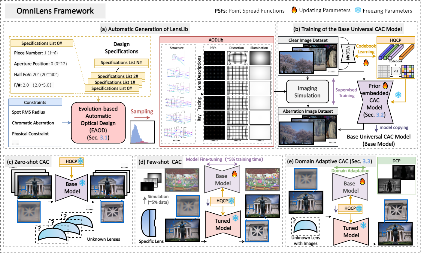
Figure 1: Overview of the established OmniLens framework. (a) The generation of AODLib with evolution-based automatic optical design. (b) Training pipeline for the base universal prior-embedded CAC model. The training data pairs are generated by imaging simulation building upon the lens descriptions of lens samples in AODLib. The pre-trained base universal model is applied to address three situations in universal CAC: (c) Zero-shot CAC, (d) Few-shot CAC, and (e) DA-CAC, where whether the description of the target lens is known or unknown is considered.

Consequently, developing a universal CAC model [15] to process the optical degradation of any imaging lens system has hit the forefront, which is a tremendously valuable yet formidable task in the field of DL-based CAC. In this article, we intend to set up a comprehensive solution to it, named OmniLens, whose overview is shown in Fig 1.

For the DL-based CAC model trained on paired aberration data, the performance depends heavily on whether the aberration distributions in the training database can cover those of the target lens. The key challenge lies in constructing a lens library (LensLib) containing diverse aberration distributions. Recent approaches for LensLib construction are mainly based on commercial lens databases (e.g., ZEBASE) [16, 15], i.e., ZEBASELib, or random Zernike model [17, 18], i.e., ZernikeLib. However, the former suffers from the limited number and coverage of lens samples, and the latter overlooks the domain shift of aberration distributions between generated virtual lenses and real-world ones.

As shown in Fig 1 (a), we first propose a novel LensLib construction method that addresses these limitations, which builds upon an Evolution-based Automatic Optical Design (EAOD) pipeline, centering around an evolution framework [19] with both global and local optimization mechanisms [20, 21] incorporated. Starting from multiple sets of random initial points of lens parameters, EAOD is designed to search for multiple solutions under given specifications through hybrid global and local optimization, where these solutions are mutated by evolution strategy as the initial points of the next search turn for more possible structures. Additionally, both optimization processes are constrained by a combination of imaging quality and physical constraints, to achieve machinable and practical solutions with the image quality reaching the upper limit of the current structure. Benefiting from the above designs, EAOD can automatically generate a large number of lens samples that closely resemble real-world lenses, ensuring the reasonable and real aberration distributions of the LensLib. We use EAOD to generate about $12,000$ lens samples with different specifications (e.g., piece number, aperture position, half FoV, and F-number), which are sampled based on their average RMS spot radii to construct the LensLib with required aberration distributions. AODLib is constructed to serve as the data fundamental for OmniLens, based on which we train a base universal CAC model as the pre-trained model in this field, as shown in Fig. 1 (b).

Aside from the construction of LensLib, yielding robust performance under all possible optical degradation in a zero-shot manner is a prominent challenge for universal CAC, as the target lens always appears as a new, previously unseen sample to the training base. A compromise is to fine-tune the pre-trained universal model with the lens-specific data [16] for comparable performance to the lens-specific model within a much shorter training time. Yet, this solution still calls for known lens descriptions to prepare large amounts of lens-specific data, whose overall training pipeline remains time-consuming and is unsuitable for unknown lenses. Recently, Domain Adaptation (DA) [22, 23, 24] delivers remarkable performance on cross-domain image restoration tasks, which is a powerful pipeline for transferring the model to a shifted data domain without the ground-truth but has not been explored in tuning the universal CAC model.

To this intent, we look into the issue of tuning a CAC model for an unknown lens from a novel perspective of DA, where the base model is adapted to the description-unknown lens without access to the paired data. Integrating the DA pipeline with the pre-trained base model, the OmniLens framework extends the universal CAC into three situations, including zero-shot CAC with a universal model (ZS-CAC), few-shot CAC (FS-CAC) with a little lens-specific data for fine-tuning, and the domain adaptive CAC (DA-CAC) with little unpaired target domain data. In terms of the model design, we introduce the Prior-embedded CAC Model (PCM) where the pre-trained High-Quality Codebook Priors (HQCP) [25, 26] are embedded into the network by serving as an additional modality. Guiding the CAC process with quantized pre-learned high-quality details, HQCP effectively enhances the model’s generalization ability, while also boosting the convergence of the model under the challenging few-shot setting. Moreover, we develop an efficient framework for conducting domain adaptation on the CAC model based on the statistic Dark Channel Prior (DCP) [27] of optical degradation. Inspired by the observation [27] that DCP often exists in convolution-induced blur, we experimentally verify that optical degradation exhibits DCP, where the number of non-zero pixels in the dark channel images under optical degradation is significantly larger than those without aberrations. In this way, DCP serves as an unsupervised regularization term to constrain the CAC model during domain adaptation.

Four types of lenses with diverse severity and behaviors of aberrations are employed to validate OmniLens’s effectiveness. Experimental results in all testing cases demonstrate that OmniLens provides a robust and flexible solution to the universal CAC from the following aspects: i) AODLib greatly enhances the generalization of the trained universal CAC model compared to ZernikeLib and ZEBASELib; ii) Through FS-CAC, OmniLens achieves superior results to the lens-specific model with only $5\%$ of training data and training time, where the HQCP contributes to fast convergence of the model; iii) Without access to the ground truth, the DCP-based domain adaptation pipeline brings significant improvements to the base universal model, especially when the model fails in ZS-CAC. Last but not least, trained under AODLib, the universal model in OmniLens can serve as a powerful pretraining model for the CAC field, contributing to raising the upper limit of lens-specific CAC.

2 Problem Formulation

In this article, we investigate the DL-based CAC pipeline, where an image restoration network (coined CAC model) pre-trained on the aberration-clear data pairs is utilized for restoring images under optical aberration captured by the target low-end lens [9, 15].

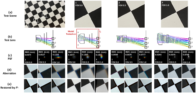
Figure 2: Illustration of failure cases of the lens-specific model. (a): The test scene of checkerboard. The normalized FoVs of $0.0$, $0.5$, and $1.0$ are focused. (b)$\sim$(d): The distinct aberration behavior for different structures of lenses. (d): We train a lens-specific model $F^{L_{j}}$ on the data of the second lens (taken as $L_{j}$) with the most severe optical degradation, which is applied to restore aberration images of all the test lenses. The lens-specific model delivers almost no generalization ability, introducing artifacts when dealing with optical degradation under other aberration behaviors.

2.1 Lens-Specific CAC

Aberration behaviors vary dramatically with the lens structure, making each possible low-end lens suffer unique optical degradation, as shown in Fig. 2 (b)$\sim$(d). To tackle such degradation, lens-specific CAC pipeline is often applied [1, 9, 28], where the synthetic data pairs $\mathcal{D}^{L_{j}}_{S}{=}\{{y^{L_{j}}_{S}}^{(i)},{x}^{(i)}\}_{i=1}^{N}$ are generated by imaging simulation model based on the lens descriptions of the target-specific lens $L_{j}$. In this case, trained on $\mathcal{D}^{L_{j}}_{S}$, the lens-specific CAC model $F^{L_{j}}$ can only deal with target aberration images $y^{L_{j}}_{T}$ captured by $L_{j}$, which tends to fail when faced with aberration images from other lenses $L_{k,l,n,\cdots}$, as shown in Fig. 2 (e). Note that the $j,k,l,n,\cdots$ represent the labels for different target lenses. Consequently, for the sake of the effectiveness of CAC, for almost every lens, lens-specific CAC requires re-conducting the data generation and model training pipeline, which is time-consuming and inflexible.

2.2 Universal CAC

As illustrated in Fig. 1 (c), universal CAC targets at training a universal model $F$ to restore aberration images $y^{L_{j,k,l,n,\cdots}}_{T}$ from any unknown lens $L_{j,k,l,n,\cdots}$ in a zero-shot manner. This solution is achieved by training the model on a large database $\mathcal{D}_{S}{=}\{{y_{S}}^{(i)},{x}^{(i)}\}_{i=1}^{N}$ covering aberration images under as diverse as possible optical degradation [15]. However, $\mathcal{D}_{S}$ can hardly cover all possible aberration behaviors of $L_{j,k,l,n,\cdots}$, while it is also formidable for $F$ to handle multiple optical degradations via supervised learning, leading to the sub-optimal results of ZS-CAC.

This article extends the idea of universal CAC to a broader concept, i.e., the above universal CAC model serves as a pre-trained base model $F^{B}$. On this basis, fast and flexible fine-tuning strategies are explored to adapt it to the target-specific lens. In terms of the descriptions-known specific lens, as shown in Fig. 1 (d), taking $L_{j}$ for example, we only generate about $5\%$ synthetic data pairs $\mathcal{D}^{L_{j}}_{S}{=}\{{y^{L_{j}}_{S}}^{(i)},{x}^{(i)}\}_{i=1}^{M}$ ($M\approx 5\%*N$) for fine-tuning the $F^{B}$ within $5\%$ training time of the lens-specific CAC in a few-shot manner. Meanwhile, Fig. 1 (e) shows the domain-adaptive CAC pipeline for fine-tuning $F^{B}$ with un-paired images $\mathcal{D}^{L_{k}}_{T}{=}\{{y^{L_{k}}_{T}}^{(i)}\}_{i=1}^{K}$ taken by the descriptions-unknown specific lens ($L_{k}$ for example) via domain adaptation strategy. Similarly, the training time for DA-CAC is kept at about $5\%$ of the lens-specific CAC to ensure a flexible pipeline.

3 Method

In this section, a flexible framework OmniLens is introduced as the solution to the above extended universal CAC task. We first propose a novel pipeline of generating a large number of lens samples under diverse and realistic aberration behaviors automatically in Sec. 3.1, to build up an extensive lens database $\mathcal{D}_{S}$, which is the key to training an effective universal CAC model. Then, a High-Quality Codebook Prior (HQCP) is employed to facilitate the fast and flexible fine-tuning of the CAC model in Sec. 3.2. In addition, in Sec. 3.3, we further develop a domain adaptation framework based on the statistic Dark Channel Prior (DCP) of the optical degradation, enabling efficient model tuning with the ground-truth-free data of the target lens.

3.1 Generation of LensLib with Automatic Optical Design

In universal CAC, a lens library (LensLib) $\mathrm{L}_{lib}{=}\{{L_{j},L_{k},L_{l},\cdots}\}$ covering diverse and realistic aberration behaviors is significant for training a robust model to handle optical degradation of unknown lenses. However, as aforementioned, the aberration behavior between different lens structures varies greatly, which requires a large scale of samples to traverse. Considering the highly free, empirical, and hard-to-reproduce process of optical design, constructing a LensLib via designing a large number of diverse lens structures manually is challenging. To tackle this dilemma, in OmniLens, we pioneer to generate the LensLib by automatic optical design, where an Evolution-based Automatic Optical Design (EAOD) method is proposed to produce diverse optimized lens samples with design specifications and constraints fed in batch.

3.1.1 Modeling the Automatic Optical Design

To increase the diversity in aberration behaviors for automatically designed lenses, four types of specifications that deliver large impacts on the final aberration behavior, i.e., the piece number $S_{p}$, aperture position $S_{aper}$, half FoV $S_{FoV}$ and F number $S_{F}$ of the lens, are considered. Meanwhile, we characterize a lens structure by its curvatures, glass, and air spacings, refractive indexes, and Abbe numbers, defining a normalized lens parameters vector, whose dimension and value range meet the given specifications $\mathcal{S}^{(j)}{=}\{S_{p}^{(j)},S_{aper}^{(j)},S_{FoV}^{(j)},S_{F}^{(j)}\}$:

$$P^{\mathcal{S}^{(j)}}=(p^{(1)},p^{(2)},...,p^{(n)})^{T}\in\mathbb{R}^{n}.$$ (1)

The objective of the automatic design is to find the optimal $P^{\mathcal{S}^{(j)}}$ to minimize the loss function $\mathcal{L}_{EAOD}(P^{\mathcal{S}^{(j)}})$. Several constraints are taken into account, including imaging quality constraints and physical structure constraints, which compose the $\mathcal{L}_{EAOD}$ to ensure that the output structure is a realizable case in practical applications. Specifically, we quantify the average spot RMS radius across all sampled FoVs and wavelengths into $\mathcal{L}_{spt}$, and average lateral chromatic aberration into $\mathcal{L}_{c}$, whose weighted sum constitutes the imaging quality loss $\mathcal{L}_{IQ}$:

$$\mathcal{L}_{IQ}=\mathcal{L}_{spt}+\lambda_{c}\mathcal{L}_{c}.$$ (2)

Moreover, key physical properties of the lens, e.g., total track length, effective focal length, and edge spacing between two adjacent surfaces, derived from $P^{\mathcal{S}^{(j)}}$, are constrained by a linear penalty function to fall within a reasonable range:

$$\mathcal{L}_{P}=\dfrac{1}{n_{P}}\sum^{n_{P}}_{i=1}\alpha_{i}[\max(q^{(i)}_{min}-q_{i},0)+\max(q_{i}-q^{(i)}_{max},0)],$$ (3)

where $n_{P}$ physical quantities $q_{i}$ are constrained between $q^{(i)}_{min}$ and $q^{(i)}_{max}$, and the constraint ratio is regulated by weight $\alpha_{i}$. We employ $\mathcal{L}_{P}$ to ensure machinable output structures while meeting the specifications, in particular preventing adjacent surfaces from being too close together or even overlapped, which is a common error in the optical design process. The overall loss function $\mathcal{L}_{EAOD}$ considering both imaging quality and physical constraints with a balancing weight $\lambda_{P}$ is expressed as:

$$\mathcal{L}_{EAOD}=\mathcal{L}_{IQ}+\lambda_{P}\mathcal{L}_{P}.$$ (4)

Please refer to the supplemental document for more details about the implementation of $\mathcal{L}_{EAOD}$. Finally, EAOD aims to seek as many lens structures as possible under $\mathcal{S}^{(j)}$, and generate lens samples with their imaging quality optimized to the upper limit of the corresponding structure, which is modeled as:

$$\mathrm{L}^{\mathcal{S}^{(j)}}=M_{EAOD}(\mathcal{S}^{(j)}),$$ (5)

where $\mathrm{L}^{\mathcal{S}^{(j)}}{=}\{{L^{\mathcal{S}^{(j)}}}^{(i)}\}_{i=1}^{N}$ denotes the generated lens samples under $\mathcal{S}^{(j)}$, and $M_{EAOD}$ is the EAOD method. With the lens samples produced in all set specifications $\mathcal{S}{=}\{\mathcal{S}^{(j)}\}_{j=1}^{M}$, we can construct the LensLib $\mathrm{L}_{lib}{=}\{{\mathrm{L}^{\mathcal{S}^{(j)}}}\}_{j=1}^{M}$.

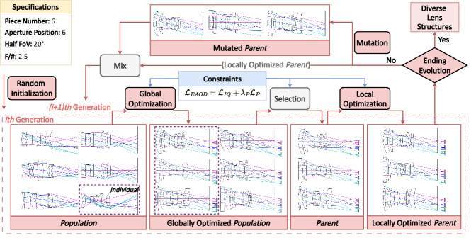
Figure 3: Overall pipeline of the proposed EAOD method. Taking the lens specifications of $6$ piece as an example, the EAOD leverages a hybrid global and local optimization strategy to seek diverse lens structures that maximally satisfy both imaging quality and physical constraints from generation to generation based on an evolution framework with mutation mechanism.

3.1.2 Pipeline for Evolution-based Automatic Optical Design

The overall pipeline of the proposed EAOD method is shown in Fig. 3. The core idea for EAOD lies in a Genetic Algorithm (GA) based evolution framework to produce diverse optimized lens structures from generation to generation via iteration. In this way, more possible high-quality lens structures can be achieved under one given set of specifications.

First and foremost, we define a $Population$ composed of all lens structures to be optimized, where each structure is coined an $Individual$. Without any empirical preference, the $Individual$ is the normalized lens parameters vector $P^{\mathcal{S}^{(j)}}$ from random initialization, and $m$ $Individuals$ constitute the $Population$:

$$\mathrm{P}^{\mathcal{S}^{(j)}}=\{P^{\mathcal{S}^{(j)}}_{1},P^{\mathcal{S}^{(j)}}_{2},...,P^{\mathcal{S}^{(j)}}_{m}\}.$$ (6)

Then, a hybrid global and local optimization strategy is proposed to find multiple promising high-quality structures $\hat{\mathrm{P}}^{\mathcal{S}^{(j)}}$ for $\mathrm{P}^{\mathcal{S}^{(j)}}$, coined the $Parent$, which minimizes the $\mathcal{L}_{EAOD}$. Concretely, the global optimization method, e.g., Simulated Annealing Algorithm (SAA) [29] or Particle Swarm Optimization (PSO) [30], is employed to rapidly drive the randomly initialized $Individuals$ towards the location of the global optimal solution, where the solutions with superior $\mathcal{L}_{EAOD}$ are selected for the following local optimization; while the local optimization method, e.g., ADAM [31] or Damped Least Squares (DLS) [32], aims to seek their local optima for the relatively best imaging results under the primarily optimized structures. In addition, we employ the mutation mechanism in GA on $Parent$ to generate more possible structures, where for each $Individual$ ${\hat{{P}}^{\mathcal{S}^{(j)}}}_{i}$ in $Parent$, $\gamma$ percentage of its parameters are randomly selected for random initialization. The mutated $Parent$ is then mixed with the origin $Parent$ to serve as the start points of the next generation. Finally, the hybrid optimization, selection, and mutation processes are re-conducted for each generation, where the $Parent$ is outputted as the diverse lens structures when the generation meets the set number.

In general, EAOD uses the evolution mechanism to satisfy the needs of the diversity in the lens structures for constructing the LensLib, while applying the hybrid optimization to ensure the best imaging quality for the current structure, which drives the aberration distributions of the generated samples more close to those of real-world ones.

3.1.3 Sampling Strategy for LensLib Construction

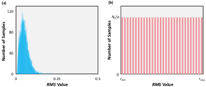
Figure 4: Illustration of our sampling strategy. (a): The $RMS$ distribution of initial LensLib $\mathrm{L}_{lib}$. (b): The ideal $RMS$ distribution of the final AODLib ${\mathrm{L}}_{AODLib}$.

With all sets of specifications $\mathcal{S}$ fed into EAOD as in Eq. 5, the initial LensLib $\mathrm{L}_{lib}$ is constructed. However, without any explicit design in EAOD to deliver reasonable distribution for aberration behaviors of the generated lens samples, it is still difficult to train a general CAC model with strong generalization ability on such a LensLib. We use the average RMS spot radii (${\mu}{m}$) across all FoVs and wavelengths ($RMS$ for short) of a lens to quantize its aberration behavior, which can intuitively reflect the severity of its aberrations, drawing the $RMS$ distribution histogram, i.e., the aberration distribution, of $\mathrm{L}_{lib}$ in Fig. 4 (a). It can be observed that the $RMS$ of most samples in $\mathrm{L}_{lib}$ is concentrated in the middle range, which means that the samples of severe or mild aberrations are relatively scarce, unconsciously introducing data preference issues.

To overcome this issue, we propose a sampling strategy to sample a portion of lenses from the $\mathrm{L}_{lib}$ to construct the final AODLib ${\mathrm{L}}_{AODLib}$ with a relatively reasonable $RMS$ distribution under a given sampling number $N_{S}$:

$$\mathrm{L}_{AODLib}{=}\{L^{(s)}\}_{s=1}^{N_{S}}=Sampling(\mathrm{L}_{lib},r_{min},r_{max},N_{S}).$$ (7)

Ideally, as shown in Fig. 4 (b), we hope to obtain a uniform distribution of the $RMS$ within the range $[r_{min},r_{max}]$ for the ${\mathrm{L}}_{AODLib}$, mitigating the data preference towards any certain level of aberration, where $[r_{min},r_{max}]$ determines ${\mathrm{L}}_{AODLib}$’s coverage scope of aberration levels. Specifically, $[r_{min},r_{max}]$ is divided into $a$ sub-intervals, and $N_{S}/a$ samples are randomly sampled from each of them, to achieve a relative uniform distribution across these sub-intervals. The optimal $r_{min}$, $r_{max}$, $N_{S}$, and sampling distribution will be experimentally investigated in Sec. 5.4.

With the sampled ${\mathrm{L}}_{AODLib}$, a universal CAC dataset $\mathcal{D}_{S}{=}\{{y_{S}}^{(i)},{x}^{(i)}\}_{i=1}^{N}$ of aberration-clear image pairs under diverse optical degradation can be prepared via imaging simulation. We employ a ray-tracing model [1] to calculate the lens descriptions, i.e., the PSFs, distortion, and illumination maps, for all samples in ${\mathrm{L}}_{AODLib}$, which are applied to simulate aberration images via patch-wise convolution and distortion transformation. The data preparation process will be depicted in Sec. 4.

3.2 Universal CAC Model with High-Quality Codebook Priors

A universal CAC model $F^{B}$ can be trained on $\mathcal{D}_{S}$ via supervised learning, which can also serve as a pre-trained base model for training a more powerful lens-specific CAC model via few-shot fine-tuning. Nevertheless, the CAC task is an ill-posed problem, where the details of the high-quality image corrupted by optical degradation are hard to retrieve. Without any useful image prior, the universal CAC model can hardly learn such a many-to-one mapping and suffers the risk of over-fitting to the training dataset $\mathcal{D}_{S}$.

Inspired by the pioneering works on image generation models [33, 34], we develop a Prior-embedded CAC Model (PCM) that introduces High-Quality Codebook Priors (HQCP) to mitigate the issue, as shown in Fig. 5. The core idea of PCM is to learn the distribution of clear, high-quality images, which are quantized to guide the CAC process. We implement this process using the Vector-Quantized (VQ) codebook learning in VQGAN [35, 36], which requires a smaller training scale compared to diffusion models [37] without introducing significant additional computational overhead during inference. Our PCM starts from a baseline FeMaSR model [26], where we elevate it into a more effective and general model paradigm.

In the VQGAN pre-training stage, the clear images are encoded into a discrete latent space to learn a codebook characterizing the high-quality image features. During the CAC process, encoded deep features of an aberration image are progressively mapped into such a latent space with an enhancement module of convolution or Transformer blocks in low-level vision [38, 11, 13, 39], i.e., the Residual Swin-Transformer Block (RSTB) [11] in our case. Then, the enhanced features, denoted by $\hat{f}$, serve two purposes: (i) reconstructing the high-quality clear image by an HQCP-guided decoder group $Dec$, and (ii) generating HQCP via feature matching with the codebook to guide the reconstruction process. Specifically, for $\hat{f}$ with spatial size $(h\times{w})$ and channel dimension $n$, we find the nearest neighbours in the learned codebook $\mathcal{Z}=\{z_{k}\}_{k=1}^{K}\in\mathbb{R}^{n}$ for its each element $\hat{f}_{ij}$, to obtain the quantized features $\hat{f}^{q}\in\mathbb{R}^{h{\times}w{\times}n}$:

$$\hat{f}^{q}_{ij}=\arg\min\limits_{z_{k}\in\mathcal{Z}}(\|{\hat{f}_{ij}-z_{k}}\|_{2}),$$ (8)

where $K$ denotes the codebook size and $i\in\{1,2,\cdots,h\}$, $j\in\{1,2,\cdots,w\}$ denote the coordinates in the feature space. Furthermore, the pre-trained decoder group $Dec_{vq}$ in VQGAN is employed to produce HQCP features from $\hat{f}^{q}$, which are used to guide the reconstruction features in $Dec$ through a fusion module $Fusion$:

$$\hat{f}^{\prime}_{i+1}=Dec(Fusion(\hat{f}^{\prime}_{i},\hat{f}^{\prime q}_{i}),i+1),\hat{f}^{\prime q}_{i}=Dec_{vq}(\hat{f}^{\prime q}_{i-1},i)$$ (9)

where the features $\hat{f}^{\prime}_{i}$ and $\hat{f}^{\prime q}_{i}$ from the $i$th layer of $Dec$ and $Dec_{vq}$ are fused by $Fusion$, and then fed to the $(i+1)$th layer of $Dec$ to produce reconstructed features $\hat{f}^{\prime}_{i+1}$. In PCM, we take the HQCP features as an additional modality, so that the fusion module can be any common multi-modal fusion method, e.g., add, concatenation (Concat.), Deformable Convolution Network (DCN) [40], Multi-modal Cross Attention (MCA) [41], and Spatial Feature Transformation (SFT) [42]. In our case, we adopt SFT for its superior performance. Referring to FeMaSR [26], the training objective $\mathcal{L}_{PCM}$ for PCM is a combination of L1, perceptual, adversarial, and codebook losses for generating visual-pleasant and realistic CAC results, which is applied in both ZS-CAC and FS-CAC.

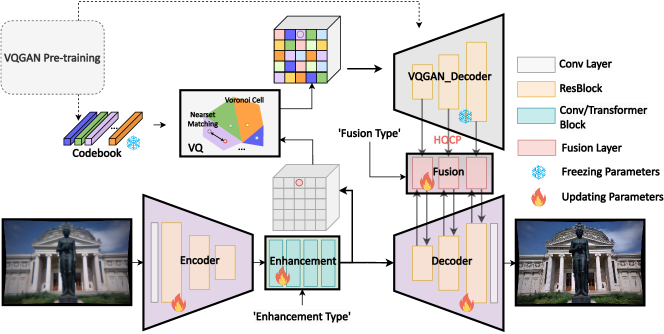
Figure 5: Overview of the Prior-embedded CAC Model (PCM). In our case, we employ RSTB as the ‘Enhancement Type’ and SFT as the ‘Fusion Type’. A VQGAN is pre-trained via self-supervised VQ codebook learning [36] to learn and characterize the HQCP for guiding the CAC process. The pre-trained VQGAN including the codebook is frozen during the CAC stage, where the parameters of the encoder, enhancement module, fusion module, and decoder are updated.

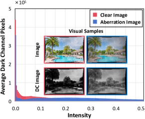
Figure 6: Illustration of dark channel prior in CAC. We draw the intensity (i.e., normalized grayscale) histogram of the DC images for aberration-clear image pairs based on DIV2K [43]. Combining the visual samples, the optical degradation reveals the property of DCP, where the aberration images have far fewer dark channel zero pixels than clear ones.

3.3 Domain Adaptation with Dark Channel Prior

To address the issues of unavailable lens-specific data pairs and the failure of ZS-CAC in scenarios with unknown lens descriptions, we propose an efficient DA-CAC framework, where only few aberration images captured $\mathcal{D}^{L_{k}}_{T}{=}\{{y^{L_{k}}_{T}}^{(i)}\}_{i=1}^{K}$ by the target lens $L_{k}$ are required to adapt the base model $F^{B}()$ trained on $D_{S}$ (the source domain) to $\mathcal{D}^{L_{k}}_{T}$’s optical degradation domain (the target domain).

In the field of domain adaptation for low-level vision, effective frameworks [44, 45, 46] are often built upon the statistical priors of degraded images or clean images, e.g., the Dark Channel Prior (DCP) [47] in image dehazing, which provides a direct unsupervised regularization for model training. Motivated by the observation from [27] that convolution-induced blur often exhibits DCP, optical degradation is also likely to possess DCP as it is evidently a form of such blur. To this end, we use the DIV2K dataset of natural images, and without loss of generality, choose the second lens in Fig. 2 to construct aberration-clear image pairs. The Dark Channel (DC) image $D(I)$ for an image $I$ can be calculated via a minimum value filtering operation:

$$D(I)=\min\limits_{y\in\mathcal{N}(x)}(\min\limits_{c\in\{r,g,b\}}I^{c}(y)),$$ (10)

where $I^{c}$ is the $c$th color channel, $x,y$ are pixel locations, and $\mathcal{N}(x)$ represents an image patch centered at $x$. We statistically analyze the intensity distribution histograms of the $D(I)$ for all the aforementioned aberration-clear image pairs as shown in Fig. 6, where a set of visual samples of $I$ and $D(I)$ is also provided. Corroborating our hypothesis, the elements in DC images for clear natural images mostly tend towards zero, while aberration images exhibit far more non-zero pixels in their DC images, indicating that optical degradation indeed possesses DCP.

Based on the observation, we propose to utilize the DCP loss function $\mathcal{L}_{DCP}$ as an unsupervised constraint on the restored aberration images ${y^{\prime L_{k}}_{T}}^{(i)}$ of the target lens $L_{k}$:

$${y^{\prime L_{k}}_{T}}^{(i)}=F^{B}({y^{L_{k}}_{T}}^{(i)}),$$ (11)

$$\mathcal{L}_{DCP}=\|{D({y^{\prime L_{k}}_{T}}^{(i)})}\|_{1},$$ (12)

where the $D({y^{\prime L_{k}}_{T}}^{(i)})$ will be pulled towards zero to align with the dark channel distribution of natural clear images. To improve the stability of the DA training, we also adopt the $\mathcal{L}_{PCM}$ to provide supervision on the source domain AODLib data $\mathcal{D}_{S}$, constructing the overall training objective $\mathcal{L}_{DA}$ for the DA-CAC framework:

$$\mathcal{L}_{DA}=\lambda_{S}\mathcal{L}_{PCM}+\lambda_{T}\mathcal{L}_{DCP},$$ (13)

where $\lambda_{S}$ and $\lambda_{T}$ are weights to control the training stability.

4 Implementation Details

4.1 Data Preparation Process

We choose and reshape $2111$ natural images with a resolution of $1920{\times}1280$ from the Flickr2K dataset [43] as the ground-truth to generate training dataset $D_{S}$ based on the AODLib $\mathrm{L}_{AODLib}$. For each image, a lens sample is randomly selected from $\mathrm{L}_{AODLib}$, whose lens descriptions are fed into a comprehensive imaging simulation pipeline [1] with the image, considering the impacts of both the ISP and distortion. More details of the pipeline can be found in the supplemental document. In this way, we prepare a convincing training set $D_{S}$ for universal CAC.

As a competing solution, we also prepare training data for the lens-specific method. For each target lens $L_{j}$, a training set $\mathcal{D}^{L_{j}}_{S}$ is constructed on the same ground-truth images as $D_{S}$ to train a lens-specific model. Besides, for FS-CAC, we randomly select only $5\%$ images in Flickr2K for data preparation. Following the common practice [48, 14], the perturbation method is employed to address the potential synthetic-to-real gap issue in lens-specific method, where $5$ sets of perturbed lens parameters of $L_{j}$ within a ${\pm}5\%$ range are randomly selected to be fed into the aforementioned simulation pipeline.

In terms of the test set for evaluation, to avoid information leakage, the validation set of another natural images dataset DIV2K ($92$ images of $1920{\times}1280$) is utilized to generate the test image pairs for each target lens. Different from $\mathcal{D}^{L_{j}}_{S}$, for test images, we conduct once ${\pm}2.5\%$ range of perturbation on the lens parameters to simulate the gap between the real lenses and the simulated ones. Similarly, the un-paired training data $\mathcal{D}^{L_{j}}_{T}{=}\{{y^{L_{j}}_{T}}^{(i)}\}_{i=1}^{K}$ ($K{=}78$) for DA-CAC is prepared with $10\%$ of DIV2K’s training set, where the ground-truth is unavailable following the unsupervised training rule.

4.2 Evaluation Protocol

To evaluate the effectiveness of the proposed OmniLens framework in universal CAC, $4$ manually designed specific lenses with different levels and behaviors of aberrations (shown in Fig. 2 (b)${\sim}$(d)) are applied as the test samples. We call them Lens-1P-I, Lens-1P-II, Lens-2P, and Lens-3P according to their numbers of pieces. A synthetic benchmark for universal CAC, consisting of test sets under each test lens, is set up based on the above data preparation process, where the referenced numerical metrics can be calculated for evaluation. To provide a comprehensive evaluation, referencing the NTIRE2024-RAIM [49], we employ PSNR, SSIM [50], LPIPS [51], DISTS [52], and NIQE [53] as the evaluation metrics, which cover both fidelity-based and perceptual-based assessments. Based on them, an overall metric $Score$ in [49] is defined to offer an intuitive evaluation, serving as the ultimate criterion for assessing the performance of the CAC solutions:

$$\begin{split}&Score=20\times\frac{PSNR}{50}+15\times\frac{SSIM-0.5}{0.5}+20\times\frac{1-LPIPS}{0.4}\\ &+40\times\frac{1-DISTS}{0.3}+30\times\frac{1-NIQE}{10}.\end{split}$$ (14)

4.3 Construction of AODLib

The value ranges for design specifications are consistent with those shown in Fig. 1 (a), i.e., $1{\sim}6$ for piece number with an interval of $1$, $20^{\circ}{\sim}40^{\circ}$ for half FoV with an interval of $2^{\circ}$, and $2.0{\sim}5.0$ for F number with an interval of $0.3$. Notably, the aperture position is determined based on the piece number, which can be located before or after each piece for a given piece number. In terms of the evolution strategy in EAOD, the degree of mutation is set to $30$, and the number of generations is set to $20$, to ensure the diversity of the generated lens structures. To strike a fine trade-off between optimization capability and convergence speed, we apply SAA and ADAM for the global optimization and local optimization in EAOD respectively. In addition, $\mathcal{L}_{P}$ is used on effective focal length, distortion, edge spacing, glass edge thickness, back focal length, total track length, and image height, with $\alpha_{i}$ being $\{0.1,1,0.1,0.1,0.05,0.01,1\}$. The loss weights for $\mathcal{L}_{EAOD}$ are set as $\lambda_{c}{=}0.25$ and $\lambda_{P}{=}1$ empirically.

Based on the above settings, we generate about $12,000$ lens structures through EAOD, which are sampled by the sampling strategy. Specifically, the $N_{S}$, $r_{min}$, $r_{max}$, $a$ are set to $\{1000,0,2.0,2\}$ for sampling $1000$ samples with a uniform $RMS$ distribution over $[0,2.0]$, while ensuring that the number of samples falling within each sub-interval reaches $N_{S}/a$.

4.4 Model Training and Fine-Tuning

In all the training processes in OmniLens, the Adam optimizer [31] is utilized with $\beta_{1}{=}0.9$, $\beta_{2}{=}0.99$ to train the model with a batch size of $8$ on randomly cropped images of $256{\times}256$. The model training is implemented with PyTorch [54] and on two NVIDIA GeForce RTX 3090 GPUs.

Similar to [26], the codebook is trained via VQ codebook learning on Flickr2K with a codebook size of $K{=}1024$, and the dimension of $n{=}512$, for $200K$ iterations. With the pre-trained VQGAN frozen, we train the base universal CAC model via $L_{PCM}$ with a fixed learning rate of $2e{-}4$ for $200K$ iterations. During the fine-tuning stage for FS-CAC, the learning rate is set to $2e{-}5$, where the model is only trained for $10K$ iterations based on the pre-trained base model. While for DA-CAC, we fine-tune the pre-trained base model with the DA objective $L_{DA}$, where $\lambda_{S}$ and $\lambda_{T}$ are set to $0.01$ and $1$ respectively. The DA training takes $5K$ iterations with a learning rate of $2e{-}6$. Additionally, for the lens-specific solution, a CAC model needs to be trained from scratch for each test lens with a learning rate of $2e{-}4$ and $200K$ iterations.

5 Experiments and Results

5.1 Comprehensive Results of OmniLens

We first compare our OmniLens framework with the traditional lens-specific CAC solution, which requires re-conducting the data preparation and model training pipelines for each test lens, serving as the theoretical upper limit for a universal CAC solution.

Table 1: Quantitative evaluation of OmniLens. For conciseness, we only list the representative results under PSNR, SSIM, LPIPS, and the overall $Score$. The detailed results for all metrics can be found in the supplemental document. In addition to the basic solutions, we include the results for Specific-FS and OmniLens-Full. Specific-FS means the lens-specific model trained on the few-shot setting, while OmniLens-Full is the full-trained lens-specific model initialized with the pre-trained OmniLens base model. We highlight the best and second best $Score$.

Test Lens

Lens-1P-I

Lens-1P-II

Lens-2P

Lens-3P

Average

PSNR$\uparrow$ / SSIM$\uparrow$ / LPIPS$\downarrow$

Score$\uparrow$

PSNR$\uparrow$ / SSIM$\uparrow$ / LPIPS$\downarrow$

Score$\uparrow$

PSNR$\uparrow$ / SSIM$\uparrow$ / LPIPS$\downarrow$

Score$\uparrow$

PSNR$\uparrow$ / SSIM$\uparrow$ / LPIPS$\downarrow$

Score$\uparrow$

PSNR$\uparrow$ / SSIM$\uparrow$ / LPIPS$\downarrow$

Score$\uparrow$

Specific-FS

26.876 / 0.811 / 0.1301

83.369

20.100 / 0.743 / 0.1736

73.730

26.239 / 0.819 / 0.1134

85.149

25.330 / 0.831 / 0.0916

89.397

24.636 / 0.801 / 0.1272

82.911

Specifc-Full

28.991 / 0.855 / 0.0748

93.560

20.124 / 0.780 / 0.1389

80.107

27.469 / 0.854 / 0.0937

90.018

27.742 / 0.878 / 0.0561

96.206

26.081 / 0.842 / 0.0909

89.973

OmniLens-ZS

26.908 / 0.827 / 0.1116

87.644

22.916 / 0.782 / 0.1651

73.981

27.935 / 0.869 / 0.0942

90.377

28.952 / 0.881 / 0.0639

95.345

26.678 / 0.840 / 0.1087

86.837

OmniLens-FS

28.921 / 0.841 / 0.0797

91.518

20.354 / 0.782 / 0.1285

79.288

29.061 / 0.867 / 0.0618

93.988

28.852 / 0.886 / 0.0559

95.942

26.797 / 0.844 / 0.0815

90.184

OmniLens-DA

27.456 / 0.836 / 0.1028

88.842

24.098 / 0.789 / 0.1606

74.973

28.762 / 0.874 / 0.0931

90.378

29.312 / 0.885 / 0.0607

95.445

27.407 / 0.846 / 0.1043

87.409

OmniLens-Full

29.318 / 0.853 / 0.0706

94.618

20.555 / 0.793 / 0.1229

82.066

28.873 / 0.875 / 0.0600

93.831

28.927 / 0.886 / 0.0535

96.809

26.918 / 0.852 / 0.0768

91.831

5.1.1 Evaluation on Synthetic Images

Tab. 1 presents the quantitative results under our evaluation protocol on the synthetic benchmark in 4, where the average results across the $4$ test lenses are calculated as the overall assessment for each method. At the same time, the corresponding visual results are shown in Fig. 7, where the training iterations and time for dealing with a new specific lens are also provided.

The proposed OmniLens framework proves to be a both flexible and effective solution to universal CAC. Specifically, without any additional training or fine-tuning, OmniLens-ZS achieves $97\%$ of the lens-specific method’s CAC performance in average $Score$, whose visual results are also comparable to those of the lens-specific method with almost no un-removed optical degradation. In some cases, it even surpasses the lens-specific method, e.g., Lens-2P, where the chromatic aberration correction-induced color fringing is better eliminated. Furthermore, the OmniLens model reveals great potential to serve as a base pre-trained model for the CAC field. By fine-tuning it with only $5\%$ of the data and training time required for the lens-specific solution, it outperforms the lens-specific solution, improving the average $Score$ from $89.973$ to $90.184$. As a fair comparison, under the same few-shot setting, the lens-specific solution, i.e., Specific-FS, suffers an $8\%$ drop in performance, which is even inferior to OmniLens-ZS. Besides, the Omnilens-Full model, where the full lens-specific training is conducted on the pre-trained base model, achieves superior results in all test cases to the Specific-Full model, illustrating that Omnilens contributes to raising the upper limit of lens-specific CAC solution. Last but not least, we find that domain adaptation is a pioneering and powerful solution to universal CAC. With a few easily accessible images captured by the target lens, the performance of the base model can be quickly boosted. The improvements are observed across all test cases, which are more obvious for lenses with severe aberrations, e.g., Lens-1P-I and Lens-1p-II, and can be evidently seen from the visual results.

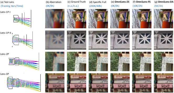
Figure 7: Visual results on synthetic data. (a): Optical paths for the test lenses. (b) and (c): The synthetic aberration images taken by the test lenses and the corresponding ground truth. (d)-(g): CAC results of compared solutions. The training iterations and time taken for dealing with a new specific lens are provided.

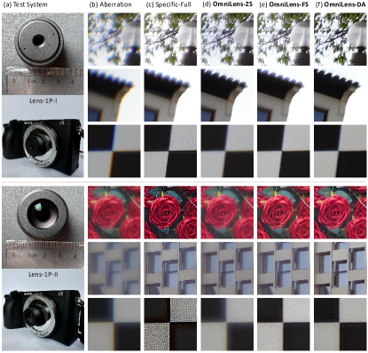
Figure 8: Visual results on real-world data. (a) The shooting device for capturing real-world images. We manufacture Lens-1P-I and Lens-1P-II and load them with a Sony ${\alpha}6600$ camera. (b)${\sim}$(f) Some test samples for real-world CAC of compared solutions.

5.1.2 Evaluation on Real-world Images

Two test lenses with more challenging optical degradation are manufactured, i.e., Lens-1P-I and Lens-1p-II, which are applied to capture around $550$ real-world aberration images respectively, as shown in Fig. 8 (a). We use $50$ images as the training data for domain adaptation while using the rest for real-world evaluation. Fig. 8 (b)${\sim}$(f) present some of the test samples. Due to the synthetic-to-real domain gap, even the lens-specific solution is unable to achieve reliable CAC results, with severe artifacts and unresolved optical degradation in the results. In this case, while the results of OmniLens-ZS deliver a few improvements compared to the un-processed aberration image, there is still significant residual optical degradation, especially for the Lens-1P-II. However, our OmniLens can provide a reliable pre-trained base model, which prevents the OmniLens-FS model from over-fitting to the synthetic lens-specific data, suppressing the artifacts. Moreover, domain adaptation shows great advantages in this case, benefiting from the directly unsupervised training on real-world aberration images. Our novel OmniLens-DA achieves impressive real-world results, completely handling the residual optical degradation without introducing visually unpleasant artifacts.

5.2 Effectiveness of AODLib

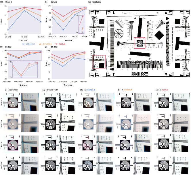
Figure 9: Evaluation of the effectiveness of AODLib via comparison with ZEBASELib and ZernikeLib. We use each LensLib to train the baseline FeMaSR model respectively for a fair comparison. (a): The overall average $Score$ of the compared LensLib pipelines on the synthetic benchmark under $3$ settings in OmniLens. (b)${\sim}$(d): The detailed $Score$ results for each lens sample. (e): The test scene using an ISO12233 resolution test chart, where we zoom in on the maximum and minimum FoV regions of the image patches to showcase the restored details. (f)${\sim}$(k): Visual results of ZS-CAC for the compared pipelines under the test scene.

The established AODLib serves as a core database to ensure convincing results of OmniLens. As shown in Fig. 9, we verify the effectiveness of AODLib via comparison with the other two LensLib pipelines, i.e., the ZEBASELib and the ZernikeLib introduced in Sec. 1. The construction process of ZEBASELib and ZernikeLib is consistent with [15] and [18] respectively. Firstly, from an overall perspective in Fig. 9 (a), AODLib delivers a clear advantage, especially in the ZS-CAC and DA-CAC settings where lens-specific data pairs are unavailable. From Fig. 9 (b)${\sim}$(d), the models trained on ZEBASELib and ZernikeLib struggle to handle cases with severe aberrations, i.e., Lens-1P-I, Lens-1P-II, and Lens-2P, where AODLib brings significant improvements over them. Consistently, the ZS-CAC’s visual results in Fig. 9 (f)${\sim}$(k) illustrate this pattern, where the CAC results of ZEBASELib and ZernikeLib still suffer from obvious optical degradation, but those of AODLib are essentially aberration-free with decent resolution.

We believe that the impressive performance of AODLib is due to its extensive coverage of aberration behaviors, which is lacking in ZEBASELib and ZernikeLib. For ZEBASELib, the trained universal model could overfit the database, as the number of manually collected samples is too small, which can hardly cover the possible aberration distributions in real-world lenses. Moreover, it is difficult to expand the size and coverage of such LensLibs, as commercial lens databases are often categorized by applications with sub-optimal structures, whose aberration behaviors are difficult to analyze and sort out manually. Despite that the ZernikeLib seems a possible solution to bath generation of virtual lens samples for a larger and broader LensLib, it overlooks the difference between the aberration distribution of the virtual lenses and real-world ones. The induced data domain gap also leads to failure cases in the CAC of unknown real-world lenses. In comparison, the coverage of our AODLib is safeguarded by the GA-based evolution framework in EAOD, while the aberration distribution is brought closer to the real-world one via the comprehensive optimization objectives and the hybrid global and local optimization strategy, making it a convincing database for universal CAC.

Table 2: Effectiveness of introduced priors. For HQCP, we compare the proposed PCM model with a U-Net model of the same architecture, where the guidance of HQCP is removed from PCM, and set the $\lambda_{DCP}$ to $0$ for domain adaptation without DCP.

Test Lens (Score)		Lens-1P-I	Lens-1P-II	Lens-2P	Lens-3P	Average
ZS-CAC	w/o HQCP	85.116	73.475	89.518	96.638	86.187
	PCM	87.644	73.981	90.377	95.345	86.837
FS-CAC	w/o HQCP	86.500	79.214	89.033	96.376	87.781
	PCM	91.518	79.288	93.988	95.942	90.184
DA-CAC	w/o HQCP	86.055	77.074	88.990	95.463	86.895
	w/o DCP	88.893	70.688	90.183	95.274	86.259
	PCM	88.848	74.973	90.378	95.445	87.409

5.3 Effectiveness of Introduced Priors

The introduced priors, i.e., the HQCP and DCP, contribute to the flexibility of our OmniLens framework, whose effectiveness is evaluated in Tab. 2. Benefiting from the learned distribution of high-quality images, HQCP first enhances the model’s generalization ability for better handling severe optical degradation, bringing superior results in ZS-CAC. Nevertheless, its greatest advantage is manifested in improving Omnilens’s flexibility. In FS-CAC and DA-CAC, HQCP can enable the model to achieve excellent results via fine-tuning in cases with limited data and training time, which is hard for the compared U-Net without any embedded priors. As in CAC, the final imaging quality is generally assigned with the top priority, making the fine-tuned model hold more value for real-world applications. In this case, HQCP is crucial for enhancing the practicality of OmniLens, as it not only saves the cost of fine-tuning but also ensures the quality of the CAC results. Moreover, we find that DCP is a universal and effective prior for the CAC task, which can provide an unsupervised constraint for domain adaptation. From the second row and the last two rows in Tab. 2, it becomes clear that only fine-tuning the model on AODLib using $\mathcal{L}_{PCM}$ leads to worse results, where directly adding the DCP constraint on the target lens images can bring significant improvements.

5.4 Ablation Study

5.4.1 AODLib Construction

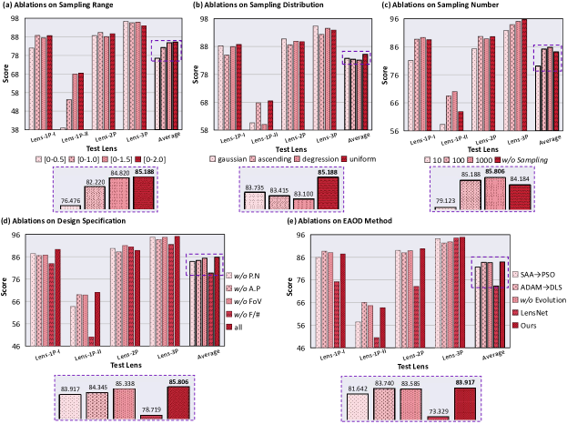
Figure 10: Ablation studies for AODLib construction. For a fair comparison, we respectively train the baseline FeMaSR model on the database generated by each ablation setting and only show the intuitive ZS-CAC results. (a): Ablations on sampling range, i.e., the $[r_{min},r_{max}]$. (b): Ablations on sampling distribution. The distribution here means the distribution of the number of samples falling into each $RMS$ interval. (c): Ablations on sampling number $N_{S}$, where the results under the un-sampled LensLib are also provided. (d): Ablations on design specification. We start from our complete EAOD framework and fix each specification individually to analyze its impact, i.e., fixing the piece number at $3$ for “$w/o$ P.N.”, the aperture position at $2$ for “$w/o$ A.P.”, the FoV at $20^{\circ}$ for “$w/o$ FoV”, and the F-number at $3.5$ for “$w/o$ F/$\#$”. (e): Ablations on EAOD method. To save experimental time, here we fix the piece number at $3$ to compare the different EAOD settings.

We first conduct ablations on the sampling strategy in AODLib construction, as shown in Fig. 10 (a)${\sim}$(c). The $N_{S}$ is set to $100$ for ablations on sampling range and distribution, whose best choice is then investigated under the optimal range and distribution. A wider $RMS$ range contributes to a larger coverage of AODLib, improving the overall performance. However, considering that it is difficult to sample enough examples with an even wider range, the $[r_{min},r_{max}]$ is set to $[0,2.0]$ for the maximum coverage possible. Then, the uniform sampling strategy is crucial for training a robust CAC model, where other sampling distributions, even increasing the proportion of samples with severe aberrations (ascending), cannot yield better results. In terms of the chosen $N_{S}$, it appears evident that sampling more samples ensures the diversity of aberration behaviors in AODLib, contributing to superior generalization ability. Yet, the improvements are marginal when $N_{S}$ is too large, where the uniform sampling becomes harder to achieve. Consequently, we set $N_{S}{=}1000$ as the final choice. Furthermore, compared with the original LensLib without sampling (“w/o $Sampling$” in Fig. 10 (c)), a reasonable sampling strategy is verified to be a necessary component in constructing AODLib, which effectively controls the aberration behaviors in LensLib to cover real-world lenses.

Table 3: Ablation study for architectures of PCM. We present the overall average $Score$ of ZS-CAC results under different architectures. The “wo” in “Fusion” means directly feeding the quantized features into the decoder for CAC. “RTB”: Residual Transformer Block in [13]. “PAB”: Permuted self-Attention Block in [39]. “RRDB”: Residual in Residual Dense Block in [38].

Fusion	Enhancement	Average Score
w/o	RSTB	71.871
Add	RSTB	86.206
Concat.	RSTB	86.674
DCN	RSTB	86.811
MCA	RSTB	86.115
SFT	RSTB	86.837
SFT	wo	81.735
SFT	RTB	81.423
SFT	PSA	84.927
SFT	RRDB	83.822

In addition, we investigate the effectiveness of components in the EAOD framework as shown in Fig. 10 (d) and (e), where the EAOD under each ablation setting is utilized to automatically design lens samples for constructing the corresponding AODLib via the aforementioned optimal sampling strategy. The participation of each specification enriches the diversity of the generated samples, thus promising superior performance, where the F-number delivers the greatest contribution. This is because, under a single F-number constraint, it is difficult to design a large number of qualified samples, limiting the coverage of the constructed AODLib. In terms of the EAOD method, the evolution mechanism in GA proves to be significant, which can still bring improvements to the results, even under the limited degrees of optimization freedom with a piece number of $3$. Then, SAA reveals clear advantages over PSO, being a superior choice for global optimization, while the results of ADAM and DLS are comparable, both being suitable for local optimization. Finally, we employ a learning-based AOD method LensNet [55] as a competing pipeline, which is fed with the same design specifications as our EAOD for a fair comparison. The proposed EAOD outperforms LensNet by a large margin in constructing the AODLib for universal CAC. This is due to the lack of strict constraints on imaging quality and physical properties in the output lens structures of a neural network, leading to a domain gap between the real-world lenses. At the same time, we find that under the same specifications, LensNet can only generate $387$ samples, far fewer than the $3746$ generated by our EAOD, thus limiting the diversity of the generated aberration behaviors.

5.4.2 Architectures of PCM

Tab. 3 shows the ablations on the architectures of the Fusion and Enhancement module in PCM. Due to the discrete nature of VQ, the direct quantized features make it difficult to restore high-quality images. Consequently, the Fusion module is crucial to unleashing the potential of HQCP, bringing tremendous improvements. In this case, most architectures in multi-modal fusion are effective, with SFT outperforming others by a slim margin. Additionally, the Enhancement module contributes to processing the deep image features before VQ, mapping them to the feature space associated with HQCP, which boosts the performance of PCM. Corroborating the conclusions in [56, 57], the RSTB delivers an advantage over other CNN and Transformer backbones in handling spatially variant optical degradation, which benefits from its ability to capture long-range dependency and the window-based mechanism to deal with local details.

6 Conclusion and Discussion

This article introduces a flexible framework OmniLens for universal CAC based on automatic LensLib generation and domain adaptation. OmniLens starts from training a base universal CAC model with strong generalization ability on a convincing lens database AODLib. This is achieved by the proposed EAOD method for automatically designing large amount lens samples, where an evolution framework is put forward to enrich the diversity of generated lens structures, and the hybrid optimization strategy equipped with comprehensive optimization objectives is employed to ensure reasonable aberration behaviors. In terms of network design, we employ the HQCP as an additional modality to guide the CAC process, which improves the zero-shot performance of the base model, while significantly contributing to superior results in the challenging few-shot setting. Experimental results on diverse lens samples demonstrate that the performance of the base universal model is comparable to that of the lens-specific model, where only fast fine-tuning on a little data is required for the universal model to outperform the lens-specific one. The base OmniLens model reveals the potential to serve as a powerful pre-trained foundation in the field of CAC, significantly elevating the ceiling of CAC models. Moreover, we develop an efficient domain adaptation method to deal with the specific lens with unknown lens descriptions, where the base model is adapted to the target lens with its unpaired aberration data. The DCP property of optical degradation is utilized to derive an unsupervised regularization term for enabling domain adaptation training. For the first time, DA is experimentally verified to be an effective and flexible solution to universal CAC, improving the base model especially when it fails in challenging lens samples.

Looking ahead, the research directions for OmniLens will focus on two key aspects. Foremost, we aim to introduce broader design flexibility into the EAOD, such as incorporating aspherical and diffractive surfaces, further expanding the coverage of the generated LensLib. Additionally, we will reframe the universal CAC task as a paradigm of emerging all-in-one image restoration, enabling the CAC model to deliver flawless performance through zero-shot inference alone. Our idea of OmniLens will benefit from the development of both automatic optical design and image restoration methods for serving as a phenomenal baseline for universal CAC.

Funding

National Key R&D Program of China, under Grant 2022YFF0705500. National Natural Science Foundation of China (No. 62473139). Henan Province Key R&D Special Project (231111112700). Hangzhou SurImage Technology Company Ltd.

Disclosures

The authors declare no conflicts of interest.

Data availability

Data underlying the results presented in this paper are not publicly available at this time but may be obtained from the authors upon reasonable request.

7 Loss Function for EAOD

7.1 Detailed Imaging Quality Constraints in EAOD

As stated in Sec. 3.1.1 of the main text, we quantify the average spot RMS radius across all sampled FoVs and wavelengths into $\mathcal{L}_{spt}$:

$$\small\mathcal{L}_{spt}=\frac{1}{n_{f}n_{w}}{\sum_{i=1}^{n_{f}}}{\sum_{j=1}^{n_{w}}}\sqrt{\frac{\sum_{k=1}^{n_{r}}[(x(i,j;k)-\overline{x(i,j)})^{2}+y(i,j;k)^{2}]}{n_{r}}}.$$ (15)

Here, $n_{f}$ represents the number of sampled FoVs, $n_{w}$ represents the number of sampled wavelengths, $n_{r}$ represents the number of sampled rays, $x(i,j;k)$ represents the image plane $x$ coordinate of the $k_{th}$ ray, traced at $i_{th}$ sampled FoV and $j_{th}$ sampled wavelength, $y(i,j;k)$ represents the image plane $y$ coordinate of the $k_{th}$ ray, traced at $i_{th}$ sampled FoV and $j_{th}$ sampled wavelength, and $\overline{x(i,j)}$ represents the $x$ coordinate of the main ray at $i_{th}$ sampled FoV and $j_{th}$ sampled wavelength. We assume that the sampled object points are all in the $x$-axis direction so $\overline{y(i,j)}{=}0$.

Then, we quantify the average lateral chromatic aberration across all sampled FoVs into $\mathcal{L}_{c}$:

$$\mathcal{L}_{c}=\frac{1}{n_{f}}{\sum_{i=1}^{n_{f}}}( \max\{\overline{x(i,1)},\overline{x(i,2)},...,\overline{x(i,n_{w})}\}-$$ (16)

$$\min\{\overline{x(i,1)},\overline{x(i,2)},...,\overline{x(i,n_{w})}\}).$$

Here, at each sampled FoV, $\mathcal{L}_{c}$ quantifies the maximum distance between main ray positions across all sampled wavelengths.

Notably, our $\mathcal{L}_{spt}$ and $\mathcal{L}_{c}$ require the support of a ray tracing model to facilitate the necessary optical calculations, which constructs the lens structure and traces the distribution of each object point on the image plane, enabling the computation of relevant spot and chromatic aberrations. We will provide a detailed description of the ray-tracing model in Sec. 8.

7.2 Detailed Physical Constraints in EAOD

In addition to the basic normalized lens parameters $P^{\mathcal{S}^{(j)}}$ (i.e., curvature, glass center thickness, air center spacing, refractive index, and abbe number) that we straightforwardly constrain the normalized values within the range $[0,1]$, other key physical properties of the lens, derived from $P^{\mathcal{S}^{(j)}}$, are constrained by a linear penalty function to fall within a reasonable range, which is quantified into $\mathcal{L}_{P}$. Physical properties constrained by $\mathcal{L}_{P}$ include effective focal length, distortion, edge spacing, glass edge thickness, back focal length, total track length, and image height. The above physical constraints are outlined in Table 4, in which $S_{FoV}$ represents half FoV and $S_{p}$ represents piece number.

Table 4: Physical constraints in EAOD.

Physical Property	Constraint Range
Curvature	$-0.1\sim 0.1$
Glass center thickness	$4mm\sim 15mm$
Air center spacing	$1mm\sim 15mm$
Refractive index	$1.51\sim 1.76$
Abbe number	$27.5\sim 71.3$
Effective Focal Length	$(\frac{14.3}{\tan(S_{FoV})}-5)mm\sim(\frac{14.3}{\tan(S_{FoV})}+5)mm$
Distortion	$-10\%\sim 10\%$
Edge Spacing	$1mm\sim 15mm$
Glass Edge Thickness	$5mm\sim 15mm$
Back Focal Length	$>15mm$
Total Track Length	$<(S_{p}\times 25+15)mm$
Image Height	$14.2mm\sim 14.4mm$

8 Imaging Simulation Model

8.1 Overall Pipeline

In our imaging simulation pipeline, the aberration-induced optical degradation is characterized by the energy dispersion of the point spread function $PSF(x^{\prime},y^{\prime})$, where $(x^{\prime},y^{\prime})$ represents image plane coordinates. Specifically, our simulation model applies the patch-wise convolution between the scene image $I_{S}$ and $PSF(x^{\prime},y^{\prime})$ for generating the aberration image $I_{A}$:

$$I_{A}(x^{\prime},y^{\prime})\approx PSF(x^{\prime},y^{\prime})\ast I_{s}(x^{\prime},y^{\prime}).$$ (17)

Besides, an optional Image Signal Processing (ISP) pipeline is introduced to help construct more realistic aberration images [58]. In this case, the scene image $I_{S}$ is replaced by the scene raw image $I^{\prime}_{S}$, and the aberration image $I_{A}$ is replaced by the aberration raw image $I^{\prime}_{A}$. Specifically, we first sequentially apply the invert gamma correction (GC), invert color correction matrix (CCM), and invert white balance (WB) to $I_{S}$ to obtain the scene raw image $I^{\prime}_{S}$. The invert ISP pipeline can be formulated as

$$I^{\prime}_{S}=P^{-1}_{WB}\circ P^{-1}_{CCM}\circ P^{-1}_{GC}(I_{S}),$$ (18)

where $\circ$ is the composition operator. $P_{WB}$, $P_{CCM}$, and $P_{GC}$ represent the procedures of WB, CCM, and GC, respectively. After conducting patch-wise convolution with the $PSF(x^{\prime},y^{\prime})$, we mosaic the degraded raw image $I^{\prime}_{A}$ before adding shot and read noise to each channel. Moreover, we sequentially apply the demosaic algorithm, i.e., WB, CCM, and GC, to the R-G-G-B noisy raw image, where the aberration-degraded image $I_{A}$ in the sRGB domain is obtained. The ISP pipeline can be defined as:

$$I_{A}=P_{GC}\circ P_{CCM}\circ P_{WB}\circ P_{demosaic}\circ(P_{mosaic}(I^{\prime}_{A})+N),$$ (19)

where $N$ represents the Gaussian shot and read noise. $P_{mosaic}$ and $P_{demosaic}$ represent the procedures of mosaicking and demosaicking respectively.

8.2 Optical Ray-Tracing Model

To obtain accurate $PSF(x^{\prime},y^{\prime})$, we build a ray-tracing-based optical model. For the sake of convenience in presentation, all the symbol notations used here are independent of the representations in the main text. The reader can simply refer to the definitions provided here to clearly understand their meanings.

For a spherical optical lens, its structure is determined by the curvatures of the spherical interfaces $c$, glass and air spacings $s$, and the refractive index $n$ and Abbe number $v$ of the material. Specifically, $n$ represents the refractive index at the “$d$” Fraunhofer line ($587.6nm$). Following [59], we use the approximate dispersion model $n({\lambda}){\approx}A{+}B{/}{\lambda}^{2}$ to retrieve the refractive index at any wavelength ${\lambda}$, where $A$ and $B$ follow the definition of the “$d$”-line refractive index and Abbe number. Thus, the lens parameters can be denoted as $\phi_{lens}{=}(c,s,n,v)$. Assuming that there is no vignetting, after the maximum field of view $\theta_{max}$ and the size of aperture stop $r_{aper}$ are determined, the ray tracing is performed. The traditional spherical surface can be expressed as:

$$z=\frac{cr^{2}}{1+\sqrt{1-c^{2}r^{2}}},$$ (20)

where $r$ indicates the distance from $(x,y)$ to the z-axis: $r^{2}{=}x^{2}{+}y^{2}$. Then, we conduct sampling on the entrance pupil. The obtained point $\textbf{S}{=}(x,y,z)$ can be regarded as a monochromatic coherent light source and its propagation direction is determined by the normalized direction vector $\textbf{D}{=}(X,Y,Z)$. The propagation process of light between two surfaces can be defined as:

$$\textbf{S}^{\prime}=\textbf{S}+t\textbf{D},$$ (21)

where $t$ denotes the distance traveled by the ray. Therefore, the process of ray tracing can be simplified as solving the intersection point $\textbf{S}^{\prime}$ of the ray and the surface, together with the direction vector $\textbf{D}^{\prime}$ after refraction. By building the simultaneous equations of Eq. 20 and Eq. 21, the solution $t$ can be acquired. After substituting $t$ into Eq. 21, the intersection point $\textbf{S}^{\prime}$ can be obtained, while the refracted direction vector $\textbf{D}^{\prime}$ can be computed by Snell’s law:

$$\textbf{D}^{\prime}=\frac{n_{1}}{n_{2}}\bigg{[}\textbf{D}+\bigg{(}\cos\langle{\textbf{p},\textbf{D}}\rangle-\sqrt{\frac{n^{2}_{2}}{n^{2}_{1}}-1+\cos^{2}\langle{\textbf{p},\textbf{D}}\rangle}\bigg{)}\textbf{p}\bigg{]},$$ (22)

where p is the normal unit vector of the surface equation, $n_{1}$ and $n_{2}$ are the refractive indices on both sides of the surface, D is the direction vector of the incident light, and $\cos\langle\cdot,\cdot\rangle$ is the operation for calculating cosine value between two vectors. By alternately calculating the intersection point $\textbf{S}^{\prime}$ and the refracted direction vector $\textbf{D}^{\prime}$, rays can be traced to the image plane to obtain the PSFs. Under dominant geometrical aberrations, diffraction can be safely ignored and the PSFs can be computed through the Gaussianization of the intersection of the ray and image plane [60]. Specifically, when the ray intersects the image plane, we get its intensity distribution instead of an intersection point. The intensity distribution of the ray on the image plane can also be described by the Gaussian function:

$$E(m,n)=\frac{1}{\sqrt{2\pi}\sigma}\exp(-\frac{r(m,n)^{2}}{2\sigma^{2}}).$$ (23)

$r(m,n)$ is the distance between the pixel indexed as $(m,n)$ and the center of the ray on the image plane, which is just the intersection point in conventional ray tracing, and $\sigma{=}\sqrt{{\Delta}x^{2}{+}{\Delta}y^{2}}/3$. By superimposing each Gaussian spot, the final PSFs can be obtained.

To sum up, the PSFs of all FoVs can be formulated as:

$$PSF(x^{\prime},y^{\prime})=T(c,s,n,v,\theta_{max},r_{aper};x^{\prime},y^{\prime}),$$ (24)

where $T(\cdot)$ refers to the setup ray tracing model. Therefore, we can produce the synthetic aberration image by feeding the lens parameters $(c,s,n,v,\theta_{max},r_{aper})$ to the imaging simulation pipeline.

8.3 Additional Details

During the imaging simulation process, to enhance the robustness of the synthetic data for addressing potential real-world scenarios, we also perform data augmentation for ISP and distortion. We first introduce ISP enhancement to obtain a new ground truth. Specifically, a set of ISP parameters is utilized to transform the image into the raw image via inverse ISP [1], which is converted into the enhanced image with the parameters perturbed by ${\pm}5\%$ via ISP. Then, the optical degradation of the selected lens is applied to the new ground truth through patch-wise convolution and noise simulation, producing the aberration image. Last but not least, distortion transformation is conducted on both the aberration image and new ground truth, constructing the final aberration-clear data pair. In this way, the paired aberration images and ground truth images in synthetic data share the same ISP offsets and distortions. The model trained on such data will only remove the optical degradation while preserving the ISP offsets and distortions. We aim to leverage this enhancement to improve the robustness of the CAC model when dealing with the presence of ISP offsets and distortions, which are common in the real-world captured images of low-end lenses.

9 More Experimental Results

Due to space constraints in the main text, we only present a subset of the metrics and results for a partial set of test cases in experiments. Here, we will provide the complete quantitative results for experiments of evaluation of OmniLens, evaluation of the effectiveness of AODLib, and evaluation of the introduced priors, in the form of tables in Tab. 5$\sim$7. Given the substantial amount of data, we recommend zooming in for the best view. Similar to that in the main text, the supplemented evaluation results also demonstrate that OmniLens provides a robust and flexible solution to the universal CAC: i) Compared to ZernikeLib and ZEBASELib, AODLib greatly enhances the generalization of the trained universal CAC model; ii) Through FS-CAC, OmniLens achieves superior results to the lens-specific model with only $5\%$ of training data and training time, where the HQCP contributes to faster convergence of the model; iii) Equipped with the unpaired aberration images, the DCP-based domain adaptation pipeline brings significant improvements to the base universal model, especially when the model fails in ZS-CAC. Finally, benefiting from the AODLib, the universal model in OmniLens can serve as a powerful pretraining model for the CAC field, contributing to raising the upper limit of lens-specific CAC.

Table 5: Detailed quantitative evaluation of OmniLens.

Test Lens	Lens-1P-I	Lens-1P-II	Lens-2P	Lens-3P	Average
	PSNR$\uparrow$/SSIM$\uparrow$/LPIPS$\downarrow$/DISTS$\downarrow$/NIQE$\downarrow$/Score$\uparrow$	PSNR$\uparrow$/SSIM$\uparrow$/LPIPS$\downarrow$/DISTS$\downarrow$/NIQE$\downarrow$/Score$\uparrow$	PSNR$\uparrow$/SSIM$\uparrow$/LPIPS$\downarrow$/DISTS$\downarrow$/NIQE$\downarrow$/Score$\uparrow$	PSNR$\uparrow$/SSIM$\uparrow$/LPIPS$\downarrow$/DISTS$\downarrow$/NIQE$\downarrow$/Score$\uparrow$	PSNR$\uparrow$/SSIM$\uparrow$/LPIPS$\downarrow$/DISTS$\downarrow$/NIQE$\downarrow$/Score$\uparrow$
Specific-FS	26.876/0.811/0.1301/0.0646/3.863/83.369	20.100/0.743/0.1736/0.0924/3.538/73.730	26.239/0.819/0.1134/0.0580/3.840/85.149	25.330/0.831/0.0916/0.0416/3.508/89.397	24.636/0.801/0.1272/0.0641/3.687/82.911
Specifc-Full	28.991/0.855/0.0748/0.0364/3.363/93.560	20.124/0.780/0.1389/0.0686/3.418/80.107	27.469/0.854/0.0937/0.0496/3.429/90.018	27.742/0.878/0.0561/0.0254/3.340/96.206	26.081/0.842/0.0909/0.0450/3.387/89.973
OmniLens-ZS	26.908/0.827/0.1116/0.0534/3.409/87.644	22.916/0.782/0.1651/0.0914/4.407/73.981	27.935/0.869/0.0942/0.0452/3.704/90.377	28.952/0.881/0.0639/0.0295/3.515/95.345	26.678/0.840/0.1087/0.0549/3.759/86.837
OmniLens-FS	28.921/0.841/0.0797/0.0400/3.654/91.518	20.354/0.782/0.1285/0.0686/3.914/79.288	29.061/0.867/0.0618/0.0325/3.741/93.988	28.852/0.886/0.0559/0.0248/3.693/95.942	26.797/0.844/0.0815/0.0415/3.750/90.184
OmniLens-DA	27.456/0.836/0.1028/0.0469/3.608/88.842	24.098/0.789/0.1606/0.0885/4.502/74.973	28.762/0.874/0.0931/0.0447/3.912/90.378	29.312/0.885/0.0607/0.0277/3.701/95.445	27.407/0.846/0.1043/0.0519/3.930/87.409
OmniLens-Full	29.318/0.853/0.0706/0.0353/3.156/94.618	20.555/0.793/0.1229/0.0628/3.476/82.066	28.873/0.875/0.0600/0.0319/3.904/93.831	28.927/0.886/0.0535/0.0238/3.499/96.809	26.918/0.852/0.0768/0.0384/3.509/91.831

Table 6: Detailed quantitative evaluation of the effectiveness of AODLib.

Test Lens	Lens-1P-I	Lens-1P-II	Lens-2P	Lens-3P	Average
	PSNR$\uparrow$/SSIM$\uparrow$/LPIPS$\downarrow$/DISTS$\downarrow$/NIQE$\downarrow$/Score$\uparrow$	PSNR$\uparrow$/SSIM$\uparrow$/LPIPS$\downarrow$/DISTS$\downarrow$/NIQE$\downarrow$/Score$\uparrow$	PSNR$\uparrow$/SSIM$\uparrow$/LPIPS$\downarrow$/DISTS$\downarrow$/NIQE$\downarrow$/Score$\uparrow$	PSNR$\uparrow$/SSIM$\uparrow$/LPIPS$\downarrow$/DISTS$\downarrow$/NIQE$\downarrow$/Score$\uparrow$	PSNR$\uparrow$/SSIM$\uparrow$/LPIPS$\downarrow$/DISTS$\downarrow$/NIQE$\downarrow$/Score$\uparrow$
ZEBASELib-ZS	23.840/0.766/0.2409/0.1155/3.974/68.159	17.708/0.610/0.4152/0.2139/6.281/32.258	23.943/0.791/0.2007/0.0968/3.858/73.789	26.163/0.860/0.0839/0.0382/3.515/91.428	22.913/0.757/0.2352/0.1161/4.407/66.409
ZEBASELib-FS	27.991/0.826/0.1020/0.0492/3.664/88.332	20.280/0.760/0.1475/0.0763/3.847/76.829	27.457/0.842/0.0918/0.0447/3.924/88.922	27.772/0.867/0.0679/0.0308/3.560/93.918	25.875/0.824/0.1023/0.0503/3.749/87.000
ZEBASELib-DA	23.218/0.758/0.2032/0.0960/3.605/73.234	20.027/0.603/0.2786/0.1539/3.760/55.381	23.524/0.782/0.1490/0.0735/3.702/79.498	26.603/0.857/0.0796/0.0368/3.497/91.975	23.343/0.750/0.1776/0.0901/3.641/75.022
ZernikeLib-ZS	24.430/0.789/0.1568/0.0728/3.383/80.752	18.206/0.711/0.2599/0.1538/4.632/56.203	24.833/0.823/0.1447/0.0713/3.695/81.803	26.867/0.850/0.0794/0.0376/3.261/92.492	23.584/0.793/0.1602/0.0839/3.743/77.812
ZernikeLib-FS	28.538/0.833/0.0884/0.0429/3.597/90.489	20.971/0.783/0.1341/0.0686/3.688/79.961	28.259/0.855/0.0755/0.0373/3.643/92.259	28.170/0.869/0.0634/0.0295/3.547/94.615	26.485/0.835/0.0903/0.0446/3.618/89.331
ZernikeLib-DA	24.543/0.773/0.1433/0.0644/3.507/81.745	20.618/0.730/0.2076/0.1194/4.207/66.231	24.875/0.818/0.1157/0.0567/3.565/85.453	27.482/0.856/0.0774/0.0369/3.654/91.923	24.380/0.794/0.1360/0.0694/3.733/81.338
AODLib-ZS	27.396/0.836/0.1062/0.0478/3.339/89.325	21.702/0.766/0.1914/0.1024/4.478/69.997	27.726/0.869/0.1080/0.0501/3.748/88.841	28.826/0.882/0.0708/0.0312/3.418/95.060	26.412/0.838/0.1191/0.0579/3.746/85.806
AODLib-FS	28.769/0.839/0.0811/0.0399/3.509/91.776	19.964/0.774/0.1339/0.0702/3.671/79.130	29.061/0.867/0.0624/0.0322/3.561/94.548	28.680/0.881/0.0574/0.0257/3.565/95.920	26.618/0.840/0.0837/0.0420/3.577/90.344
AODLib-DA	27.310/0.834/0.1015/0.0456/3.386/89.631	24.057/0.786/0.1577/0.0862/4.163/76.319	28.381/0.872/0.0991/0.0463/3.809/89.968	29.116/0.882/0.0631/0.0280/3.503/95.716	27.216/0.844/0.1054/0.0515/3.716/87.908

Table 7: Detailed quantitative evaluation of the effectiveness of the introduced priors.

Test Lens		Lens-1P-I	Lens-1P-II	Lens-2P	Lens-3P	Average
		PSNR$\uparrow$/SSIM$\uparrow$/LPIPS$\downarrow$/DISTS$\downarrow$/NIQE$\downarrow$/Score$\uparrow$	PSNR$\uparrow$/SSIM$\uparrow$/LPIPS$\downarrow$/DISTS$\downarrow$/NIQE$\downarrow$/Score$\uparrow$	PSNR$\uparrow$/SSIM$\uparrow$/LPIPS$\downarrow$/DISTS$\downarrow$/NIQE$\downarrow$/Score$\uparrow$	PSNR$\uparrow$/SSIM$\uparrow$/LPIPS$\downarrow$/DISTS$\downarrow$/NIQE$\downarrow$/Score$\uparrow$	PSNR$\uparrow$/SSIM$\uparrow$/LPIPS$\downarrow$/DISTS$\downarrow$/NIQE$\downarrow$/Score$\uparrow$
ZS-CAC	w/o HQCP	25.443/0.821/0.1194/0.0658/3.317/85.116	24.029/0.766/0.1685/0.1005/4.094/73.475	25.975/0.867/0.0892/0.0523/3.479/89.518	28.933/0.887/0.0575/0.0278/3.326/96.638	26.095/0.835/0.1086/0.0616/3.554/86.187
	PCM	26.908/0.827/0.1116/0.0534/3.409/87.644	22.916/0.782/0.1651/0.0914/4.407/73.981	27.935/0.869/0.0942/0.0452/3.704/90.377	28.952/0.881/0.0639/0.0295/3.515/95.345	26.678/0.840/0.1087/0.0549/3.759/86.837
FS-CAC	w/o HQCP	28.226/0.835/0.1105/0.0569/3.912/86.500	20.869/0.776/0.1307/0.0714/3.787/79.214	27.816/0.868/0.0922/0.0507/3.921/89.033	28.952/0.893/0.0531/0.0243/3.696/96.376	26.466/0.843/0.0966/0.0508/3.829/87.781
	PCM	28.921/0.841/0.0797/0.0400/3.654/91.518	20.354/0.782/0.1285/0.0686/3.914/79.288	29.061/0.867/0.0618/0.0325/3.741/93.988	28.852/0.886/0.0559/0.0248/3.693/95.942	26.797/0.844/0.0815/0.0415/3.750/90.184
DA-CAC	w/o HQCP	26.005/0.829/0.1123/0.0568/3.677/86.055	25.751/0.791/0.1511/0.0850/4.352/77.074	26.770/0.871/0.0903/0.0494/3.912/88.990	29.023/0.889/0.0584/0.0276/3.741/95.463	26.887/0.845/0.1030/0.0547/3.920/86.895
	w/o DCP	27.778/0.839/0.1033/0.0475/3.627/88.893	21.681/0.773/0.1815/0.0987/4.648/70.688	28.903/0.874/0.0954/0.0455/3.920/90.183	29.304/0.886/0.0623/0.0282/3.717/95.274	26.916/0.843/0.1106/0.0550/3.978/86.259
	PCM	27.456/0.836/0.1028/0.0469/3.608/88.842	24.098/0.789/0.1606/0.0885/4.502/74.973	28.762/0.874/0.0931/0.0447/3.912/90.378	29.312/0.885/0.0607/0.0277/3.701/95.445	27.407/0.846/0.1043/0.0519/3.930/87.409

References

- [1] S. Chen, H. Feng, D. Pan, et al., “Optical aberrations correction in postprocessing using imaging simulation,” \JournalTitleACM Transactions on Graphics 40, 1–15 (2021).
- [2] C. J. Schuler, M. Hirsch, S. Harmeling, and B. Schölkopf, “Non-stationary correction of optical aberrations,” in 2011 International Conference on Computer Vision (ICCV), (IEEE, 2011), pp. 659–666.
- [3] E. Kee, S. Paris, S. Chen, and J. Wang, “Modeling and removing spatially-varying optical blur,” in 2011 IEEE International Conference on Computational Photography (ICCP), (IEEE, 2011), pp. 1–8.
- [4] J. Suo, W. Zhang, J. Gong, et al., “Computational imaging and artificial intelligence: The next revolution of mobile vision,” \JournalTitleProceedings of the IEEE 111, 1607–1639 (2023).
- [5] Y. Zhang, X. Song, J. Xie, et al., “Large depth-of-field ultra-compact microscope by progressive optimization and deep learning,” \JournalTitleNature Communications 14, 4118 (2023).
- [6] F. Heide, M. Rouf, M. B. Hullin, et al., “High-quality computational imaging through simple lenses,” \JournalTitleACM Transactions on Graphics 32, 1–14 (2013).
- [7] S. Gao, L. Sun, Q. Jiang, et al., “Compact and lightweight panoramic annular lens for computer vision tasks,” \JournalTitleOptics Express 30, 29940–29956 (2022).
- [8] T. Lin, S. Chen, H. Feng, et al., “Non-blind optical degradation correction via frequency self-adaptive and finetune tactics,” \JournalTitleOptics Express 30, 23485–23498 (2022).
- [9] S. Chen, H. Feng, K. Gao, et al., “Extreme-quality computational imaging via degradation framework,” in 2021 IEEE/CVF International Conference on Computer Vision (ICCV), (IEEE, 2021), pp. 2612–2621.
- [10] S. Chen, J. Zhou, M. Li, et al., “Mobile image restoration via prior quantization,” \JournalTitlePattern Recognition Letters 174, 64–70 (2023).
- [11] J. Liang, J. Cao, G. Sun, et al., “SwinIR: Image restoration using swin transformer,” in 2021 IEEE/CVF International Conference on Computer Vision Workshops (ICCVW), (IEEE, 2021), pp. 1833–1844.
- [12] L. Chen, X. Chu, X. Zhang, and J. Sun, “Simple baselines for image restoration,” in European Conference on Computer Vision (ECCV), vol. 13667 (Springer, 2022), pp. 17–33.
- [13] S. W. Zamir, A. Arora, S. Khan, et al., “Restormer: Efficient transformer for high-resolution image restoration,” in 2022 IEEE/CVF Conference on Computer Vision and Pattern Recognition (CVPR), (IEEE, 2022), pp. 5718–5729.
- [14] S. Chen, T. Lin, H. Feng, et al., “Computational optics for mobile terminals in mass production,” \JournalTitleIEEE Transactions on Pattern Analysis and Machine Intelligence 45, 4245–4259 (2023).
- [15] J. Gong, R. Yang, W. Zhang, et al., “A physics-informed low-rank deep neural network for blind and universal lens aberration correction,” in 2024 IEEE/CVF Conference on Computer Vision and Pattern Recognition (CVPR), (IEEE, 2024), pp. 24861–24870.
- [16] X. Li, J. Suo, W. Zhang, et al., “Universal and flexible optical aberration correction using deep-prior based deconvolution,” in 2021 IEEE/CVF International Conference on Computer Vision (ICCV), (IEEE, 2021), pp. 2593–2601.
- [17] L. Hu, S. Hu, W. Gong, and K. Si, “Image enhancement for fluorescence microscopy based on deep learning with prior knowledge of aberration,” \JournalTitleOptics Letters 46, 2055–2058 (2021).
- [18] Q. Jiang, H. Shi, S. Gao, et al., “Computational imaging for machine perception: Transferring semantic segmentation beyond aberrations,” \JournalTitleIEEE Transactions on Computational Imaging 10, 535–548 (2024).
- [19] J. Sun and X. Li, “Automatic design of machine vision lens based on improved genetic algorithm and damped least squares,” in Optical Design and Testing XI, vol. 11895 (SPIE, 2021), pp. 188–202.
- [20] D. Guo, L. Yin, and G. Yuan, “New automatic optical design method based on combination of particle swarm optimization and least squares,” \JournalTitleOptics Express 27, 17027–17040 (2019).
- [21] J. Zhang, Z. Cen, and X. Li, “Automated design of machine vision lens based on the combination of particle swarm optimization and damped least squares,” in Optical Design and Testing X, vol. 11548 (SPIE, 2020), pp. 261–272.
- [22] W. Wang, H. Zhang, Z. Yuan, and C. Wang, “Unsupervised real-world super-resolution: A domain adaptation perspective,” in 2021 IEEE/CVF International Conference on Computer Vision (ICCV), (IEEE, 2021), pp. 4298–4307.
- [23] X. Xu, P. Wei, W. Chen, et al., “Dual adversarial adaptation for cross-device real-world image super-resolution,” in 2022 IEEE/CVF Conference on Computer Vision and Pattern Recognition (CVPR), (IEEE, 2022), pp. 5657–5666.
- [24] Z. Wang, L. Shen, M. Xu, et al., “Domain adaptation for underwater image enhancement,” \JournalTitleIEEE Transactions on Image Processing 32, 1442–1457 (2023).
- [25] R.-Q. Wu, Z.-P. Duan, C.-L. Guo, et al., “Ridcp: Revitalizing real image dehazing via high-quality codebook priors,” in 2023 IEEE/CVF Conference on Computer Vision and Pattern Recognition (CVPR), (IEEE, 2023), pp. 22282–22291.
- [26] C. Chen, X. Shi, Y. Qin, et al., “Real-world blind super-resolution via feature matching with implicit high-resolution priors,” in Proceedings of the 30th ACM International Conference on Multimedia (MM), (ACM, 2022), pp. 1329–1338.
- [27] J. Pan, D. Sun, H. Pfister, and M.-H. Yang, “Blind image deblurring using dark channel prior,” in 2016 IEEE Conference on Computer Vision and Pattern Recognition (CVPR), (IEEE, 2016), pp. 1628–1636.
- [28] S. Wei, H. Cheng, B. Xue, et al., “Computational imaging-based single-lens imaging systems and performance evaluation,” \JournalTitleOptics Express 32, 26107–26123 (2024).
- [29] R. A. Rutenbar, “Simulated annealing algorithms: An overview,” \JournalTitleIEEE Circuits and Devices Magazine 5, 19–26 (1989).
- [30] M. Clerc and J. Kennedy, “The particle swarm - explosion, stability, and convergence in a multidimensional complex space,” \JournalTitleIEEE Transactions on Evolutionary Computation 6, 58–73 (2002).
- [31] D. P. Kingma and J. Ba, “Adam: a method for stochastic optimization,” in International Conference on Learning Representations (ICLR), (2015).
- [32] K. Levenberg, “A method for the solution of certain non-linear problems in least squares,” \JournalTitleQuarterly of Applied Mathematics 2, 164–168 (1944).
- [33] R. Rombach, A. Blattmann, D. Lorenz, et al., “High-resolution image synthesis with latent diffusion models,” in 2022 IEEE/CVF Conference on Computer Vision and Pattern Recognition (CVPR), (IEEE, 2022), pp. 10674–10685.
- [34] J. Zhang, F. Zhan, C. Theobalt, and S. Lu, “Regularized vector quantization for tokenized image synthesis,” in 2023 IEEE/CVF Conference on Computer Vision and Pattern Recognition (CVPR), (IEEE, 2023), pp. 18467–18476.
- [35] A. van den Oord, O. Vinyals, and K. Kavukcuoglu, “Neural discrete representation learning,” in Advances in Neural Information Processing Systems (NeurIPS), vol. 30 (2017), pp. 6306–6315.
- [36] P. Esser, R. Rombach, and B. Ommer, “Taming transformers for high-resolution image synthesis,” in 2021 IEEE/CVF Conference on Computer Vision and Pattern Recognition (CVPR), (IEEE, 2021), pp. 12868–12878.
- [37] J. Ho, A. Jain, and P. Abbeel, “Denoising diffusion probabilistic models,” in Advances in Neural Information Processing Systems (NeurIPS), vol. 33 (2020), pp. 6840–6851.
- [38] X. Wang, K. Yu, S. Wu, et al., “Esrgan: Enhanced super-resolution generative adversarial networks,” in European Conference on Computer Vision (ECCV), (Springer, 2019), pp. 63–79.
- [39] Y. Zhou, Z. Li, C.-L. Guo, et al., “Srformer: Permuted self-attention for single image super-resolution,” in 2023 IEEE/CVF International Conference on Computer Vision (ICCV), (IEEE, 2023), pp. 12734–12745.
- [40] X. Zhu, H. Hu, S. Lin, and J. Dai, “Deformable convnets v2: More deformable, better results,” in 2019 IEEE/CVF Conference on Computer Vision and Pattern Recognition (CVPR), (IEEE, 2019), pp. 9300–9308.
- [41] L. Sun, C. Sakaridis, J. Liang, et al., “Event-based fusion for motion deblurring with cross-modal attention,” in European Conference on Computer Vision (ECCV), (Springer, 2022), pp. 412–428.
- [42] X. Wang, K. Yu, C. Dong, and C. C. Loy, “Recovering realistic texture in image super-resolution by deep spatial feature transform,” in 2018 IEEE/CVF Conference on Computer Vision and Pattern Recognition (CVPR), (IEEE, 2018), pp. 606–615.
- [43] R. Timofte, E. Agustsson, L. Van Gool, et al., “Ntire 2017 challenge on single image super-resolution: Methods and results,” in 2017 IEEE Conference on Computer Vision and Pattern Recognition Workshops (CVPRW), (IEEE, 2017), pp. 1110–1121.
- [44] Y. Shao, L. Li, W. Ren, et al., “Domain adaptation for image dehazing,” in 2020 IEEE/CVF Conference on Computer Vision and Pattern Recognition (CVPR), (IEEE, 2020), pp. 2805–2814.
- [45] Z. Chen, Y. Wang, Y. Yang, and D. Liu, “Psd: Principled synthetic-to-real dehazing guided by physical priors,” in 2021 IEEE/CVF Conference on Computer Vision and Pattern Recognition (CVPR), (IEEE, 2021), pp. 7176–7185.
- [46] Q. Jiang, Y. Zhang, F. Bao, et al., “Two-step domain adaptation for underwater image enhancement,” \JournalTitlePattern Recognition 122, 108324 (2022).
- [47] K. He, J. Sun, and X. Tang, “Single image haze removal using dark channel prior,” \JournalTitleIEEE Transactions on Pattern Analysis and Machine Intelligence 33, 2341–2353 (2011).
- [48] Q. Jiang, H. Shi, L. Sun, et al., “Annular computational imaging: Capture clear panoramic images through simple lens,” \JournalTitleIEEE Transactions on Computational Imaging 8, 1250–1264 (2022).
- [49] J. Liang, R. Timofte, Q. Yi, et al., “Ntire 2024 restore any image model (raim) in the wild challenge,” in 2024 IEEE/CVF Conference on Computer Vision and Pattern Recognition (CVPR), (IEEE, 2024), pp. 6632–6640.
- [50] Z. Wang, A. C. Bovik, H. R. Sheikh, and E. P. Simoncelli, “Image quality assessment: from error visibility to structural similarity,” \JournalTitleIEEE Transactions on Image Processing 13, 600–612 (2004).
- [51] R. Zhang, P. Isola, A. A. Efros, et al., “The unreasonable effectiveness of deep features as a perceptual metric,” in 2018 IEEE/CVF Conference on Computer Vision and Pattern Recognition (CVPR), (IEEE, 2018), pp. 586–595.
- [52] K. Ding, K. Ma, S. Wang, and E. P. Simoncelli, “Image quality assessment: Unifying structure and texture similarity,” \JournalTitleIEEE Transactions on Pattern Analysis and Machine Intelligence 44, 2567–2581 (2020).
- [53] A. Mittal, R. Soundararajan, and A. C. Bovik, “Making a “completely blind”’ image quality analyzer,” \JournalTitleIEEE Signal Processing Letters 20, 209–212 (2012).
- [54] A. Paszke, S. Gross, F. Massa, et al., “PyTorch: An imperative style, high-performance deep learning library,” in Advances in Neural Information Processing Systems (NeurIPS), vol. 32 (2019), pp. 8024–8035.
- [55] G. Côté, J.-F. Lalonde, and S. Thibault, “Deep learning-enabled framework for automatic lens design starting point generation,” \JournalTitleOptics Express 29, 3841–3854 (2021).
- [56] Q. Jiang, S. Gao, Y. Gao, et al., “Minimalist and high-quality panoramic imaging with psf-aware transformers,” \JournalTitleIEEE Transactions on Image Processing 33, 4568–4583 (2024).
- [57] A. Jaiswal, X. Zhang, S. H. Chan, and Z. Wang, “Physics-driven turbulence image restoration with stochastic refinement,” in 2023 IEEE/CVF International Conference on Computer Vision (ICCV), (IEEE, 2023), pp. 12136–12147.
- [58] T. Brooks, B. Mildenhall, T. Xue, et al., “Unprocessing images for learned raw denoising,” in 2019 IEEE/CVF Conference on Computer Vision and Pattern Recognition (CVPR), (IEEE, 2019), pp. 11028–11037.
- [59] Q. Sun, C. Wang, Q. Fu, et al., “End-to-end complex lens design with differentiate ray tracing,” \JournalTitleTOG 40, 1–13 (2021).
- [60] Z. Li, Q. Hou, Z. Wang, et al., “End-to-end learned single lens design using fast differentiable ray tracing,” \JournalTitleOL 46, 5453–5456 (2021).