State estimation of timed automata under partial observation

Abstract

In this paper, we consider partially observable timed automata endowed with a single clock. A time interval is associated with each transition specifying at which clock values it may occur. In addition, a resetting condition associated to a transition specifies how the clock value is updated upon its occurrence. This work deals with the estimation of the current state given a timed observation, i.e., a succession of pairs of an observable event and the time instant at which the event has occurred. The problem of state reachability in the timed automaton is reduced to the reachability analysis of the associated zone automaton, which provides a purely discrete event description of the behaviour of the timed automaton. An algorithm is formulated to provide an offline approach for state estimation of a timed automaton based on the assumption that the clock is reset upon the occurrence of each observable transition.

Keywords: Discrete event system, timed automaton, state estimation.

1 Introduction

In the area of discrete event systems (DES), a large body of literature considers logical DES, where time is abstracted and only the order of occurrences of the events is taken into account. The problem of state estimation has received a lot of attention considering different observation structures in different formalisms, in particular automata [1] and Petri nets [2]. The notion of observer [3] contains all the information to reconstruct the set of current states consistent with an observation and allows to move most of the burdensome parts of the computations offline and can be used for online state estimation. In addition, an observer is fundamental to address problems of feedback control [4], diagnosis and diagnosability [5], [6], in addition to characterizing a large set of dynamical properties, such as detectability [7], opacity [8] and resilience to cyber-attack [9].

Significant contributions have also been provided in the framework of timed DES. As an example, in [10], observers are designed for a particular class of weighted automata, where the time information of transition firability is given to weights. References [11], [12], [13], and [14] address the problem of state estimation of a class of timed automata under a rather restrictive scenario where the endowed single clock is reset to zero after each event occurrence. The state estimation of timed DES has also been considered in [15] and [16], but no general approach concerning the construction of an observer for a general class of timed DES exists.

Another active area of research is that of hybrid systems (HS) [17, 18], characterized by the interplay between discrete event and time-driven dynamics. These systems can be modeled by hybrid automata, and in particular by timed automata [19] concerning time elapsing as time-driven dynamics. State estimation of timed automata has also been studied. In [19], the reachability of locations can be analysed by searching the finite quotient of a timed automaton with respect to the region equivalence defined over the set of all clock interpretations. However, the reachability is analyzed regardless of any observations. Tripakis proposes an online diagnoser in [20] that keeps track of all the possible discrete states. Thereby, state estimation problem is theoretically solvable. In [21] and [22], timed markings are used for representing the closure under silent transitions. Observe that in [20, 21, 22], only online estimators have been proposed, and no general approach concerning the construction of an observer is known. In particular the model we consider in this paper, that we call timed finite automaton can be either seen as a finite state automaton endowed with a clock or as a timed automaton [19] whose edges are labeled.

A related problem in a decentralized setting is studied in [23], where the asynchronous polling of distributed sub-systems is called synchronization. Concerning timed automata, references [24], [25], and [26] discuss how to define concurrent composition for timed automata, which can be used to construct complex models.

This paper considers a partially observable timed finite automaton (TFA) endowed with a single clock. The logical structure specifies the sequences of events that the TFA can generate and the observations they produce. The timed structure specifies the set of clock values that allow an event to occur and how the clock is reset upon the event occurrence. A timed state of a TFA consists of a discrete state associated with the logical structure and the clock value. Our objective is that of estimating the current discrete state of the automaton as a function of the current observation and of the current time. The notion of $T$-reachability is proposed taking into account which discrete states can be reached with an evolution that produces a given observation and has a duration equal to $T$. We prove that the problem of $T$-reachability for a TFA is reduced to the reachability analysis of the associated zone automaton. We assume that the firing of observable transitions resets the clock to a set that is a finite union of zones, and present a formal approach that allows one to construct offline an observer, i.e., a finite structure that describes the state estimation for all possible evolutions. During the online phase to estimate the current discrete state, one just has to determine which is the state of the observer reached by the current observation and check to which interval (among a finite number of time intervals) the time elapsed between the last observed event occurrence belongs. We believe that the proposed approach has a major advantage over existing online approaches for state estimation: it paves the way to address a vast range of fundamental properties (detectability, opacity, etc.) that have so far mostly been studied in the context of logical DES.

The rest of the paper is organized as follows. Section II introduces the background of DES, timed automata and time semantics. Section III formally state the problem of state estimation. Section IV illustrates the approaches to compute zones and to construct the zone automaton. Section V provides necessary and sufficient conditions for the reachability of a state of the timed automaton in terms of reachability analysis in the zone automaton. Section VI solves the problem of updating the state estimation according to the latest received timed observation. Finally, Section VII concludes this paper.

2 Background

A nondeterministic finite automaton (NFA) is a four-tuple $G=(X,E,\Delta,X_{0})$, where $X$ is a finite set of states, $E$ is a finite set of events, $\Delta\subseteq X\times E\times X$ is the transition relation and $X_{0}\subseteq X$ is the set of initial states. The set of events $E$ can be partitioned as $E=E_{o}\dot{\cup}E_{uo}$, where $E_{o}$ is the set of observable events, and $E_{uo}$ is the set of unobservable events. We denote by $E^{\ast}$ the set of all finite strings on $E$, including the empty word $\varepsilon$. The concatenation $s_{1}\cdot s_{2}$ of two strings $s_{1}\in E^{\ast}$ and $s_{2}\in E^{\ast}$ is a string consisting of $s_{1}$ immediately followed by $s_{2}$. The empty string $\varepsilon$ is an identity element of concatenation, i.e., for any string $s\in E^{\ast}$, it holds that $\varepsilon\cdot s=s=s\cdot\varepsilon$. Given a string in $E^{\ast}$, the observation is defined via the observation projection $P_{l}:E^{\ast}\longrightarrow E_{o}^{\ast}$ defined as: $P_{l}(\varepsilon)=\varepsilon$, and for all $s\in E^{\ast}$ and $e\in E$, it is $P_{l}(s\cdot e)=P_{l}(s)\cdot e$ if $e\in E_{o}$, or $P_{l}(s\cdot e)=P_{l}(s)$ if $e\in E_{uo}$.

Let $\mathbb{R}_{\geq 0}$ be the set of non-negative real numbers and $\mathbb{N}$ be the set of natural numbers. A closed interval, i.e., closed on both sides, is denoted as $[m,n]$, while open or semi-open intervals are denoted as $(m,n)$, $[m,n)$ or $(m,n]$. We denote the set of all time intervals and the set of all closed time intervals as $\mathbb{I}$ and $\mathbb{I}_{c}$, respectively, where $\mathbb{I}_{c}\subseteq\mathbb{I}$. The addition of $I_{1}$ and $I_{2}$ is defined as $I_{1}\bigoplus I_{2}=\{t_{1}+t_{2}\in\mathbb{R}_{\geq 0}\mid t_{1}\in I_{1},t_{2}\in I_{2}\}$ and the distance range between them as $D(I_{1},I_{2})=\{|t_{1}-t_{2}|\ \mid t_{1}\in I_{1},t_{2}\in I_{2}\}$.

Definition 1.

A timed finite automaton (TFA) is a six-tuple $G=(X$, $E$, $\Delta$, $\Gamma$, $Reset$, $X_{0})$ that operates under a single clock, where $X$ is a finite set of discrete states, $E$ is an alphabet, $\Delta\subseteq X\times E\times X$ is a transition relation, $\Gamma:\Delta\rightarrow\mathbb{I}_{c}$ is a timing function, $Reset:\Delta\rightarrow\mathbb{I}_{c}\cup\{id\}$ is a clock resetting function such that for $\delta\in\Delta$, the clock is reset to be an integer value in a time interval $I\in\mathbb{I}_{c}$ ($Reset(\delta)=I$), or the clock is not reset ($Reset(\delta)=id$), and $X_{0}\subseteq X$ is the set of initial discrete states. $\square$

For the sake of simplicity, we assume that the clock is set to be 0 initially. A transition $(x,e,x^{\prime})\in\Delta$ denotes that the occurrence of event $e\in E$ leads to $x^{\prime}\in X$ when the TFA is at $x\in X$. The time interval $\Gamma((x,e,x^{\prime}))$ specifies a range of clock values at which the event $e$ may occur, while $Reset((x,e,x^{\prime}))\in\mathbb{I}_{c}$ denotes the range of the clock values that are reset to be and $Reset((x,e,x^{\prime}))=id$ implies that the clock is not reset. The set of output transitions at $x$ is defined as $O(x)=\{(x,e,x^{\prime})\in\Delta\mid e\in E,x^{\prime}\in X\}$, and the set of input transitions at $x$ is defined as $I(x)=\{(x^{\prime},e,x)\in\Delta\mid e\in E,x^{\prime}\in X\}$.

A timed state is defined as a pair $(x,\theta)\in X\times\mathbb{R}_{\geq 0}$, where $\theta$ is the current value of the clock. In other words, a timed state $(x,\theta)$ keeps track of the current clock assignment $\theta$ while $G$ stays at state $x$. The behaviour of a TFA is described via its timed runs. A timed run $\rho$ of length $k\geq 0$ from $t_{0}\in\mathbb{R}_{\geq 0}$ to $t_{k}\in\mathbb{R}_{\geq 0}$ is a sequence of $k+1$ timed states $(x_{(i)},\theta_{(i)})\in X\times\mathbb{R}_{\geq 0}\ (i=0,\cdots,k)$, and $k$ pairs $(e_{i},t_{i})\in E\times\mathbb{R}_{\geq 0}\ (i=1,\cdots,k)$, represented as $\rho:(x_{(0)},\theta_{(0)}){\xrightarrow{(e_{1},t_{1})}}\cdots(x_{(k-1)},\theta_{(k-1)}){\xrightarrow{(e_{k},t_{k})}}(x_{(k)},\theta_{(k)})$ such that $(x_{(i-1)},e_{i},x_{(i)})\in\Delta$, and the following conditions hold for all $i=1,\cdots,k$:

• $\theta_{(i)}\in Reset((x_{(i-1)},e_{i},x_{(i)}))$ and $\theta_{(i-1)}+t_{i}-t_{i-1}\in\Gamma((x_{(i-1)},e_{i},x_{(i)}))$, if $Reset((x_{(i-1)},e_{i},x_{(i)}))\neq id$;

• $\theta_{(i)}=\theta_{(i-1)}+t_{i}-t_{i-1}\in\Gamma((x_{(i-1)},e_{i},x_{(i)}))$, if $Reset((x_{(i-1)},e_{i},x_{(i)}))=id$.

We define the timed word generated by $\rho$ as $\sigma(\rho)=(e_{1},t_{1})(e_{2},t_{2})\cdots(e_{k}$, $t_{k})\in(E\times\mathbb{R}_{\geq 0})^{\ast}$. We also define the logical word generated by $\rho$ as $S(\sigma(\rho))=e_{1}e_{2}\cdots e_{k}$ via a function defined as $S:(E\times\mathbb{R}_{\geq 0})^{\ast}\rightarrow E^{\ast}$. For the timed run of length 0 as $\rho:(x_{(0)},\theta_{(0)})$, we have $S(\sigma(\rho))=\varepsilon$ and $\sigma(\rho)=\lambda$, where $\lambda$ denotes the empty timed word in $E\times\mathbb{R}_{\geq 0}$. For the timed word $\sigma(\rho)$ generated from an arbitrary timed run $\rho$, it is $\lambda\cdot\sigma(\rho)=\sigma(\rho)=\sigma(\rho)\cdot\lambda$. The starting discrete state and the ending discrete state of a timed run $\rho$ are denoted by $x_{st}(\rho)=x_{(0)}$ and $x_{en}(\rho)=x_{(k)}$, respectively. The starting time and the ending time of $\rho$ are denoted by $t_{st}(\rho)=t_{0}$ and $t_{en}(\rho)=t_{k}$, respectively. In addition, the duration of $\rho$ is denoted as $T(\rho)=t_{k}-t_{0}$. The set of timed runs generated by $G$ is denoted as $\mathcal{R}(G)$.

A timed evolution of $G$ from $t_{0}\in\mathbb{R}_{\geq 0}$ to $t\in\mathbb{R}_{\geq 0}$ is defined by a pair $(\sigma(\rho),t)\in(E\times\mathbb{R}_{\geq 0})^{\ast}\times\mathbb{R}_{\geq 0}$, where $t_{st}(\rho)=t_{0}$ and $t_{en}(\rho)\leq t$. Note that $t-t_{en}(\rho)$ is the time that the system stays at the ending discrete state $x_{en}(\rho)$. Furthermore, we denote as $\mathcal{E}(G,t)=\{(\sigma(\rho),t)\mid(\exists\rho\in\mathcal{R}(G))\ x_{st}(\rho)\in X_{0},t_{st}(\rho)=0,t_{en}(\rho)\leq t\}$ the timed language of $G$ from $0$ to $t\in\mathbb{R}_{\geq 0}$, that contains all possible timed evolutions of $G$ from $0$ to $t$.

Definition 2.

Given a TFA $G=(X,E,\Delta,\Gamma,Reset,X_{0})$ and a time instant $T\in\mathbb{R}_{\geq 0}$, a discrete state $x^{\prime}\in X$ is said to be $T$-reachable from $x\in X$ if there exists a timed evolution $(\sigma(\rho),t)\in(E\times\mathbb{R}_{\geq 0})^{\ast}\times\mathbb{R}_{\geq 0}$ of $G$ such that $t-t_{st}(\rho)=T$, $x_{st}(\rho)=x$, and $x_{en}(\rho)=x^{\prime}$. In addition, $x^{\prime}$ is said to be unobservably $T$-reachable from $x$ if $x^{\prime}$ is $T$-reachable from $x$ with a timed evolution $(\sigma(\rho),t)$ such that $S(\sigma(\rho))\in E_{uo}^{\ast}$. $\square$

In simple words, $x^{\prime}$ is $T$-reachable from $x$ if a timed evolution leads the system from $x$ to $x^{\prime}$ with an elapsed time $T$. If there exists such a timed evolution that produces no observation, $x^{\prime}$ is unobservably $T$-reachable from $x$.

Example 1.

Given a TFA $G=(X$, $E$, $\Delta$, $\Gamma$, $Reset$, $X_{0})$ in Fig. 1(a) with $X=\{x_{0},x_{1},x_{2},x_{3},x_{4}\}$, $E=\{a,b,c\}$, $\Delta=\{(x_{0},c,x_{1})$, $(x_{0},b,x_{2})$, $(x_{1},a,x_{4})$, $(x_{2},c,x_{3})$, $(x_{3},a,x_{2})$, $(x_{4},b,x_{3})\}$, the initial state in $X_{0}=\{x_{0}\}$ is marked by an input arrow. The information given by the timing function $\Gamma$ and the clock resetting function $Reset$ defined in Fig. 1(b) is presented on the edges. Given an edge denoting a transition $\delta\in\Delta$, the label $\theta\in\Gamma(\delta)?$ on the edge specifies if $\delta$ is enabled with respect to $\theta$; the label $\theta:\in Reset(\delta)$ (resp., $\theta:=id$) on the edge specifies to which range $\theta$ belongs (resp., specifies that the clock is not reset) after the transition is fired. Consider a timed run $\rho:(x_{0},0)\stackrel{{\scriptstyle(b,0.5)}}{{\longrightarrow}}(x_{2},0.5)\stackrel{{\scriptstyle(c,2)}}{{\longrightarrow}}(x_{3},2)\stackrel{{\scriptstyle(a,2)}}{{\longrightarrow}}(x_{2},0)$ that starts from $x_{st}(\rho)=x_{0}$ at $t_{st}(\rho)=0$ and terminates in $x_{en}(\rho)=x_{2}$ at $t_{en}(\rho)=2$. Three transitions $(x_{0},b,x_{2})$, $(x_{2},c,x_{3})$, and $(x_{3},a,x_{2})$ occur at time instants $t_{1}=0.5$, $t_{2}=2$ and $t_{3}=2$, respectively. The transitions $(x_{0},b,x_{2})$ and $(x_{2},c,x_{3})$ do not lead the clock to be reset, while $(x_{3},a,x_{2})$ resets the clock to $0$. Given a timed evolution $(\sigma(\rho),2)$, it follows that $x_{2}$ and $x_{3}$ are $2$-reachable from $x_{0}$. $\square$

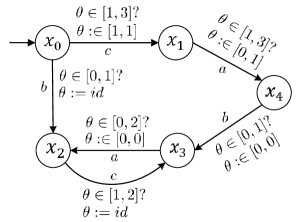
(a) A TFA $G$.

$\delta\in\Delta$	$\Gamma(\delta)$	$Reset(\delta)$
$(x_{0},c,x_{1})$	$[1,3]$	$[1,1]$
$(x_{0},b,x_{2})$	$[0,1]$	$id$
$(x_{1},a,x_{4})$	$[1,3]$	$[0,1]$
$(x_{2},c,x_{3})$	$[1,2]$	$id$
$(x_{3},a,x_{2})$	$[0,2]$	$[0,0]$
$(x_{4},b,x_{3})$	$[0,1]$	$[0,0]$

(b) Timing function and clock resetting function.

Figure 1: A TFA $G$ w.r.t. the given timing function and clock resetting function.

3 Problem Statement

In this work we model a partially observed timed plant as a TFA $G=(X,E,\Delta,\Gamma,Reset,X_{0})$ with a partition of the alphabet into observable and unobservable events: $E=E_{o}\dot{\cup}E_{uo}$. Next we preliminarily define a projection function on timed words.

Definition 3.

Given a TFA $G$ with $E=E_{o}\dot{\cup}E_{uo}$, a projection function $P:(E\times\mathbb{R}_{\geq 0})^{\ast}\longrightarrow(E_{o}\times\mathbb{R}_{\geq 0})^{\ast}$ is defined as $P(\lambda)=\lambda$, and $P(\sigma(\rho)\cdot(e,t))=P(\sigma(\rho))$ if $e\in E_{uo}$, or $P(\sigma(\rho)\cdot(e,t))=P(\sigma(\rho))\cdot(e,t)$ if $e\in E_{o}$, for the timed word $\sigma(\rho)\in(E\times\mathbb{R}_{\geq 0})^{\ast}$ generated from any timed run $\rho\in\mathcal{R}(G)$ and for all $(e,t)\in E\times\mathbb{R}_{\geq 0}$. Given a timed evolution $(\sigma(\rho),t)$, the pair $(\sigma_{o},t)=(P(\sigma(\rho)),t)$ is said to be the timed observation. $\square$

Definition 4.

Given a TFA $G$ with $E=E_{o}\dot{\cup}E_{uo}$, and a timed observation $(\sigma_{o},t)$, $\mathcal{S}(\sigma_{o},t)=\{(\sigma(\rho),t)\in\mathcal{E}(G,t)|P(\sigma(\rho))=\sigma_{o}\}$ is said to be the set of timed evolutions consistent with $(\sigma_{o},t)$, i.e., the set of timed evolutions that can be generated by $G$ from $0$ to $t$ producing the timed observation $(\sigma_{o},t)$; meanwhile $\mathcal{X}(\sigma_{o},t)=\{x_{en}(\rho)\in X|(\sigma(\rho),t)\in\mathcal{S}(\sigma_{o},t)\}$ is said to be the set of discrete states consistent with $(\sigma_{o},t)$, i.e., the set of discrete states in which $G$ may be, after $(\sigma_{o},t)$ is observed. $\square$

This work aims at calculating the set $\mathcal{X}(\sigma_{o},t)$, which includes the discrete states reached by each timed evolution $(\sigma(\rho),t)$ consistent with $(\sigma_{o},t)$. In addition, this work also provides a range of the possible clock values associated with each timed evolution $(\sigma(\rho),t)$.

4 Zone automaton

The notion of zone automaton has been introduced in [13] to provide a purely discrete event description of the behaviour of a given timed automaton endowed with a single clock reset at each event occurrence and bounded by the maximal dwell time at each discrete state. The zones associated with a discrete state $x$ partition the clock values at $x$. The timed automaton in [13] can be seen as a particular case of the TFA in this paper. In this section, a new algorithm is provided to compute the zones associated with a given discrete state. After that, we illustrate how to construct the zone automaton based on the zone automaton in [13]. We first introduce the following definitions.

Definition 5.

The set of regions of a discrete state $x\in X$ is defined as $R(x)=\{[m_{x},m_{x}],(m_{x},m_{x}+1),[m_{x}+1,m_{x}+1],(m_{x}+1,m_{x}+2),\cdots$, $[M_{x},M_{x}]\}$, where $m_{x}$ (resp., $M_{x}$) is the minimal (resp., maximal) integer in $\{\Gamma(\delta)|\delta\in O(x)\vee(\delta\in I(x),Reset(\delta)=id)\}\cup\{Reset(\delta)\neq id|\delta\in I(x)\}.\hfill\square$

The integer $m_{x}$ (resp., $M_{x}$) represents the minimal (resp., maximal) clock value that can enable an output transition at $x$ and that can reach $x$ by an input transition. Note that for a transition $\delta$ inputting state $x$, we search minimal (resp., maximal) value in $\Gamma(\delta)$ if $\delta$ does not reset the clock or $Reset(\delta)$ if $\delta$ resets the clock. The regions of $x$ include the integers from $m_{x}$ to $M_{x}$ and the open segments between the integers. Given $r=[k,k]\in R(x)$ (resp., $r=(k,k+1)\in R(x)$), where $k=m_{x},\cdots,M_{x}-1$, its successive region is denoted as $succ(r)=(k,k+1)$ (resp., $succ(r)=[k+1,k+1]$). For instance, given the discrete state $x_{0}$ of the TFA $G$ in Fig. 1, we have $m_{x_{0}}=0$ , $M_{x_{0}}=3$, and $R(x_{0})=\{[0,0],(0,1),[1,1],\cdots,[3,3]\}$.

Definition 6.

Given a TFA $G=(X$, $E$, $\Delta$, $\Gamma$, $Reset$, $X_{0})$, the set of output transitions at $(x,r)\in X\times\bigcup\limits_{x\in X}R(x)$ is defined as $O(x,r)=\{(x,e,x^{\prime})\in\Delta|e\in E,x^{\prime}\in X,r\subseteq\Gamma((x,e,x^{\prime}))\}$, and the set of input transitions at $(x,r)$ is defined as $I(x,r)=\{(x^{\prime},e,x)\in\Delta\mid e\in E,(r\subseteq Reset((x^{\prime},e,x))\neq id)\vee(Reset((x^{\prime},e,x))=id,r\subseteq\Gamma((x^{\prime},e,x)))\}$. Obviously, $O(x)=\bigcup\limits_{r\in R(x)}O(x,r)$ and $I(x)=\bigcup\limits_{r\in R(x)}I(x,r)$. $\hfill\square$

The set of output (resp., input) transitions at a timed state $(x,r)$ includes all the transitions that can fire from $x$ (resp. reach $x$) with a clock value in $r$. Based on this definition, Algorithm 1 merges the regions $r_{k},r_{k+1},\cdots,r_{k^{\prime}}\in R(x)$ into a zone if the following conditions hold for $i=k+1,\cdots,k^{\prime}$: (a) $r_{i}=succ(r_{i-1})$; (b) $I(x,r_{k})=I(x,r_{i})$, $O(x,r_{k})=O(x,r_{i})$; (c) $Reset(\delta)\neq id$ for all $\delta\in I(x,r_{i})\cup O(x,r_{i})$. For a region $r\in R(x)$ and a transition $\delta\in I(x,r)\cup O(x,r)$ such that $Reset(\delta)=id$, the region $r$ is included in $Z(x)$ and no merge is done with other regions.

The set of zones $Z(x)$ partition the clock values $[0,+\infty)$ at $x$ into disjoint segments according to the firability of the input and output transitions. The maximum number of zones at $x$ is denoted as $Q_{x}=2(M_{x}-m_{x})+1$. Note that the partition of zones according to Algorithm 1 is not optimal, one can find a more compact partition by further merging the zones associated with $\delta$ where $Reset(\delta)=id$.

Input: A TFA $G=(X,E,\Delta,\Gamma,Reset,X_{0})$, a discrete state $x\in X$

Output: The set of zones $Z(x)$

1 Initialization: let $m=m_{x}$, $M=M_{x}$, $r=[m,m]$, $z=r$, $Z(x)=\emptyset$ 

2while $r\neq[M,M]$ do

3       let $r^{\prime}=succ(r)$

4      if $[O(x,r)=O(x,r^{\prime})]\wedge[I(x,r)=I(x,r^{\prime})]\wedge[(\forall\delta\in O(x,r^{\prime})\cup I(x,r^{\prime}))Reset(\delta)\neq id]$ then

5             let $z=z\cup r^{\prime}$

6      

7      else

8             let $Z(x)=Z(x)\cup\{z\}$ and $z=r^{\prime}$

9      let $r=r^{\prime}$

let $Z(x)=Z(x)\cup\{z\}\cup\{(M,+\infty)\}$

Algorithm 1 Computation of the set of zones $Z(x)$

Example 2.

Consider the TFA $G$ in Fig. 1. Algorithm 1 provides the set of zones $Z(x_{0})=\{[0,0],(0,1),[1,1],(1,3],(3,+\infty)\}$. In detail, the regions $[0,0],(0,1),[1,1]$ remain in $Z(x_{0})$ and do not merge with other regions due to $Reset((x_{0},b,x_{2}))=id$. The zone $(1,3]$ is obtained by merging the regions $(1,2)$, $[2,2]$, $(2,3)$ and $[3,3]$, which satisfy the if condition in line 4 of Algorithm 1.$\hfill\square$

Definition 7 ([13]).

Consider a TFA $G=(X,E,\Delta,\Gamma,X_{0})$ with a single clock that is reset at each event occurrence. The zone automaton of $G$ is an NFA $ZA(G)=(V,E_{\tau},\Delta_{z},V_{0})$, where

• $V\subseteq X\times\bigcup\limits_{x\in X}Z(x)$ is the finite set of extended states,

• $E_{\tau}\subseteq E\cup\{\tau\}$ is the alphabet, where the event $\tau$ implies time elapsing from any clock value $\theta\in z$ to any $\theta^{\prime}\in succ(z)$ when $G$ stays at $x\in X$;

• $\Delta_{z}\subseteq V\times E_{\tau}\times V$ is the transition relation,

• $V_{0}=\{(x,[0,0])\mid x\in X_{0}\}\subseteq V$ is the set of initial extended states.$\hfill\square$

The work in [13] corresponds to the particular case with $Reset(\delta)=[0,0]$ for each transition $\delta\in\Delta$ and a maximal dwell time for each discrete state. The zone automaton is a finite state automaton that provides a purely discrete event description of the behaviour of a given timed automaton. Each state of a zone automaton is called an extended state, which is a pair $(x,z)$ whose first element is a discrete state $x\in X$ and whose second element is a zone $z\in Z(x)$ specifying the range of the clock values. The extended state evolves either because of the elapsed time $\tau$ or because of the occurrence of a discrete event. In the former, a transition $((x,z),\tau,(x,succ(z)))\in\Delta_{z}$ corresponds to a time-driven evolution of $G$ from a clock value in $z$ to another clock value in $succ(z)\in Z(x)$. In the latter, an event-driven evolution caused by an event $e\in E$ from $(x,z)$ leads to $(x^{\prime},z^{\prime})$ indicating that the occurrence of event $e$ yields $x^{\prime}$ with a clock value in $z^{\prime}$.

In this paper, the zone automaton associated with a TFA can be constructed by implementing the event-driven evolution according to both the timing function and the clock resetting function. In detail, for each transition $(x,e,x^{\prime})\in\Delta$, we first determine whether $z\subseteq\Gamma((x,e,x^{\prime}))$; if so, for each zone $z^{\prime}\in Z(x^{\prime})$, a transition $((x,z),e,(x^{\prime},z^{\prime}))$ is defined if (a) $Reset((x,e,x^{\prime}))\neq id$ and $z^{\prime}\subseteq Reset((x,e,x^{\prime}))$ (the clock is reset after $(x,e,x^{\prime})$ occurs), or if (b) $Reset((x,e,x^{\prime}))=id$ and $z=z^{\prime}$ (the clock is not reset after $(x,e,x^{\prime})$ occurs). We further define the function $f_{x}:V\rightarrow X$ (resp., $f_{z}:V\rightarrow\bigcup\limits_{x\in X}Z(x)$) mapping an extended state in $V$ to a discrete state in $X$ (resp., a zone of the associated discrete state).

Example 3.

Consider the TFA $G=(X$, $E$, $\Delta$, $\Gamma$, $Reset$, $X_{0})$ in Fig. 1. The zone automaton $G_{z}=(V,E_{\tau},\Delta_{z},V_{0})$ is shown in Fig. 2. For instance, transition $((x_{0},[0,0]),\tau,(x_{0},(0,1)))$ implies that the clock may evolve from $0$ to any value in $(0,1)$ if $G$ is at $x_{0}$. Three transitions labeled with $b$ go from $(x_{0},[0,0])$ to $(x_{2},[0,0])$, from $(x_{0},(0,1))$ to $(x_{2},(0,1))$, and from $(x_{0},[1,1])$ to $(x_{2},[1,1])$, respectively. Each transition implies an event-driven evolution from $x_{0}$ to $x_{2}$ under the occurrence of a transition $(x_{0},b,x_{2})$.$\hfill\square$

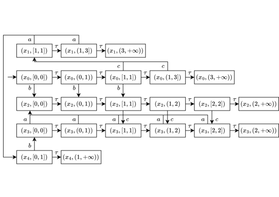
Figure 2: Zone automaton $G_{z}$ of the TFA $G$ in Fig. 1.

5 Dynamics of a zone automaton

In this section, we explore the dynamics of a zone automaton $G_{z}=(V,E_{\tau},\Delta_{z}$, $V_{0})$ associated with a TFA $G=(X,E,\Delta,\Gamma,Reset,X_{0})$ and discuss how the timed evolutions of $G$ are related to the evolutions of zone automaton $G_{z}$.

Definition 8.

Given a zone automaton $G_{z}=(V$, $E_{\tau}$, $\Delta_{z}$, $V_{0})$ and a discrete state $x$ of a TFA $G$, a $\tau$-run at $x$ of length $k\ (1\leq k\leq n)$ is defined as a sequence of $k$ extended states $(x,z_{(i)})\in V\ (i=1,\cdots,k)$, and event $\tau\in E_{\tau}$, represented as $\rho_{\tau}(x):(x,z_{(1)})\stackrel{{\scriptstyle\tau}}{{\longrightarrow}}\cdots\stackrel{{\scriptstyle\tau}}{{\longrightarrow}}(x,z_{(k)})$ such that $((x,z_{(i)}),\tau,(x,z_{(i+1)}))\in\Delta_{z}$ holds for $i\in\{1,\cdots,k-1\}$. The starting extended state and the ending extended state of $\rho_{\tau}(x)$ are denoted as $v_{st}(\rho_{\tau}(x))=(x,z_{(1)})$ and $v_{en}(\rho_{\tau}(x))=(x,z_{(k)})$, respectively. The duration range of $\rho_{\tau}(x)$ is the time distance of $z_{(1)}$ and $z_{(k)}$, denoted as $d(\rho_{\tau}(x))=D(z_{(1)},z_{(k)})$.$\hfill\square$

Definition 9.

Given a zone automaton $G_{z}=(V$, $E_{\tau}$, $\Delta_{z}$, $V_{0})$ of a TFA $G$, a run of length $k\geq 0$ is a sequence of $k+1$ $\tau$-runs $\rho_{\tau}(x_{(i)})\ (i=0,\cdots,k)$ at $x_{(i)}\in X$, and $k$ events $e_{i}\in E\ (i=1,\cdots,k)$, represented as $\bar{\rho}:\rho_{\tau}(x_{(0)})\stackrel{{\scriptstyle e_{1}}}{{\longrightarrow}}\rho_{\tau}(x_{(1)})\cdots\stackrel{{\scriptstyle e_{k}}}{{\longrightarrow}}\rho_{\tau}(x_{(k)}),$ such that $(v_{en}(\rho_{\tau}(x_{(i-1)})),e_{i},v_{st}(\rho_{\tau}(x_{(i)})))\in\Delta_{z}$ holds for $i\in\{1,\cdots,k\}$. In addition, the starting extended state and the ending extended state of $\bar{\rho}$ are defined as $v_{st}(\bar{\rho})=v_{st}(\rho_{\tau}(x_{(0)}))$ and $v_{en}(\bar{\rho})=v_{en}(\rho_{\tau}(x_{(k)}))$, respectively. The duration range of $\bar{\rho}$ is defined as $d(\bar{\rho})=\bigoplus\limits_{i=1}^{k}d(\rho_{\tau}(x_{i}))$. The logical word generated by $\bar{\rho}$ is denoted as $s(\bar{\rho})=e_{1}\cdots e_{k}$ via a function defined as $s:E_{\tau}^{\ast}\rightarrow E^{\ast}$. The set of runs generated by $G_{z}$ is defined as $\mathcal{R}_{z}(G_{z})$. $\square$

The dynamics of a zone automaton $G_{z}$ can be represented by its runs, each of which is a sequence of $\tau$-runs, which implies the time elapses discretely at discrete states, connected by an evolution caused by an event $e_{i}\in E$. We now provide a sufficient and necessary condition for the reachability of a discrete state in a TFA and explain the correlation of the dynamics of a TFA and that of zone automaton.

Theorem 1.

Given a TFA $G=(X,E,\Delta,\Gamma,Reset,X_{0})$, zone automaton $G_{z}=(V,E_{\tau},\Delta_{z},V_{0})$ and a time instant $T\in\mathbb{R}_{\geq 0}$, $x^{\prime}\in X$ is $T$-reachable from $x\in X$ if and only if there exists a run $\bar{\rho}$ in $G_{z}$ such that $T\in d(\bar{\rho})$, $v_{st}(\bar{\rho})=(x,z)$, and $v_{en}(\bar{\rho})=(x^{\prime},z^{\prime})$, where $z\in Z(x)$ and $z^{\prime}\in Z(x^{\prime})$.

Proof.

(if) Let $x=x_{(0)}$, $x^{\prime}=x_{(k)}$, $t_{0}$, $t_{1},\cdots,t_{k}\in\mathbb{R}_{\geq 0}$ and $\bar{\rho}:\rho_{\tau}(x_{(0)}){\xrightarrow{e_{1}}}\cdots{\xrightarrow{e_{k}}}$ $\rho_{\tau}(x_{(k)})$ be a run such that $e_{i}\in E$, $t_{i}-t_{i-1}\in d(\rho_{\tau}(x_{(i-1)}))$ for $i\in\{1,\cdots,k\}$, $t-t_{k}\in d(\rho_{\tau}(x_{(k)}))$, and $T=t-t_{0}\in d(\bar{\rho})$. It can be inferred that $(v_{en}(\rho_{\tau}(x_{(i-1)})),e_{i},v_{st}(\rho_{\tau}(x_{(i)})))\in\Delta_{z}$ holds for $i\in\{1,\cdots,k\}$. Accordingly, for $i\in\{1,\cdots,k\}$, there exist $\theta_{(i-1)}+t_{i}-t_{i-1}\in f_{z}(v_{en}(\rho_{\tau}(x_{(i-1)})))$ and $\theta_{(i)}\in f_{z}(v_{st}(\rho_{\tau}(x_{(i)})))$ such that $(x_{(i-1)},e_{i},x_{(i)})\in O(x_{(i-1)},f_{z}(v_{st}(\rho_{\tau}(x_{(i-1)}))))$ and $(x_{(i-1)},e_{i},x_{(i)})\in I(x_{(i)},f_{z}(v_{st}(\rho_{\tau}(x_{(i)}))))$. It is obvious that there exists a timed evolution $(\sigma(\rho),t)$, where the timed run $\rho$:$(x_{(0)},\theta_{(0)}){\xrightarrow{(e_{1},t_{1})}}$ $\cdots$ ${\xrightarrow{(e_{k},t_{k})}}(x_{(k)}$, $\theta_{(k)})$ satisfies the condition $T(\rho)=t_{k}-t_{0}$. Thus, $x^{\prime}$ is $T$-reachable from $x$.

(only if) Let $(\sigma(\rho),t)\in(E\times\mathbb{R}_{\geq 0})^{\ast}\times\mathbb{R}_{\geq 0}$ be a timed evolution of $G$ from $t_{0}\in\mathbb{R}_{\geq 0}$ to $t\in\mathbb{R}_{\geq 0}$ such that $x_{st}(\rho)=x$ and $x_{en}(\rho)=x^{\prime}$. The proof is made by induction on the length $k$ of the timed run $\rho$ generated by $G$ from $t_{0}$ to $t$. The base case is for the timed run $\rho$ of length 0 that involves only the discrete state $x$ and no transition in $G$. It is $\sigma(\rho)=\lambda$ and $x_{st}(\rho)=x_{en}(\rho)=x=x^{\prime}$. There exists a run $\bar{\rho}:(x,\bar{z})\stackrel{{\scriptstyle\tau}}{{\longrightarrow}}\cdots\stackrel{{\scriptstyle\tau}}{{\longrightarrow}}(x,z)$ in $G_{z}$, where $T=t-t_{0}\in d(\bar{\rho})$. Thus the base case holds. By denoting $x=x_{(0)}$ and $x^{\prime}=x_{(k)}$, the induction hypothesis is that the existence of a timed evolution $(\sigma(\rho),t)$ generating from $t_{0}$, where $\rho:(x_{(0)},\theta_{(0)}){\xrightarrow{(e_{1},t_{1})}}\cdots{\xrightarrow{(e_{k},t_{k})}}(x_{(k)},\theta_{(k)})$ of length $k\geq 1$ with $x_{(i)}\in X$ and $e_{i}\in E$ for all $i\in\{1,\cdots,k\}$, implies the existence of a run $\bar{\rho}:\rho_{\tau}(x_{(0)}){\xrightarrow{e_{1}}}\cdots{\xrightarrow{e_{k}}}\rho_{\tau}(x_{(k)})$ in $G_{z}$ such that $t-t_{0}\in d(\bar{\rho})$, $t-t_{k}\in d(\rho_{\tau}(x_{(k)}))$, $t_{i}-t_{i-1}\in d(\rho_{\tau}(x_{(i-1)}))$ for $i\in\{1,\cdots,k\}$, $v_{st}(\bar{\rho})=(x_{(0)},z)$ and $v_{en}(\bar{\rho})=(x_{(k)},\bar{z})$, where $z\in Z(x_{(0)})$, and $\bar{z}\in Z(x_{(k)})$. We now prove that the same implication holds for a timed evolution $(\sigma(\rho^{\prime}),t^{\prime})$, where $\rho^{\prime}$: $\rho{\xrightarrow{(e_{k+1},t)}}(x_{(k+1)},\theta_{(k+1)})$. According to $\rho^{\prime}$, it is $\theta_{(k+1)}\in Reset((x_{(k)}$, $e_{k+1}$, $x_{(k+1)}))$ if $Reset((x_{(k)},e_{k+1},x_{(k+1)}))\neq id$, or $\theta_{(k+1)}\in\Gamma((x_{(k)},e_{k+1},x_{(k+1)}))$ if $Reset((x_{(k)},e_{k+1},x_{(k+1)}))=id$. In addition, $\theta_{(k)}+t-t_{k}\in\Gamma((x_{(k)},e_{k+1},x_{(k+1)}))$. It implies that there exists a run $\bar{\rho}^{\prime}:\bar{\rho}{\xrightarrow{e_{k+1}}}\rho_{\tau}(x_{({k+1})})$ in $G_{z}$ such that $\theta_{(k+1)}\in f_{z}(v_{st}(\rho_{\tau}(x_{({k+1})})))$ and $\theta_{(k+1)}+t^{\prime}-t\in f_{z}(v_{en}(\rho_{\tau}(x_{({k+1})})))$. Therefore, it is $t^{\prime}-t_{0}\in d(\bar{\rho}^{\prime})$ according to $t^{\prime}-t\in d(\rho_{\tau}(x_{({k+1})})))$ and $t-t_{0}\in d(\bar{\rho})$. ∎

According to Theorem 1, if $x^{\prime}$ is $T$-reachable from $x$, then in the zone automaton $G_{z}$ there exists a run that originates from $(x,z)$ and reaches $(x^{\prime},z^{\prime})$, where $z\in Z(x)$ and $z^{\prime}\in Z(x^{\prime})$. In addition, $T$ belongs to the duration range of that run. In turn, given a run $\bar{\rho}$ in $G_{z}$ such that $T\in d(\bar{\rho})$, it can be concluded that the discrete state associated with $v_{en}(\bar{\rho})$ is $T$-reachable from the discrete state associated with $v_{st}(\bar{\rho})$. In simple words, the $T$-reachability of $x^{\prime}$ from $x$ can be analyzed by exploring an appropriate run in the zone automaton.

Example 4.

Consider the TFA $G$ in Fig. 1 and zone automaton $G_{z}$ in Fig. 2. A timed evolution $((c,1.5)(a,3),4)$ of $G$ from $0$ to $4$ implies that $x_{4}$ is $4$-reachable from $x_{0}$, which can be concluded from a run in $G_{z}$ as $\bar{\rho}:\rho_{\tau}(x_{0})\stackrel{{\scriptstyle c}}{{\longrightarrow}}\rho_{\tau}(x_{1})\stackrel{{\scriptstyle a}}{{\longrightarrow}}\rho_{\tau}(x_{4})$, where $\rho_{\tau}(x_{0}):(x_{0},[0,0]))\stackrel{{\scriptstyle\tau}}{{\longrightarrow}}(x_{0},(0,1))\stackrel{{\scriptstyle\tau}}{{\longrightarrow}}$$(x_{0},[1,1])$$\stackrel{{\scriptstyle\tau}}{{\longrightarrow}}(x_{0},(1,3])$, $\rho_{\tau}(x_{1}):(x_{1},[1,1])\stackrel{{\scriptstyle\tau}}{{\longrightarrow}}(x_{1},(1,3])$ and $\rho_{\tau}(x_{4}):(x_{4},[0,1]).$ $\square$

6 State estimation of TFA

Given a partially observed TFA $G=(X$, $E$, $\Delta$, $\Gamma$, $Reset$, $X_{0})$ with a partition of alphabet $E=E_{o}\dot{\cup}E_{uo}$, in this section we develop an approach for state estimation based on the zone automaton $G_{z}$, given a timed observation $(\sigma_{o},t)\in(E_{o}\times\mathbb{R}_{\geq 0})^{\ast}\times\mathbb{R}_{\geq 0}$.

We partition this section into two subsections. In the first subsection, we consider the case where $G$ produces no observation, which is an intermediate step towards the solution of the state estimation problem under partial observation. In the second subsection, we take into account the information coming from the observation of new events at certain time instants, and prove that the discrete states consistent with a timed observation $(\sigma_{o},t)$ and the range of clock value associated with each estimated discrete state can be inferred following a finite number of runs in the zone automaton $G_{z}$. We make the following assumption.

Assumption 1 (RO: Reinitialized observations).

The clock is reset upon the occurrence of any observable event, i.e.,

$$(x,e,x^{\prime})\in\Delta,\ e\in E_{o}\quad\Longrightarrow\quad Reset(x,e,x^{\prime})\neq id.$$

$\hfill\square$

This assumption is necessary to ensure that the defined zone automaton contains all relevant information to estimate the discrete state. Consider a scenario where an observable event occurs without resetting the clock. In such a case, for future estimations one may need to keep track of this exact value adding new extended states to the zone automaton: thus, the state space of the zone automaton could grow indefinitely as new events are observed.

6.1 State estimation under no observation

Definition 10.

Given a TFA $G=(X$, $E$, $\Delta$, $\Gamma$, $Reset$, $X_{0})$ with set of unobservable events $E_{uo}$ and zone automaton $G_{z}=(V,E_{\tau},\Delta_{z},V_{0})$, the following set of extended states $V_{\lambda}(x,z,t)=\{v_{en}(\bar{\rho})\in V\mid(\exists\bar{\rho}\in\mathcal{R}_{z}(G_{z}))t\in d(\bar{\rho}),v_{st}(\bar{\rho})=(x,z),s(\bar{\rho})\in E_{uo}^{\ast}\}$ is said to be $\lambda$-estimation from $(x,z)\in V$ within $t\in\mathbb{R}_{\geq 0}$. $\square$

Given a zone automaton, the $\lambda$-estimation from $(x,z)\in V$ within $t\in\mathbb{R}_{\geq 0}$ is the set of extended states of $G_{z}$ that can be reached following a run of duration $t$, originating at $(x,z)$ and producing no observation. If $(x^{\prime},z^{\prime})\in V_{\lambda}(x,z,t)$, it basically reveals that $x^{\prime}$ is unobservably $T$-reachable from $x$ with a clock value $\theta\in z$ according to Theorem 1. In addition, the zone $z^{\prime}$ associated with $x^{\prime}$ specifies the range of the value of the clock. The $\lambda$-estimation from $(x,z)$ within $t$ can be obtained by enumerating the runs starting from $(x,z)$ with a duration associated with $t$. By denoting the maximum number of zones for $x\in X$ as $Q_{x}$, the complexity for computing the $\lambda$-estimation is $\mathcal{O}(q^{3}|X|)$ with $q=\max\limits_{x\in X}|Q_{x}|$.

Proposition 1.

Given a TFA with a set of discrete states $X$, the set of unobservable events $E_{uo}$, and zone automaton $G_{z}=(V,E_{\tau},\Delta_{z},V_{0})$, $x^{\prime}\in X$ is unobservably $T$-reachable from $x\in X$, where $T\in\mathbb{R}_{\geq 0}$, if and only if there exist $z\in Z(x)$ and $z^{\prime}\in Z(x^{\prime})$ such that $(x^{\prime},z^{\prime})\in V_{\lambda}(x,z,T)$.

Proof.

(if) Suppose that there exist $z\in Z(x)$ and $z^{\prime}\in Z(x^{\prime})$ such that $(x^{\prime},z^{\prime})\in V_{\lambda}(x,z,T)$. There exists a run $\bar{\rho}$ in $G_{z}$ such that $v_{st}(\bar{\rho})=(x,z)$, $v_{en}(\bar{\rho})=(x^{\prime},z^{\prime})$, $s(\bar{\rho})\in E_{uo}^{\ast}$ and $T\in d(\bar{\rho})$. According to Theorem 1, $x^{\prime}$ is unobservably $T$-reachable from $x$.

(only if) Let $x^{\prime}$ be unobservably $T$-reachable from $x$. Then, there exists a timed evolution $(\sigma(\rho),t)$ from $t_{0}$ such that $x_{st}(\rho)=x$, $x_{en}(\rho)=x^{\prime}$, $T=t-t_{0}$, and $s(\bar{\rho})\in E_{uo}^{\ast}$. Accordingly, there exists a run $\bar{\rho}$ in $G_{z}$ such that $v_{st}(\bar{\rho})=(x,z)$, $v_{en}(\bar{\rho})=(x^{\prime},z^{\prime})$, $s(\bar{\rho})\in E_{uo}^{\ast}$ and $T\in d(\bar{\rho})$, where $z\in Z(x)$ and $z^{\prime}\in Z(x^{\prime})$. Thus, $(x^{\prime},z^{\prime})\in V_{\lambda}(x,z,T)$. ∎

Table 1: State estimation of the TFA $G$ in Fig. 1 under no observation for $t\in[0,2]$.

$k$	Time interval $I_{k}$	$\lambda$-estimation $V_{\lambda}(x_{0},[0,0],t)$, where $t\in I_{k}$	$\mathcal{X}(\lambda,t),t\in I_{k}$
$0$	[0,0]	$\{(x_{0},[0,0]),(x_{2},[0,0])\}$	$\{x_{0},x_{2}\}$
$1$	(0,1)	$\{(x_{0},(0,1)),(x_{2},(0,1))\}$	$\{x_{0},x_{2}\}$
$2$	[1,1]	$\{(x_{0},[1,1]),(x_{1},[1,1]),(x_{2},[1,1]),(x_{3},[1,1])\}$	$\{x_{0},x_{1},x_{2},x_{3}\}$
$3$	(1,2)	$\{(x_{0},(1,3]),(x_{1},[1,1]),(x_{1},(1,3]),(x_{2},(1,2)),(x_{3},(1,2))\}$	$\{x_{0},x_{1},x_{2},x_{3}\}$
$4$	[2,2]	$\{(x_{0},(1,3]),(x_{1},[1,1]),(x_{1},(1,3]),(x_{2},[2,2]),(x_{3},[2,2])\}$	$\{x_{0},x_{1},x_{2},x_{3}\}$

Example 5.

Consider the TFA $G$ in Fig. 1, where $E_{o}=\{a\}$, $E_{uo}=\{b,c\}$, and zone automaton $G_{z}$ in Fig. 2. Given the following runs in $G_{z}$ of duration 1 starting from $(x_{0},[0,0])$ and involving no observable events: (1) $\bar{\rho}_{1}:\rho_{\tau}(x_{0})$; (2) $\bar{\rho}_{2}:\rho_{\tau}(x_{0})\stackrel{{\scriptstyle c}}{{\longrightarrow}}\rho_{\tau}(x_{1})$; (3) $\bar{\rho}_{3}:\rho_{\tau}(x_{0})\stackrel{{\scriptstyle b}}{{\longrightarrow}}\rho_{\tau}(x_{2})$; and (4) $\bar{\rho}_{4}:\rho_{\tau}(x_{0})\stackrel{{\scriptstyle b}}{{\longrightarrow}}\rho_{\tau}(x_{2})\stackrel{{\scriptstyle c}}{{\longrightarrow}}\rho_{\tau}(x_{3})$, where $\rho_{\tau}(x_{0}):(x_{0},[0,0])\stackrel{{\scriptstyle\tau}}{{\longrightarrow}}(x_{0},(0,1))\stackrel{{\scriptstyle\tau}}{{\longrightarrow}}(x_{0},[1,1])$, $\rho_{\tau}(x_{1}):(x_{1},[1,1])$, $\rho_{\tau}(x_{2}):(x_{2},[1,1])$, and $\rho_{\tau}(x_{3}):(x_{3},[1,1])$, it can be inferred that $V_{\lambda}(x_{0},[0,0],1)=\{(x_{0},[1,1]),(x_{1},[1,1]),(x_{2},[1,1]),(x_{3},[1,1])\}$. Table 1 summarizes the $\lambda$-estimation and the set of discrete states consistent with $(\lambda,t)$, where $t$ belongs to a region of $[0,2]$.$\hfill\square$

6.2 State estimation under partial observation

In this subsection we focus on the most general state estimation problem when a timed observation is received as a pair of a non-empty timed word and a time instant. We first propose a general result that characterizes the set of discrete states of a TFA consistent with a given timed observation, by means of the extended states reachable in zone automaton.

Theorem 2.

Consider a TFA $G=(X$, $E$, $\Delta$, $\Gamma$, $Reset$, $X_{0})$ with set of observable events $E_{o}$. Given a timed observation $(\sigma_{o},t)\in(E_{o}\times\mathbb{R}_{\geq 0})^{\ast}\times\mathbb{R}_{\geq 0}$, it is $x\in\mathcal{X}(\sigma_{o},t)$ if and only if there exists a run $\bar{\rho}$ in the zone automaton $G_{z}$ such that $f_{x}(v_{st}(\bar{\rho}))\in X_{0}$, $f_{x}(v_{en}(\bar{\rho}))=x$, $t\in d(\bar{\rho})$ and $P_{l}(s(\bar{\rho}))=S(\sigma_{o})$, where $P_{l}:E^{\ast}\rightarrow E_{o}^{\ast}$.

Proof.

(if) In the case that no observation is contained in $\sigma_{o}$, let $\bar{\rho}:\rho_{\tau}(x_{0})$ be a run in $G_{z}$, where $x_{0}\in X_{0}$. We have $f_{x}(v_{en}(\bar{\rho}))=x_{0}$, $t\in d(\bar{\rho})$ and $\sigma_{o}=\lambda$. In this case there exists only one timed evolution $(\lambda,t)\in\mathcal{E}(G,t)$ such that $x_{0}\in\mathcal{X}(\lambda,t)$. In the case that there exist one or more event occurrences, let us suppose that $x_{(0)}\in X_{0}$, $x_{(k)}=x$, and a run in $G_{z}$ as $\bar{\rho}:\rho_{\tau}(x_{(0)}){\xrightarrow{e_{1}}}\cdots{\xrightarrow{e_{k}}}\rho_{\tau}(x_{(k)})$ such that $t\in d(\bar{\rho})$, $x_{(i)}\in X$ and $e_{i}\in E$ for $i\in\{0,\cdots,k\}$. It can be inferred that there exists a timed evolution $(\sigma(\rho),t)$ such that $x_{(k)}$ is $t$-reachable from $x_{(0)}$, where the timed run $\rho:(x_{(0)},\theta_{(0)}){\xrightarrow{(e_{1},t_{1})}}\cdots{\xrightarrow{(e_{k},t_{k})}}(x_{(k)},\theta_{(k)})$ satisfies for $i\in\{1,\cdots,k\}$ that $t-t_{k}\in d(\rho_{\tau}(x_{(k)}))$, $t_{i}-t_{i-1}\in d(\rho_{\tau}(x_{(i-1)}))$, $\theta_{(i-1)}+t_{i}-t_{i-1}\in\Gamma((x_{(i-1)},e_{i},x_{(i)}))$ , $\theta_{(i)}\in Reset((x_{(i-1)},e_{i},x_{(i)}))$ if $Reset((x_{(i-1)},e_{i},x_{(i)}))\neq id$, and $\theta_{(i)}\in\Gamma((x_{(i-1)},e_{i},x_{(i)}))$ if $Reset((x_{(i-1)},e_{i},x_{(i)}))=id$. According to $P_{l}(\bar{s}(\bar{\rho}))=S(\sigma_{o})$, we have $(\sigma(\rho),t)\in\mathcal{S}(\sigma_{o},t)$. Obviously, $x\in\mathcal{X}(\sigma_{o},t)$ holds.

(only if) In the case that $\sigma_{o}=\lambda$, $x\in\mathcal{X}(\lambda,t)$ holds. There exists a run $\bar{\rho}$ in $G_{z}$ such that $x$ is unobservably $t$-reachable from $x_{0}\in X_{0}$. Consequently, $f_{x}(v_{en}(\bar{\rho}))=x$, $t\in d(\bar{\rho})$ and $\bar{s}(\bar{\rho})=\varepsilon$ hold. In the case that $\sigma_{o}=(e_{o1},t_{1})\cdots(e_{ok},t_{k})$, where $k\geq 1$, $0\leq t_{1}\leq\cdots\leq t_{k}\leq t$ and $e_{oi}\in E_{o}\ (i\in\{1,\cdots,k\})$, it is $x\in\mathcal{X}(\sigma_{o},t)$, implying that $x$ is $t$-reachable from $x_{0}\in X_{0}$. Consequently, there exists a run $\bar{\rho}$ in $G_{z}$ such that $t\in d(\bar{\rho})$, $f_{x}(v_{st}(\bar{\rho}))=x_{0}$ and $f_{x}(v_{en}(\bar{\rho}))=x$. Let $\bar{\rho}$ be a sequence of $k$ runs $\bar{\rho}_{i}$ and $k$ observable events $e_{oi}$, where $i\in\{1,\cdots,k\}$, as $\bar{\rho}:\bar{\rho}_{0}{\xrightarrow{e_{o1}}}\cdots{\xrightarrow{e_{ok}}}\bar{\rho}_{k}$. Obviously, $\bar{s}(\bar{\rho})=e_{o1}\cdots e_{ok}$, $t-t_{k}\in d(\bar{\rho}_{k})$ and $t_{i}-t_{i-1}\in d(\bar{\rho}_{i-1})$ hold for each $i\in\{1,\cdots,k\}$. ∎

In simple words, $x\in\mathcal{X}(\sigma_{o},t)$ if there exists a run $\bar{\rho}$ in $G_{z}$ that produces the same logical observation as $\sigma_{o}$ from a discrete state in $X_{0}$ at $0$ and reaches $x$ at $t$. In turn, $x\in\mathcal{X}(\sigma_{o},t)$ can be computed following run $\bar{\rho}$ in $G_{z}$.

Proposition 2.

Consider a TFA $G$ with set of observable events $E_{o}$ that produces two timed observations $(\sigma_{o},t_{i}),(\sigma_{o},t)\in(E_{o}\times\mathbb{R}_{\geq 0})^{\ast}\times\mathbb{R}_{\geq 0}$, where $\sigma_{o}=(e_{o1},t_{1})\cdots(e_{oi},t_{i})$ and $t_{1}\leq\cdots\leq t_{i}\leq t$ for $i\geq 1$. For each timed state $(x,\theta)$ reached by a timed evolution in $\mathcal{S}(\sigma_{o},t_{i})$, and for each $v\in V_{\lambda}(x,z,t-t_{i})$, where $z\in Z(x)$ and $\theta\in z$, it holds $f_{x}(v)\in\mathcal{X}(\sigma_{o},t)$ if Assumption RO holds.

Proof.

Let a timed run $\rho:(x_{0},0)\xrightarrow{(e_{1},t_{1})}(x_{(1)},\theta_{(1)})\cdots\xrightarrow{(e_{k},t_{k})}(x_{(k)},\theta_{(k)})\xrightarrow{(e_{oi},t_{i})}(x,\theta)$, where $x_{(1)},\cdots,x_{(k)}\in X$, $e_{1},\cdots,e_{k}\in E$, and $P(\sigma(\rho))=\sigma_{o}$, the timed state $(x,\theta)$ is reached by the timed evolution $(\sigma(\rho),t_{i})\in\mathcal{S}(\sigma_{o},t_{i})$. According to Theorem 1, it can be inferred that there exists a run in $G_{z}$ as $\bar{\rho}:(x_{0},[0,0])\rightarrow\cdots\rightarrow(x,z)$, where $\theta\in z$. If Assumption RO holds, it implies that there exists $z\in Z(x)$ such that $\theta\in z$ and $z\subseteq Reset((x_{(k)},e_{oi},x))$. Given $v\in V_{\lambda}(x,z,t-t_{i})$, there exists a run $\bar{\rho}^{\prime}:(x,z)\rightarrow\cdots\rightarrow v$ such that $P_{l}(s(\bar{\rho}^{\prime}))=\varepsilon$ and $t-t_{i}\in d(\bar{\rho}^{\prime})$. Given $\bar{\rho}$ and $\bar{\rho}^{\prime}$, it can be inferred that $f_{x}(v)\in\mathcal{X}(\sigma_{o},t)$ according to Theorem 2. ∎

This proposition shows that the state estimation can be updated by computing associated $\lambda$-estimations under Assumption RO. In other words, given $(x,\theta)$ reached by a timed evolution in $\mathcal{X}(\sigma_{o},t_{i})$, $\mathcal{X}(\sigma_{o},t)$ can be inferred by computing $V_{\lambda}(x,z,t-t_{i})$, where $z\in Z(x)$ and $\theta\in z$.

Based on the previous results, Algorithm 2 summarizes the proposed approach to compute $\mathcal{X}(\sigma_{o},t)$. Consider a timed observation $(\sigma_{o},t)$ with $\sigma_{o}=(e_{o1},t_{1})\cdots(e_{on},t_{n})\ (n\geq 1)$, where $e_{o1},\cdots,e_{on}\in E_{o}$. The timed observation $(\sigma_{o},t)$ is updated whenever an observable event $e_{oi}$ occurs at a time instant $t_{i}$, where $i\in\{1,\cdots,n\}$. The algorithm provides the estimated states via a set of extended states $V_{\lambda}\subseteq V$ while time elapses in $[t_{i-1},t_{i}]$ with no event being observed, in addition to a set of extended states $\bar{V}_{i}\subseteq V$ of $G_{z}$ consistent with each new observation $(e_{oi},t_{i})$, where $i\in\{1,\cdots,n\}$ and $t_{0}=0$. Initially, it is imposed $\bar{V}_{0}=V_{0}$ and $\bar{V}_{i}=\emptyset$ for all $i\in\{1,\cdots,n\}$. Then, for any $i\in\{1,\cdots,n\}$, the algorithm computes the $\lambda$-estimation from an extended state $(\bar{x},\bar{z})\in\bar{V}_{i-1}$ within $t_{i}-t_{i-1}$ implying the discrete states unobservably $(t_{i}-t_{i-1})$-reachable from $\bar{x}$ with a clock value in $\bar{z}$, and the set $\bar{V}_{i}$ is updated with the extended states reached by transitions labeled with $e_{oi}$ from the extended states in $V_{\lambda}$. After the set $\bar{V}_{n}$ is determined, we initialize $V_{\lambda}$ to be empty and update $V_{\lambda}$ by including the $\lambda$-estimation for each $(\bar{x},\bar{z})\in\bar{V}_{n}$ within $t-t_{n}$. Finally, we return the set of discrete states of $G$ associated with $V_{\lambda}$ as the set of discrete states consistent with $(\sigma_{o},t)$.

Input: A TFA $G$ with a set of initial discrete states $X_{0}$, a set of observable events $E_{o}\subseteq E$, a zone automaton $G_{z}=(V,E_{\tau},\Delta_{z},V_{0})$, and a timed observation $(\sigma_{o},t)$ from $0$ to $t\in\mathbb{R}_{\geq 0}$, where $\sigma_{o}=(e_{o1},t_{1})\cdots(e_{on},t_{n})\ (n\geq 1)$ and $t_{1},\cdots,t_{n}\in\mathbb{R}_{\geq 0}$

Output: A set of discrete states $\mathcal{X}(\sigma_{o},t)$

1

2let $\bar{V}_{0}=V_{0}$, $t_{0}=0$ and $X_{\lambda}=\emptyset$ 

3for each $i\in\{1,\cdots,n\}$  do

4       let $e=e_{oi}$, $\bar{V}_{i}=\emptyset$ and $V_{\lambda}=\emptyset$ 

5      for each $(\bar{x},\bar{z})\in\bar{V}_{i-1}$ do

6            compute $V_{\lambda}(\bar{x},\bar{z},t_{i}-t_{i-1})$ 

7            let $V_{\lambda}=V_{\lambda}\cup V_{\lambda}(\bar{x},\bar{z},t_{i}-t_{i-1})$ 

8      

9      for each $v\in V_{\lambda}$ do

10             let $x=f_{x}(v)$ and $z=f_{z}(v)$ 

11            if $\exists x^{\prime}\in X$ s.t. $z\subseteq\Gamma((x,e,x^{\prime}))$ then

12                   for each $z^{\prime}\in Z(x^{\prime})$ s.t. $z^{\prime}\subseteq Reset((x,e,x^{\prime}))$ do

13                         let $\bar{V}_{i}=\bar{V}_{i}\cup\{(x^{\prime},z^{\prime})\}$ 

14                  

15            

16      

17let $V_{\lambda}=\emptyset$ 

18for each $(\bar{x},\bar{z})\in\bar{V}_{n}$ do

19       compute $V_{\lambda}(\bar{x},\bar{z},t-t_{n})$  

20      let $V_{\lambda}=V_{\lambda}\cup V_{\lambda}(\bar{x},\bar{z},t-t_{n})$ 

21

return $\mathcal{X}(\sigma_{o},t)=\{x\in X\mid(\exists z\in Z(x))(x,z)\in V_{\lambda}\}$

Algorithm 2 State estimation of a TFA

The complexity of Algorithm 2 depends on the size $n$ of the timed observation. For each pair $(e_{oi},t_{i})$, two for loops are executed: (1) the first for loop at Step 4 is executed at most $|V|$ times, computing $\lambda$-estimation whose complexity is $\mathcal{O}(q^{3}|X|)$, where $q=\max\limits_{x\in X}|Q_{x}|$ denotes the maximum number of zones for all discrete states, the complexity of this loop is $\mathcal{O}(q^{4}|X|^{2})$; (2) the second for loop at Step 7 is executed at most $|V|$ times, and the for loop at Step 10 is executed at most $2q+1$ times; hence its complexity is $\mathcal{O}(q^{2}|X|)$. Finally, the for loop at Step 13, analogously to the for loop at Step 4, has complexity $\mathcal{O}(q^{4}|X|^{2})$. Overall, the complexity of Algorithm 2 is $\mathcal{O}(n(q^{4}|X|^{2}+q^{2}|X|)+q^{4}|X|^{2})=\mathcal{O}(nq^{4}|X|^{2})$.

This approach allows one to construct an offline observer, i.e., a finite structure that describes the state estimation for all possible evolutions. In more detail, during the online phase when the timed observation is updated by the latest measured observable event at a time instant, one can simply check to which interval (among a finite number of time intervals) the time elapsed between two consecutive updated observations belongs and to which discrete state the measured observable event leads.

Table 2: State estimation of the TFA $G$ in Fig. 1 with $\bar{X}_{0}=X_{0}$, $t_{0}=0$ and $(\sigma_{o},t),t\in[0,4]$.

$k$	$\sigma_{o}$	Time interval $I$ ($t\in I$)	$V_{\lambda}=\bigcup\limits_{v\in\bar{V}_{k-1}}V_{\lambda}(f_{x}(v),f_{z}(v),t-t_{k-1}),t\in I$	$\mathcal{X}(\sigma_{o},t)$	$\bar{V}_{k}$
$1$	$\lambda$	[0,0]	$\{(x_{0},[0,0]),(x_{2},[0,0])$}	$\{x_{0},x_{2}\}$	$\{(x_{2},[0,0]),(x_{4},[0,1])\}$
		(0,1)	$\{(x_{0},(0,1)),(x_{2},(0,1))\}$	$\{x_{0},x_{2}\}$
		[1,1]	$\{(x_{0},[1,1]),(x_{1},[1,1]),(x_{2},[1,1]),(x_{3},[1,1])\}$	$\{x_{0},x_{1},x_{2},x_{3}\}$
$2$	$(a,1)$	[1,1]	$\{(x_{2},[0,0]),(x_{3},[0,0]),(x_{4},[0,1])\}$	$\{x_{2},x_{3},x_{4}\}$	$\{(x_{2},[0,0])\}$
		(1,2)	$\{(x_{2},(0,1)),(x_{3},[0,0]),(x_{3},(0,1)),(x_{4},[0,1])\}$	$\{x_{2},x_{3},x_{4}\}$
		[2,2]	$\{(x_{2},[1,1]),(x_{3},[0,0]),(x_{3},(0,1)),(x_{3},[1,1]),(x_{4},[0,1])\}$	$\{x_{2},x_{3},x_{4}\}$
		(2,3)	$\{(x_{2},(1,2)),(x_{3},(0,1)),(x_{3},[1,1]),(x_{3},(1,2)),(x_{4},(1,+\infty))\}$	$\{x_{2},x_{3},x_{4}\}$
		[3,3]	$\{(x_{2},[2,2]),(x_{3},[1,1]),(x_{3},(1,2)),(x_{3},[2,2]),(x_{4},(1,+\infty))\}$	$\{x_{2},x_{3},x_{4}\}$
$3$	$(a,1)(a,3)$	[3,3]	$\{(x_{2},[0,0])\}$	$\{x_{2}\}$	-
		(3,4)	$\{(x_{2},(0,1))\}$	$\{x_{2}\}$
		[4,4]	$\{(x_{2},[1,1]),(x_{3},[1,1])\}$	$\{x_{2},x_{3}\}$

Example 6.

Consider a timed observation $(\sigma_{o},4)$, where $\sigma_{o}=(a,1)(a,3)$, produced by partially observed TFA $G$ in Fig. 1 with $E_{o}=\{a\}$ and $E_{uo}=\{b,c\}$. It implies that the observable event $a$ has been measured twice at $t_{1}=1$ and $t_{2}=3$, respectively, while the current time instant is $t=4$. Table 2 shows how the state estimation is updated while time elapses in the time interval $[0,4]$ taking into account the two observations of event $a$.$\hfill\square$

7 Conclusions and future work

In this paper, we consider timed automata with a single clock. Assuming that certain events are unobservable, we deal with the problem of estimating the current state of the system as a function of the measured timed observations. By constructing a zone automaton that provides a purely discrete description of the considered TFA, the problem of investigating the reachability of a discrete state in the TFA is reduced to the reachability analysis of an extended state in the associated zone automaton. Assuming that the clock is reset upon each observable transition, we present a formal approach that can provide the set of discrete states consistent with a given timed observation and a range of the possible clock values. Based on the timed automata model in this paper, it is worthy of investigating the state estimation approach regarding multiple clocks. In addition, the proposed approach allows to construct an offline observer, which is fundamental to address problems of diagnosis, diagnosability, and feedback control, that are reserved for future works.

References

- [1] C. Hadjicostis. Estimation and Inference in Discrete Event Systems. Springer, 2020.
- [2] M. Cabasino, A. Giua, and C. Seatzu. Fault detection for discrete event systems using Petri nets with unobservable transitions. Automatica, 46(9):1531–1539, 2010.
- [3] C. G. Cassandras and S. Lafortune. Introduction to discrete event systems. Springer, 2009.
- [4] X. Yin and S. Lafortune. A uniform approach for synthesizing property-enforcing supervisors for partially-observed discrete-event systems. IEEE Transactions on Automatic Control, 61(8):2140–2154, 2015.
- [5] M. Sampath, R. Sengupta, S. Lafortune, K. Sinnamohideen, and D. Teneketzis. Failure diagnosis using discrete-event models. IEEE Transactions on Control Systems Technology, 4(2):105–124, 1996.
- [6] M. Sampath, R. Sengupta, S. Lafortune, K. Sinnamohideen, and D. Teneketzis. Diagnosability of discrete-event systems. IEEE Transactions on Automatic Control, 40(9):1555–1575, 1995.
- [7] S. Shu, F. Lin, and H. Ying. Detectability of discrete event systems. IEEE Transactions on Automatic Control, 52(12):2356–2359, 2007.
- [8] F. Lin. Opacity of discrete event systems and its applications. Automatica, 47(3):496–503, 2011.
- [9] L. Carvalho, Y. Wu, R. Kwong, and S. Lafortune. Detection and mitigation of classes of attacks in supervisory control systems. Automatica, 97:121–133, 2018.
- [10] A. Lai, S. Lahaye, and A. Giua. State estimation of max-plus automata with unobservable events. Automatica, 105:36–42, 2019.
- [11] J. Li, D. Lefebvre, C. Hadjicostis, and Z. Li. Observers for a class of timed automata based on elapsed time graphs. IEEE Transactions on Automatic Control, 67(2):767–779, 2022.
- [12] C. Gao, D. Lefebvre, C. Seatzu, Z. Li, and A. Giua. A region-based approach for state estimation of timed automata under no event observation. In Proceedings of IEEE International Conference on Emerging Technologies and Factory Automation, 1:799–804. IEEE, 2020.
- [13] C. Gao, D. Lefebvre, C. Seatzu, Z. Li, and A. Giua. Fault Diagnosis of Timed Discrete Event Systems. IFAC World Congress 2023 (in press). https://www.alessandro-giua.it/UNICA/PAPERS/CONF/23ifac_a_draft.pdf. 2023.
- [14] D. Lefebvre, Z. Li, and Y. Liang. Diagnosis of timed patterns for discrete event systems by means of state isolation. Automatica, 153:111045, 2023.
- [15] F. Basile, M. P. Cabasino, and C. Seatzu. Diagnosability analysis of labeled Time Petri net systems. IEEE Transactions on Automatic Control, 62(3):1384–1396, 2017.
- [16] Z. He, Z. Li, A. Giua, F. Basile, and C. Seatzu. Some remarks on “state estimation and fault diagnosis of labeled time Petri net systems with unobservable transitions”. IEEE Transactions on Automatic Control, 64(12):5253–5259, 2019.
- [17] R. Alur, C. Courcoubetis, N. Halbwachs, T. Henzinger, P. Ho, X. Nicollin, A. Olivero, J. Sifakis, and S. Yovine. The algorithmic analysis of hybrid systems. Theoretical Computer Science, 138(1):3–34, 1995.
- [18] T. Henzinger. The theory of hybrid automata. In Verification of Digital and Hybrid Systems, pages 265–292. Springer, 2000.
- [19] R. Alur and D. Dill. A theory of timed automata. Theoretical Computer Science, 126(2):183–235, 1994.
- [20] S. Tripakis. Fault diagnosis for timed automata. In Proceedings of the 7th International Symposium on Formal Techniques in Real-Time and Fault-Tolerant Systems: Co-sponsored by IFIP WG 2.2, pages 205–224, 2002.
- [21] P. Bouyer, S. Jaziri, and N. Markey. Efficient timed diagnosis using automata with timed domains. In Proceedings of the 18th Workshop on Runtime Verification (RV’18), 11237: 205–221, 2018.
- [22] P. Bouyer, L. Henry, S. Jaziri, T. Jéron and N. Markey. Diagnosing timed automata using timed markings. International Journal on Software Tools for Technology Transfer, 23: 229–253, 2021.
- [23] A. Giua, C. Mahulea, and C. Seatzu. Decentralized observability of discrete event systems with synchronizations. Automatica, 85:468–476, 2017.
- [24] D. D´Souza and P. Thiagarajan. Product interval automata: a subclass of timed automata. In Proceedings of Foundations of Software Technology and Theoretical Computer Science(FSTTCS), pages 60–71, 2000.
- [25] J. Komenda, S. Lahaye, and J. Boimond. Synchronous composition of interval weighted automata using tensor algebra of product semirings. In IFAC Proceedings Volumes, 43(12): 318–323, 2010.
- [26] L. Lin, R. Su, B. Brandin, S. Ware, Y. Zhu, and Y. Sun. Synchronous composition of finite interval automata. In Proceedings of IEEE 15th International Conference on Control and Automation (ICCA), pages 578–583, 2019.