Quantum Maximum Entropy Closure for Small Flavor Coherence

Abstract

Quantum angular moment transport schemes are an important avenue toward describing neutrino flavor mixing phenomena in dense astrophysical environments such as supernovae and merging neutron stars. Successful implementation will require new closure relations that go beyond those used in classical transport. In this paper, we derive the first analytic expression for a quantum M1 closure, valid in the limit of small flavor coherence, based on the maximum entropy principle. We verify that the resulting closure relation has the appropriate limits and characteristic speeds in the diffusive and free-streaming regimes. We then use this new closure in a moment linear stability analysis to search for fast flavor instabilities in a binary neutron star merger simulation and find better results as compared with previously designed, ad hoc, semi-classical closures.

A key ingredient in simulations of core-collapse supernovae (CCSNe) or neutron star mergers (NSMs) is the neutrino transport [1, 2, 3, 4], with a large body of literature dedicated to the description of radiation transport through a reduced set of angular moments [5, 6, 7]. The so-called M1 scheme, which evolves the number density and number flux instead of the full angular distribution of neutrinos, requires an appropriate closure to obtain a closed system of equations [8, 9, 10, 11]. Following the seminal work of Minerbo [12], generalized for fermionic radiation in [13, 14], analytic closures based on the maximum entropy principle have been developed for “classical” radiation i.e., without taking into account the phenomenon of flavor mixing.

However, neutrino flavor transformation is expected to occur in CCSN and NSM environments with important consequences on the dynamics. Flavor transformation can occur due to various mechanisms including MSW transitions, turbulence, matter-neutrino resonances, as well as the so-called “slow”, “fast” and collisional instabilities (see e.g. [15, 16, 17, 18, 19, 20, 21, 22, 23, 24, 25, 26, 27, 28] and many references therein). In order to include these mechanisms in large-scale simulations, beyond the studies using hybrid [29] or phenomenological approaches to describe flavor transformation [30, 31, 32, 33], moment schemes must be extended to account for flavor mixing. As in the classical case, an appropriate closure is needed, since a simple truncation of the tower of quantum moments cannot accurately describe flavor evolution [34, 35]. In recent studies [36, 37, 38, 39] it has been shown that dynamical calculations of flavor transformation with quantum moments are able to capture the qualitative and even quantitative features found in multiangle calculations (e.g., [40, 41, 42, 43, 44, 45]) with discrepancies that have been attributed to the ad hoc, semi-classical closures that were used.

In this Letter, we derive the first ab initio quantum closure for angular moments by applying the maximum entropy principle to the one-body reduced density matrix $\varrho$, which generalizes the classical neutrino distribution functions. We restrict ourselves to the case of small flavor coherence, so that the flavor diagonal elements of $\varrho$ follow (to leading order) the classical maximum entropy closure (MEC), and we obtain the correction describing the closure for the off-diagonal elements of $\varrho$. For clarity, we present our derivation for particles that follow Maxwell-Boltzmann statistics and derive in the Supplemental Material the result for particles with Fermi-Dirac statistics. Our presentation is also limited to the case of axially symmetric systems so that there is only one non-zero component of the flux vector which is along the symmetry axis (that we call $z$) $F^{z}$, and so that the symmetric components of the pressure tensor are $P^{zz}$ and $P^{xx}=P^{yy}=(N-P^{zz})/2$, with $N$ the number density moment. We illustrate the promise of this new quantum closure by incorporating it into the moment linear stability analysis framework of [39], focusing on fast flavor instabilities in a classical NSM simulation and show how it improves the agreement of the predictions with multiangle linear stability analysis.

Classical MEC— Before generalizing to a quantum system, we first outline the derivation in the classical case. The Maxwell-Boltzmann maximum entropy closure, or “Minerbo” closure [12], is obtained by maximizing the angular entropy under the constraints of given number density and flux. Writing as $g(\mu)$ the angular distribution for an axisymmetric system, with $\mu$ the cosine of the polar angle, the following functional is maximized:

$$\mathsf{S}[g]=\int_{-1}^{1}{\mathrm{d}\mu g\ln(g)}-\alpha\left(\int_{-1}^{1}{\mathrm{d}\mu g}-\frac{N}{2\pi}\right)\\ -Z\left(\int_{-1}^{1}{\mathrm{d}\mu\mu g}-\frac{F^{z}}{2\pi}\right)\,,$$ (1)

where $\alpha$ and $Z$ are two Lagrange multipliers. Maximizing with respect to $g(\mu)$ leads to the functional form $g(\mu)=e^{\alpha-1}e^{Z\mu}$, which, after inserting it in the two constraints (number density and flux), reads:

$$g(\mu)=\frac{N}{4\pi}\frac{Z}{\sinh(Z)}e^{Z\mu}\,,$$ (2)

with

$$\coth(Z)-\frac{1}{Z}=\frac{F^{z}}{N}\equiv f\,.$$ (3)

M1 transport requires providing the relation of the pressure tensor $P^{zz}=2\pi\int_{-1}^{1}{\mathrm{d}\mu\mu^{2}g(\mu)}$ to the number density and flux, which reads for the Minerbo closure $P^{zz}=N-2F^{z}/Z\equiv\chi(f)N$.

Quantum MEC— We now seek to generalize Eq. (1), for a density matrix $\varrho$ where the entries of the matrix are the occupation numbers (diagonal elements, generalizing the previous distributions $g$) and coherences (off-diagonal elements) of the flavor quantum states [46, 47, 48]. We write the entropy functional with constraints as:

$$\mathsf{S}[\varrho]=\int_{-1}^{1}{\mathrm{d}\mu\,\mathrm{Tr}[\varrho\ln(\varrho)]}-\left\langle\alpha,\int_{-1}^{1}{\mathrm{d}\mu\varrho}-\frac{N}{2\pi}\right\rangle\\ -\left\langle Z,\int_{-1}^{1}{\mathrm{d}\mu\mu\varrho}-\frac{F^{z}}{2\pi}\right\rangle\,,$$ (4)

where the angle brackets indicate the Frobenius inner product between two Hermitian matrices $A$ and $B$, $\langle A,B\rangle=\mathrm{Tr}(AB^{\dagger})$, and $\alpha$ and $Z$ are two Hermitian matrices of Lagrange multipliers. We now assume that coherences in $\varrho$ are small i.e., $\left\lvert\varrho_{a\neq b}\right\rvert\ll\varrho_{aa}$. For brevity, we shall consider a two-flavor system so that

$$\varrho=\begin{pmatrix}\varrho_{ee}&\varrho_{ex}\\ \varrho_{ex}^{*}&\varrho_{xx}\end{pmatrix}\quad\text{with}\quad\left\lvert\varrho_{ex}\right\rvert\ll\varrho_{ee},\varrho_{xx}\,,$$ (5)

but our results are easily generalized to three or more flavors. For the $\ln(\varrho)$ that appears in Eq. (4) we use the expansion [49, 50]

$$\ln(A+tB)=\ln(A)+t\int_{0}^{\infty}{\mathrm{d}s\frac{1}{A+s\mathbb{I}}B\frac{1}{A+s\mathbb{I}}}\\ -t^{2}\int_{0}^{\infty}{\mathrm{d}s\frac{1}{A+s\mathbb{I}}B\frac{1}{A+s\mathbb{I}}B\frac{1}{A+s\mathbb{I}}}+\mathcal{O}(t^{3})\,,$$ (6)

with $\mathbb{I}$ the identity matrix and $t$ an expansion parameter that represents the relative size of the off- and on- diagonal components of $\varrho$. When we set $A=\mathrm{diag}(\varrho_{ee},\varrho_{xx})$ and $tB=\left(\begin{smallmatrix}0&\varrho_{ex}\\ \varrho_{ex}^{*}&0\end{smallmatrix}\right)$ we find, at zeroth order,

$$\ln(\varrho)^{(0)}=\begin{pmatrix}\ln(\varrho_{ee})&0\\ 0&\ln(\varrho_{xx})\end{pmatrix}\,.$$ (7)

At first order, we get

$$\ln(\varrho)^{(1)} =\int_{0}^{\infty}{\mathrm{d}s\begin{pmatrix}0&\frac{\varrho_{ex}}{(\varrho_{ee}+s)(\varrho_{xx}+s)}\\ \frac{\varrho_{ex}^{*}}{(\varrho_{ee}+s)(\varrho_{xx}+s)}\end{pmatrix}}$$

$$=\frac{\ln(\varrho_{ee})-\ln(\varrho_{xx})}{\varrho_{ee}-\varrho_{xx}}\begin{pmatrix}0&\varrho_{ex}\\ \varrho_{ex}^{*}&0\end{pmatrix}\,,$$ (8)

and, finally, at second order, we find

$$\ln(\varrho)^{(2)} =-\int_{0}^{\infty}{\mathrm{d}s\begin{pmatrix}\frac{\left\lvert\varrho_{ex}\right\rvert^{2}}{(\varrho_{ee}+s)^{2}(\varrho_{xx}+s)}&0\\ 0&\frac{\left\lvert\varrho_{ex}\right\rvert^{2}}{(\varrho_{ee}+s)(\varrho_{xx}+s)^{2}}\end{pmatrix}}$$

$$=-\left\lvert\varrho_{ex}\right\rvert^{2}\begin{pmatrix}D_{e,x}&0\\ 0&D_{x,e}\end{pmatrix}\,,$$ (9)

with

$$D_{a,b}\equiv\frac{\varrho_{aa}\left[\ln(\varrho_{aa})-\ln(\varrho_{bb})\right]-\left(\varrho_{aa}-\varrho_{bb}\right)}{\varrho_{aa}(\varrho_{aa}-\varrho_{bb})^{2}}\,.$$ (10)

Combining all these contributions, we get:

$$\mathrm{Tr}[\varrho\ln(\varrho)]=\varrho_{ee}\ln(\varrho_{ee})+\varrho_{xx}\ln(\varrho_{xx})\\ +\frac{\ln(\varrho_{ee})-\ln(\varrho_{xx})}{\varrho_{ee}-\varrho_{xx}}\left\lvert\varrho_{ex}\right\rvert^{2}+\cdots$$ (11)

For three or more flavors this result generalizes to

$$\mathrm{Tr}[\varrho\ln(\varrho)]=\sum_{a}\varrho_{aa}\ln(\varrho_{aa})\\ +\frac{1}{2}\sum_{a}\sum_{b\neq a}\frac{\ln(\varrho_{aa})-\ln(\varrho_{bb})}{\varrho_{aa}-\varrho_{bb}}\left\lvert\varrho_{ab}\right\rvert^{2}+\cdots$$ (12)

The factor $1/2$ accounts for the two identical terms in the sum, as $\varrho_{ba}=\varrho_{ab}^{*}$.

At leading order, maximizing (4) with respect to $\varrho_{aa}$ gives the same result as Eqs. (2)–(3). We write as $Z_{aa}$ the solution of Eq. (3) with $f_{aa}=F_{aa}^{z}/N_{aa}$. The diagonal elements of the pressure tensor then read $P_{aa}^{zz}=N_{aa}-2\,F^{z}_{aa}/Z_{aa}=\chi(f_{aa})N_{aa}$. For $\varrho_{ex}$ on the other hand, we get

$$\varrho_{ex}(\mu)=\frac{\varrho_{ee}-\varrho_{xx}}{\ln(\varrho_{ee})-\ln(\varrho_{xx})}\left(\alpha_{ex}+\mu Z_{ex}\right)\,,$$ (13)

with two complex numbers $\alpha_{ex}$ and $Z_{ex}$ such that $2\pi\int_{-1}^{1}{\mathrm{d}\mu\varrho_{ex}}=N_{ex}$ and $2\pi\int_{-1}^{1}{\mathrm{d}\mu\mu\varrho_{ex}}=F_{ex}^{z}$. For three or more flavors, the same formula is valid for any off-diagonal element $\varrho_{ab}$, with $(\varrho_{ee},\varrho_{xx})\to(\varrho_{aa},\varrho_{bb})$ in Eq. (13).

We now introduce the integrals $I_{(n)}$, which depend on the classical maximum entropy distributions (2) for $\varrho_{ee}(\mu)$ and $\varrho_{xx}(\mu)$:

$$I_{(n)}\equiv 2\pi\int_{-1}^{1}{\mathrm{d}\mu\,\mu^{n}\frac{\varrho_{ee}-\varrho_{xx}}{\ln(\varrho_{ee})-\ln(\varrho_{xx})}}\,.$$ (14)

These quantities allow us to succinctly express the off-diagonal elements of the moments as $N_{ex}=I_{(0)}\alpha_{ex}+I_{(1)}Z_{ex}$, $F_{ex}^{z}=I_{(1)}\alpha_{ex}+I_{(2)}Z_{ex}$ and $P_{ex}^{zz}=I_{(2)}\alpha_{ex}+I_{(3)}Z_{ex}$. The equations for the first two moments can be inverted to get:

$$\alpha_{ex} =\frac{I_{(2)}N_{ex}-I_{(1)}F_{ex}^{z}}{I_{(0)}I_{(2)}-I_{(1)}^{2}}\,,$$ (15)

$$Z_{ex} =\frac{I_{(0)}F_{ex}^{z}-I_{(1)}N_{ex}}{I_{(0)}I_{(2)}-I_{(1)}^{2}}\,,$$

allowing us to write the equation for the off-diagonal element of the $zz$ entry of the pressure tensor as

$$P_{ex}^{zz}=\kappa N_{ex}+\eta F_{ex}^{z}\,,$$ (16)

where

$$\kappa \equiv\frac{I_{(2)}^{2}-I_{(1)}I_{(3)}}{I_{(0)}I_{(2)}-I_{(1)}^{2}}\,,$$ (17)

$$\eta \equiv\frac{I_{(0)}I_{(3)}-I_{(1)}I_{(2)}}{I_{(0)}I_{(2)}-I_{(1)}^{2}}\,.$$

Note that $h(\mu)\equiv[\varrho_{ee}-\varrho_{xx}]/[\ln(\varrho_{ee})-\ln(\varrho_{xx})]$ is a positive function. This allows us to see $I_{(n)}$ as the moments of a random variable, with probability density $2\pi h(\mu)/I_{(0)}$. The positivity of the variance means that $I_{(0)}I_{(2)}\geq I_{(1)}^{2}$. For three of more flavors, the previous equations are true for each off-diagonal component $(a,b)$, defining the $I_{(n)}$ integrals with $\varrho_{aa}$ and $\varrho_{bb}$ in place of $\varrho_{ee}$ and $\varrho_{xx}$.

Equations (13) and (16) are the main results of this Letter. Along with Eqs. (2)–(3) for the diagonal elements of $\varrho$, all the elements of the pressure moment are now defined and thus we have obtained a quantum generalization of the Minerbo closure. Using the maximum entropy principle for small flavor coherence, we showed that the flavor off-diagonal pressure tensor is a linear combination of the associated number density and spatial flux density, with real coefficients determined by the classical distributions for $\nu_{e}$ and $\nu_{x}$.

Maximum-entropy Fermi-Dirac closure— The very same strategy can be followed taking into account the fermionic nature of neutrinos [13, 14]. The starting ansatz is that the entropy part of the functional (4) becomes $\int_{-1}^{1}{\mathrm{d}\mu\mathrm{Tr}[\varrho\ln(\varrho)+(1-\varrho)\ln(1-\varrho)]}$. The mathematical details are more complex and can be found in the Supplemental Material. The end result is that Eq. (16) keeps the same form although the expressions for the integrals $I_{(n)}$ given in Eq. (14) are modified such that $\ln(\varrho_{aa})\to\ln(\varrho_{aa}/(1-\varrho_{aa}))$.

Physical requirements on the closure— For classical neutrino transport, the non-negativity of the distribution function leads to various constraints that must be satisfied by any physical closure, notably $f^{2}\leq\chi\leq 1$, with the limits $\lim_{f\to 0}\chi=1/3$ (diffusive regime) and $\lim_{f\to 1}\chi=1$ (free-streaming regime). These constraints are satisfied by the classical Minerbo closure [51, 9] and therefore by the diagonal elements of our quantum Minerbo closure. The question is whether the off-diagonal elements of the quantum Minerbo closure also satisfy such constraints in the same, appropriately defined, limits. Note however that, since $\varrho_{ex}$ is a complex number, $N_{ex}$ is not necessarily positive, and $\left\lvert F_{ex}^{z}/N_{ex}\right\rvert$ does not have to be smaller than $1$.

If the flavor-diagonal distributions are isotropic, the integrals (14) can be calculated explicitly, with $I_{(2k)}=1/(2k+1)\times[N_{ee}-N_{xx}]/[\ln(N_{ee})-\ln(N_{xx})]$ and $I_{(2k+1)}=0$ for $k\in\mathbb{N}$. As a consequence, we find $\kappa=1/3$ and $\eta=0$ and so Eq. (16) reads $P_{ex}^{zz}=N_{ex}/3$, regardless of the value of $F_{ex}^{z}$. This is not a trivial result, since it is possible to have $\vec{F}_{aa}=\vec{0}$ but $\vec{F}_{ex}\neq\vec{0}$, an example being the “isotropy-breaking modes” of collisional instabilities [52].

On the opposite end, in the free-streaming regime, let us assume that $F_{ee}^{z}/N_{ee}=F_{xx}^{z}/N_{xx}=1$. Then $I_{(n)}=[N_{ee}-N_{xx}]/[\ln(N_{ee})-\ln(N_{xx})]\equiv I\,\forall\,n\in\mathbb{N}$. Eqs. (15) and (17) appear singular, but we can show (see Supplemental Material) that in this limit $\kappa\to-1$ and $\eta\to 2$. In addition, the constraint equations only have a solution if $F_{ex}^{z}=N_{ex}^{z}=I(\alpha_{ex}+Z_{ex})$, in which case we also have $P_{ex}^{zz}=N_{ex}$.

Another physical constraint on the closure emerges from causality. Just as Boltzmann equations can be rewritten in a classical M1 two-moment scheme, the Quantum Kinetic Equations describing the evolution of $\varrho$ can be transposed in a “quantum” two-moment scheme [54, 36, 37, 38, 39], which we write generally in the frame comoving with the fluid (also neglecting local gradients of the fluid velocity) following [55] as:

$$\frac{\partial\mathcal{U}}{\partial t}+\frac{\partial\mathcal{F}}{\partial z}=\mathcal{S}(\mathcal{U})\,,$$ (18)

where

$$\mathcal{U}=\begin{pmatrix}N_{ee}\\ F_{ee}^{z}\\ N_{xx}\\ F_{xx}^{z}\\ \mathrm{Re}(N_{ex})\\ \mathrm{Im}(N_{ex})\\ \mathrm{Re}(F_{ex}^{z})\\ \mathrm{Im}(F_{ex}^{z})\end{pmatrix},\ \mathcal{F}(\mathcal{U})=\begin{pmatrix}F_{ee}^{z}\\ \chi(f_{ee})N_{ee}\\ F_{xx}^{z}\\ \chi(f_{xx})N_{xx}\\ \mathrm{Re}(F_{ex}^{z})\\ \mathrm{Im}(F_{ex}^{z})\\ \kappa\mathrm{Re}(N_{ex})+\eta\mathrm{Re}(F_{ex}^{z})\\ \kappa\mathrm{Im}(N_{ex})+\eta\mathrm{Im}(F_{ex}^{z})\end{pmatrix}\,,$$ (19)

and $\mathcal{S}$ is the source term, namely, the Hamiltonian-like and collision terms. We haven’t included antineutrinos for brevity, as the following results are exactly similar through the replacement $\varrho\to\bar{\varrho}$.

First, we focus on the advection problem and verify that the quantum closure leads to physical solutions. At leading order, the flavor-diagonal moments are determined “classically”, such that the Jacobian $\mathbf{J}(\mathcal{U})\equiv\partial\mathcal{F}/\partial\mathcal{U}$ has a block-triangular structure,

$$\mathbf{J}(\mathcal{U})=\left(\begin{array}[]{c|c|c}\mathbf{J}_{\mathrm{class},ee}&\begin{matrix}0&0\\ 0&0\end{matrix}&\begin{matrix}0&0&0&0\\ 0&0&0&0\end{matrix}\\ \hline\cr\begin{matrix}0&0\\ 0&0\end{matrix}&\mathbf{J}_{\mathrm{class},xx}&\begin{matrix}0&0&0&0\\ 0&0&0&0\end{matrix}\\ \hline\cr\begin{matrix}0&0\\ 0&0\\ *&*\\ *&*\end{matrix}&\begin{matrix}0&0\\ 0&0\\ *&*\\ *&*\end{matrix}&\begin{matrix}0&0&1&0\\ 0&0&0&1\\ \kappa&0&\eta&0\\ 0&\kappa&0&\eta\end{matrix}\end{array}\right)\,,$$ (20)

where

$$\mathbf{J}_{\text{class},aa}=\begin{pmatrix}0&1\\ \chi(f_{aa})-f_{aa}\chi^{\prime}(f_{aa})&\chi^{\prime}(f_{aa})\end{pmatrix}\,.$$ (21)

The stars in (20) are numbers irrelevant for the calculation of the characteristic speeds of the hyperbolic system (18), which are the eigenvalues of $\mathbf{J}(\mathcal{U})$. The first four eigenvalues read:

$$\lambda_{aa}^{(\pm)}=\frac{\chi^{\prime}(f_{aa})\pm\sqrt{[\chi^{\prime}(f_{aa})]^{2}-4f_{aa}\chi^{\prime}(f_{aa})+4\chi(f_{aa})}}{2}\,,$$ (22)

a well-known result [51, 55]. These speeds satisfy the causality condition $\lvert\lambda_{aa}^{(\pm)}\rvert\leq 1$, with in particular, in the free-streaming limit, $\lambda_{aa}^{(\pm)}=1$, which is satisfied as $\chi^{\prime}(1)=2$ for the Minerbo closure. The last four quantum characteristic speeds are:

$$\lambda_{ex}^{(\pm)}=\frac{\eta\pm\sqrt{\eta^{2}+4\kappa}}{2}\,.$$ (23)

As we have seen, in the free-streaming limit ($f_{ee},f_{xx}\to 1$) we have $\kappa\to-1$ and $\eta\to 2$. Thus we find $\lambda_{ex}^{(\pm)}\to 1$, satisfying the causality requirement [51, 9]. More generally, we have numerically checked that $\lvert\lambda_{ex}^{(\pm)}\rvert\leq 1$ for all possible values of $\{\varrho_{ee},\varrho_{xx}\}$ which appear in the quantum Minerbo closures (see Supplemental Material).

Linear stability analysis in the “fast” regime— In order to illustrate the improvement gained from the quantum Minerbo closure in actual calculations, we focus on the situation of fast flavor instabilities (FFIs), associated with the existence of an angular crossing between neutrino and antineutrino distributions [56, 57]. For linear stability analysis (LSA), we are precisely in the small coherence limit assumed in this work: the density matrices are essentially diagonal, with small off-diagonal perturbations seeding the instability. The diagonal elements are taken from a simulation of neutrinos without flavor mixing: here, a general relativistic simulation of the merger of two $1.2\,M_{\odot}$ neutron stars, see Ref. [58]. Given the timescales of the FFI, the source term in Eq. (18) is reduced to the self-interaction mean-field Hamiltonian.

Generalizing the calculations of Ref. [39], at each point from the NSM snapshot we look for the fastest growing FFI-unstable mode by undertaking both a multiangle LSA using $n_{\mu}=120$ angular bins (see Appendix B in [39]), a moment LSA using the “flavor-traced closure” described in [39], and our new quantum Minerbo closure. To accomodate the axisymmetry assumption of this work, at each location of the NSM slice, fluxes are rotated so that the net ELN flux is along the $z$ direction, and we then take $F_{ab}^{x}=F_{ab}^{y}=0$. In multiangle LSA, we adopt an exponential ansatz for the $2\times n_{\mu}$ variables $\varrho_{ex}(\mu_{n}),\bar{\varrho}_{xe}(\mu_{n})\propto e^{\mathrm{i}(\Omega t-kz)}$, and we look for the largest value of $\mathrm{Im}(\Omega)$, scanning over wavenumbers $k$. In moment LSA, the same ansatz is adopted for the variables $\{N_{ex},F_{ex}^{z},\overline{N}_{xe},\overline{F}_{xe}^{z}\}$. This requires an expression of $P_{ex}^{zz}$ as a function of $(N_{ex},F_{ex}^{z})$, which is given by the closure. Previous dynamical quantum two-moment calculations [37, 38] used an ad hoc prescription, designed to “average” the behavior of $\nu_{e}$ and $\nu_{x}$ into $\varrho_{ex}$. Namely, for an axisymmetric system, the classical closure $P_{aa}^{zz}=\chi(f_{aa})N_{aa}$ was used for the flavor on-diagonal moments, while the off-diagonal components followed a “flavor-trace” version of the same classical closure:

$$P_{ex}^{zz}=\chi\left(\frac{\lvert F_{ee}^{z}+F_{xx}^{z}\rvert}{N_{ee}+N_{xx}}\right)N_{ex}\,.$$ (24)

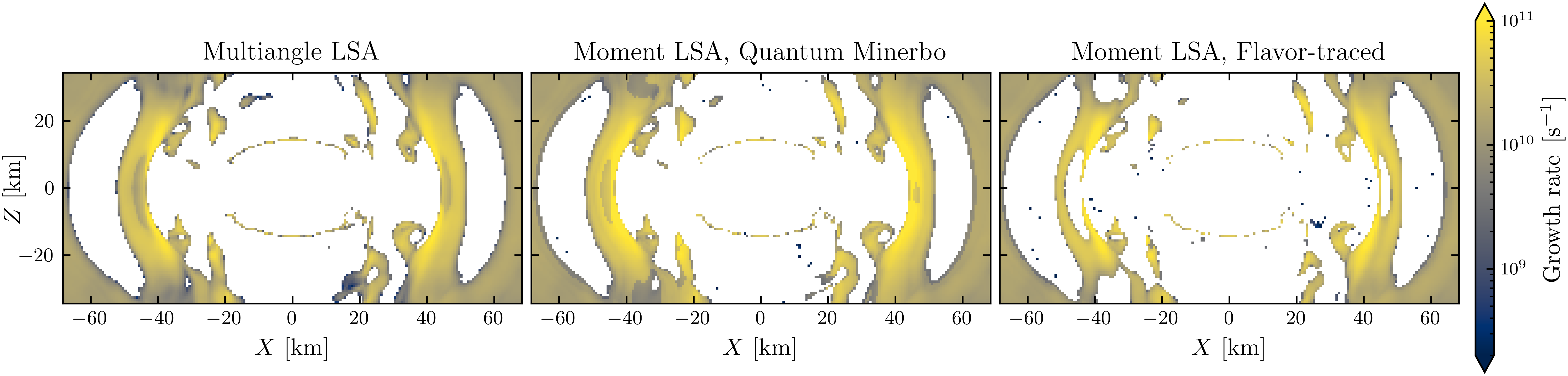
Figure 1: Predicted growth rate of FFIs in a transverse slice of the 5 ms post-merger snapshot for the M1 simulation in [58], obtained with multiangle LSA [left], two-moment LSA with the quantum closure (16) [center], and two-moment LSA with the “flavor-traced” closure (24) [right].

The results of our calculations are shown on Fig. 1. Overall, as evidenced in [39], the flavor-traced closure shows good performance in identifying the locations and characteristics of FFIs. However, one can identify several “missing regions,” where the procedure was unable to find the actual instability. On the other hand, the results with the quantum Minerbo closure identify almost perfectly the regions of instability. Generally speaking, moment methods have more difficulty in shallow crossing regions, where the precise choice of closure is of prime importance: we show here the promising features of our new closure prescriptions, with a detailed study of the impact of closure choices in various crossing landscapes left for future work.

Prospects— In this paper we have derived the first quantum generalization of an analytic closure for moment neutrino transport using the maximum entropy principle in the small flavor coherence limit. We confirmed that it approaches the correct behavior in the free-streaming and isotropic limits, and that it respects causality. Beyond the theoretical appeal of such a model, we showed the significantly better capability of this closure in correctly identifying the occurrence of FFIs in a neutron star merger, a requirement for the generalized use of quantum moment methods. We thus showed a close resemblance of the results of moment LSA using the quantum Minerbo closure compared to the multiangle LSA (Fig. 1), an improvement over alternative, ad hoc, closures used previously. Moreover, a recent study [59] suggests that, in an actual environment, neutrinos may never venture far from stability, in which case the approximation of small flavor coherence that we took in this work is well-motivated. As the first example of a quantum closure based on first principles, this work opens the way to more complex closures, and represents an important step towards the development of robust quantum moment methods for neutrino transport.

Acknowledgments— We thank E. Grohs, S. Richers and F. Foucart for many useful discussions and for comments on the manuscript, and in particular F. Foucart for providing the NSM simulation data. J.F. is supported by the Network for Neutrinos, Nuclear Astrophysics and Symmetries (N3AS), through the National Science Foundation Physics Frontier Center award No. PHY-2020275. J.P.K and G.C.M are supported by the United States Department of Energy, Office of Science, Office of Nuclear Physics (award number DE-FG02-02ER41216).

Supplemental Material for

Quantum Maximum Entropy Closure for Small Flavor Coherence

Julien Froustey ,^1,2, James P. Kneller ,² and Gail C. McLaughlin ²

¹Department of Physics, University of California Berkeley, Berkeley, CA 94720, USA

²Department of Physics, North Carolina State University, Raleigh, NC 27695, USA

We provide material that is not needed to understand the primary message of our work, including some detailed derivations and/or numerical analyses of some points introduced in the main text.

Appendix A Quantum Fermi-Dirac Maximum Entropy Closure

We derive here the fermionic version of our quantum maximum entropy closure, first derived in the classical case in [13].

Taking into account the fermionic nature of neutrinos, the functional (4) becomes:

$$\mathsf{S}[\varrho]=\int_{-1}^{1}{\mathrm{d}\mu\,\mathrm{Tr}\left[\varrho\ln(\varrho)+(\mathbb{I}-\varrho)\ln(\mathbb{I}-\varrho)\right]}-\left\langle\alpha,\int_{-1}^{1}{\mathrm{d}\mu\varrho}-\frac{N}{2\pi\varrho_{0}}\right\rangle-\left\langle Z,\int_{-1}^{1}{\mathrm{d}\mu\mu\varrho}-\frac{F^{z}}{2\pi\varrho_{0}}\right\rangle\,,$$ (S.1)

where $\varrho_{0}$ is a normalization factor, needed to ensure that $\varrho_{aa}$ is a distribution function with $0\leq\varrho_{aa}\leq 1$.

The additional term compared to the Maxwell-Boltzmann limit (4) gives a contribution identical to (11) with $\varrho_{aa}\to 1-\varrho_{aa}$, that is,

$$\mathrm{Tr}\left[(\mathbb{I}-\varrho)\ln(\mathbb{I}-\varrho)\right]=(1-\varrho_{ee})\ln(1-\varrho_{ee})+(1-\varrho_{xx})\ln(1-\varrho_{xx})-\frac{\ln(1-\varrho_{ee})-\ln(1-\varrho_{xx})}{\varrho_{ee}-\varrho_{xx}}\lvert\varrho_{ex}\rvert^{2}+\cdots$$ (S.2)

For completeness, we quote the same formulae, but written for any number of flavors:

$$\mathrm{Tr}\left[\varrho\ln(\varrho)\right] =\sum_{a}{\varrho_{aa}\ln(\varrho_{aa})}+\frac{1}{2}\sum_{a\neq b}{\frac{\ln(\varrho_{aa})-\ln(\varrho_{bb})}{\varrho_{aa}-\varrho_{bb}}\lvert\varrho_{ab}\rvert^{2}}+\cdots\,,$$ (S.3)

$$\mathrm{Tr}\left[(\mathbb{I}-\varrho)\ln(\mathbb{I}-\varrho)\right] =\sum_{a}{(1-\varrho_{aa})\ln(1-\varrho_{aa})}-\frac{1}{2}\sum_{a\neq b}{\frac{\ln(1-\varrho_{aa})-\ln(1-\varrho_{bb})}{\varrho_{aa}-\varrho_{bb}}\lvert\varrho_{ab}\rvert^{2}}+\cdots\,.$$ (S.4)

Flavor-diagonal elements —

Maximizing (S.1) over $\varrho_{aa}$ leads at leading order to:

$$\ln(\varrho_{aa})-\ln(1-\varrho_{aa})-\alpha_{aa}\varrho_{aa}-Z_{aa}\mu\varrho_{aa}=0\,,$$ (S.5)

such that

$$\frac{\varrho_{aa}}{1-\varrho_{aa}}=e^{\alpha_{aa}}e^{Z_{aa}\mu}\ ,\qquad\text{or equivalently}\qquad\varrho_{aa}=\frac{1}{e^{-\alpha_{aa}}e^{-Z_{aa}\mu}+1}\,.$$ (S.6)

The constraints read:

$$2\pi\int_{-1}^{1}{\mathrm{d}\mu\begin{bmatrix}1\\ \mu\end{bmatrix}\frac{\varrho_{0}}{e^{-\alpha_{aa}}e^{-Z_{aa}\mu}+1}}=\begin{bmatrix}N_{aa}\\ F_{aa}^{z}\end{bmatrix}\,.$$ (S.7)

They were historically numerically inverted or considered in a Padé approximation, before Cernohorsky and Bludman [14] found an approximate closed-form for the Eddington factor $P_{aa}^{zz}/N_{aa}$ (see also [9, 10]).

Flavor off-diagonal elements —

We now maximize (S.1) with respect to $\mathrm{Re}(\varrho_{ex})$ and $\mathrm{Im}(\varrho_{ex})$. The result is straightforward given the Maxwell-Boltzmann derivation in the main text, as the term in $\mathsf{S}[\varrho]$ involving $\varrho_{ex}$ that changes because of Fermi-Dirac statistics reads:

$$\mathsf{S}[\varrho]\supset\frac{\ln\left(\dfrac{\varrho_{ee}}{1-\varrho_{ee}}\right)-\ln\left(\dfrac{\varrho_{xx}}{1-\varrho_{xx}}\right)}{\varrho_{ee}-\varrho_{xx}}\left\lvert\varrho_{ex}\right\rvert^{2}\,,$$ (S.8)

such that Eq. (13) becomes:

$$\varrho_{ex}(\mu)=\frac{\varrho_{ee}-\varrho_{xx}}{\ln\left(\dfrac{\varrho_{ee}}{1-\varrho_{ee}}\right)-\ln\left(\dfrac{\varrho_{xx}}{1-\varrho_{xx}}\right)}\left(\alpha_{ex}+\mu Z_{ex}\right)\,.$$ (S.9)

Therefore, Eqs. (15)–(17) keep the same form, where the $I_{(n)}$ integrals are modified via $\varrho_{aa}\to\varrho_{aa}/(1-\varrho_{aa})$ inside the logarithms. Notably, the angular dependence of the denominator of $I_{(n)}$ remains linear in $\mu$, just like in the Maxwell-Boltzmann case.

Appendix B Closure Parameters in the Free-Streaming Regime

In this section, we provide a derivation of the limits of the closure coefficients $\kappa$ and $\eta$ when the flux factors for $\nu_{e}$ and $\nu_{x}$ approach $1$.

When $f_{ee}\to 1$, $Z_{ee}\to+\infty$ according to Eq. (3), such that $\varrho_{ee}(\mu)\sim(N_{ee}/2\pi)Z_{ee}e^{Z_{ee}(\mu-1)}$. This is a function that, for $Z_{ee}\to+\infty$, is non-zero only in a small neighborhood of $\mu=1$. The same arguments apply to $\varrho_{xx}$. Recalling that

$$I_{(n)}=2\pi\int_{-1}^{1}{\mathrm{d}\mu\,\mu^{n}\frac{\varrho_{ee}-\varrho_{xx}}{\ln(\varrho_{ee})-\ln(\varrho_{xx})}}\equiv 2\pi\int_{-1}^{1}{\mathrm{d}\mu\,\mu^{n}\,h(\mu)}\,,$$ (S.10)

we distinguish different cases.

First, if $\varrho_{ee}(\mu)=\varrho_{xx}(\mu)$, since the limit of $x\mapsto(x-1)/\ln(x)$ for $x\to 1$ is $1$, then $h(\mu)=\varrho_{ee}(\mu)$.

Otherwise, we have $N_{ee}\neq N_{xx}$ and/or $Z_{ee}\neq Z_{xx}$, such that the denominator of $h(\mu)$ reads, in the $f_{aa}\to 1$ limit, $\ln(N_{ee}/N_{xx})+(Z_{ee}-Z_{xx})\mu$, which is a slowly varying function of $\mu$ compared to the exponentials in the numerator. Since the support of $I_{(n)}$ is very localized at $\mu\lesssim 1$, we can take the denominator as constant. Assuming, without loss of generality, that $Z_{xx}>Z_{ee}\gg 1$, we have

$$\varrho_{ee}-\varrho_{xx}=\varrho_{ee}\left(1-\frac{\varrho_{xx}}{\varrho_{ee}}\right)\sim\varrho_{ee}\,,$$ (S.11)

as $\forall\mu<1$, $\varrho_{xx}/\varrho_{ee}\sim(N_{ee}Z_{ee}/N_{xx}Z_{xx})e^{-(Z_{xx}-Z_{ee})(1-\mu)}\ll 1$.

Consequently, in any case, $I_{(n)}$ is given, in the free-streaming limit, by $I_{(n)}=C\times J_{(n)}(1/Z_{ee})$, with $C$ a constant independent of $n$, and

$$J_{(n)}(\varepsilon)\equiv\int_{-1}^{1}{\mathrm{d}\mu\,\mu^{n}\frac{1/\varepsilon}{2\sinh(1/\varepsilon)}e^{\mu/\varepsilon}}\,.$$ (S.12)

In particular, this means that the limits of $\kappa$ and $\eta$, defined by Eq. (17), are given by:

$$\lim_{f_{ee},f_{xx}\to 1}\kappa=\lim_{\varepsilon\to 0}\frac{J_{(2)}^{2}-J_{(1)}J_{(3)}}{J_{(0)}J_{(2)}-J_{(1)}^{2}}\ ,\qquad\quad\lim_{f_{ee},f_{xx}\to 1}\eta=\lim_{\varepsilon\to 0}\frac{J_{(0)}J_{(3)}-J_{(1)}J_{(2)}}{J_{(0)}J_{(2)}-J_{(1)}^{2}}\,.$$ (S.13)

We have, for $Z_{ee}\to\infty$ and thus $\varepsilon\to 0$,

$$J_{(0)} =1\,,\quad \quad J_{(2)} \sim 1-2\varepsilon+2\varepsilon^{2}\,,$$ (S.14)

$$J_{(1)} \sim 1-\varepsilon\,,\quad \quad J_{(3)} \sim 1-3\varepsilon+6\varepsilon^{2}-6\varepsilon^{3}\,.$$

As a consequence,

$$J_{(0)}J_{(2)}-J_{(1)}^{2} \sim\varepsilon^{2}\,,$$ (S.15)

$$J_{(2)}^{2}-J_{(1)}J_{(3)} \sim-\varepsilon^{2}\,,$$

$$J_{(0)}J_{(3)}-J_{(1)}J_{(2)} \sim 2\varepsilon^{2}\,.$$

Inserting those asymptotic equivalents in Eq. (S.13), we proved that $\kappa\to-1$ and $\eta\to 2$. If the flux factors tend to $-1$, the support of $J_{(n)}$ is around $-1$ and there is an extra minus sign in front of all the odd $J_{(n)}$, such that $\eta\to-2$.

Appendix C Numerical Study of $\lambda_{ex}^{(\pm)}$

In order to verify that the additional characteristic speeds (23) satisfy the causality requirements $\lvert\lambda_{ex}^{(\pm)}\rvert\leq 1$, we perform a numerical scan over the parameter space that can be spanned by the Minerbo distributions entering Eq. (17).

First, assuming without loss of generality that $N_{ee}\geq N_{xx}$, we rewrite the $I_{(n)}$ integrals as:

$$I_{(n)}=\frac{N_{xx}}{2}\int_{-1}^{1}{\mathrm{d}{\mu}\,\mu^{n}\frac{\widetilde{N}\dfrac{Z_{ee}}{\sinh(Z_{ee})}e^{Z_{ee}\mu}-\dfrac{Z_{xx}}{\sinh(Z_{xx})}e^{Z_{xx}\mu}}{\ln\left[\widetilde{N}\dfrac{Z_{ee}\sinh(Z_{xx})}{Z_{xx}\sinh(Z_{ee})}\right]+(Z_{ee}-Z_{xx})\mu}}\,,$$ (S.16)

with $\widetilde{N}=N_{ee}/N_{xx}$. Since ratios of $I_{(n)}$ appear in the functions $\kappa$ and $\eta$, these quantities (and the related characteristic speeds $\lambda_{ex}^{(\pm)}$) are functions of three parameters: $\widetilde{N}\in[1,+\infty)$, $Z_{ee}\in\mathbb{R}$, and $Z_{xx}\in\mathbb{R}$ (note that a negative $Z_{aa}$ corresponds to $F_{aa}^{z}\leq 0$). We plot in Fig. A the maximum quantum characteristic speed, scanning over the parameter ranges. When $\lvert Z_{aa}\rvert\gg 1$, meaning that $\nu_{a}$ is free-streaming, the maximum characteristic speed goes to $1$, as expected by causality requirements [51]. When both $\lvert Z_{ee}\rvert,\lvert Z_{xx}\rvert\ll 1$, this is the isotropic limit for which $\eta\to 0$ and $\kappa\to 1/3$, so that $\lvert\lambda_{ex}^{(\pm)}\rvert\to 1/\sqrt{3}\simeq 0.577$.

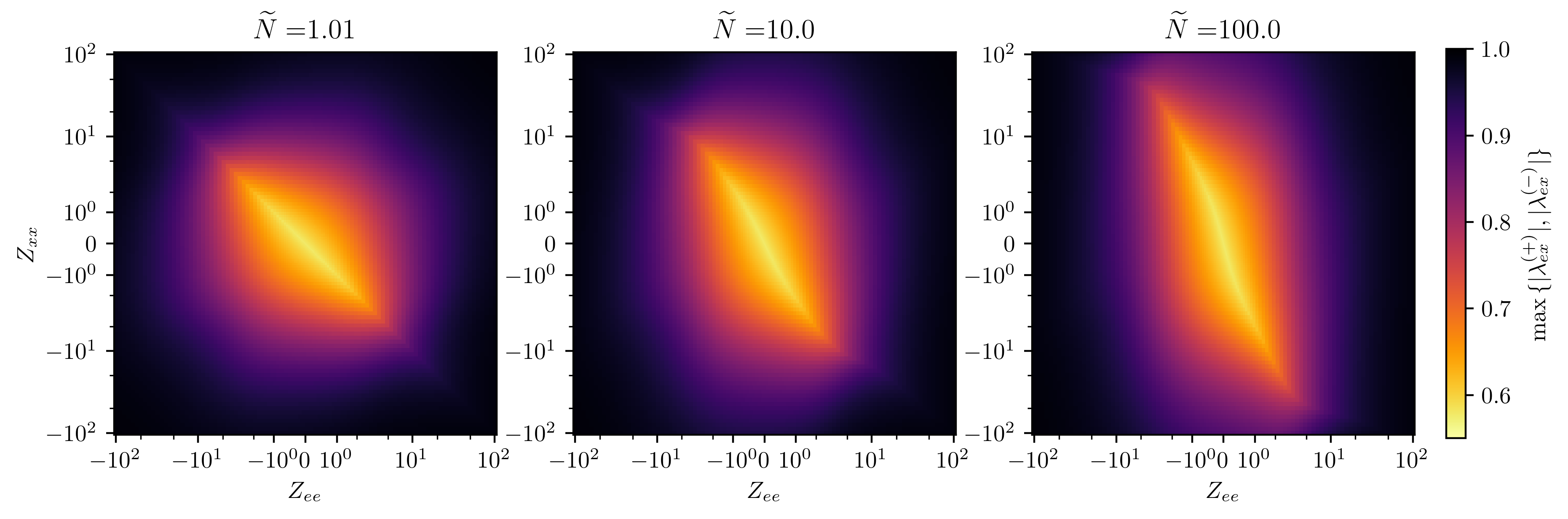
Figure A: Maximum $\lambda_{ex}$ characteristic speed across the range of values of $\{Z_{ee},Z_{xx}\}$, for three relative number densities $\widetilde{N}\in\{1.01,10,100\}$.

We thus explicitly show that characteristic speeds are everywhere physical, an important requirement for a closure to be used in large-scale hydrodynamic simulations.

As an additional illustration, we show on Fig. B the largest quantum characteristic speed at each point in the transverse slice of the 5 ms post-merger snapshot from [58], studied in the main text (see Fig. 1). As proved above, the characteristic speeds are always below unity, approaching the isotropic limit in the center of the slice ($\lambda_{ex}^{(\pm)}\to\pm 1/\sqrt{3}\simeq 0.577$). The characteristic speeds do not get significantly close to $1$ in this snapshot, as the simulation box is rather close to the remnant.

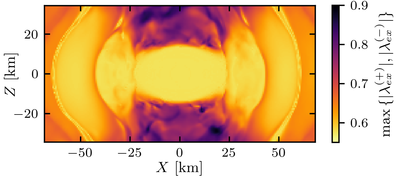
Figure B: Largest characteristic speed $\lvert\lambda_{ex}^{(\pm)}\rvert$ in a transverse slice of the 5 ms post-merger snapshot from the NSM simulation [58].

References

- Mezzacappa et al. [2020] A. Mezzacappa, E. Endeve, O. E. Bronson Messer, and S. W. Bruenn, Physical, numerical, and computational challenges of modeling neutrino transport in core-collapse supernovae, Liv. Rev. Comput. Astrophys. 6, 4 (2020), arXiv:2010.09013 [astro-ph.HE] .
- Foucart [2023] F. Foucart, Neutrino transport in general relativistic neutron star merger simulations, Liv. Rev. Comput. Astrophys. 9, 1 (2023), arXiv:2209.02538 [astro-ph.HE] .
- Fischer et al. [2024] T. Fischer, G. Guo, K. Langanke, G. Martinez-Pinedo, Y.-Z. Qian, and M.-R. Wu, Neutrinos and nucleosynthesis of elements, Prog. Part. Nucl. Phys. 137, 104107 (2024), arXiv:2308.03962 [astro-ph.HE] .
- Wang and Surman [2023] X. Wang and R. Surman, Neutrinos and Heavy Element Nucleosynthesis, in Handbook of Nuclear Physics, edited by I. Tanihata, H. Toki, and T. Kajino (Springer Nature Singapore, Singapore, 2023) pp. 1–19, arXiv:2309.06043 [astro-ph.HE] .
- Thorne [1981] K. S. Thorne, Relativistic radiative transfer: moment formalisms, Mon. Not. Roy. Astron. Soc. 194, 439 (1981).
- Shibata et al. [2011] M. Shibata, K. Kiuchi, Y.-i. Sekiguchi, and Y. Suwa, Truncated Moment Formalism for Radiation Hydrodynamics in Numerical Relativity, Prog. Theor. Phys. 125, 1255 (2011), arXiv:1104.3937 [astro-ph.HE] .
- Cardall et al. [2013] C. Y. Cardall, E. Endeve, and A. Mezzacappa, Conservative 3+1 General Relativistic Variable Eddington Tensor Radiation Transport Equations, Phys. Rev. D 87, 103004 (2013), arXiv:1209.2151 [astro-ph.HE] .
- Levermore [1984] C. D. Levermore, Relating Eddington factors to flux limiters, J. Quant. Spectrosc. Radiat. Transfer 31, 149 (1984).
- Smit et al. [2000] J. M. Smit, L. J. van den Horn, and S. A. Bludman, Closure in flux-limited neutrino diffusion and two-moment transport, Astron. Astrophys. 356, 559 (2000).
- Murchikova et al. [2017] L. M. Murchikova, E. Abdikamalov, and T. Urbatsch, Analytic Closures for M1 Neutrino Transport, Mon. Not. Roy. Astron. Soc. 469, 1725 (2017), arXiv:1701.07027 [astro-ph.HE] .
- Richers [2020] S. Richers, Rank-3 Moment Closures in General Relativistic Neutrino Transport, Phys. Rev. D 102, 083017 (2020), arXiv:2009.09046 [astro-ph.HE] .
- Minerbo [1978] G. N. Minerbo, Maximum entropy Eddington factors., J. Quant. Spectrosc. Radiat. Transfer 20, 541 (1978).
- Cernohorsky et al. [1989] J. Cernohorsky, L. J. van den Horn, and J. Cooperstein, Maximum entropy Eddington factors in flux-limited neutrino diffusion., J. Quant. Spectrosc. Radiat. Transfer 42, 603 (1989).
- Cernohorsky and Bludman [1994] J. Cernohorsky and S. A. Bludman, Maximum Entropy Distribution and Closure for Bose-Einstein and Fermi-Dirac Radiation Transport, Astrophys. J. 433, 250 (1994).
- Wolfenstein [1978] L. Wolfenstein, Neutrino Oscillations in Matter, Phys. Rev. D 17, 2369 (1978).
- Mikheyev and Smirnov [1985] S. P. Mikheyev and A. Y. Smirnov, Resonant Amplification of Oscillations in Matter and Spectroscopy of Solar Neutrinos, Sov. J. Nucl. Phys. 42, 913 (1985).
- Loreti et al. [1995] F. N. Loreti, Y. Z. Qian, G. M. Fuller, and A. B. Balantekin, Effects of random density fluctuations on matter enhanced neutrino flavor transitions in supernovae and implications for supernova dynamics and nucleosynthesis, Phys. Rev. D 52, 6664 (1995), arXiv:astro-ph/9508106 .
- Kneller and Volpe [2010] J. P. Kneller and C. Volpe, Turbulence effects on supernova neutrinos, Phys. Rev. D 82, 123004 (2010), arXiv:1006.0913 [hep-ph] .
- Duan et al. [2010] H. Duan, G. M. Fuller, and Y.-Z. Qian, Collective Neutrino Oscillations, Ann. Rev. Nucl. Part. Sci. 60, 569 (2010), arXiv:1001.2799 [hep-ph] .
- Malkus et al. [2012] A. Malkus, J. P. Kneller, G. C. McLaughlin, and R. Surman, Neutrino oscillations above black hole accretion disks: disks with electron-flavor emission, Phys. Rev. D 86, 085015 (2012), arXiv:1207.6648 [hep-ph] .
- Wu et al. [2016] M.-R. Wu, H. Duan, and Y.-Z. Qian, Physics of neutrino flavor transformation through matter–neutrino resonances, Phys. Lett. B 752, 89 (2016), arXiv:1509.08975 [hep-ph] .
- Horiuchi and Kneller [2018] S. Horiuchi and J. P. Kneller, What can be learned from a future supernova neutrino detection?, J. Phys. G 45, 043002 (2018), arXiv:1709.01515 [astro-ph.HE] .
- Tamborra and Shalgar [2021] I. Tamborra and S. Shalgar, New Developments in Flavor Evolution of a Dense Neutrino Gas, Ann. Rev. Nucl. Part. Sci. 71, 165 (2021), arXiv:2011.01948 [astro-ph.HE] .
- Johns [2023] L. Johns, Collisional Flavor Instabilities of Supernova Neutrinos, Phys. Rev. Lett. 130, 191001 (2023), arXiv:2104.11369 [hep-ph] .
- Capozzi and Saviano [2022] F. Capozzi and N. Saviano, Neutrino Flavor Conversions in High-Density Astrophysical and Cosmological Environments, Universe 8, 94 (2022), arXiv:2202.02494 [hep-ph] .
- Richers and Sen [2022] S. Richers and M. Sen, Fast Flavor Transformations, in Handbook of Nuclear Physics, edited by I. Tanihata, H. Toki, and T. Kajino (Springer Nature Singapore, Singapore, 2022) pp. 1–17, arXiv:2207.03561 [astro-ph.HE] .
- Volpe [2024] M. C. Volpe, Neutrinos from dense environments: Flavor mechanisms, theoretical approaches, observations, and new directions, Rev. Mod. Phys. 96, 025004 (2024), arXiv:2301.11814 [hep-ph] .
- Sen [2024] M. Sen, Supernova Neutrinos: Flavour Conversion Mechanisms and New Physics Scenarios, Universe 10, 238 (2024), arXiv:2405.20432 [hep-ph] .
- Stapleford et al. [2020] C. J. Stapleford, C. Fröhlich, and J. P. Kneller, Coupling neutrino oscillations and simulations of core-collapse supernovae, Phys. Rev. D 102, 081301 (2020), arXiv:1910.04172 [astro-ph.HE] .
- Li and Siegel [2021] X. Li and D. M. Siegel, Neutrino Fast Flavor Conversions in Neutron-Star Postmerger Accretion Disks, Phys. Rev. Lett. 126, 251101 (2021), arXiv:2103.02616 [astro-ph.HE] .
- Just et al. [2022] O. Just, S. Abbar, M.-R. Wu, I. Tamborra, H.-T. Janka, and F. Capozzi, Fast neutrino conversion in hydrodynamic simulations of neutrino-cooled accretion disks, Phys. Rev. D 105, 083024 (2022), arXiv:2203.16559 [astro-ph.HE] .
- Ehring et al. [2023a] J. Ehring, S. Abbar, H.-T. Janka, G. Raffelt, and I. Tamborra, Fast neutrino flavor conversion in core-collapse supernovae: A parametric study in 1D models, Phys. Rev. D 107, 103034 (2023a), arXiv:2301.11938 [astro-ph.HE] .
- Ehring et al. [2023b] J. Ehring, S. Abbar, H.-T. Janka, G. Raffelt, and I. Tamborra, Fast Neutrino Flavor Conversions Can Help and Hinder Neutrino-Driven Explosions, Phys. Rev. Lett. 131, 061401 (2023b), arXiv:2305.11207 [astro-ph.HE] .
- Johns et al. [2020a] L. Johns, H. Nagakura, G. M. Fuller, and A. Burrows, Neutrino oscillations in supernovae: angular moments and fast instabilities, Phys. Rev. D 101, 043009 (2020a), arXiv:1910.05682 [hep-ph] .
- Johns et al. [2020b] L. Johns, H. Nagakura, G. M. Fuller, and A. Burrows, Fast oscillations, collisionless relaxation, and spurious evolution of supernova neutrino flavor, Phys. Rev. D 102, 103017 (2020b), arXiv:2009.09024 [hep-ph] .
- Myers et al. [2022] M. Myers, T. Cooper, M. Warren, J. Kneller, G. McLaughlin, S. Richers, E. Grohs, and C. Frohlich, Neutrino flavor mixing with moments, Phys. Rev. D 105, 123036 (2022), arXiv:2111.13722 [hep-ph] .
- Grohs et al. [2023] E. Grohs, S. Richers, S. M. Couch, F. Foucart, J. P. Kneller, and G. C. McLaughlin, Neutrino fast flavor instability in three dimensions for a neutron star merger, Phys. Lett. B 846, 138210 (2023), arXiv:2207.02214 [hep-ph] .
- Grohs et al. [2024] E. Grohs, S. Richers, S. M. Couch, F. Foucart, J. Froustey, J. P. Kneller, and G. C. McLaughlin, Two-moment Neutrino Flavor Transformation with Applications to the Fast Flavor Instability in Neutron Star Mergers, Astrophys. J. 963, 11 (2024), arXiv:2309.00972 [astro-ph.HE] .
- Froustey et al. [2024] J. Froustey, S. Richers, E. Grohs, S. D. Flynn, F. Foucart, J. P. Kneller, and G. C. McLaughlin, Neutrino fast flavor oscillations with moments: Linear stability analysis and application to neutron star mergers, Phys. Rev. D 109, 043046 (2024), arXiv:2311.11968 [astro-ph.HE] .
- Padilla-Gay et al. [2021] I. Padilla-Gay, S. Shalgar, and I. Tamborra, Multi-Dimensional Solution of Fast Neutrino Conversions in Binary Neutron Star Merger Remnants, JCAP 01, 017, arXiv:2009.01843 [astro-ph.HE] .
- Richers et al. [2022] S. Richers, H. Duan, M.-R. Wu, S. Bhattacharyya, M. Zaizen, M. George, C.-Y. Lin, and Z. Xiong, Code comparison for fast flavor instability simulations, Phys. Rev. D 106, 043011 (2022), arXiv:2205.06282 [astro-ph.HE] .
- Nagakura [2022] H. Nagakura, General-relativistic quantum-kinetics neutrino transport, Phys. Rev. D 106, 063011 (2022), arXiv:2206.04098 [astro-ph.HE] .
- Nagakura and Zaizen [2023] H. Nagakura and M. Zaizen, Basic characteristics of neutrino flavor conversions in the postshock regions of core-collapse supernova, Phys. Rev. D 108, 123003 (2023), arXiv:2308.14800 [astro-ph.HE] .
- Xiong et al. [2024] Z. Xiong, M.-R. Wu, M. George, C.-Y. Lin, N. K. Largani, T. Fischer, and G. Martinez-Pinedo, Fast neutrino flavor conversions in a supernova: Emergence, evolution, and effects, Phys. Rev. D 109, 123008 (2024), arXiv:2402.19252 [astro-ph.HE] .
- Richers et al. [2024] S. Richers, J. Froustey, S. Ghosh, F. Foucart, and J. Gomez, Asymptotic-state prediction for fast flavor transformation in neutron star mergers, arXiv:2409.04405 [astro-ph.HE] (2024).
- Sigl and Raffelt [1993] G. Sigl and G. Raffelt, General kinetic description of relativistic mixed neutrinos, Nucl. Phys. B 406, 423 (1993).
- Volpe et al. [2013] C. Volpe, D. Väänänen, and C. Espinoza, Extended evolution equations for neutrino propagation in astrophysical and cosmological environments, Phys. Rev. D 87, 113010 (2013), arXiv:1302.2374 [hep-ph] .
- Vlasenko et al. [2014] A. Vlasenko, G. M. Fuller, and V. Cirigliano, Neutrino Quantum Kinetics, Phys. Rev. D 89, 105004 (2014), arXiv:1309.2628 [hep-ph] .
- [49] S. L. Adler, Taylor expansion and derivate formulas for matrix logarithms, https://www.ias.edu/sites/default/files/sns/files/1-matrixlog_tex.pdf.
- Haber [2023] H. E. Haber, Notes on the matrix exponential and logarithm, https://scipp.ucsc.edu/~haber/webpage/MatrixExpLog.pdf (2023).
- Anile et al. [1991] A. M. Anile, S. Pennisi, and M. Sammartino, A thermodynamical approach to Eddington factors, J. Math. Phys. 32, 544 (1991).
- Liu et al. [2023] J. Liu, M. Zaizen, and S. Yamada, Systematic study of the resonancelike structure in the collisional flavor instability of neutrinos, Phys. Rev. D 107, 123011 (2023), arXiv:2302.06263 [hep-ph] .
- Patwardhan et al. [2023] A. V. Patwardhan, M. J. Cervia, E. Rrapaj, P. Siwach, and A. B. Balantekin, Many-Body Collective Neutrino Oscillations: Recent Developments, in Handbook of Nuclear Physics, edited by I. Tanihata, H. Toki, and T. Kajino (2023) pp. 1–16, arXiv:2301.00342 [hep-ph] .
- Richers et al. [2019] S. A. Richers, G. C. McLaughlin, J. P. Kneller, and A. Vlasenko, Neutrino Quantum Kinetics in Compact Objects, Phys. Rev. D 99, 123014 (2019), [Erratum: Phys. Rev. D 109, 129902 (2024)], arXiv:1903.00022 [astro-ph.HE] .
- Audit et al. [2002] E. Audit, P. Charrier, J. P. Chieze, and B. Dubroca, A radiation-hydrodynamics scheme valid from the transport to the diffusion limit, arXiv:astro-ph/0206281 (2002).
- Morinaga [2022] T. Morinaga, Fast neutrino flavor instability and neutrino flavor lepton number crossings, Phys. Rev. D 105, L101301 (2022), arXiv:2103.15267 [hep-ph] .
- Dasgupta [2022] B. Dasgupta, Collective Neutrino Flavor Instability Requires a Crossing, Phys. Rev. Lett. 128, 081102 (2022), arXiv:2110.00192 [hep-ph] .
- Foucart et al. [2016] F. Foucart, E. O’Connor, L. Roberts, L. E. Kidder, H. P. Pfeiffer, and M. A. Scheel, Impact of an improved neutrino energy estimate on outflows in neutron star merger simulations, Phys. Rev. D 94, 123016 (2016), arXiv:1607.07450 [astro-ph.HE] .
- Fiorillo and Raffelt [2024] D. F. G. Fiorillo and G. Raffelt, Fast flavor conversions at the edge of instability, arXiv:2403.12189 [hep-ph] (2024).