Sample-Efficient Bayesian Optimization with Transfer Learning for Heterogeneous Search Spaces

Abstract

Bayesian optimization (BO) is a powerful approach to sample-efficient optimization of black-box functions. However, in settings with very few function evaluations, a successful application of BO may require transferring information from historical experiments. These related experiments may not have exactly the same tunable parameters (search spaces), motivating the need for BO with transfer learning for heterogeneous search spaces. In this paper, we propose two methods for this setting. The first approach leverages a Gaussian process (GP) model with a conditional kernel to transfer information between different search spaces. Our second approach treats the missing parameters as hyperparameters of the GP model that can be inferred jointly with the other GP hyperparameters or set to fixed values. We show that these two methods perform well on several benchmark problems.

1  Introduction

Bayesian optimization (BO) is a popular technique for sample-efficient black-box optimization that has been successfully leveraged for a wide range of applications such as hyperparameter tuning for machine learning models (Turner et al., 2021; Snoek et al., 2012), A/B testing (Letham et al., 2019), chemical engineering (Hernández-Lobato et al., 2017), materials science (Ueno et al., 2016), control systems (Candelieri et al., 2018), and drug discovery (Negoescu et al., 2011). Many approaches to BO target the setting of expensive black-box functions where we only have access to a small number of function evaluations. To further improve the performance of BO in this setting, transfer learning can be used as a way of leveraging relevant historical information. While transfer learning has been thoroughly studied in the BO literature, traditional transfer learning approaches typically assume that all related experiments have exactly the same (homogeneous) search space. This assumption simplifies the modeling process, but significantly limits the applicability of these methods in real-world scenarios where search spaces often vary between experiments. For instance, when tuning the hyperparameters of machine learning models, practitioners often make changes to the search space to add and/or remove parameters or update their ranges.

In this regime, we need a BO method that can seamlessly transfer information from several historical experiments with different search spaces. To achieve this, we propose two methods targeting the setting of a small number of function evaluations where we do not have access to additional domain knowledge, e.g., user priors. Our first method leverages a conditional kernel that defines a similarity measure between heterogeneous spaces by leveraging a tree-structured representation of the search spaces. This method has the advantage that it requires no additional hyperparameters. Our second method employs a learned imputation which treats missing parameters as hyperparameters that can be learned jointly with the other GP hyperparameters. Both methods allow incorporating task-level similarity information and naturally correspond to standard transfer learning BO in the special case when the search spaces are identical. Our main contributions are:

1. We propose two methods (conditional kernel-based and learned imputation-based) for BO with transfer learning for heterogeneous search spaces.

2. We empirically validate our methods on benchmark datasets, demonstrating better sample-efficiency compared to existing approaches.

3. We provide a BoTorch implementations of both approaches.

2  Related Work

Transfer Learning in Bayesian Optimization (BO)

BO has been previously explored with the common goal of leveraging information from historical source tasks to improve optimization efficiency on a new target task (Bai et al., 2023). Early work by (Swersky et al., 2013; Yogatama and Mann, 2014)) employed multi-task Gaussian Processes (MTGPs) to model task similarities. In addition, (Tighineanu et al., 2022) provide a unified view of hierarchical GP models for transfer learning in BO. Ensemble methods have also been utilized as surrogate models in the context of transfer learning (Schilling et al., 2016; Feurer et al., 2018).

Recent work has also considered learning neural network-parameterized GP priors from previous tasks (Perrone et al., 2018; Wistuba and Grabocka, 2021; Wang et al., 2021). Additionally, (Shilton et al., 2017; Wang et al., 2018; Dai et al., 2022) performed a theoretical analysis for the regret metric commonly employed in BO. However, all these approaches focus on the setting where the search spaces are homogeneous across tasks, i.e., all tasks share the same search space. This limits these methods applicability for problems with different (heterogeneous) search spaces.

BO with Heterogeneous Search Spaces

(Fan et al., 2024) recently proposed a method for transfer learning across heterogeneous search spaces that leverages a neural network mapping from domain-specific contexts to specifications of hierarchical GPs. The data requirements of neural networks and the need for manually defined domain-specific contexts may limit the applicability of this method in settings where small amounts of data is available. Another class of recent methods leverage text-based sequential modeling approaches for meta black-box optimization (Chen et al., 2022; Song et al., 2024). While this sequential modeling can naturally handle heterogeneous search spaces, these methods require massive amounts of training data. During paper review, we became aware of (Stoll et al., 2020), which motivates the heterogeneity through the adjustments made across a sequence of hyperparameter optimizations for machine learning models. They introduce the problem, a series of benchmark problems and baseline algorithms; and demonstrate that transferring knowledge across experiments can lead to significant savings in experimentation budget.

3  Background

Bayesian Optimization

Bayesian optimization (BO) is an iterative approach to black-box optimization, see (Frazier, 2018; Garnett, 2023) for a comprehensive overview. BO consists of two main steps where we first build a probabilistic surrogate model from available data followed by optimizing an acquisition function to select the most promising candidate(s) to evaluate next. This iterative process continues until the evaluation budget has been exhausted. The probabilistic surrogate model is commonly a Gaussian process (GP) (Rasmussen et al., 2006) and a common choice of acquisition function is the expected improvement (EI) (Jones et al., 1998).

Bayesian Optimization with Transfer Learning

Our goal is to optimize a target black-box function (task) $f_{t}(x)$ where each evaluation of $f_{t}(x)$ is expensive and the number of function evaluations is limited. We assume a budget of $n$ function evaluations for $f_{t}(x)$, where $n$ is commonly between $5$ and $40$. In the transfer learning setting we are also given data from a set of $t-1$ related optimization experiments, referred to as source tasks, $f_{1},f_{2},\ldots,f_{t-1}$. We want to leverage this existing data to improve the sample-efficiency of BO on the target task $f_{t}(x)$.

In this paper, we are interested in the setting where tasks are heterogeneous, i.e., correspond to different search spaces. As an example, consider tuning a few hyperparameters of a simple neural network with source tasks $f_{1}(x),f_{2}(x)$ and target task $f_{3}(x)$ with search spaces defined as follows:

• Search space of $f_{1}$: $\mathcal{X}_{1}$ = {learning rate, dropout rate}

• Search space of $f_{2}$ : $\mathcal{X}_{2}$ = {learning rate, dropout rate, batch size}

• Search space of $f_{3}$: $\mathcal{X}_{3}$ = {learning rate, dropout rate, number of hidden layers}

In this simple example, the common parameters are {learning rate, dropout ratio}, with the search spaces of $f_{2}(x)$ and $f_{3}(x)$ having some additional parameters not present in the other tasks.

4  BO with Transfer Learning for Heterogeneous Search Spaces

In this section, we will propose two methods for BO with transfer learning for heterogeneous search spaces. Our first method uses a conditional kernel which allows us to leverage a GP model to correlate the common parameters across tasks. Our second method treats the missing parameters for each task as hyperparameters that will need to be inferred when training the GP model. A clear benefit of these methods compared to existing methods in the literature, e.g., (Fan et al., 2024; Chen et al., 2022; Song et al., 2024), is that neither method assumes additional information beyond the previously evaluated inputs and corresponding function values of the source and target tasks.

4.1  MTGP with Conditional Kernels

Next, we will describe a GP model that employs a new kernel (referred as Conditional Kernel) to handle the challenge of modeling heterogeneous search spaces across different tasks. The key idea behind Conditional Kernel is to leverage a set of base kernels, e.g., Matern-5/2, to conditionally compare inputs from different tasks based on their matching parameters in a dependency tree representing the search spaces of all the tasks.

Tree-Structured Representation of Heterogeneous Search Spaces

To make this more concrete, let $\mathcal{U}=\bigcup_{i=1}^{t}\mathcal{X}_{i}$ be the universal set of parameters from all the tasks. We create a tree-representation of this universal set $\mathcal{U}$ where each node of the tree corresponds to a subset of parameters. Starting from the root node, we assign a maximal subset of parameters to each node that are common across as many tasks as possible. Subsequently, we define a set of base kernels that is equal to the number of nodes in the tree. Fig. 1 illustrates this tree for the example given in Sec. 3.

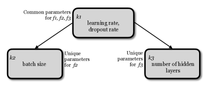
Figure 1: The tree-based representation and the corresponding kernels of the search spaces $\mathcal{X}_{1},\mathcal{X}_{2}$ and $\mathcal{X}_{3}$ given in Sec. 3.

Conditional kernel

The Conditional Kernel ($\mathcal{K}_{c}$) of any two inputs $x$ and $x^{\prime}$ coming from two tasks $i,i^{\prime}$ is defined as the sum of base kernels over all nodes that contain the common parameters across both task $i$ and task $i^{\prime}$:

$$\mathcal{K}_{c}(\{x,i\},\{x^{\prime},i^{\prime}\})=\sum_{j=1}^{p}\textbf{\text{{I}}}[N_{\mathcal{U}}[j]\subset\mathcal{X}_{i}\cap\mathcal{X}_{i^{\prime}}]\cdot k_{j}(x[N_{\mathcal{U}}[j]],x^{\prime}[N_{\mathcal{U}}[j]]),$$

where $N_{\mathcal{U}}[j]$ refers to the subset of parameters that are contained in node indexed by $j$ and I is the indicator function that determines whether the corresponding subset $N_{\mathcal{U}}[j]$ is part of tasks $\mathcal{X}_{1}$ and $\mathcal{X}_{2}$. See Sec. A in the appendix for a concrete example of constructing the conditional kernel.

MTGP with Conditional Kernels

Many MTGP models leverage a base kernel for the input space and a task kernel representing the task correlations. In the setting of heterogeneous search spaces, we can combine the Conditional Kernel $\mathcal{K}_{c}(\{x,i\},\{x^{\prime},i^{\prime}\})$ with a parameterized positive definite matrix $B$ representing the task correlations to define the popular intrinsic model of co-regionalization (ICM) kernel (Swersky et al., 2013):

$$\text{Overall MTGP Kernel | }k(\{x,i\},\{x^{\prime},i^{\prime}\})=\mathcal{K}_{c}(\{x,i\},\{x^{\prime},i^{\prime}\})\cdot B$$

4.2  MTGP with Imputed Values

In many applications, the missing parameters represent fixed settings that have not been tuned in the experiment. With this motivation, we propose an approach that treats each missing (from the union of search spaces) parameter in a task as an additional hyperparameter (for the unknown fixed value) in the MTGP model. These missing parameters can either be learned jointly with the other GP hyperparameters or set to some fixed value. While this approach introduces additional hyperparameters (one per missing parameter per task), the computational complexity of GP training is on the same order as an MTGP defined over the union of search spaces.

5  Experiments

In this section, we provide an empirical evaluation of different methods for BO with heterogeneous search spaces. All experiments use $100$ replications and we show the mean performance with two standard errors in all plots. All methods use a squared exponential (SE) kernel. We use the Log-Normal priors proposed in (Hvarfner et al., 2024), which are designed to be performant in both low and high-dimensional settings, using length-scale priors that scale by $\sqrt{D}$. We use the recently proposed LogEI extension of the popular Expected Improvement (EI) acquisition function (Ament et al., 2023). For each replication, we initialize all methods with exactly the same initial random points and generate a new set of random trials for the source tasks.

Methods

We compare six different methods. Random Search which samples randomly from the search space. Vanilla BO uses standard BO on the target task and ignores the data from the source tasks. MTGP with Conditional Kernels uses the approach described in Sec. 4.1. MTGP on Common Parameters uses an MTGP + LogEI on the common parameters and samples other parameters randomly. Imputed MTGP uses the imputed model as described in Sec. 4.2 and sets missing parameters to the center of the parameter range. Learnable Imputed MTGP uses the imputed MTGP from Sec. 4.2 and learns the missing parameters jointly with the other GP model hyperparameters.

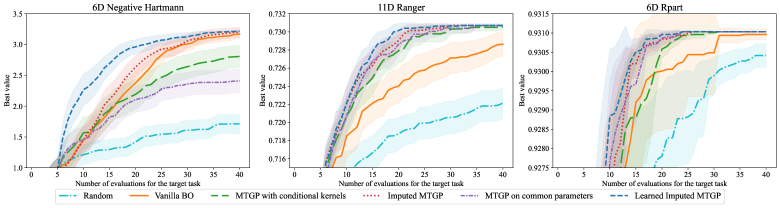
Figure 2: (Left) The Learned Imputed MTGP performs the best on the 6D Hartmann problem. (Middle/Right) The MTGP-based methods outperform Vanilla BO and Random Search on the 11D Ranger and 6D Rpart problems. Each experiment employs 30 source task trials.

Synthetic problems

Our first test problem uses the popular synthetic Hartmann6 function. We use one source task which corresponds to a 4D search space where last $2$ parameters are fixed to $0$. The target task is the original Hartmann6 problem. The results are show in the left plot of Fig. 2.

HPO-B benchmark problems

HPO-B is a large transfer learning benchmarking suite for hyperparameter optimization (Pineda et al., 2021). We construct two different test problems based on problems available in HPO-B. The first problem is Ranger, which has $11$ tunable parameters. We use search space ids $5965$ (missing parameter index 10) and $7607$ (missing parameter index $5$ and $9$) as the source tasks. The target task is search space id $5889$ with parameters [$0$, $1$, $2$, $3$, $6$, $7$]. The second problem is Rpart where we use search space ids $5636$ and $5859$ (both with all $6$ parameters) as source tasks. The target task has search space id $4796$ and only has parameters [$0$, $2$, $3$].

We use $30$ source trials from each source task, resulting in a total of $60$ source trials. The results for the Ranger and Rpart problems are shown in the middle and right plots in Fig. 2.

Code

All methods were implemented in Python using BoTorch (Balandat et al., 2020). The source code and the instructions to reproduce the benchmark results can be found in our Github repository: https://github.com/facebookresearch/heterogeneous_botl.

5.1  Ablation study

We perform an ablation study where we vary the number of source trials on the 11D Ranger problem. Fig. 3 shows the results for $10$, $30$, and $50$ source trials for each source task.

Figure 3: Ablation study for varying the number of trials for each source task on the 11D Ranger problem. We observe that the MTGP with conditional kernels performs the best when only a small number of source trials are available. As more source data is available, the Learned Imputed MTGP and MTGP on common parameters perform the best.

6  Conclusions

Our results show that BO with transfer learning can be successfully leveraged in the setting of heterogeneous search spaces where we have access to small amounts of historical data. For future work, we plan on exploring ways of leveraging additional domain-specific information. Additionally, leveraging other probabilistic models, e.g., Bayesian neural networks, may address some of the scaling limitation of our approach that come from leveraging exact MTGP models.

7  Broader Impact

After careful reflection, the authors have determined that this work presents no notable negative impacts to society or the environment.

Submission Checklist

1. For all authors…

   1. Do the main claims made in the abstract and introduction accurately reflect the paper’s contributions and scope? [Yes] The abstract and introduction focus on Bayesian optimization with transfer learning which is the setting considered in the paper.

   2. Did you describe the limitations of your work? [Yes] We point out limitations of our work in the conclusion.

   3. Did you discuss any potential negative societal impacts of your work? [Yes] We do not foresee any negative societal impact of this work since this is purely methods work. We also added the discussion in the main paper.

   4. Did you read the ethics review guidelines and ensure that your paper conforms to them? https://2022.automl.cc/ethics-accessibility/ [Yes] We confirm that we have reviewed the guidelines that our paper confirms to them

2. If you ran experiments…

   1. Did you use the same evaluation protocol for all methods being compared (e.g., same benchmarks, data (sub)sets, available resources)? [Yes] All methods use the same experimental setup. We initialize all methods with exactly the same initial seed for each replication.

   2. Did you specify all the necessary details of your evaluation (e.g., data splits, pre-processing, search spaces, hyperparameter tuning)? [Yes] We describe all necessary details in the experimental section. Furthermore, we have also provided the code and will open-source the implementation upon acceptance.

   3. Did you repeat your experiments (e.g., across multiple random seeds or splits) to account for the impact of randomness in your methods or data? [Yes] We use $100$ replications for all experiments in this paper.

   4. Did you report the uncertainty of your results (e.g., the variance across random seeds or splits)? [Yes] All our figures show the mean performance +/- 2 standard errors.

   5. Did you report the statistical significance of your results? [Yes] All experiments use $100$ replications and we plot the mean +/- 2 standard errors.

   6. Did you use tabular or surrogate benchmarks for in-depth evaluations? [Yes] We consider two benchmark problems from HPO-B dataset.

   7. Did you compare performance over time and describe how you selected the maximum duration? [N/A] We report performance as a function of the number of evaluations, which is common for Bayesian optimization.

   8. Did you include the total amount of compute and the type of resources used (e.g., type of gpus, internal cluster, or cloud provider)? [Yes] We spent a total of 6.5 CPU days of a 4-core 12 GB machine to run the experiments that were used to generate the plots in this paper. We spent a negligible amount of additional compute on exploration.

   9. Did you run ablation studies to assess the impact of different components of your approach? [Yes] We conduct an ablation study on the number of source trials to better understand how that affects performance.

3. With respect to the code used to obtain your results…

   1. Did you include the code, data, and instructions needed to reproduce the main experimental results, including all requirements (e.g., requirements.txt with explicit versions), random seeds, an instructive README with installation, and execution commands (either in the supplemental material or as a url)? [Yes] We have included a link to an anonymized repository with our code and instructions to reproduce the results, see https://anon-github.automl.cc/r/heterogeneous_botl-CD0D/

   2. Did you include a minimal example to replicate results on a small subset of the experiments or on toy data? [Yes] We included full details of how to replicate the results by running the benchmarks in the README section of the code repository.

   3. Did you ensure sufficient code quality and documentation so that someone else can execute and understand your code? [Yes] We made sure the README contains proper documentation of the code including description of formatting and testing.

   4. Did you include the raw results of running your experiments with the given code, data, and instructions? [Yes] We added all the raw results in the results directory of our code repository available at the anonymous link: https://anon-github.automl.cc/r/heterogeneous_botl-CD0D/

   5. Did you include the code, additional data, and instructions needed to generate the figures and tables in your paper based on the raw results? [Yes] We provided the code to generate the figures from raw results.

4. If you used existing assets (e.g., code, data, models)…

   1. Did you cite the creators of used assets? [Yes] We have cited HPO-B which we use for two benchmark problems. We have also cited the BoTorch paper since we leverage BoTorch both for our methods and the baselines.

   2. Did you discuss whether and how consent was obtained from people whose data you’re using/curating if the license requires it? [N/A] Both BoTorch and HPO-B are freely provided without restriction, under respective MIT licenses.

   3. Did you discuss whether the data you are using/curating contains personally identifiable information or offensive content? [N/A]

5. If you created/released new assets (e.g., code, data, models)…

   1. Did you mention the license of the new assets (e.g., as part of your code submission)? [No] We left license out of the submission to preserve anonymity during review. All code and assets will be released under MIT license upon publication.

   2. Did you include the new assets either in the supplemental material or as a url (to, e.g., GitHub or Hugging Face)? [Yes] Implementation of all models and benchmarking related code is provided via an anoymized GitHub link.

6. If you used crowdsourcing or conducted research with human subjects…

   1. Did you include the full text of instructions given to participants and screenshots, if applicable? [N/A]

   2. Did you describe any potential participant risks, with links to Institutional Review Board (irb) approvals, if applicable? [N/A]

   3. Did you include the estimated hourly wage paid to participants and the total amount spent on participant compensation? [N/A]

7. If you included theoretical results…

   1. Did you state the full set of assumptions of all theoretical results? [N/A]

   2. Did you include complete proofs of all theoretical results? [N/A]

Appendix A Example conditional kernel construction

Without loss of generality, we can assign each parameter a unique integer id. For the example from Sec. 3:

• Search space of $f_{1}$: $\mathcal{X}_{1}$ = {1: learning rate, 2: dropout rate}

• Search space of $f_{2}$ : $\mathcal{X}_{2}$ = {1: learning rate, 2: dropout rate 3: batch size}

• Search space of $f_{3}$: $\mathcal{X}_{3}$ = {1: learning rate, 2: dropout rate, 4: number of hidden layers}

This means that the universal set of parameters is $\mathcal{U}=\{1,2,3,4\}$. The conditional kernel can be constructed as follows:

1. First, we construct a set $\widetilde{\mathcal{U}}$ of size $p$ consisting of subsets of ids that are common across as many tasks as possible. For example, in the case above, $\widetilde{\mathcal{U}}=\{[1,2],[3],[4]\}$ with $p=3$. Algorithm 1 provides the pseudo-code for this procedure.

2. We define $p$ base kernels $\{k_{1},k_{2},\cdots,k_{p}\}$ for each subset in $\widetilde{\mathcal{U}}$. For example, in the case above, we define three base kernels $\{k_{1},k_{2},k_{3}\}$.

3. The conditional kernel $\mathcal{K}_{c}$ value of two inputs $x$ and $x^{\prime}$ coming from two tasks $i,i^{\prime}$ is then defined as the sum of the base kernels that correspond to the subsets containing common parameters of both task $i$ or task $i^{\prime}$:

   $$\mathcal{K}_{c}(\{x,i\},\{x^{\prime},i^{\prime}\})=\sum_{j=1}^{p}\textbf{\text{{I}}}[\widetilde{\mathcal{U}}[j]\subset\mathcal{X}_{i}\cap\subset\mathcal{X}_{i^{\prime}}]\cdot k_{j}(x[\widetilde{\mathcal{U}}[j]],x^{\prime}[\widetilde{\mathcal{U}}[j]]),$$ (1)

   where I is the indicator function that determines if the corresponding subset $\widetilde{\mathcal{U}}[j]$ is part of both tasks $\mathcal{X}_{1}$ and $\mathcal{X}_{2}$ We let $\widetilde{\mathcal{U}}[j]$ refer to the $j$th subset of $\widetilde{\mathcal{U}}$. For example, in the example above, the conditional kernel for inputs $x$ from task 1 and $x^{\prime}$ from task 2 is defined as:

   $$\mathcal{K}_{c}(\{x,i\},\{x^{\prime},i^{\prime}\})=k_{1}(x[1,2],x^{\prime}[1,2]).$$ (2)

   Similarly, if the inputs $x$ and $x^{\prime}$ are from the same task 2, the conditional kernel is:

   $$\mathcal{K}_{c}(\{x,i\},\{x^{\prime},i^{\prime}\})=k_{1}(x[1,2],x^{\prime}[1,2])+k_{2}(x[3],x^{\prime}[3])$$ (3)

Algorithm 1 Construct $\widetilde{\mathcal{U}}$: Subsets of Common Indices

1:List of parameter index lists $\mathcal{F}=[F_{1},F_{2},...,F_{t}]$ where $F_{i}$ corresponds to task $i$

2:$\text{$\widetilde{\mathcal{U}}$}\leftarrow\{\text{set}(F_{1})\}$

3:for $i\leftarrow 2$ to $n$ do

4:     $\text{idx\_set}\leftarrow\text{set}(F_{i})$

5:     $\text{new\_subsets}\leftarrow[]$

6:     for $\text{sub}\in\text{$\widetilde{\mathcal{U}}$}$ do

7:         $\text{common}\leftarrow\text{idx\_set}\cap\text{sub}$

8:         $\text{remaining}\leftarrow\text{sub}\setminus\text{common}$

9:         if $\text{common}\neq\emptyset$ then

10:              $\text{new\_subsets}.\text{append}(\text{common})$

11:              $\text{idx\_set}\leftarrow\text{idx\_set}\setminus\text{common}$

12:         end if

13:         if $\text{remaining}\neq\emptyset$ then

14:              $\text{new\_subsets}.\text{append}(\text{remaining})$

15:         end if

16:     end for

17:     if $\text{idx\_set}\neq\emptyset$ then

18:         $\text{new\_subsets}.\text{append}(\text{idx\_set})$

19:     end if

20:     $\text{$\widetilde{\mathcal{U}}$}\leftarrow\text{new\_subsets}$

21:end for

22:return $\widetilde{\mathcal{U}}$

Remark

Our approach only transfers information between the shared parameters in any two tasks. If there is no overlap, no information can be transferred as this will result in two independent sub-kernels being trained and utilized for the two tasks.

References

- Ament et al. (2023) Sebastian Ament, Samuel Daulton, David Eriksson, Maximilian Balandat, and Eytan Bakshy. Unexpected improvements to expected improvement for bayesian optimization. In Advances in Neural Information Processing Systems, volume 36, pages 20577–20612, 2023.
- Bai et al. (2023) Tianyi Bai, Yang Li, Yu Shen, Xinyi Zhang, Wentao Zhang, and Bin Cui. Transfer learning for bayesian optimization: A survey. arXiv preprint arXiv:2302.05927, 2023.
- Balandat et al. (2020) Maximilian Balandat, Brian Karrer, Daniel R. Jiang, Samuel Daulton, Benjamin Letham, Andrew Gordon Wilson, and Eytan Bakshy. BoTorch: A Framework for Efficient Monte-Carlo Bayesian Optimization. In Advances in Neural Information Processing Systems 33, 2020.
- Candelieri et al. (2018) Antonio Candelieri, Raffaele Perego, and Francesco Archetti. Bayesian optimization of pump operations in water distribution systems. Journal of Global Optimization, 71(1):213–235, 2018.
- Chen et al. (2022) Yutian Chen, Xingyou Song, Chansoo Lee, Zi Wang, Richard Zhang, David Dohan, Kazuya Kawakami, Greg Kochanski, Arnaud Doucet, Marc’aurelio Ranzato, et al. Towards learning universal hyperparameter optimizers with transformers. Advances in Neural Information Processing Systems, 35:32053–32068, 2022.
- Dai et al. (2022) Zhongxiang Dai, Yizhou Chen, Haibin Yu, Bryan Kian Hsiang Low, and Patrick Jaillet. On provably robust meta-bayesian optimization. In Uncertainty in Artificial Intelligence, pages 475–485. PMLR, 2022.
- Fan et al. (2024) Zhou Fan, Xinran Han, and Zi Wang. Transfer learning for bayesian optimization on heterogeneous search spaces. Transactions on Machine Learning Research, 2024. ISSN 2835-8856. URL https://openreview.net/forum?id=emXh4M7TyH.
- Feurer et al. (2018) Matthias Feurer, Benjamin Letham, and Eytan Bakshy. Scalable meta-learning for bayesian optimization. arXiv preprint arXiv:1802.02219, 2018.
- Frazier (2018) Peter I Frazier. A tutorial on bayesian optimization. arXiv preprint arXiv:1807.02811, 2018.
- Garnett (2023) Roman Garnett. Bayesian Optimization. Cambridge University Press, 2023. to appear.
- Hernández-Lobato et al. (2017) José Miguel Hernández-Lobato, James Requeima, Edward O. Pyzer-Knapp, and Alán Aspuru-Guzik. Parallel and distributed Thompson sampling for large-scale accelerated exploration of chemical space. In Proceedings of the 34th International Conference on Machine Learning, volume 70 of Proceedings of Machine Learning Research, pages 1470–1479. PMLR, 2017.
- Hvarfner et al. (2024) Carl Hvarfner, Erik Orm Hellsten, and Luigi Nardi. Vanilla bayesian optimization performs great in high dimension. arXiv preprint arXiv:2402.02229, 2024.
- Jones et al. (1998) Donald R. Jones, Matthias Schonlau, and William J. Welch. Efficient global optimization of expensive black-box functions. Journal of Global Optimization, 13:455–492, 1998.
- Letham et al. (2019) Benjamin Letham, Brian Karrer, Guilherme Ottoni, Eytan Bakshy, et al. Constrained Bayesian optimization with noisy experiments. Bayesian Analysis, 14(2):495–519, 2019.
- Negoescu et al. (2011) Diana M Negoescu, Peter I Frazier, and Warren B Powell. The knowledge-gradient algorithm for sequencing experiments in drug discovery. INFORMS Journal on Computing, 23(3):346–363, 2011.
- Perrone et al. (2018) Valerio Perrone, Rodolphe Jenatton, Matthias W Seeger, and Cédric Archambeau. Scalable hyperparameter transfer learning. Advances in neural information processing systems, 31, 2018.
- Pineda et al. (2021) Sebastian Pineda, Hadi Jomaa, Martin Wistuba, and Josif Grabocka. Hpo-b: A large-scale reproducible benchmark for black-box hpo based on openml. Proceedings of the Neural Information Processing Systems Track on Datasets and Benchmarks, 06 2021.
- Rasmussen et al. (2006) Carl Edward Rasmussen, Christopher KI Williams, et al. Gaussian processes for machine learning, volume 1. Springer, 2006.
- Schilling et al. (2016) Nicolas Schilling, Martin Wistuba, and Lars Schmidt-Thieme. Scalable hyperparameter optimization with products of gaussian process experts. In Machine Learning and Knowledge Discovery in Databases: European Conference, ECML PKDD 2016, Riva del Garda, Italy, September 19-23, 2016, Proceedings, Part I 16, pages 33–48. Springer, 2016.
- Shilton et al. (2017) Alistair Shilton, Sunil Gupta, Santu Rana, and Svetha Venkatesh. Regret bounds for transfer learning in bayesian optimisation. In Artificial Intelligence and Statistics, pages 307–315. PMLR, 2017.
- Snoek et al. (2012) Jasper Snoek, Hugo Larochelle, and Ryan P Adams. Practical bayesian optimization of machine learning algorithms. In Advances in neural information processing systems, pages 2951–2959, 2012.
- Song et al. (2024) Xingyou Song, Oscar Li, Chansoo Lee, Daiyi Peng, Sagi Perel, Yutian Chen, et al. Omnipred: Language models as universal regressors. arXiv preprint arXiv:2402.14547, 2024.
- Stoll et al. (2020) Danny Stoll, Jörg KH Franke, Diane Wagner, Simon Selg, and Frank Hutter. Hyperparameter transfer across developer adjustments. arXiv preprint arXiv:2010.13117, 2020.
- Swersky et al. (2013) Kevin Swersky, Jasper Snoek, and Ryan P Adams. Multi-task bayesian optimization. Advances in neural information processing systems, 26, 2013.
- Tighineanu et al. (2022) Petru Tighineanu, Kathrin Skubch, Paul Baireuther, Attila Reiss, Felix Berkenkamp, and Julia Vinogradska. Transfer learning with gaussian processes for bayesian optimization. In International Conference on Artificial Intelligence and Statistics, pages 6152–6181. PMLR, 2022.
- Turner et al. (2021) Ryan Turner, David Eriksson, Michael McCourt, Juha Kiili, Eero Laaksonen, Zhen Xu, and Isabelle Guyon. Bayesian optimization is superior to random search for machine learning hyperparameter tuning: Analysis of the black-box optimization challenge 2020. In NeurIPS 2020 Competition and Demonstration Track, 2021.
- Ueno et al. (2016) Tsuyoshi Ueno, Trevor David Rhone, Zhufeng Hou, Teruyasu Mizoguchi, and Koji Tsuda. COMBO: An efficient Bayesian optimization library for materials science. Materials discovery, 4:18–21, 2016.
- Wang et al. (2018) Zi Wang, Beomjoon Kim, and Leslie P Kaelbling. Regret bounds for meta bayesian optimization with an unknown gaussian process prior. Advances in Neural Information Processing Systems, 31, 2018.
- Wang et al. (2021) Zi Wang, George E Dahl, Kevin Swersky, Chansoo Lee, Zachary Nado, Justin Gilmer, Jasper Snoek, and Zoubin Ghahramani. Pre-trained gaussian processes for bayesian optimization. arXiv preprint arXiv:2109.08215, 2021.
- Wistuba and Grabocka (2021) Martin Wistuba and Josif Grabocka. Few-shot bayesian optimization with deep kernel surrogates. arXiv preprint arXiv:2101.07667, 2021.
- Yogatama and Mann (2014) Dani Yogatama and Gideon Mann. Efficient transfer learning method for automatic hyperparameter tuning. In Artificial intelligence and statistics, pages 1077–1085. PMLR, 2014.