SCALE at Scale: Cosmological applications of small-scale CMB lensing

Abstract

The Small-Correlated-Against-Large Estimator (SCALE) for small-scale lensing of the cosmic microwave background (CMB) provides a novel method for measuring the amplitude of CMB lensing power without the need for reconstruction of the lensing field. In our previous study, we showed that the SCALE method can outperform existing reconstruction methods to detect the presence of lensing at small scales ($\ell\gg 3000$). Here we develop a procedure to include information from SCALE in cosmological parameter inference. We construct a precise neural network emulator to quickly map cosmological parameters to desired CMB observables such as temperature and lensing power spectra and SCALE cross spectra. We also outline a method to apply SCALE to full-sky maps of the CMB temperature field, and construct a likelihood for the application of SCALE in parameter estimation. SCALE supplements conventional observables such as the CMB power spectra and baryon acoustic oscillations in constraining parameters that are sensitive to the small-scale lensing amplitude such as the neutrino mass $m_{\nu}$. We show that including estimates of the small-scale lensing amplitude from SCALE in such an analysis provides enough constraining information to measure the minimum neutrino mass at $4\sigma$ significance in the scenario of minimal mass, and higher significance for higher mass. Finally, we show that SCALE will play a powerful role in constraining models of clustering that generate scale-dependent modulation to the distribution of matter and the lensing power spectrum, as predicted by models of warm or fuzzy dark matter.

I Introduction

Forthcoming high-resolution, low-noise observations of the cosmic microwave background (CMB) will allow analysis of its gravitational lensing features to greatly exceed the precision of current measurements. Gravitational lensing is a particularly useful probe of cosmological density fluctuations, as it provides an unbiased tracer of the total mass density. CMB lensing, in particular, utilizes a very well-characterized source plane at a known redshift, and thereby is especially powerful in this regard.

In Ref. [1, hereafter C24], we developed the Small-Correlated-Against-Large Estimator (SCALE) for measuring the small-scale ($\ell\gg 3000$) lensing power in the CMB. We showed that at the sensitivity of upcoming CMB experiments, SCALE can exceed the signal-to-noise with which small-scale lensing can be measured when compared with lensing reconstruction based on the standard quadratic estimator (QE) [2, 3, 4]. SCALE is a novel method to quantify small-scale CMB lensing in high-resolution temperature maps. The basic flow of the method is to pre-process a temperature map into a map $\lambda$ of the large-scale ($\ell_{L}<3000$) gradient power which is dominated by primary CMB features, and a map $\varsigma$ of small-scale ($\ell_{S}\gg 3000$) gradient power which is dominated by lensing features. The cross-spectrum of these two maps $\Psi_{\check{L}}$ is directly related to the amplitude of the lensing power spectrum $C_{L}^{\kappa\kappa}$ of the small-scale regimes associated with $\varsigma$. We refer the reader to C24 for a complete description of the principles of SCALE as well as comparisons to measurements with quadratic estimator reconstructions [3, 5]. Throughout the paper, we will typically use $\ell$ to index multipole moments of the CMB temperature, $L$ for those of the CMB lensing field, and ${\check{L}}$ for the SCALE observables.

The value added by using SCALE compared to only utilizing conventional quadratic estimators lies in a few key areas. First, it is a simple method to quickly measure the amplitude of the small-scale CMB lensing power spectrum without the need for a full reconstruction of the lensing field. We established in C24 that SCALE outperforms quadratic estimators in terms of signal-to-noise of recovered lensing signal at small-scales in upcoming experiments. Quadratic estimators remain highly effective, tested, and well-understood tools for estimating CMB lensing on larger scales, while SCALE is presented with an opportunistic, complementary role in the realm of small-scale lensing. If one wishes to use quadratic estimators at small-scales, the reconstruction bias $N_{L}^{(1),\kappa\kappa}$ grows to similar amplitude as the lensing power spectrum $C_{L}^{\kappa\kappa}$ by $L\sim 1000$, and dominates at higher $L$ [6, 7]. The small-scale lensing regime will become ever-more important as the experimental sensitivity improves, with surveys like the upcoming Simons Observatory (SO) [8] and CMB-S4 [9, 10], as well as proposed future surveys like CMB-HD [11]. Improvements in foreground characterization and mitigation also suggest that we will be able to extract a significant amount of cosmology on these scales with appropriate statistical estimators. The maximum likelihood, maximum a posteriori, Gradient Inversion, and Bayesian techniques [12, 13, 14, 15, 16] are also currently being developed with the aim to tackle these challenges with small-scale lensing reconstruction and go beyond what the QE is capable of.

Small-scale lensing of the CMB is a particularly interesting laboratory for probing the dark matter and clustering properties of the universe (see Ref. [17] for a review of CMB lensing). The effect of massive neutrinos on the small-scale lensing power spectrum is a nearly scale-independent suppression, and an accurate measurement of the small-scale lensing amplitude will provide a valuable probe of the total neutrino mass [18, 19]. Cosmological measurement of neutrino mass is complementary to lab-based probes of neutrino mass [20] and allows for insights into physics beyond the Standard Model [21, 22]. CMB lensing probes of neutrino mass have recently taken on additional importance given hints of tighter than expected upper bounds on neutrino mass with existing cosmological data [23, 24, 25, 26, 27]. Some non-standard models of warm or fuzzy dark matter also predict a suppression of clustering on small-scales, which in turn leads to a phenomenological, scale-dependent suppression of lensing power [28, 29, 30, 31, 32, 33, 34]. These scale-dependent effects could be constrained with multiple measurements of the lensing amplitude at different scales [35, 36].

In this work, we build on the established SCALE method, and extend its application to full-sky maps. We also study its constraining power when applied to practical cosmological parameter estimation, particularly in the context of small-scale lensing. We do not include a characterization of CMB foregrounds in this work, as small-scale power added by foregrounds is not expected to correlate with the large-scale features of the primary CMB temperature field; this is still an interesting hypothesis to test, and we will leave further study of foregrounds for future work. Sampling cosmological parameters quickly requires fast predictions of theoretical spectra to compare to within the likelihood. We construct a neural network emulator and present its performance in §II. The emulator provides significant speed benefits when mapping a set of cosmological parameters to expected band-powers of angular power spectra with only a small penalty to precision ($\lesssim 0.5\%$). We present our suite of full-sky simulations for the lensed CMB in §III. We construct a likelihood for CMB temperature power spectra in a $\Lambda$CDM parameter estimation, and then extend the model to include conventional lensing reconstruction information as well as SCALE cross spectra in §IV, and present the results in §V. We additionally include an analysis with a model including a general, scale-dependent suppression of lensing at extremely small scales ($L\sim 10\,000$), and we show that SCALE can be configured to accurately detect exotic models of dark matter. Finally, we discuss the results and conclude in §VI.

II Emulation of CMB and SCALE spectra

We begin with the development of a set of emulators to quickly predict theoretical observables including the CMB lensed temperature power spectra $C_{\ell}^{TT}$, lensing power spectra $C_{L}^{\kappa\kappa}$, lensing reconstruction bias $N_{L}^{(1),\kappa\kappa}$, as well as analytic SCALE products $A_{\check{L}}$ and $\Psi_{\check{L}}$ (whose values are defined below in Eqs. (II.1) and (II.1)). The posterior sampling process typically requires upwards of $\mathcal{O}(10^{3}$ to $10^{4})$ steps per chain in order to reasonably explore a hyperspace of several cosmological parameters, and that necessitates a quick mapping from the set of parameters at each step to the relevant observables. While CMB angular power spectra can be computed quickly with existing software, repeatedly computing the expected SCALE cross-spectra with Eqs. (II.1) and (II.1) from different sets of parameters requires a significant speedup over conventional numerical integration methods. We show that neural network (NN) emulators can predict SCALE observables at the speed required for quick posterior sampling without a significant penalty in terms of accuracy. The emulators can also be trained to predict lensed CMB temperature power spectra $\tilde{C}_{\ell}^{TT}$ and lensing power spectra $C_{L}^{\kappa\kappa}$ faster than Boltzmann codes, while maintaining high accuracy.

II.1 Timing of calculations without emulators

Given a set of cosmological parameters, there are now Boltzmann codes that quickly and accurately compute primary CMB power spectra $C_{\ell}^{TT}$, lensing power spectra $C_{L}^{\phi\phi}$, and lensed CMB power spectra $\tilde{C}_{\ell}^{TT}$ (CAMB, [37]; CLASS, [38]). We opt to use CAMB in this work to keep consistency with C24, but the applications should be comparable to outputs from CLASS. Consider computing example power spectra in CAMB with lens_potential_accuracy=8 as the only non-default parameter to ensure lensing accuracy at high-$\ell$ [39]. CAMB is able to compute and return the power spectra in $\mathcal{O}(1\,{\rm s})$, with some mild dependence on the requested lmax. This is fast enough to be used in parameter estimation, but it is possible to speed up the process further by using an emulator. This is especially true if one is interested in running modified versions such as axionCAMB which take extra computational steps to include non-standard physics which could affect the small-scale lensing power spectrum and can extend the computational time by factors of anywhere from two to ten [40].

A stronger motivation for the construction of emulators for theoretical spectra comes from the application of SCALE in a cosmological likelihood. The analytic forms for SCALE products were presented in C24, and are repeated here:

$$A_{\check{L}}=\Bigg{[}2\int\frac{{\rm d}^{2}\bm{\ell}_{S}}{(2\pi)^{2}}W_{\varsigma}(\bm{\ell}_{S})W_{\varsigma}(\bm{\check{L}}-\bm{\ell}_{S})$$

$$\qquad\qquad\times\left(\bm{\ell}_{S}\cdot(\bm{\ell}_{S}-\bm{\check{L}})\right)\frac{1}{C_{\ell_{S}}^{TT,\mathrm{obs}}}\frac{1}{C_{|\bm{\check{L}}-\bm{\ell}_{S}|}^{TT,\mathrm{obs}}}$$

$$\qquad\qquad\times\int\frac{{\rm d}^{2}\bm{\ell}_{L}}{(2\pi)^{2}}W_{\lambda}(\bm{\ell}_{L})W_{\lambda}(\bm{\check{L}}-\bm{\ell}_{L})\left(\bm{\ell}_{L}\cdot(\bm{\ell}_{L}-\bm{\ell}_{S})\right)$$

$$\qquad\qquad\quad\times\left((\bm{\check{L}}-\bm{\ell}_{L})\cdot(\bm{\ell}_{S}-\bm{\ell}_{L})\right)\left(\bm{\ell}_{L}\cdot(\bm{\ell}_{L}-\bm{\check{L}})\right)$$

$$\qquad\qquad\quad\times\frac{C_{\ell_{L}}^{TT}C_{\ell_{L}}^{TT,\mathrm{fid}}}{C_{\ell_{L}}^{TT,\mathrm{obs}}}\frac{C_{|\bm{\check{L}}-\bm{\ell}_{L}|}^{TT}C_{|\bm{\check{L}}-\bm{\ell}_{L}|}^{TT,\mathrm{fid}}}{C_{|\bm{\check{L}}-\bm{\ell}_{L}|}^{TT,\mathrm{obs}}}\Bigg{]}^{-1}\,,$$ (1)

$$\left\langle\Psi_{\check{L}}\right\rangle=2A_{\check{L}}\int\frac{{\rm d}^{2}\bm{\ell}_{S}}{(2\pi)^{2}}W_{\varsigma}(\bm{\ell}_{S})W_{\varsigma}(\bm{\check{L}}-\bm{\ell}_{S})$$

$$\qquad\qquad\times\left(\bm{\ell}_{S}\cdot(\bm{\ell}_{S}-\bm{\check{L}})\right)\frac{1}{C_{\ell_{S}}^{TT,\mathrm{obs}}}\frac{1}{C_{|\bm{\check{L}}-\bm{\ell}_{S}|}^{TT,\mathrm{obs}}}$$

$$\qquad\qquad\times\int\frac{{\rm d}^{2}\bm{\ell}_{L}}{(2\pi)^{2}}W_{\lambda}(\bm{\ell}_{L})W_{\lambda}(\bm{\check{L}}-\bm{\ell}_{L})\left(\bm{\ell}_{L}\cdot(\bm{\ell}_{L}-\bm{\ell}_{S})\right)$$

$$\qquad\qquad\quad\times\left((\bm{\check{L}}-\bm{\ell}_{L})\cdot(\bm{\ell}_{S}-\bm{\ell}_{L})\right)\left(\bm{\ell}_{L}\cdot(\bm{\ell}_{L}-\bm{\check{L}})\right)$$

$$\qquad\qquad\quad\times\frac{C_{\ell_{L}}^{TT}C_{\ell_{L}}^{TT,\mathrm{fid}}}{C_{\ell_{L}}^{TT,\mathrm{obs}}}\frac{C_{|\bm{\check{L}}-\bm{\ell}_{L}|}^{TT}C_{|\bm{\check{L}}-\bm{\ell}_{L}|}^{TT,\mathrm{fid}}}{C_{|\bm{\check{L}}-\bm{\ell}_{L}|}^{TT,\mathrm{obs}}}C_{|\bm{\ell}_{S}-\bm{\ell}_{L}|}^{\phi\phi}\,,$$ (2)

where $A_{\check{L}}$ is the normalization for a cross spectrum $C_{\check{L}}^{\lambda\varsigma}$ between large-scale gradient power $\lambda$ and small-scale gradient power $\varsigma$ such that $\Psi_{\check{L}}=A_{\check{L}}C_{\check{L}}^{\lambda\varsigma}$. These equations deviate slightly from their presentation in C24; we generalize them here to include the expected SCALE response with respect to changes in cosmology (reflected in the expected primary temperature power $C_{\ell}^{TT}$) while holding our choice in filters fixed (reflected by the total observed power $C_{\ell}^{TT,\mathrm{obs}}=\tilde{C}_{\ell}^{TT,\mathrm{fid}}+N_{\ell}^{TT}$ and the expected primary temperature power at a fiducial cosmology $C_{\ell}^{TT,\mathrm{fid}}$). These integrals are constructed in a 4-dimensional Fourier space, and an implementation in which the integrals are numerically computed with the mid-point rule is provided in our publicly available package cmbpix. Consider an example computation of analytic SCALE $\Psi_{\check{L}}$ for multipoles $2<{\check{L}}<2002$ such that the width of the small-scale window for $\varsigma$ is $\ell_{S,\mathrm{max}}-\ell_{S,\mathrm{min}}=2000$, the large-scale window for $\lambda$ is $0<\ell_{L}<3000$, and each $\Psi_{\check{L}}$ is evaluated with a Riemann sum on 2-dimensional grids of $\Delta\ell_{S}=75$ and $\Delta\ell_{L}=100$. This takes $\mathcal{O}(10^{4}\,{\rm s})$ or $\mathcal{O}(10\,{\rm min})$ to compute. The numerical accuracy and computational speed of Eq. (II.1)-(II.1) is dependent on the resolution of the grid(s) on which it is evaluated. Regardless, numerically integrating the analytic SCALE products with the mid-point rule is slow enough that one would desire considerable speedups. One approach to speeding up the evaluation of Eq. (II.1)-(II.1) is to consider Monte Carlo (MC) integration. We find that a Monte Carlo integration offers a good balance of speed and accuracy and is implemented in cmbpix. One drawback of Monte Carlo integration is its non-deterministic nature, manifesting as an inherent imprecision which is dependent on the number of samples with which the integral is evaluated. We find that MC integration of Eq.(II.1)-(II.1) produces approximately $\sim 1\%$ scatter (68% region) when evaluated with $N_{\mathrm{samples}}\sim\mathcal{O}(10^{5})$ samples. This is the accuracy for the evaluation at one ${\check{L}}$ mode, and when we bin SCALE powers into bands of width $\Delta{\check{L}}=71$, we expect the scatter to be reduced by a factor of $\sqrt{\Delta{\check{L}}}\approx 8.4$. Evaluating Eq.(II.1)-(II.1) with $N_{\mathrm{samples}}=2\times 10^{5}$ within the MC integration takes $\mathcal{O}(10\,{\rm s})$. This is a significant speed-up, but a further increase in speed is desired for parameter estimation.

Emulation is further motivated if one wishes to include conventional lensing reconstruction information ($L\lesssim 1250$) from a quadratic estimator. Typically, an ‘observed’ lensing power spectrum $\hat{C}_{L}^{\kappa\kappa}$ estimated from a QE reconstruction requires the subtraction of biases $N_{L}^{(0),\kappa\kappa}$ and $N_{L}^{(1),\kappa\kappa}$ such that [3, 6, 41, 7, 42, 43]

$$C_{L}^{\kappa\kappa}\sim\hat{C}_{L}^{\kappa\kappa}-N_{L}^{(0),\kappa\kappa}-N_{L}^{(1),\kappa\kappa}.$$ (3)

The zeroth-order reconstruction bias $N_{L}^{(0),\kappa\kappa}$ includes contributions from the disconnected four-point function which is non-zero even in the absence of lensing. It is, in practice, dependent on the particular observed realization of the CMB [44], and the realization-dependent $N_{L}^{(0),\kappa\kappa,\mathrm{RD}}$ can be estimated with a combination of the observed CMB temperature power spectrum $\hat{C}_{\ell}^{TT}$ of the particular realization along with the theoretical power spectrum $C_{\ell}^{TT}$ used in the QE filters [41, 42, 45, 43, 46]. The first-order reconstruction bias $N_{L}^{(1),\kappa\kappa}$ includes non-Gaussian contributions from the connected four-point function that are not included in the quadratic estimator. For a configuration with isotropic noise, it can be analytically computed with an integral constructed in 4-dimensional Fourier space similar to Eq. (II.1)-(II.1). Two equivalent representations are derived in Refs. [6, 7]. The version from Ref. [6] for the auto-correlation of the reconstructed lensing potential field $\hat{\phi}$ with the standard temperature-temperature $(TT)$ quadratic estimator to estimate the lensing potential power $\hat{C}_{L}^{\phi\phi}$ is repeated here:

$$N_{TT,TT}^{(1),\phi\phi}(L) =\frac{A_{TT}^{2}(L)}{L^{2}}\int\frac{\mathrm{d}^{2}\bm{\ell}_{1}}{(2\pi)^{2}}\int\frac{\mathrm{d}^{2}\bm{\ell}_{1}^{\prime}}{(2\pi)^{2}}$$

$$\times F_{TT}(\bm{\ell}_{1},\bm{\ell}_{2})F_{TT}(\bm{\ell}_{1}^{\prime},\bm{\ell}_{2}^{\prime})$$

$$\times \Big{\{}C_{|\bm{\ell}_{1}-\bm{\ell}_{1}^{\prime}|}^{\phi\phi}f_{TT}(-\bm{\ell}_{1},\bm{\ell}_{1}^{\prime})f_{TT}(-\bm{\ell}_{2},\bm{\ell}_{2}^{\prime})$$

$$+C_{|\bm{\ell}_{1}-\bm{\ell}_{2}^{\prime}|}^{\phi\phi}f_{TT}(-\bm{\ell}_{1},\bm{\ell}_{2}^{\prime})f_{TT}(-\bm{\ell}_{2},\bm{\ell}_{1}^{\prime})\Big{\}}.$$ (4)

The normalization $A_{TT}$ as well as the lensing weight functions $f_{TT}$ and $F_{TT}$ are the same as those presented in Ref. [3, 6] such that $\bm{L}=\bm{\ell}_{1}+\bm{\ell}_{2}=\bm{\ell}_{1}^{\prime}+\bm{\ell}_{2}^{\prime}$ (we are considering contributions to the connected four-point function). We repeat the definitions of $A_{TT}$, $f_{TT}$, and $F_{TT}$ here:

$$A_{TT}(L)=L^{2}\Big{[}\int\frac{\mathrm{d}^{2}\bm{\ell}_{1}}{(2\pi)^{2}}f_{TT}(\bm{\ell}_{1},\bm{\ell}_{2})F_{TT}(\bm{\ell}_{1},\bm{\ell}_{2})\Big{]},$$ (5)

$$f_{TT}(\bm{\ell}_{A},\bm{\ell}_{B})=C_{\ell_{A}}^{T\nabla T}(\mathbf{L}\cdot\bm{\ell}_{A})+C_{\ell_{B}}^{T\nabla T}(\mathbf{L}\cdot\bm{\ell}_{B}),$$ (6)

$$F_{TT}(\bm{\ell}_{A},\bm{\ell}_{B})=\frac{f_{TT}(\bm{\ell}_{A},\bm{\ell}_{B})}{2C_{\ell_{A}}^{TT,\mathrm{obs}}C_{\ell_{B}}^{TT,\mathrm{obs}}},$$ (7)

where $\bm{\ell}_{A}$ and $\bm{\ell}_{B}$ can be substituted with any of $\{\bm{\ell}_{1},\bm{\ell}_{2},\bm{\ell}_{1}^{\prime},\bm{\ell}_{2}^{\prime}\}$. $f_{TT}$ is defined with respect to the expected lensing response $C_{\ell}^{T\nabla T}$ [47] which is readily computed in CAMB, and it is entirely determined by the effects of lensing on the temperature field. $F_{TT}$ represents the filter used in the quadratic estimator, and it is defined with respect to the expected lensing response $C_{\ell}^{T\nabla T}$ weighted by the total observed power $C_{\ell}^{TT,\mathrm{obs}}$. This distinction is relevant for computing the expected bias spectrum for different sets of cosmological parameters while holding the filtering fixed at a fiducial cosmology. Repeatedly computing the expected $N_{L}^{(1),\kappa\kappa}$ during parameter estimation using Eq. (4) is prohibitively slow for the same reasons as for the SCALE observables. In practice, $N_{L}^{(1),\kappa\kappa}$ is typically estimated through Monte Carlo simulations of observational noise at a fiducial cosmology, and its dependence on cosmological parameters is usually included as an approximation in the likelihood with its dependence (both directly and indirectly) on $C_{\ell}^{TT}$ and $C_{L}^{\kappa\kappa}$ [42, 43]. These approximations rely on first-order derivatives of Eq. (4) with respect to $C_{\ell}^{TT}$ and $C_{L}^{\kappa\kappa}$ which require calculations similar to Eq. (4). An emulator can quickly predict $N_{L}^{(1),\kappa\kappa}$ as computed with Eq. (4) for a wide range of cosmological parameters, which removes the need for its approximation. This approach works well for our simple models/analyses, though the Monte Carlo computation of $N_{L}^{(1),\kappa\kappa}$ and the associated approximations are well-suited for observed data which is contaminated with foregrounds, masking, etc.

II.2 Cosmological model

Consider a simple cosmological model for which conventional CMB observables can be computed with CAMB or CLASS, including the six $\Lambda$CDM parameters $\{\Omega_{c},\allowbreak\,\Omega_{b},\allowbreak\,A_{s},\allowbreak\,n_{s},\allowbreak\,h,\allowbreak\,\tau\}$ and single massive neutrino species with mass $m_{\nu}$. The chosen fiducial values are listed in Table 1. This assumed base model is a good test of the power of SCALE to constrain the small-scale lensing power, which is particularly sensitive to $m_{\nu}$ [18, 19, 22].

Table 1: The set of cosmological parameters chosen for the fiducial model.

Parameter	Symbol	Value
Reduced Hubble constant	$h$	$0.675$
Baryon density	$\Omega_{\mathrm{b}}h^{2}$	$0.022$
(Cold) Dark matter density	$\Omega_{\mathrm{c}}h^{2}$	$0.122$
Optical depth to reionization	$\tau$	$0.06$
Scalar fluctuation amplitude	$A_{\mathrm{s}}$	$2.1\times 10^{-9}$
Scalar spectral index	$n_{\mathrm{s}}$	$0.965$
Neutrino mass	$m_{\nu}$	$0.06\,{\rm eV}$
Lens suppression scale	$L_{0}$	${}^{a}\,9\,000$
Lens amplitude decay rate	$B$	${}^{a}\,0.001$
Lens suppression depth	$A_{\rm min}$	${}^{a}\,1,\,{}^{b}\,(0.25)$
Experiment noise	$w$	${}^{c}1\,\mu\mathrm{K}$-arcmin
Experiment beam	$\sigma_{b}$	${}^{c}1\,{\rm arcmin}$

^aLensing suppression parameters are held fixed at these values for base analysis, with $A_{\rm min}=1$ resulting in effectively no suppression.
^b A separate simulation with $A_{\rm min}=0.25$ was generated for analysis including lensing suppression.
^cExperimental configuration similar to a CMB-S4-like survey chosen to match the analysis of Configuration D in C24.

In addition to this base model where the lensing power spectrum is largely scaled by $m_{\nu}$, we consider a phenomenological model for scale-dependent lensing power suppression that is a feature of many dark matter models beyond the standard picture. These models are easily modeled with CAMB’s included get_partially_lensed_cls method, which applies a lensing amplitude function $A_{\rm lens}(L)$ to the non-suppressed lensing power $C_{L}^{\kappa\kappa}$ such that the suppressed lensing power spectrum $C_{L}^{\kappa\kappa,\mathrm{sup}}$ is

$$C_{L}^{\kappa\kappa,\mathrm{sup}}=A_{\rm lens}(L)C_{L}^{\kappa\kappa}.$$ (8)

We choose to model the suppression of small-scale lensing using a function similar to a logistic function, parameterized by a suppression scale $L_{0}$, lensing amplitude decay rate $B$, and suppression amplitude $A_{\rm min}$:

$$A_{\rm lens}(L)=\frac{1-A_{\rm min}}{1+\exp\left(B(L-L_{0})\right)}+A_{\rm min}.$$ (9)

This function asymptotes to unity for $L\ll L_{0}$, and to $A_{\rm min}$ for $L\gg L_{0}$, and the decay rate parameter $B$ sets the steepness of the transition. The shape of the suppression model is reminiscent of those predicted by fuzzy dark matter models as shown in e.g. Ref. [32]. Our choice in the fiducial values for the suppression model are listed in Table 1, and the corresponding $A_{\rm lens}$ is illustrated in Figure 1. This specific model exhibits a modulation in the CMB lensing power at small-scales where SCALE is particularly effective. Our emulator is capable of handling input lensing suppression parameters in each prediction, but in our base analysis we fix $A_{\rm min}=1$ to achieve effectively no suppression for all $L$. In other words, we predict power spectra with standard lensing by passing in $A_{\rm min}=1$ into our emulator. We later explicitly turn on lensing suppression for a separate analysis by including $A_{\rm min}$ as a free parameter, and generating a new simulation with an underlying value of $A_{\rm min}=0.25$, which we describe later. A visualization of the chosen suppression model is shown in Figure 1, along with a few examples where the parameters $L_{0}$, $B$, and $A_{\rm min}$ are varied individually.

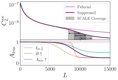
Figure 1: Top: The lensing convergence power spectrum $C_{L}^{\kappa\kappa}$ for the fiducial cosmology as computed from CAMB is compared to a model with a suppression of lensing power applied at small scales. Also shown are the three small-scale filter ranges for the applications of SCALE chosen to recover information about the lensing suppression. Bottom: The lensing amplitude $A_{\rm lens}$ applied to $C_{L}^{\kappa\kappa}$ in our suppression model is shown in dark purple (see parameters in Table 1). A version with lower $L_{0}=7\,000$ is shown in yellow. A version with higher $B=0.005$ is shown in red. A version with higher $A_{\rm min}=0.5$ is shown in green. Also shown is the fiducial model with no suppression obtained by setting $A_{\rm min}=1$.

II.3 Construction of emulators

We construct a single emulator to predict theoretical CMB (partially) lensed $TT$ power spectra $\tilde{C}_{\ell}^{TT}$, lensing convergence power spectra $C_{L}^{\kappa\kappa}$, lensing reconstruction bias $N_{L}^{(1),\kappa\kappa}$, and SCALE spectra $\Psi_{\check{L}}$ for a wide range of cosmological parameters. The emulators are created in the COMSOPOWER framework [48], which is a Python package for the construction of emulators for cosmological observables. It is based on TensorFlow [49], and it provides a structure for training and using neural network (NN) emulators.

II.3.1 Training data

The training data consist of $N_{\mathrm{train}}=8192$ sets of cosmological parameters sampled from a Latin hypercube for uniform priors in the ranges set by Table 2. This is a relatively small number of training points compared to a characteristic $N_{\mathrm{train}}=\mathcal{O}(10^{5})$ [48], but we show later that it is sufficient to train the emulators to a satisfactory degree of accuracy. The range of $\Lambda$CDM parameters is chosen to be centered on the reported Planck 2018 values with width $\pm 4.5\sigma$ [50]. We choose a training range of $[0,2]$ for the lensing suppression parameter $A_{\rm min}$, to ensure that the emulator is well-trained to recover the cosmology in the ‘vanilla’ case where $A_{\rm min}=1$ and thus where the suppression is effectively turned off as well as the case where suppression is explicitly included.

Table 2: The set of cosmological parameters and their prior ranges used to generate training data for the emulators. The $\Lambda$CDM parameters are chosen to be centered on the Planck 2018 best-fit cosmology with $\pm 4.5\sigma$ on either side [50]. Note that the emulators are trained on parameters $\Omega_{\mathrm{b}}$, $\Omega_{\mathrm{c}}$, and $\ln(10^{10}A_{s})$, but are sampled as shown as direct inputs for CAMB.

Parameter	Symbol	Prior range
Reduced Hubble constant	$h$	$[0.6493,0.6979]$
Baryon density	$\Omega_{\mathrm{b}}h^{2}$	$[0.021695,0.023045]$
(Cold) Dark matter density	$\Omega_{\mathrm{c}}h^{2}$	$[0.1146,0.1254]$
Optical depth to reionization	$\tau$	$[0.02155,0.08725]$
Scalar fluctuation amplitude	$A_{\mathrm{s}}$	$[1.965,2.235]\times 10^{-9}$
Scalar spectral index	$n_{\mathrm{s}}$	$[0.946,0.9838]$
Neutrino mass	$m_{\nu}$	$[0,0.18]\,{\rm eV}$
Lens suppression scale	$L_{0}$	$[4\,000,16\,000]$
Lens amplitude decay rate	$B$	$[10^{-4},0.05]$
Lens suppression depth	$A_{\rm min}$	[0,2]
Small-scale filter widtha	$\Delta\ell_{S}$	$[800,3200]$
Small-scale filter centera	$\overline{\ell_{S}}$	$[6200,9800]$

^aOnly affects SCALE band-powers.

For each set of parameters in our training space, we compute the following:

1. The unlensed $TT$ power spectrum $C_{\ell}^{TT}$ from CAMB for $2\leq\ell\leq 20\,000$.

2. The lensing response $C_{\ell}^{T\nabla T}$ from CAMB for $2\leq\ell\leq 8000$.

3. The suppressed lensing power spectrum $C_{L}^{\phi\phi,\mathrm{sup}}=A_{\rm lens}(L)C_{L}^{\phi\phi}$ from CAMB for $2\leq L\leq 20\,000$.

4. The partially lensed $TT$ power spectrum $\tilde{C}_{\ell}^{TT}$ from CAMB for $2\leq\ell\leq 20\,000$.

5. The quadratic estimator normalization $A_{TT}$ from pytempura [51] for $2\leq L\leq 1208$.

6. The expected lensing reconstruction bias $N_{L}^{(1),\kappa\kappa}$ from Eq. (4) with Monte Carlo integration in cmbpix for $2\leq\ell\leq 1208$.

7. The SCALE normalization $A_{\check{L}}$ from Eq. (II.1) with Monte Carlo integration in cmbpix for $2\leq{\check{L}}\leq 1989$.

8. The SCALE observables $\left\langle\Psi_{\check{L}}\right\rangle$ from Eq. (II.1) with Monte Carlo integration in cmbpix for $2\leq{\check{L}}\leq 1989$.

Table 3: Summary of binning for CMB observables.

Observable	Multipole range	Bin width	$N_{b}$
$\tilde{C}_{\ell}^{TT}$	$2\leq\ell\leq 31$	1	30
$\tilde{C}_{\ell}^{TT}$	$32\leq\ell\leq 3002$	30	99
$C_{L}^{\kappa\kappa,\mathrm{rec}}$	$2\leq L\leq 1280$	71	18
$\Psi_{\check{L}}$	$2\leq{\check{L}}\leq 1989$	71	28

We compute the (partially) lensed CMB $TT$ power spectrum out to lmax=20000 with CAMB for all $N_{\mathrm{train}}=8192$ sets of parameters in the training range, remembering to set lens_potential_accuracy=8 for high-$\ell$ accuracy [39]. The high-$\ell$ regime is required for the calculation of the SCALE quantities shown Eq. (II.1)-(II.1), which depend on the small-scale power spectra. We bin the $TT$ power spectra into band-powers following the Planck prescription [45]. The 30 largest-scale powers between $2\leq\ell\leq 31$ are kept unbinned, and the powers between $32\leq\ell\leq 3002$ are binned into 99 band-powers of width $\Delta\ell=30$. The bin weights are given by:

$$w_{\ell_{b}\ell}=\frac{\ell(\ell+1)}{\sum_{\ell\in b}\ell(\ell+1)},$$ (10)

with band-powers $\tilde{C}_{\ell_{b}}^{TT}=\sum_{\ell\in b}w_{\ell_{b}\ell}\tilde{C}_{\ell}^{TT}$ and bin centers $\ell_{b}=\sum_{\ell\in b}w_{\ell_{b}\ell}\ell$. The binning procedure is summarized in Table 3.

We also compute the CMB lensing power spectrum out to $L=20\,000$, as the small-scale $C_{L}^{\phi\phi}$ is required for the SCALE calculations. We compute the expected $N_{L}^{(1),\phi\phi}$ for each set of cosmological parameters using a Monte Carlo integration method for Eq. (4) included in cmbpix. Since the filter weight $F_{TT}$ is dependent on our choice in QE filtering, we hold it fixed in our training spectra by setting the lensing response $C_{\ell}^{T\nabla T}$ and the total observed spectrum $C_{\ell}^{TT,\mathrm{obs}}=\tilde{C}_{\ell}^{TT}+N_{\ell}^{TT}$ at the fiducial cosmology parameters described in Table 1. The dependence of $N_{L}^{(1),\phi\phi}$ on the cosmology of the training space is through the suppressed $C_{L}^{\phi\phi,\mathrm{sup}}$, along with a contribution from the lensing response $C_{\ell}^{T\nabla T}$ in $f_{TT}$ (which, as stated below Eq. 6, reflects the expected effects of lensing on the temperature field). Finally, we also compute the quadratic estimator normalization $A_{TT}$ for every set of parameters in the training space with Eq. 5. We wish to include information from conventional CMB lensing observables in our likelihood, so we save the expected ‘reconstructed’ spectrum $C_{L}^{\kappa\kappa,\mathrm{rec}}$ as band-powers with a bin width of $\Delta L=71$ between $2\leq L\leq 1208$:

$$C_{L}^{\kappa\kappa,\mathrm{rec}}=\frac{A_{TT}^{2}}{A_{TT,\mathrm{fid}}^{2}}C_{L}^{\kappa\kappa,\mathrm{sup}}+N_{L}^{(1),\kappa\kappa}.$$ (11)

The conversion between lensing potential and lensing convergence power is $C_{L}^{\kappa\kappa}=[L(L+1)]^{2}C_{L}^{\phi\phi}/4$, and $\mathcal{D}_{L}^{dd}=[L(L+1)]^{2}C_{L}^{\phi\phi}/2\pi$ is the default power spectrum returned by CAMB. The ‘reconstructed’ spectrum reflects what the lensing convergence power spectrum $C_{L}^{\kappa\kappa}$ is expected to be for a given underlying cosmology given a chosen set of fiducial parameters for filtering (after subtracting $N_{L}^{(0),\kappa\kappa}$), hence the renormalization with respect to the fiducial normalization $A_{TT,\mathrm{fid}}$ in the first term. We further discuss the physical meaning of $C_{L}^{\kappa\kappa,\mathrm{rec}}$ in §IV.

We compute expected SCALE observables for each set of parameters in our training space with Monte Carlo integration of Eq. (II.1)-(II.1) included in cmbpix. Similar to $N_{L}^{(1),\kappa\kappa}$, we hold the filter weights fixed at the fiducial cosmology: i.e., all factors of $C_{\ell}^{TT,\mathrm{fid}}$ and $C_{\ell}^{TT,\mathrm{obs}}$ in Eq. (II.1)-(II.1) are held fixed with respect to Table 1. The dependence of SCALE observables on the cosmological parameters in the training space (and by extension during parameter estimation) is through the lensing power spectrum $C_{L}^{\phi\phi}$ along with one factor each of $C_{\ell_{L}}^{TT}$ and $C_{|\bm{\check{L}}-\bm{\ell}_{L}|}^{TT}$ in the numerator of the innermost integrals of Eq. (II.1)-(II.1), which together reflect changes in the expected temperature trispectrum from lensing.

Different parts of the high-$L$ lensing power are probed by altering the filtering scheme within SCALE: we include in the emulator the dependence of SCALE observables on the small-scale filter width $\Delta\ell_{S}$ and center $\overline{\ell_{S}}$, which is equivalent to altering the limits of the outer $\ell_{S}$ integral in Eq. (II.1)-(II.1). As an example, $\ell_{S}\in[8\,000,10\,000]$ corresponds to $\Delta\ell_{S}=2\,000$ and $\overline{\ell_{S}}=9\,000$. These ‘parameters’ allow for flexibility when applying the likelihood for different SCALE data vectors constructed from the same map(s), but with different ranges of small-scale filtering. We further discuss this in §IV. We save the expected $\Psi_{\check{L}}$ for our whole training set as band-powers with a bin width of $\Delta{\check{L}}=71$ between $2\leq{\check{L}}\leq 1989$. The band-powers of all CMB observables that we include in our likelihood are summarized in Table 3.

II.3.2 Emulator performance

The emulator we construct contains 4 hidden layers, each with 512 nodes, following the default configuration for a neural network emulator in COSMOPOWER [48]. The input layer contains the 12 parameters in Table 2, and outputs are the combined 174 band-powers listed in Table 3. The relevant parameters for the emulator are converted to $\Omega_{\mathrm{b}}$, $\Omega_{\mathrm{c}}$, and $\ln(10^{10}A_{s})$ as inputs rather than their counterparts in Table 2. We include 87.5% of the full training set $N_{\mathrm{train}}=8192$ during training, with the remaining 1024 reserved for validation. The emulator takes approximately 1 min 30 s to train, and it only needs to be trained once for a given set of training spectra computed with a chosen cosmological model. The trained model can be saved and loaded for future use without retraining.

We find that the emulator performs much more quickly than the original counterparts used to compute each set of band-powers, providing predictions of their respective observables in $\mathcal{O}(10^{-3}\,{\rm s})$. Figure 2 shows that the lensed CMB $TT$ emulator is extremely precise, with a prediction error of $\lesssim 0.05\%$ per band-power. Similarly, Figure 2 shows that the emulator predicts expected reconstructed band-powers with an error of $\lesssim 0.1\%$, and the SCALE observables with a precision of $\lesssim 0.5\%$ per band-power. The values of each band-power from the emulator are predicted independently and do not correlate with one another. This applies to their scatter as well; i.e., the bin-to-bin scatter of the emulator’s predictions is uncorrelated. We attribute the lower precision of the reconstruction and SCALE band-powers to the inherent scatter of the input spectra computed with Monte Carlo integration related to the number of samples. We also find that the emulator is more accurate/precise when trained on the band-powers rather than their unbinned counterparts and then binning the full predicted spectra (a factor of $\sim 13.5\times$ more scatter for $TT$ band-powers and $\sim 1.5\times$ more scatter for the other band-powers). The scatter from predicting the full SCALE spectra multipole-by-multipole is at approximately the same level as the precision of the MC integration itself ($\sim 1\%$ before binning). Finally, the emulator exhibits an insignificant bias in its predictions, as the prediction errors effectively scatter around zero in Figure 2. A summary of the computational speedup provided by the emulator is provided in Table 4.

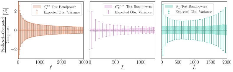
Figure 2: A validation of the emulator for our CMB observables. The % error represented here is computed as the difference between the emulator prediction and the computed output (with CAMB for $\{C_{\ell}^{TT},C_{L}^{\kappa\kappa}\}$, and Monte Carlo integration with CAMB spectra for $\{N_{L}^{(1),\kappa\kappa},\Psi_{\check{L}}\}$) divided by the computed output. We perform training using 7168 out of a set of 8192 band-powers spanning a large range of cosmological parameters outlined in Table 2. We perform validation tests using the remaining 1024 sets of band-powers unseen by the emulator during training. The filled rectangles indicate the expected 68-percentile precision centered on the median, and the bin-to-bin scatter of emulator predictions is uncorrelated. The precision of each predicted $C_{\ell}^{TT}$ band-power is generally within $0.05\%$, and these rectangles are not visible on this $y$-scale. Error bars indicate the expected observational variance of band-powers, comparable to the diagonal of the covariance matrix underlying Figure 3. There is no significant bias from the emulator’s predictions within our chosen range of cosmological parameter space, and the precision is generally better than the expected observational variance of all band-powers at our chosen level of noise.

Table 4: A comparison of computation speed for expected CMB observables. The computation time of $C_{L}^{\kappa\kappa}$ is comparable to that of $\tilde{C}_{\ell}^{TT}$. The computation times of $N_{L}^{(1),\kappa\kappa}$ and $A_{\check{L}}$ are comparable to that of $\Psi_{\check{L}}$. The emulator predicts all band-powers summarized in Table 3 at once for a given set of parameters with a significant speedup for all observables.

Computation	Time to evaluate [$\mathcal{O}({\rm s})$]
$\tilde{C}_{2<\ell<5{\rm k}}^{TT}$ (CAMB)	1
$\tilde{C}_{2<\ell<5{\rm k}}^{TT}$ (Emulator)	$10^{-3}$
$\Psi_{2<{\check{L}}<2{\rm k}}$ (cmbpix mid-point)	$10^{4}$
$\Psi_{2<{\check{L}}<2{\rm k}}$ (cmbpix Monte Carlo)	10
$\Psi_{2<{\check{L}}<2{\rm k}}$ (Emulator)	$10^{-3}$

III Simulations

We compute a suite of full-sky simulations of the lensed CMB temperature field with the lenspyx package [52, 53], which wraps around methods from DUCC (Distinctly Useful Code Collection) and allows for efficient and accurate lensing and de-lensing operations with spherical harmonics transforms [53]. A notebook with instructions to simulate the lensed CMB temperature and polarization is provided in the lenspyx repository. We choose to simulate maps with HEALPix resolution NSIDE=8192, as the lenspyx accuracy is good out to $\ell\approx 2\times\texttt{NSIDE}$. The simulations are constructed with the same fiducial cosmological parameters as shown in Table 1. We additionally apply the quadratic estimator with so-lenspipe as well as SCALE with the following procedure:

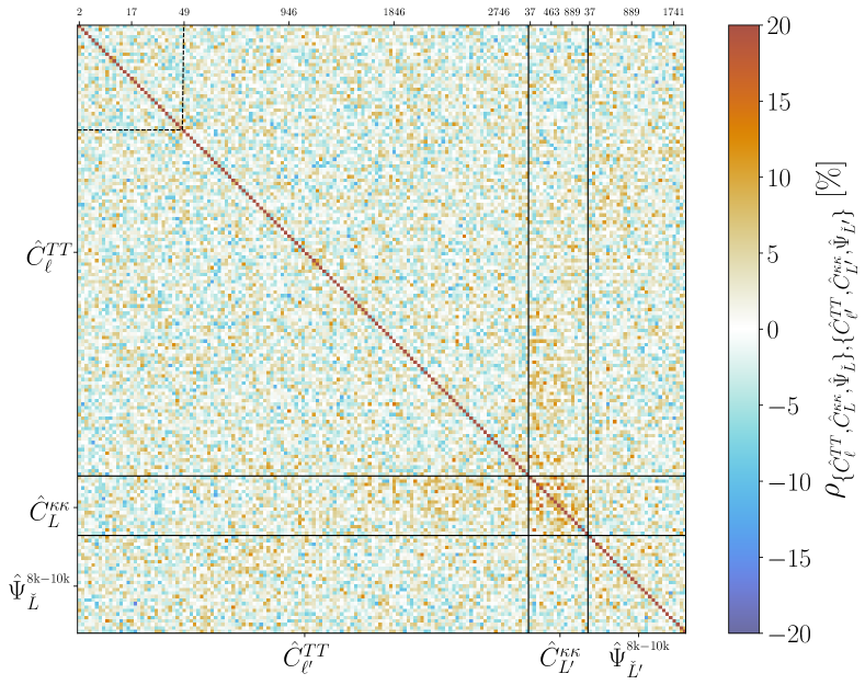
Figure 3: The correlation matrix between simulated CMB temperature, reconstructed lensing, and SCALE band-powers at the fiducial cosmology (see Table 1). The correlations are computed from 600 simulations. The band-powers are binned similarly to the Planck scheme for $\hat{C}_{\ell}^{TT}$ [45]: i.e., unbinned for $2\leq\ell\leq 31$ (sectioned with dashed lines) and with width $\Delta\ell=30$ for $32\leq\ell\leq 3002$. The reconstructed lensing band-powers $\hat{C}_{L}^{\kappa\kappa,\mathrm{rec}}$ are binned with width $\Delta L=71$ for $2\leq L\leq 1208$. SCALE band-powers $\hat{\Psi}_{\check{L}}$ are binned with width $\Delta{\check{L}}=71$ for $2\leq{\check{L}}\leq 1989$. Combinations of contributing components $\{\hat{C}_{\ell}^{TT},\hat{C}_{L}^{\kappa\kappa,\mathrm{rec}},\hat{\Psi}_{\check{L}}\}$ and their underlying covariance matrix are used in our likelihoods combining conventional CMB observables and SCALE band-powers.

1. Generate a lensed temperature field, and estimate the total ‘observed’ temperature power $\hat{C}_{\ell}^{TT}$.

   1. Compute the fiducial unlensed CMB $TT$ power spectrum $C_{\ell}^{TT}$ and lensing potential power spectrum $C_{L}^{\phi\phi}$ with CAMB out to lmax=20000 with lens_potential_accuracy=8.

   2. Generate spherical harmonic coefficients $T_{\ell m}$ and $\phi_{\ell m}$ for both an unlensed temperature $T$ using $C_{\ell}^{TT}$ and lensing potential $\phi$ field using $C_{L}^{\phi\phi}$ with synalm.

   3. Transform the lensing potential field into a spin-1 deflection field $\mathbf{d}$ with lenspyx’s almxfl method.

   4. Compute the lensed temperature field $\tilde{T}$ using the unlensed temperature $T$ and deflection $\mathbf{d}$ coefficients with alm2lenmap. This returns a lensed temperature field $\tilde{T}$ in map-space at NSIDE=8192.

   5. Generate spherical harmonic coefficients $N_{\ell m}$ for a Gaussian noise temperature field $N$ with synalm (noise parameters also in Table 1), convert to map-space with alm2map, and add to the lensed temperature field $T^{\mathrm{obs}}=\tilde{T}+N$.

   6. Convert the observed temperature field $T^{\mathrm{obs}}$ to spherical harmonic coefficients $T_{\ell m}^{\mathrm{obs}}$ using map2alm, and estimate the total ‘observed’ $TT$ power spectrum $\hat{C}_{\ell}^{TT}$ with alm2cl, which is saved.

2. Apply the quadratic estimator, and estimate the reconstructed lensing power spectrum $\hat{C}_{L}^{\kappa\kappa,\mathrm{rec}}=\hat{C}_{L}^{\kappa\kappa}+N_{L}^{(0),\kappa\kappa,\mathrm{RD}}$.

   1. Apply an isotropic filter to $T_{\ell m}^{\mathrm{obs}}$ with the expected lensing response $C_{\ell}^{T\nabla T}$ such that $2\leq\ell\leq 3000$ to get $T_{\ell m}^{\mathrm{filt}}$.

   2. Reconstruct the lensing potential field $\phi_{\ell m}^{\mathrm{rec}}$ from $T_{\ell m}^{\mathrm{filt}}$ with so-lenspipe, and estimate the reconstructed lensing power spectrum $\hat{C}_{L}^{\kappa\kappa}$ with alm2cl.

   3. Compute the realization dependent $N_{L}^{(0),\kappa\kappa,\mathrm{RD}}$ using the observed temperature power spectra $\hat{C}_{\ell}^{TT}$ with so-lenspipe.

   4. Save the total reconstructed lensing power spectrum $\hat{C}_{L}^{\kappa\kappa,\mathrm{rec}}=\hat{C}_{L}^{\kappa\kappa}-N_{L}^{(0),\kappa\kappa,\mathrm{RD}}$.

3. Apply SCALE, and estimate the cross-spectrum between the large-scale temperature gradient, and the small-scale temperature gradient $\Psi_{\check{L}}=A_{\check{L}}C_{\check{L}}^{\lambda\varsigma}$.

   1. Apply a low-pass filter such that $0<\ell_{L}<3000$ along with a Wiener filter to the observed temperature field $T_{\mathrm{obs}}$ ($W_{\lambda}(\ell)$, shown below as Eq. (12)) with almxfl. The product is a set of spherical harmonic coefficients, that when converted to map space with a spin-1 inverse transform alm2map_spin, produces the two large-scale gradient components $[\nabla_{\theta}T_{L},\nabla_{\phi}T_{L}/\sin\theta]$ that make up the $\lambda=(\nabla_{\theta}T_{L})^{2}+(\nabla_{\phi}T_{L}/\sin\theta)^{2}$ map of large-scale temperature gradient power required for one half of SCALE. Note that the filter is constructed with the theoretical spectra from Step A1 using CAMB, and follow the fiducial cosmology in Table 1.

      $$W_{\lambda}(\ell)=\begin{cases}\sqrt{\ell(\ell+1)}\frac{C_{\ell}^{TT}}{\tilde{C}_{\ell}^{TT}+N_{\ell}^{TT}}&,~{}\ell<3000\\ 0&,~{}\ell\geq 3000\end{cases}\,.$$ (12)

   2. Convert the $\lambda$ map into spherical harmonic space with map2alm.

   3. Apply a high-pass filter such that $\ell_{S,{\rm min}}<\ell_{S}<\ell_{S,{\rm max}}$ along with an inverse variance filter to the observed temperature field $T_{\mathrm{obs}}$ (shown below as Eq. (13)) with almxfl. The product is a set of spherical harmonic coefficients, that when converted to map space with a spin-1 inverse transform alm2map_spin, produces the two small-scale gradient components $[\nabla_{\theta}T_{S},\nabla_{\phi}T_{S}/\sin\theta]$ that make up the $\varsigma=(\nabla_{\theta}T_{S})^{2}+(\nabla_{\phi}T_{S}/\sin\theta)^{2}$ map of small-scale temperature gradient power required for the other half of SCALE. Note that the filter is constructed with the theoretical spectra from Step A1 using CAMB, and follow the fiducial cosmology in Table 1.

      $$W_{\varsigma}(\ell)=\begin{cases}\sqrt{\ell(\ell+1)}\frac{1}{\tilde{C}_{\ell}^{TT}+N_{\ell}^{TT}}&,~{}\ell_{1,{\rm min}}<\ell_{1}<\ell_{1,{\rm max}}\\ 0&,~{}\mathrm{else}\end{cases}\,.$$ (13)

   4. Convert the $\varsigma$ map into spherical harmonic space with map2alm.

   5. Estimate the cross spectrum $\hat{C}_{\check{L}}^{\lambda\varsigma}$ between $\lambda$ and $\varsigma$ with alm2cl, and multiply by $A_{\check{L}}$ to get $\hat{\Psi}_{\check{L}}$ then save.

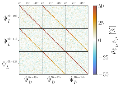
Figure 4: The correlation matrix between SCALE band-powers at the fiducial cosmology (see Table 1). The correlations between three applications of SCALE are depicted here, with shared large-scale filters $2\leq\ell_{L}\leq 3000$ and different small-scale filters indicated by superscripts. The correlations are computed from 600 simulations. The strongest off-diagonal entries indicate that SCALE band-powers at the same ${\check{L}}$ are approximately 20-50% correlated between applications of small-scale filters which share half of their multipole coverage. Correlations between SCALE with the other $\ell_{S}$ filters $\{\hat{\Psi}_{\check{L}}^{9\mathrm{k}\mathchar 45\relax 11\mathrm{k}},\hat{\Psi}_{\check{L}}^{10\mathrm{k}\mathchar 45\relax 12\mathrm{k}}\}$ and the other CMB observables $\{\hat{C}_{\ell}^{TT},\hat{C}_{L}^{\kappa\kappa,\mathrm{rec}}\}$ are similar to those of $\hat{\Psi}_{\check{L}}^{8\mathrm{k}\mathchar 45\relax 10\mathrm{k}}$ in Figure 3.

We show in §IV that, in principle, Part C may be repeated on the same realization with various choices in the small-scale $\ell_{S,{\rm min}}<\ell_{S}<\ell_{S,{\rm max}}$ filter limits, and included in the same likelihood. We include three applications of SCALE for each realization: $8\,000<\ell_{S}<10\,000$, $9\,000<\ell_{S}<11\,000$, $10\,000<\ell_{S}<12\,000$, and apply their appropriate normalization $A_{\check{L}}$ from Eq. (II.1). We repeat the above procedure for 600 simulations, and we save our CMB observables as band-powers of $\{\hat{C}_{\ell}^{TT},\allowbreak\hat{C}_{L}^{\kappa\kappa,\mathrm{rec}},\hat{\Psi}_{\check{L}}^{8\mathrm{k}\mathchar 45\relax 10\mathrm{k}},\hat{\Psi}_{\check{L}}^{9\mathrm{k}\mathchar 45\relax 11\mathrm{k}},\hat{\Psi}_{\check{L}}^{10\mathrm{k}\mathchar 45\relax 12\mathrm{k}}\}$ following Table 3. The correlation matrix between $\{\hat{C}_{\ell}^{TT},\allowbreak\hat{C}_{L}^{\kappa\kappa,\mathrm{rec}},\hat{\Psi}_{\check{L}}^{8\mathrm{k}\mathchar 45\relax 10\mathrm{k}}\}$ is shown in Figure 3. The correlation between SCALE observables and the other CMB observables is generally smaller than about $5\%$. This suggests that SCALE includes unique cosmological information from the small-scale CMB lensing. Note that this information is intentionally excluded from our quadratic estimator configuration because we showed in C24 that SCALE will outperform the QE at small-scales, and we wish to study how well SCALE can fulfill its role there.

We find that the SCALE observables exhibit very low levels of covariance between band-powers, as we found with the flat-sky simulations in C24. However, band-powers at the same ${\check{L}}$ across small-scale filters with overlapping $\ell_{S}$ ranges (e.g., $\hat{\Psi}_{\check{L}}^{8\mathrm{k}\mathchar 45\relax 10\mathrm{k}}$ and $\hat{\Psi}_{\check{L}}^{9\mathrm{k}\mathchar 45\relax 11\mathrm{k}}$ for at the same ${\check{L}}$) are highly correlated, with off-diagonal entries of approximately 20-50%. This is shown in Figure 4, and it implies that applying SCALE with different small-scale filter ranges indeed characterizes different parts of the lensing power spectrum.

We additionally produce one more set of CMB observables with a separate realization following the above steps. This extra realization serves as the data vector that will be used in subsequent sections for cosmological inference, and is not included in the construction of the covariance/correlation matrices. A comparison of this realization’s observable band-powers with the theoretical values at the fiducial cosmology is shown in Figure 5. We produce one final set of CMB observables with a realization that includes a lensing suppression $C_{L}^{\kappa\kappa,\mathrm{sup}}$ in Step A2 with $A_{\rm min}=0.25$, and all other parameters following Table 1. This realization is used later to test SCALE’s ability to constrain more exotic small-scale clustering phenomena.

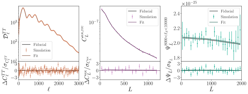
Figure 5: A comparison between predicted CMB observable band-powers from the emulator at the fiducial cosmology with a set of band-powers computed from simulation. The simulated band-powers are overlaid with error-bars corresponding to the diagonal of Figure 3. Predicted band-powers at the best fit cosmology from combining all three observables in §V are also shown. The residuals with respect to the fiducial band-powers are shown in the bottom panels. The ‘observed’ band-powers from simulation match well with both the fiducial and best fit values.

IV Constructing a Likelihood with SCALE

Consider a model defined by $\Lambda$CDM cosmology with the addition of one neutrino mass eigenstate parameterized with $m_{\nu}$. The general suppression of small-scale lensing due to the massive neutrino offers a simple test of SCALE’s constraining power. Our initial vector of parameters is $\vec{\theta}=\{m_{\nu},\allowbreak\,\Omega_{c},\allowbreak\,\Omega_{b},\allowbreak\,\ln(10^{10}A_{s}),\allowbreak\,n_{s},\allowbreak\,h,\allowbreak\,\tau\}$. The theoretical model that our emulator is trained on generally includes the lensing suppression at small scales, but for our initial analysis, we fix the relevant parameters $\vec{\theta}_{\mathrm{sup}}=\{L_{0},B,A_{\mathrm{min}}\}$ to their fiducial values in Table 1. In particular, setting $A_{\mathrm{min}}=1$ effectively turns off the lensing suppression. There is an implicitly constrained parameter $\Omega_{\Lambda}$ such that $\Omega_{c}+\allowbreak\Omega_{b}+\allowbreak\Omega_{\nu}+\Omega_{\Lambda}=1$. Our initial data vector $\vec{d}=\{\hat{C}_{\ell}^{TT},\hat{C}_{L}^{\kappa\kappa,\mathrm{rec}},\allowbreak\,\hat{\Psi}_{\check{L}}^{8\mathrm{k}\mathchar 45\relax 10\mathrm{k}}\}$ is composed of $TT$, QE reconstruction, and SCALE band-powers. We have constructed an emulator in §II to predict the theoretical expected band-powers given a set of cosmological parameters: $\vec{t}(\vec{\theta})$. Finally, we have empirical estimates of the covariance between all band-powers of the data vector from our set of simulations in §III: $\mathbf{C}$. This allows us to construct a multivariate normal log-likelihood for the data vector $\vec{d}$ given a set of parameters $\vec{\theta}$:

$$\log p(\vec{d}|\vec{\theta}) \sim\log\mathcal{N}(\vec{d}|\vec{t}(\vec{\theta}),\hat{\mathbf{C}}^{-1})$$

$$\sim-\frac{1}{2}(\vec{d}-\vec{t}(\vec{\theta}))^{T}\hat{\mathbf{C}}^{-1}(\vec{d}-\vec{t}(\vec{\theta}))\,.$$ (14)

Note that the covariance $\mathbf{C}$ is estimated from $N_{\mathrm{sims}}=600$ realizations, and the unbiased estimator for the inverse covariance must include the Hartlap factor [54]:

$$\hat{\mathbf{C}}^{-1}=\frac{N_{\mathrm{sims}}-P-2}{N_{\mathrm{sims}}-1}\mathbf{C}^{-1}\,,$$ (15)

where $P$ is the number of band-powers included in the data vector. There are $P_{TT}=129$ $TT$ band-powers, $P_{\mathrm{QE}}=17$ QE band-powers, and $P_{\mathrm{SCALE}}=28$ band-powers for each application (with different small-scale $\ell_{S}$ filters) of SCALE. It is recommended that there is a minimum of realizations $N_{\mathrm{sims}}\gtrsim 2P$ to estimate the inverse covariance, which we have satisfied [54].

The likelihood we apply compares the estimated QE reconstructed spectrum (when included) as

$$C_{L}^{\kappa\kappa,\mathrm{rec}}=\frac{A_{TT}^{2}}{A_{TT,\mathrm{fid}}^{2}} C_{L}^{\kappa\kappa}+N_{L}^{(1),\kappa\kappa}$$

$$\sim\hat{C}_{L}^{\kappa\kappa}-N_{L}^{(0),\kappa\kappa,\mathrm{RD}}=\hat{C}_{L}^{\kappa\kappa,\mathrm{rec}}\,,$$ (16)

with $C_{L}^{\kappa\kappa,\mathrm{rec}}$ predicted by our emulator as a function of a given set of parameters $\vec{\theta}$, and $\hat{C}_{L}^{\kappa\kappa,\mathrm{rec}}$ estimated directly from each realization. In practice (e.g., with the ACT and Planck lensing analyses [42, 43]), the QE-relevant quantities are directly compared to the expected CMB lensing power spectrum $C_{L}^{\kappa\kappa}$ as expressed in Eq. (3). Our construction includes the dependence of $N_{L}^{(1),\kappa\kappa}$ on parameters directly on the theory side of the likelihood because the emulator allows us to quickly determine the expected reconstruction bias for each given set of parameters. This is in contrast to a more practical likelihood, which includes $N_{L}^{(1),\kappa\kappa}$ and its dependence on cosmological parameters as first-order corrections (with respect to the dependence of $N_{L}^{(1),\kappa\kappa}$ on $C_{\ell}^{TT}$ and $C_{L}^{\kappa\kappa}$) to the observed quantities due to challenges with repeatedly computing $N_{L}^{(1),\kappa\kappa}$ [42, 45, 46]. Our construction is equivalent to the practical likelihood in the limit of well-controlled, isotropic noise, and the usual treatment of $N_{L}^{(1),\kappa\kappa}$ is preferred for real data analysis (notably with the presence of foregrounds).

We set broad and uniform priors $p_{\mathrm{Uni}}(\vec{\theta})$ for every parameter in $\vec{\theta}$ following Table 2 except for $\tau$, for which we impose a Gaussian prior about the fiducial value (Table 1):

$$p(\tau)\sim\mathcal{N}(0.06,\sigma_{\tau})\,,$$ (17)

where we choose either $\sigma_{\tau}=0.007$ set by the value reported by Planck 2018 [50], or $\sigma_{\tau}=0.002$ set by the cosmic variance limit [55]. We also include an additional likelihood which includes forecasted constraints from Baryon Acoustic Oscillation (BAO) information from the 5-year survey of the Dark Energy Spectroscopic Instrument (DESI, [56]), which mainly constrains the matter density $\Omega_{m}$. We follow the steps in Appendix V of Ref. [57] to construct a Fisher matrix $\mathbf{F}$ for BAO observables and the covariances between our other parameters, including $m_{\nu}$, $\Omega_{c}$, $\Omega_{b}$, and $h$. The BAO log-likelihood is constructed as follows:

$$\log p_{\mathrm{BAO}}(\vec{\theta}|\mathbf{F})\sim-\frac{1}{2}(\vec{\theta}-\vec{\theta}_{\mathrm{fid}})^{T}\mathbf{F}(\vec{\theta}-\vec{\theta}_{\mathrm{fid}})\,,$$ (18)

where $\vec{\theta}_{\mathrm{fid}}$ is the vector of fiducial parameters from Table 1. Our final posterior is then expressed by the following:

$$p(\vec{\theta}|\vec{d})\sim\mathcal{N}(\vec{d}|\vec{t}(\vec{\theta}),\hat{\mathbf{C}}^{-1})\mathcal{N}(\tau|0.06,\sigma_{\tau})p_{\mathrm{BAO}}(\vec{\theta}|\mathbf{F})p_{\mathrm{Uni}}(\vec{\theta})\,.$$ (19)

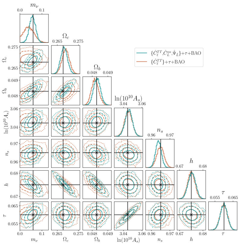
Figure 6: The sampled posterior distribution of the probabilistic model described in Eq. (19) using the $TT$ band powers along with a cosmic variance $\tau$ prior $\sigma_{\tau}=0.002$, and BAO likelihood is shown in brown. The resulting sampled posterior distribution with the addition of lensing information from both lensing reconstruction and SCALE is shown in green. The contours indicate the 68% (solid), 95% (dashed) and 99.7% (dotted) regions of a kernel density estimate for each 2-dimensional marginalized posterior. The fiducial values are indicated with black lines and $\times$ symbols. The addition of CMB lensing observables makes the difference in a detection of the minimum neutrino mass $m_{\nu}$ (see Figure 7). We also see that the covariances between matter clustering related parameters such as $m_{\nu}$, $\Omega_{c}$ and $\Omega_{b}$ tighten up with the addition of lensing observables.

Table 5: Summary of cosmological parameter constraints from combinations of the observed TT, QE reconstructed, and SCALE band-powers, along with $\tau$ and BAO priors. Fiducial values from Table 1 are also shown for comparison. The cosmic variance $\tau$ prior $\sigma_{\tau}^{\mathrm{CV}}=0.002$ [55] is used here. Reported values are the median and 68% credibility interval of each marginalized posterior. The median values of the posterior slightly shift around the fiducial values depending on the realization, but in general the shifts are comfortably within the 68% credibility intervals. The widths of the 68% regions do not change appreciably between realizations.

Parameter	Fiducial	$\hat{C}_{\ell}^{TT}$	$\hat{C}_{\ell}^{TT},\hat{C}_{L}^{\kappa\kappa,\mathrm{rec}}$	$\hat{C}_{\ell}^{TT},\hat{\Psi}_{\check{L}}^{8\mathrm{k}\mathchar 45\relax 10\mathrm{k}}$	$\hat{C}_{\ell}^{TT},\hat{C}_{L}^{\kappa\kappa,\mathrm{rec}},\hat{\Psi}_{\check{L}}^{8\mathrm{k}\mathchar 45\relax 10\mathrm{k}}$
$m_{\nu}$ [eV]	0.06	$0.041_{-0.023}^{+0.024}$	$0.045_{-0.015}^{+0.015}$	$0.066_{-0.015}^{+0.015}$	$0.057_{-0.014}^{+0.014}$
$\Omega_{c}$	$0.2678$	$0.2690_{-0.0017}^{+0.0017}$	$0.2688_{-0.0016}^{+0.0016}$	$0.2681_{-0.0015}^{+0.0016}$	$0.2682_{-0.0016}^{+0.0016}$
$\Omega_{b}$	$0.04829$	$0.04818_{-0.0002}^{+0.0002}$	$0.04820_{-0.0002}^{+0.0002}$	$0.04829_{-0.0003}^{+0.0003}$	$0.04831_{-0.0002}^{+0.0002}$
$\ln(10^{10}A_{s})$	$3.045$	$3.045_{-0.004}^{+0.004}$	$3.045_{-0.004}^{+0.004}$	$3.044_{-0.004}^{+0.004}$	$3.046_{-0.004}^{+0.004}$
$n_{s}$	$0.965$	$0.965_{-0.002}^{+0.002}$	$0.965_{-0.002}^{+0.002}$	$0.966_{-0.002}^{+0.002}$	$0.964_{-0.002}^{+0.002}$
$h$	$0.675$	$0.675_{-0.002}^{+0.002}$	$0.675_{-0.002}^{+0.002}$	$0.675_{-0.002}^{+0.002}$	$0.675_{-0.002}^{+0.002}$
$\tau$	$0.06$	$0.060_{-0.002}^{+0.002}$	$0.060_{-0.002}^{+0.002}$	$0.060_{-0.002}^{+0.002}$	$0.060_{-0.002}^{+0.002}$

In principle, the data vector $\vec{d}$, covariance matrix $\mathbf{C}$, and theory vector constructed from emulators $\vec{t}(\vec{\theta})$ can contain any combination of $TT$, QE, and SCALE band-powers as long as all three are constructed consistently. We present in §V results from several combinations of observable band-powers. We only consider one application of SCALE with $\ell_{S,{\rm min}}=8\,000$ and $\ell_{S,{\rm max}}=10\,000$ for our initial analysis. The model including a massive neutrino simply shifts the amplitude of the lensing potential power in the small-scale regime that we consider, so a single SCALE estimator is sufficient.

Including multiple applications of SCALE with different $\ell_{S,{\rm min}}$ and $\ell_{S,{\rm max}}$ in a single fit should allow for constraints on models which change the shape of the lensing power spectrum $C_{L}^{\kappa\kappa}$. To test this, we perform a separate analysis including the other two applications of SCALE in our likelihood with a full covariance combining Figure 3 and Figure 4. A separate data vector from the realization in §III with lensing suppression following Table 1 with $A_{\mathrm{min}}=0.25$ is used, and we allow the relevant parameters $\vec{\theta}_{\mathrm{sup}}$ to be free and sampled. We sample the logarithm of the decay rate parameter $\ln(B)$ to allow a larger dynamic range.

We construct and sample our probabilistic model with the Python implementation of Markov Chain Monte Carlo (MCMC) techniques in emcee [58]. We choose to use emcee rather than more commonly-used software designed specifically for cosmology such as CosmoMC [59] or cobaya [60, 61] because it offers a simple way to construct log-probabilities with the added flexibility of allowing for the use of black-box functions in the model. The latter point is essential in order to use the emulator constructed in §II at each step of the chain. We use 14 walkers, or chains if holding $\vec{\theta}_{\mathrm{sup}}$ fixed, and 20 walkers if $\vec{\theta}_{\mathrm{sup}}$ are free and sampled. Each chain is run for 50 000 steps each. The first 1 000 steps are discarded as burn-in steps that have yet to converge, and we further thin the chains by a factor of 50 to reduce the auto-correlation between samples. We find that the chains converge (satisfying the Gelman-Rubin ratio requirement $R<1.1$) after approximately 1 000 steps post-burn-in and before thinning. The results of each model are presented in §V.

V Results

The results for our base model fits using the realization of observables presented in Figure 5 are summarized in Table 5 and Figure 6-7. The band-powers as predicted by our emulator for the best-fit including all three observables is also included in Figure 5. We find that the size of the 68% region for the best fit results do not change appreciably if we choose a different realization for the data vector. The center of the best fit can vary slightly between realizations, but the change is generally well within the 68% range. The base model allows the $TT$ band-powers, combined with the BAO likelihood and $\tau$ prior, to constrain most of the parameters $\vec{\theta}$ to high precision in the presence of noise levels similar to that expected from CMB-S4 [9, 10]. The exception is $m_{\nu}$, for which the $TT$-only model with either a Planck 2018 prior or a cosmic variance prior on $\tau$ is not able to detect (see Figure 7). We also see in Figure 6 and Figure 7 that the marginalized posterior for $m_{\nu}$ using only the $TT$ band-powers as observables causes the distribution to hit the edge of the prior at $0\,{\rm eV}$.

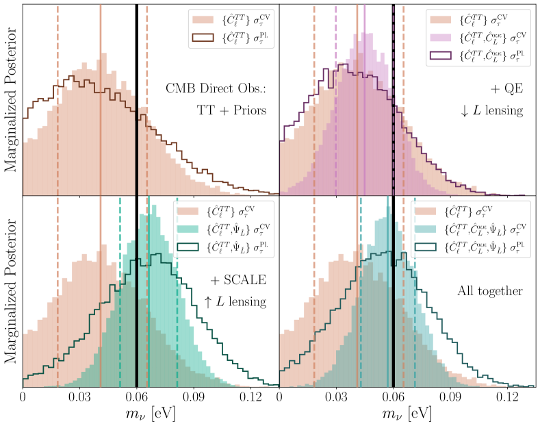
Figure 7: The marginalized posteriors (with the cosmic variance $\tau$ prior $\sigma_{\tau}=0.002$) for $m_{\nu}$ with various combinations of CMB observables. The median of each result is indicated with solid vertical lines of their respective colours, and coloured, dashed lines indicate their 68% credible intervals. A vertical black line indicates the fiducial value at $m_{\nu}=0.06\,{\rm eV}$. The marginalized posteriors using the Planck 2018 $\tau$ prior $\sigma_{\tau}=0.007$ are shown in each respective panel with step histograms (medians and 68% intervals not shown). With the condition of a precise $\tau$ estimate, the addition of lensing band-powers in general tightens the distribution of the marginalized posterior enough for a $4\sigma$ detection of minimum mass. The physical effect of neutrino mass is a mostly scale-independent change to the lensing amplitude, so this is true regardless of whether this lensing information comes from the QE reconstruction (top right), SCALE (bottom left), or both (bottom right).

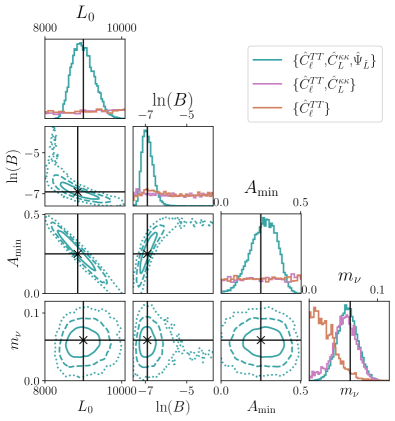
Figure 8: The partially marginalized, sampled posterior for a simulation/model with suppressed lensing at small scales as depicted in Figure 1. All six $\Lambda$CDM parameters were also sampled with results similar to Figure 6, so they are not shown here. Including just a lensing reconstruction at large-scales provides sufficient information to constrain $m_{\nu}$. Only the full set of 3 SCALE band-powers (small-scales filtered for $\ell_{S}\in\{8\mathrm{k}\mathchar 45\relax 10\mathrm{k},9\mathrm{k}\mathchar 45\relax 11\mathrm{k},10\mathrm{k}\mathchar 45\relax 12\mathrm{k}\}$) provides constraining information about this particular 3-parameter suppression model.

Table 6: Summary of cosmological parameter constraints on a model with small-scale lensing suppression from the observed TT, QE reconstructed, and SCALE band-powers, along with $\tau$ and BAO priors. Fiducial values from Table 1 are also included. The cosmic variance $\tau$ prior $\sigma_{\tau}^{\mathrm{CV}}=0.002$ [55] is used here. Reported values are the median and 68% credibility interval of each marginalized posterior. The median values of the fit slightly shift around the fiducial values depending on the realization, but in general the shifts are comfortably within the 68% credibility intervals. The widths of the 68% regions do not change appreciably between realizations.

Parameter	Fiducial	$\hat{C}_{\ell}^{TT},\hat{C}_{L}^{\kappa\kappa,\mathrm{rec}},\hat{\Psi}_{\check{L}}^{8\mathrm{k}\mathchar 45\relax 10\mathrm{k}},\hat{\Psi}_{\check{L}}^{9\mathrm{k}\mathchar 45\relax 11\mathrm{k}},\hat{\Psi}_{\check{L}}^{10\mathrm{k}\mathchar 45\relax 12\mathrm{k}}$
$L_{0}$	9000	$8977_{-264}^{+309}$
$10^{3}B$	1.00	$1.00_{-0.21}^{+0.34}$
$A_{\mathrm{min}}$	0.25	$0.27_{-0.09}^{+0.08}$
$m_{\nu}$ [eV]	0.06	$0.056_{-0.015}^{+0.015}$
$\Omega_{c}$	$0.2678$	$0.2678_{-0.0016}^{+0.0016}$
$\Omega_{b}$	$0.04829$	$0.04835_{-0.0002}^{+0.0002}$
$\ln(10^{10}A_{s})$	$3.045$	$3.042_{-0.004}^{+0.004}$
$n_{s}$	$0.965$	$0.966_{-0.002}^{+0.002}$
$h$	$0.675$	$0.675_{-0.002}^{+0.002}$
$\tau$	$0.06$	$0.060_{-0.002}^{+0.002}$

The addition of SCALE into the data vector affects the parameters most sensitive to lensing (see Figure 6): $m_{\nu}$, $\Omega_{c}$, and $\Omega_{b}$. We see that the addition of SCALE alters the degeneracies between these parameters to become more constraining. Perhaps the most salient effect of including SCALE is the added ability to provide evidence for non-zero $m_{\nu}$ at $2.4\sigma$ with the Planck $\tau$ prior. The effect is more prominent if we swap the $\tau$ prior to the cosmic variance limit $\sigma_{\tau}=0.002$ (see Table 5), which is forecasted to be achievable with upcoming data from the LiteBIRD satellite mission [55] or the CLASS ground-based survey [62]. In this case the detection jumps to a signal-to-noise of $4\sigma$ with the inclusion of SCALE. We have thus demonstrated that the addition of small-scale lensing information with SCALE provides extra constraining power for parameters which alter the lensing amplitude at $\ell\gg 3000$.

Finally, we present the results of our lensing suppression analysis in Figure 8 and Table 6. We find that the three sets of SCALE band-powers with different small-scale filtering regimes provides sufficient information to well-constrain the three parameters of our general lensing suppression model. This is the case even though the small-scale regimes we consider are overlapping, and technically share similar information about the small-scale lensing power spectrum. We find that the three lensing suppression parameters $\vec{\theta}_{\mathrm{sup}}$ are not well constrained if we perform the same analysis with a data vector consisting of only two of the applications of SCALE: for example with $\vec{d}=\{\hat{C}_{\ell}^{TT},\hat{C}_{L}^{\kappa\kappa,\mathrm{rec}},\hat{\Psi}_{\check{L}}^{8\mathrm{k}\mathchar 45\relax 10\mathrm{k}},\hat{\Psi}_{\check{L}}^{10\mathrm{k}\mathchar 45\relax 12\mathrm{k}}\}$. This is expected due to our three-parameter model requiring at least three measured amplitudes of the small-scale lensing power spectrum to constrain. In a similar vein, the same analysis with only conventional CMB observables $\{\hat{C}_{\ell}^{TT},\hat{C}_{L}^{\kappa\kappa,\mathrm{rec}}\}$ leaves the lensing suppression parameters $\vec{\theta}_{\mathrm{sup}}$ completely unconstrained, as they do not provide any information about the small-scale lensing power spectrum by construction.Therefore, with the choice of simulated data employed here, the SCALE observables provide unique constraining power in the small-scale lensing regime.

VI Discussion and Conclusions

In this paper we explored applications of the SCALE estimator to cosmological parameter estimation, and how much information SCALE provides on top of more conventional methods for CMB lensing measurement. We originally developed SCALE in C24 as a novel estimator for the amplitude of CMB lensing power at small-scales $\ell\gg 3000$. The small-scale lensing regime has yet been untouched by conventional lensing reconstruction methods alone due to limits in instrument sensitivity and concerns with foreground contamination. We showed in C24 that SCALE will outperform conventional quadratic estimators in this regime for upcoming/future experiments in terms of the signal-to-noise of a lensing amplitude measurement. While we expect that small-scale foregrounds do not correlate directly with the large-scale CMB primary temperature field, we reserve a study on the effects of foreground contamination on SCALE for future study. Using SCALE is quick and simple to implement because of its nature as the cross-spectrum of the same temperature map with two different filters applied. SCALE’s outputs directly inform us about the CMB lensing power at small scales, but they do not estimate the underlying lensing field. In this work, we extended the study of SCALE by providing a framework for its application in a practical cosmological parameter estimation with other CMB observables. We further demonstrate that SCALE fills a beneficial niche by providing useful information that is complementary to well-understood and high-performing lensing reconstruction techniques applied to larger scales $L\lesssim 2000$.

The effect of massive neutrinos on the lensing power spectrum is a nearly scale-independent decrease in amplitude, so it is a useful gauge for SCALE’s effectiveness in comparison with more established QE reconstructions. We confirmed that the inclusion of SCALE observables provides sufficient information about the lensing amplitude at small-scales to provide significant evidence for non-zero $m_{\nu}$ with a CMB-S4-like experiment. In terms of $m_{\nu}$, the results with SCALE in the absence of a conventional lensing reconstruction with a QE (bottom left panel of Figure 7) have a comparable performance to the results using a lensing reconstruction without SCALE (top-right panel of Figure 7), with both measurements depending on a well-constrained $\tau$. This places SCALE in an interesting position for upcoming studies as a highly effective cross-check of standard CMB lensing estimation methods. This is particularly interesting given recent cosmological measurements of neutrino mass that prefer values smaller than expected from flavor oscillations, and even favor negative neutrino masses [23, 24, 25, 26, 27].

We further established SCALE’s role in future cosmological analysis of small-scale lensing with a model including a phenomenological suppression of lensing at high $L\sim 10\,000$. The (mostly) scale-independent nature of the effects of massive neutrinos on CMB lensing means that including one application of SCALE with a single small-scale filter $\ell_{S}$ is sufficient for its estimation. We showed that including multiple applications of SCALE with different $\ell_{S}$ filters would allow for additional constraints on models which alter the shape of the lensing potential power spectrum $C_{L}^{\phi\phi}$, particularly at small-scales. The lensing suppression model we chose to focus on in this work was tailored to be easily identified with our choice/configuration of $\ell_{S}$ SCALE filtering. The generalization and optimization of SCALE filtering configurations is a natural path for future work. This will open a wide window of opportunity for SCALE to build on the foundation provided by conventional CMB analysis, and place constraints on exotic forms of dark matter or clustering models which are predicted to have non-trivial effects on the shape of the lensing potential power spectrum.

In summary, we:

• Constructed a neural network emulator for the lensed $TT$, QE reconstruction, and SCALE band-powers. The emulator provides quick mapping from cosmological parameters to our expected observable band-powers at $\lesssim 0.5\%$ precision (Figure 2 and Table 4).

• Presented a procedure to simulate a large sample of high-resolution (NSIDE=8192), full-sky simulations of the lensed CMB with the lenspyx package. We also presented a procedure to compute SCALE observables from these full-sky HEALPix representations, and SCALE observables from this procedure match well with the flat-sky results in C24.

• Developed a likelihood which includes SCALE in parameter estimation with conventional CMB observables accounting for covariance between the different observable spectra. We find that SCALE band-powers $\hat{\Psi}_{\check{L}}$ exhibit low levels of correlation with $\hat{C}_{\ell}^{TT}$ and $\hat{C}_{L}^{\phi\phi}$ band-powers, but they share strong correlations with band-powers (only at the same multipole ${\check{L}}$) from other applications of SCALE with overlapping small-scale $\ell_{S}$ filters. We applied this to a standard $\Lambda$CDM model with the addition of a massive neutrino $m_{\nu}$.

• Demonstrated that SCALE can directly provide constraining information in the estimation of parameters, such as $m_{\nu}$, which affect the amplitude of small-scale lensing beyond measurements of the lensed CMB power spectrum.

• Constructed a phenomenological model (motivated by warm and/or fuzzy dark matter clustering models) for small-scale lensing suppression and demonstrated that multiple applications of SCALE with different small-scale $\ell_{S}$ filtering regimes provide sufficient information to constrain non-trivial modulation to the shape of the lensing power spectrum. This, together with the above result, establishes SCALE’s role in future cosmological analyses by providing complementary information about small-scale lensing in addition to conventional lensing reconstruction methods at large-scales.

The upcoming era contains a lineup of highly sensitive CMB surveys that will map large fractions of the sky to unprecedented depths. SCALE and related methods will be critical tools to extract maximal information on the nature of dark matter and the evolution of structures in our Universe.

References

- [1] V. C. Chan, R. Hložek, J. Meyers, and A. van Engelen, “Small-correlated-against-large estimator for the lensing of the cosmic microwave background,” Phys. Rev. D 109 no. 4, (Feb., 2024) 043527, arXiv:2302.13350 [astro-ph.CO].
- [2] W. Hu, “Mapping the dark matter through the cmb damping tail,” Astrophys. J. Lett. 557 (2001) L79–L83, arXiv:astro-ph/0105424.
- [3] W. Hu and T. Okamoto, “Mass reconstruction with cmb polarization,” Astrophys. J. 574 (2002) 566–574, arXiv:astro-ph/0111606.
- [4] T. Okamoto and W. Hu, “CMB lensing reconstruction on the full sky,” Phys. Rev. D 67 (2003) 083002, arXiv:astro-ph/0301031.
- [5] W. Hu, S. DeDeo, and C. Vale, “Cluster Mass Estimators from CMB Temperature and Polarization Lensing,” New J. Phys. 9 (2007) 441, arXiv:astro-ph/0701276.
- [6] M. Kesden, A. Cooray, and M. Kamionkowski, “Lensing reconstruction with CMB temperature and polarization,” Phys. Rev. D 67 no. 12, (June, 2003) 123507, arXiv:astro-ph/0302536 [astro-ph].
- [7] D. Hanson, A. Challinor, G. Efstathiou, and P. Bielewicz, “CMB temperature lensing power reconstruction,” Phys. Rev. D 83 no. 4, (Feb., 2011) 043005, arXiv:1008.4403 [astro-ph.CO].
- [8] Simons Observatory Collaboration, P. Ade et al., “The Simons Observatory: Science goals and forecasts,” JCAP 02 (2019) 056, arXiv:1808.07445 [astro-ph.CO].
- [9] CMB-S4 Collaboration, K. N. Abazajian et al., “CMB-S4 Science Book, First Edition,” arXiv:1610.02743 [astro-ph.CO].
- [10] K. Abazajian et al., “CMB-S4 Science Case, Reference Design, and Project Plan,” arXiv:1907.04473 [astro-ph.IM].
- [11] N. Sehgal et al., “CMB-HD: An Ultra-Deep, High-Resolution Millimeter-Wave Survey Over Half the Sky,” arXiv:1906.10134 [astro-ph.CO].
- [12] C. M. Hirata and U. Seljak, “Analyzing weak lensing of the cosmic microwave background using the likelihood function,” Phys. Rev. D 67 (2003) 043001, arXiv:astro-ph/0209489.
- [13] J. Carron and A. Lewis, “Maximum a posteriori CMB lensing reconstruction,” Phys. Rev. D 96 no. 6, (2017) 063510, arXiv:1704.08230 [astro-ph.CO].
- [14] B. Hadzhiyska, B. D. Sherwin, M. Madhavacheril, and S. Ferraro, “Improving small-scale CMB lensing reconstruction,” Phys. Rev. D 100 no. 2, (July, 2019) 023547, arXiv:1905.04217 [astro-ph.CO].
- [15] M. Millea, E. Anderes, and B. D. Wandelt, “Sampling-based inference of the primordial CMB and gravitational lensing,” Phys. Rev. D 102 no. 12, (2020) 123542, arXiv:2002.00965 [astro-ph.CO].
- [16] L. Legrand and J. Carron, “Robust and efficient CMB lensing power spectrum from polarization surveys,” Phys. Rev. D 108 no. 10, (Nov., 2023) 103516, arXiv:2304.02584 [astro-ph.CO].
- [17] A. Lewis and A. Challinor, “Weak gravitational lensing of the CMB,” Phys. Rept. 429 (2006) 1–65, arXiv:astro-ph/0601594.
- [18] M. Kaplinghat, L. Knox, and Y.-S. Song, “Determining neutrino mass from the CMB alone,” Phys. Rev. Lett. 91 (2003) 241301, arXiv:astro-ph/0303344.
- [19] J. Lesgourgues and S. Pastor, “Massive neutrinos and cosmology,” Phys. Rept. 429 (2006) 307–379, arXiv:astro-ph/0603494.
- [20] M. Gerbino et al., “Synergy between cosmological and laboratory searches in neutrino physics,” Phys. Dark Univ. 42 (2023) 101333, arXiv:2203.07377 [hep-ph].
- [21] C. Dvorkin et al., “Neutrino Mass from Cosmology: Probing Physics Beyond the Standard Model,” arXiv:1903.03689 [astro-ph.CO].
- [22] D. Green and J. Meyers, “Cosmological Implications of a Neutrino Mass Detection,” arXiv:2111.01096 [astro-ph.CO].
- [23] N. Craig, D. Green, J. Meyers, and S. Rajendran, “No s is Good News,” arXiv:2405.00836 [astro-ph.CO].
- [24] D. Wang, O. Mena, E. Di Valentino, and S. Gariazzo, “Updating neutrino mass constraints with Background measurements,” arXiv:2405.03368 [astro-ph.CO].
- [25] D. Green and J. Meyers, “The Cosmological Preference for Negative Neutrino Mass,” arXiv:2407.07878 [astro-ph.CO].
- [26] D. Naredo-Tuero, M. Escudero, E. Fernández-Martínez, X. Marcano, and V. Poulin, “Living at the Edge: A Critical Look at the Cosmological Neutrino Mass Bound,” arXiv:2407.13831 [astro-ph.CO].
- [27] J.-Q. Jiang, W. Giarè, S. Gariazzo, M. G. Dainotti, E. Di Valentino, O. Mena, D. Pedrotti, S. S. da Costa, and S. Vagnozzi, “Neutrino cosmology after DESI: tightest mass upper limits, preference for the normal ordering, and tension with terrestrial observations,” arXiv:2407.18047 [astro-ph.CO].
- [28] J. R. Primack and M. A. K. Gross, “Hot dark matter in cosmology,” in Current aspects of neutrino physics, D. O. Caldwell, ed., pp. 287–308. 2001.
- [29] N. Palanque-Delabrouille, C. Yèche, N. Schöneberg, J. Lesgourgues, M. Walther, S. Chabanier, and E. Armengaud, “Hints, neutrino bounds and WDM constraints from SDSS DR14 Lyman- and Planck full-survey data,” JCAP 04 (2020) 038, arXiv:1911.09073 [astro-ph.CO].
- [30] M. R. Lovell, C. S. Frenk, V. R. Eke, A. Jenkins, L. Gao, and T. Theuns, “The properties of warm dark matter haloes,” MNRAS 439 no. 1, (Mar., 2014) 300–317, arXiv:1308.1399 [astro-ph.CO].
- [31] L. Hui, J. P. Ostriker, S. Tremaine, and E. Witten, “Ultralight scalars as cosmological dark matter,” Phys. Rev. D 95 no. 4, (Feb., 2017) 043541, arXiv:1610.08297 [astro-ph.CO].
- [32] R. Hložek, D. J. E. Marsh, and D. Grin, “Using the full power of the cosmic microwave background to probe axion dark matter,” MNRAS 476 no. 3, (May, 2018) 3063–3085, arXiv:1708.05681 [astro-ph.CO].
- [33] A. Laguë, J. R. Bond, R. Hložek, K. K. Rogers, D. J. E. Marsh, and D. Grin, “Constraining ultralight axions with galaxy surveys,” J. Cosmology Astropart. Phys 2022 no. 1, (Jan., 2022) 049, arXiv:2104.07802 [astro-ph.CO].
- [34] M. Dentler, D. J. E. Marsh, R. Hložek, A. Laguë, K. K. Rogers, and D. Grin, “Fuzzy dark matter and the Dark Energy Survey Year 1 data,” MNRAS 515 no. 4, (Oct., 2022) 5646–5664, arXiv:2111.01199 [astro-ph.CO].
- [35] H. N. Nguyen, N. Sehgal, and M. Madhavacheril, “Measuring the Small-Scale Matter Power Spectrum with High-Resolution CMB Lensing,” Phys. Rev. D 99 (2019) 023502, arXiv:1710.03747 [astro-ph.CO].
- [36] A. MacInnis and N. Sehgal, “CMB-HD as a Probe of Dark Matter on Sub-Galactic Scales,” arXiv:2405.12220 [astro-ph.CO].
- [37] A. Lewis and A. Challinor, “CAMB: Code for Anisotropies in the Microwave Background.” Astrophysics source code library, record ascl:1102.026, Feb., 2011.
- [38] D. Blas, J. Lesgourgues, and T. Tram, “The Cosmic Linear Anisotropy Solving System (CLASS). Part II: Approximation schemes,” J. Cosmology Astropart. Phys 2011 no. 7, (July, 2011) 034, arXiv:1104.2933 [astro-ph.CO].
- [39] F. McCarthy, J. C. Hill, and M. S. Madhavacheril, “Baryonic feedback biases on fundamental physics from lensed CMB power spectra,” Phys. Rev. D 105 no. 2, (Jan., 2022) 023517, arXiv:2103.05582 [astro-ph.CO].
- [40] D. Grin, D. J. E. Marsh, and R. Hlozek, “axionCAMB: Modification of the CAMB Boltzmann code.” Astrophysics source code library, record ascl:2203.026, Mar., 2022.
- [41] D. M. Regan, E. P. S. Shellard, and J. R. Fergusson, “General CMB and primordial trispectrum estimation,” Phys. Rev. D 82 no. 2, (July, 2010) 023520, arXiv:1004.2915 [astro-ph.CO].
- [42] Planck Collaboration, P. A. R. Ade et al., “Planck 2015 results. XV. Gravitational lensing,” Astron. Astrophys. 594 (2016) A15, arXiv:1502.01591 [astro-ph.CO].
- [43] ACT Collaboration, M. S. Madhavacheril et al., “The Atacama Cosmology Telescope: DR6 Gravitational Lensing Map and Cosmological Parameters,” Astrophys. J. 962 no. 2, (2024) 113, arXiv:2304.05203 [astro-ph.CO].
- [44] M. M. Schmittfull, A. Challinor, D. Hanson, and A. Lewis, “Joint analysis of CMB temperature and lensing-reconstruction power spectra,” Phys. Rev. D 88 no. 6, (Sept., 2013) 063012, arXiv:1308.0286 [astro-ph.CO].
- [45] Planck Collaboration, N. Aghanim et al., “Planck 2018 results. V. CMB power spectra and likelihoods,” Astron. Astrophys. 641 (2020) A5, arXiv:1907.12875 [astro-ph.CO].
- [46] ACT Collaboration, F. J. Qu et al., “The Atacama Cosmology Telescope: A Measurement of the DR6 CMB Lensing Power Spectrum and Its Implications for Structure Growth,” Astrophys. J. 962 no. 2, (2024) 112, arXiv:2304.05202 [astro-ph.CO].
- [47] A. Lewis, A. Challinor, and D. Hanson, “The shape of the CMB lensing bispectrum,” J. Cosmology Astropart. Phys 2011 no. 3, (Mar., 2011) 018, arXiv:1101.2234 [astro-ph.CO].
- [48] A. Spurio Mancini, D. Piras, J. Alsing, B. Joachimi, and M. P. Hobson, “COSMOPOWER: emulating cosmological power spectra for accelerated Bayesian inference from next-generation surveys,” MNRAS 511 no. 2, (Apr., 2022) 1771–1788, arXiv:2106.03846 [astro-ph.CO].
- [49] M. Abadi, P. Barham, J. Chen, Z. Chen, A. Davis, J. Dean, M. Devin, S. Ghemawat, G. Irving, M. Isard, et al., “Tensorflow: A system for large-scale machine learning,” in 12th USENIX Symposium on Operating Systems Design and Implementation (OSDI 16), pp. 265–283. 2016.
- [50] Planck Collaboration, N. Aghanim et al., “Planck 2018 results. VI. Cosmological parameters,” Astron. Astrophys. 641 (2020) A6, arXiv:1807.06209 [astro-ph.CO]. [Erratum: Astron.Astrophys. 652, C4 (2021)].
- [51] T. Namikawa and R. Nagata, “Lensing reconstruction from a patchwork of polarization maps,” JCAP 09 (2014) 009, arXiv:1405.6568 [astro-ph.CO].
- [52] J. Carron, “lenspyx: Curved-sky python lensed CMB maps simulation package.” Astrophysics source code library, record ascl:2010.010, Oct., 2020.
- [53] M. Reinecke, S. Belkner, and J. Carron, “Improved cosmic microwave background (de-)lensing using general spherical harmonic transforms,” A&A 678 (Oct., 2023) A165, arXiv:2304.10431 [astro-ph.CO].
- [54] J. Hartlap, P. Simon, and P. Schneider, “Why your model parameter confidences might be too optimistic. Unbiased estimation of the inverse covariance matrix,” A&A 464 no. 1, (Mar., 2007) 399–404, arXiv:astro-ph/0608064 [astro-ph].
- [55] LiteBIRD Collaboration, E. Allys et al., “Probing Cosmic Inflation with the LiteBIRD Cosmic Microwave Background Polarization Survey,” PTEP 2023 no. 4, (2023) 042F01, arXiv:2202.02773 [astro-ph.IM].
- [56] A. Font-Ribera, P. McDonald, N. Mostek, B. A. Reid, H.-J. Seo, and A. Slosar, “DESI and other Dark Energy experiments in the era of neutrino mass measurements,” J. Cosmology Astropart. Phys 2014 no. 5, (May, 2014) 023, arXiv:1308.4164 [astro-ph.CO].
- [57] R. Allison, P. Caucal, E. Calabrese, J. Dunkley, and T. Louis, “Towards a cosmological neutrino mass detection,” Phys. Rev. D 92 no. 12, (Dec., 2015) 123535, arXiv:1509.07471 [astro-ph.CO].
- [58] D. Foreman-Mackey, D. W. Hogg, D. Lang, and J. Goodman, “emcee: The MCMC Hammer,” PASP 125 no. 925, (Mar., 2013) 306, arXiv:1202.3665 [astro-ph.IM].
- [59] A. Lewis and S. Bridle, “Cosmological parameters from CMB and other data: A Monte Carlo approach,” Phys. Rev. D 66 no. 10, (Nov., 2002) 103511, arXiv:astro-ph/0205436 [astro-ph].
- [60] J. Torrado and A. Lewis, “Cobaya: Bayesian analysis in cosmology.” Astrophysics source code library, record ascl:1910.019, Oct., 2019.
- [61] J. Torrado and A. Lewis, “Cobaya: code for Bayesian analysis of hierarchical physical models,” J. Cosmology Astropart. Phys 2021 no. 5, (May, 2021) 057, arXiv:2005.05290 [astro-ph.IM].
- [62] T. Essinger-Hileman et al., “CLASS: The Cosmology Large Angular Scale Surveyor,” Proc. SPIE Int. Soc. Opt. Eng. 9153 (2014) 91531I, arXiv:1408.4788 [astro-ph.IM].