Fluctuations in the non-linear supersymmetric hyperbolic sigma model with long-range interactions
Margherita Disertori111Institute for Applied Mathematics & Hausdorff Center for Mathematics, University of Bonn,
Endenicher Allee 60, D-53115 Bonn, Germany. E-mail: disertori@iam.uni-bonn.de
         Franz Merkl 222Mathematisches Institut, Ludwig-Maximilians-Universität München, Theresienstr. 39, D-80333 Munich, Germany. E-mail: merkl@math.lmu.de          Silke W.W. Rolles333 Department of Mathematics, CIT, Technische Universität München, Boltzmannstr. 3, D-85748 Garching bei München, Germany. E-mail: srolles@cit.tum.de

Abstract

We consider a class of non-linear supersymmetric hyperbolic sigma models with long-range interactions on boxes in ${\mathbb{Z}}^{d}$ and on a hierarchical lattice. We prove that the random field associated to a marginal in horospherical coordinates has asymptotically arbitrarily small fluctuations for large enough interactions, uniformly in the size of the boxes. This can be viewed as a strong version of spontaneous breaking of the Lorentz boost symmetry. 444MSC2020 subject classifications: Primary 82B20; secondary 60G60. 555Keywords and phrases: non-linear supersymmetric hyperbolic sigma model, long-range model, hierarchical model.

1 Introduction and results

We study a non-linear supersymmetric hyperbolic sigma model, also called $H^{2|2}$ model, which was introduced by Zirnbauer in [Zir91] in the context of random operators for quantum diffusion. It is defined as a statistical mechanic type model where the spins take values on the hyperbolic supermanifold $H^{2|2}$. This model is expected to share some features of the localization/delocalization transition in random band matrices. Indeed, in dimensions $d\geq 3$, the model exhibits a phase transition between a phase with long-range order, examined in [DSZ10], and a disordered phase, studied in [DS10].

In [ST15], Sabot and Tarrès showed that the $H^{2|2}$ model is closely linked to the vertex-reinforced jump process. After a time change, the latter is a mixture of Markov jump processes. The corresponding environment can be described in terms of a marginal of the $H^{2|2}$ model transformed to horospherical coordinates. In [MRT19], an interpretation of the real components of the horospherical coordinates is given in terms of crossing numbers and rescaled local times of the vertex-reinforced jump process. Sabot and Zeng in [SZ19] reformulated the model in terms of a random Schrödinger operator in a potential with short range dependence. The classical Dynkin isomorphism theorem between Gaussian free fields and Markov processes has been transferred to the $H^{2|2}$ model and variants by Bauerschmidt, Helmuth, and Swan in [BHS19] and [BHS21]. In recent years, the $H^{2|2}$ model and related models have been extensively studied, see the survey [BH21] and, e.g., [BCHS21], [Cra21], [DMR19], and [DRRMZ23].

In [DMR24], we proved transience for the vertex-reinforced jump process on ${\mathbb{Z}}^{d}$, $d\geq 1$, with long-range weights which do not decay too fast. Our proof required estimates of the $u$-marginal of the $H^{2|2}$-model in horospherical coordinates. In the present paper, we prove a version of strong localization for this marginal in a regime of long-range interactions.

1.1 The supersymmetric hyperbolic non-linear sigma model

The supermanifold $H^{2|2}$ is constructed from the linear space ${\mathbb{R}}^{3|2}\ni v=(x,y,z,\xi,\eta)$ with $x,y,z$ even and $\xi,\eta$ odd components in a real Grassmann algebra. The space ${\mathbb{R}}^{3|2}$ is endowed with the inner product $\left\langle{v,v^{\prime}}\right\rangle=xx^{\prime}+yy^{\prime}-zz^{\prime}+\xi\eta^{\prime}-\eta\xi^{\prime}$. Then, $H^{2|2}$ is obtained by adding the non-linear constraints $\left\langle{v,v}\right\rangle=-1$ and $z>0$, which means that only the upper hyperbola $z=+\sqrt{1+x^{2}+y^{2}+2\xi\eta}$ is selected. More details can be found in [Swa20], [DMR22, Appendix], and [DSZ10]. In many cases, it is more convenient to work with horospherical coordinates ${\mathbb{R}}^{2|2}\ni(u,s,\overline{\psi},\psi)\mapsto(x,y,z,\xi,\eta)\in H^{2|2}$ defined by

$\displaystyle x=\sinh u-\left(\frac{1}{2}s^{2}+\overline{\psi}\psi\right)e^{u},\quad y=se^{u},\quad z=\cosh u+\left(\frac{1}{2}s^{2}+\overline{\psi}\psi\right)e^{u},$
$\displaystyle\xi=e^{u}\overline{\psi},\quad\eta=e^{u}\psi.$ (1.1)

To construct the $H^{2|2}$ model, we start with a finite undirected weighted complete graph $G$ without direct loops with vertex set $\Lambda\cup\{\rho\}$, edge set $E$, and edge weights $W_{e}\geq 0$, $e\in E$. The special vertex $\rho\notin\Lambda$ is called pinning vertex; the corresponding edge weights $h_{i}:=W_{i\rho}=W_{\{i,\rho\}}$, $i\in\Lambda$, are called pinning strengths. We assume that the subgraph

$\displaystyle G_{+}=(\Lambda\cup\{\rho\},E_{+})\quad\text{with}\quad E_{+}:=\{e\in E:W_{e}>0\}$ (1.2)

is connected; it is obtained by dropping all edges with zero weights.

We assign to every vertex $i\in\Lambda$ a spin vector $v_{i}\in H^{2|2}$ which is described in horospherical coordinates by $(u_{i},s_{i},\overline{\psi}_{i},\psi_{i})$. In addition, we set $(u_{\rho},s_{\rho},\overline{\psi}_{\rho},\psi_{\rho})=0$. The action of the $H^{2|2}$ model is defined by

$\displaystyle A:=\sum_{e\in E}W_{e}(S_{e}-1)\quad\text{with }S_{ij}=S_{\{i,j\}}:=-\left\langle{v_{i},v_{j}}\right\rangle,$ (1.3)

which reads in horospherical coordinates

$\displaystyle S_{ij}=B_{ij}+(\overline{\psi}_{i}-\overline{\psi}_{j})(\psi_{i}-\psi_{j})e^{u_{i}+u_{j}}\text{ with }B_{ij}:=\cosh(u_{i}-u_{j})+\frac{1}{2}(s_{i}-s_{j})^{2}e^{u_{i}+u_{j}};$ (1.4)

cf.  [DSZ10, eq. (2.9-2.10)]. To stress the difference between internal edges $e=\{i,j\}\subseteq\Lambda$ and pinning edges $\{i,\rho\}$, we write $W=(W_{e})_{e\in E:e\subseteq\Lambda}$ and $h=(h_{i})_{i\in\Lambda}$. As in [DSZ10, eq. (2.12-2.13)], the superintegration form of the model is given by

$\displaystyle\left\langle{f}\right\rangle=\left\langle{f}\right\rangle^{\Lambda}_{W,h}:=\int_{{\mathbb{R}}^{\Lambda}\times{\mathbb{R}}^{\Lambda}}\prod_{i\in\Lambda}\left(\frac{e^{-u_{i}}}{2\pi}\,du_{i}\,ds_{i}\,\partial_{\overline{\psi}_{i}}\partial_{\psi_{i}}\right)fe^{-A}$ (1.5)

for any function $f\left((u_{i},s_{i},\overline{\psi}_{i},\psi_{i})_{i\in\Lambda}\right)$ such that the integral exists. For any integrable function $f=f(u,s)$ which does not depend on the Grassmann variables, one has

$\displaystyle{\mathbb{E}}[f]={\mathbb{E}}^{\Lambda}_{W,h}[f]={\mathbb{E}}^{\Lambda\cup\{\rho\}}_{W,h}[f]:=$ $\displaystyle\left\langle{f}\right\rangle=\int_{{\mathbb{R}}^{\Lambda}\times{\mathbb{R}}^{\Lambda}}f(u,s)\,\mu^{\Lambda}_{W,h}(du\,ds),$ (1.6)

where $\mu^{\Lambda}_{W,h}$ is the probability measure on ${\mathbb{R}}^{\Lambda}\times{\mathbb{R}}^{\Lambda}$ given by

$\displaystyle\mu(du\,ds)=\mu^{\Lambda}_{W,h}(du\,ds):=$ $\displaystyle e^{-\sum_{e\in E_{+}}W_{e}(B_{e}-1)}\det D\prod_{i\in\Lambda}\frac{e^{-u_{i}}}{2\pi}\,du_{i}\,ds_{i},$ (1.7)

and $D=(D_{ij})_{i,j\in\Lambda}$ is the weighted Laplacian matrix on $G_{+}$ with entries

$\displaystyle D_{ij}=\left\{\begin{array}[]{ll}-W_{ij}e^{u_{i}+u_{j}}&\text{if }i\neq j,\\ \sum_{k\in(\Lambda\cup\{\rho\})\setminus\{i\}}W_{ik}e^{u_{i}+u_{k}}=\sum_{k\in\Lambda\setminus\{i\}}W_{ik}e^{u_{i}+u_{k}}+h_{i}e^{u_{i}}&\text{if }i=j,\end{array}\right.$ (1.10)

see [DMR22, (2.9)]; the $u$-marginal of $\mu$, which is obtained by evaluating the Gaussian integral in the $s$-variables, is also given in [DSZ10, (1.2) and (1.5)]. Since $G_{+}$ is connected, the matrix $D$ is positive definite and hence invertible. By supersymmetry, $\mu^{\Lambda}_{W,h}$ is a probability measure, see [DSZ10].

1.2 Long-range model

Let $d\in{\mathbb{N}}$, $\overline{W}>0$, and $\alpha>3$. Let $w:[1,\infty)\to(0,\infty)$ be a monotonically decreasing function which satisfies

$\displaystyle\sum_{i\in{\mathbb{Z}}^{d}\setminus\{0\}}w(\|i\|_{\infty})<\infty\quad\text{and}$ (1.11)
$\displaystyle w(x)\geq 8\overline{W}2^{2d}\frac{(d\log_{2}x)^{\alpha}}{x^{2d}}\text{ for all }x\geq 1.$ (1.12)

We endow ${\mathbb{Z}}^{d}$ with the long-range edge weights $W_{ij}=W_{ji}=w(\|i-j\|_{\infty})\geq 0$ for $i,j\in{\mathbb{Z}}^{d}$ with $i\neq j$. For $N\in{\mathbb{N}}$, we consider the boxes $\Lambda_{N}:=\{0,1,\ldots,2^{N}-1\}^{d}\subseteq{\mathbb{Z}}^{d}$ with wired boundary conditions, given by the pinning

$\displaystyle 0\leq h_{i}=\sum_{j\in{\mathbb{Z}}^{d}\setminus\Lambda_{N}}W_{ij}<\infty,\quad i\in\Lambda_{N}.$ (1.13)

Taking the origin as one corner of $\Lambda_{N}$ simplifies the notation below. However, due to translational invariance of the $W_{ij}$ our results hold for any cube in ${\mathbb{Z}}^{d}$ with $2^{Nd}$ vertices. For the $H^{2|2}$ model on $\Lambda_{N}$ with these weights, we prove the following bound.

Theorem 1.1 (Bound for the long-range model)

Let $\kappa\in(0,1]$, $\overline{W}>0$, and $m\geq 0$ fulfill the following inequalities:

$\displaystyle\kappa\leq\frac{1}{16{c_{1}}\log 2},\qquad\overline{W}\geq\frac{1}{2{c_{1}}}\frac{1}{\kappa}\log_{2}\frac{36}{\kappa},\qquad m\leq{c_{1}}\kappa\overline{W}$ (1.14)

with the constant ${c_{1}}={c_{1}}(\alpha):=\frac{2}{3}e^{-\sqrt{2}\frac{\alpha-1}{\alpha-3}}$. Then, the bound

$\displaystyle{\mathbb{E}}^{\Lambda_{N}}_{W,h}\left[(\cosh u_{i})^{m}\right]\leq 1+\kappa$ (1.15)

holds uniformly in $N$ and $i\in\Lambda_{N}$.

Here are two examples for possible choices of the parameters.

  • For $s\in(0,1)$, we may choose $\kappa=\overline{W}^{-s}$ with $\overline{W}$ large enough, depending on $\alpha$ and $s$, which allows to take $m\in[0,{c_{1}}\overline{W}^{1-s}]$.

  • Another choice is $\kappa={c_{2}}\frac{\log\overline{W}}{\overline{W}}$ with $\overline{W}$ large enough, depending on $\alpha$, with a constant ${c_{2}}>1/(2{c_{1}}\log 2)$, which allows for $m\in[0,{c_{1}}{c_{2}}\log\overline{W}]$.

Note that increasing $\overline{W}$ increases the exponent $m$ that we can control.

1.3 Hierarchical model

Let $N\in{\mathbb{N}}$. The proof of Theorem 1.1 relies on a comparison with a model on the complete graph with vertex set $\Lambda_{N}=\{0,1\}^{N}$ and hierarchical interactions, which is of independent interest. We interpret $\Lambda_{N}$ as the set of leaves of the binary tree ${\mathcal{T}}=\cup_{n=0}^{N}\{0,1\}^{n}$. For $i=(i_{0},\ldots,i_{N-1}),j=(j_{0},\ldots,j_{N-1})\in\{0,1\}^{N}$, let

$\displaystyle d_{H}(i,j)=\min(\{l\in\{0,\ldots,N-1\}:\,i_{k}=j_{k}\text{ for all }k\geq l\}\cup\{N\})$ (1.16)

be the hierarchical distance between $i$ and $j$, which equals the distance to the least common ancestor in ${\mathcal{T}}$. Let $w^{H}:[1,\infty)\to(0,\infty)$. We choose hierarchical weights

$\displaystyle W_{ij}^{H}=w^{H}(d_{H}(i,j)),\quad i,j\in\Lambda_{N},i\neq j,$ (1.17)

and uniform pinning $W_{i\rho}=h^{H}>0$ for all $i\in\Lambda$.

For this hierarchical $H^{2|2}$ model, we prove the following result.

Theorem 1.2 (Bound for the hierarchical model)

Let $\alpha>3$. Assume that $\kappa\in(0,1]$, $\overline{W}>0$, and $m\geq 0$ fulfill the inequalities (1.14). Consider the above hierarchical model with the weight function $w^{H}$ and the pinning $h^{H}$ fulfilling

$\displaystyle w^{H}(r)\geq 8\overline{W}2^{-2r}r^{\alpha}\text{ for }r\in{\mathbb{N}},\quad h^{H}\geq 2\overline{W}2^{-N}(N+1)^{\alpha}.$ (1.18)

Then, for all $i\in\Lambda_{N}$, one has

$\displaystyle{\mathbb{E}}_{W^{H},h^{H}}^{\Lambda_{N}}[(\cosh u_{i})^{m}]\leq 1+\kappa.$ (1.19)

Again, this allows to take the choices for $\kappa$ and $m$ described in Theorem 1.1 in the two examples below (1.15).

1.4 Inhomogeneous one-dimensional model

The expectation of $(\cosh u_{i})^{m}$ in the hierarchical model will be reduced to a similar expectation in an effective non-homogeneous one-dimensional model with vertex set $\{1,\ldots,N\}$ and long-range interactions as will be shown in (3.1) below based on [DMR22, Cor. 2.3]. The vertices in this effective model correspond to length scales in the original hierarchical model. The following model describes a one-dimensional chain with inhomogeneous weights and purely nearest neighbor interactions. In the application to our hierarchical model, additional long-range interactions will be included as well, but these can be easily removed via a monotonicity result given in Lemma 2.5.

One-dimensional model with non-homogeneous interactions.

For any $N\in{\mathbb{N}}$, we consider the graph $([N],E_{N})$ with vertex set $[N]:=\{1,2,\ldots,N\}$, undirected edge set $E_{N}=\{\{i-1,i\}:2\leq i\leq N\}$, and weights $W_{\{i-1,i\}}\geq\overline{W}i^{\alpha}$, $i\in{\mathbb{N}}$, depending on positive parameters $\overline{W}$ and $\alpha$. Later these two parameters will coincide with the corresponding parameters in the hierarchical model from Section 1.3. We consider two versions of pinning.

  1. P1.

    Either the pinning point $\rho$ does not belong to $[N]$. In this case, we take any pinning vector $h=(h_{j})_{j=1,\ldots,N}\in[0,\infty)^{N}\setminus\{0\}$.

  2. P2.

    Or the pinning point $\rho$ coincides with one of the vertices $[N]$, e.g. $\rho=N$. Here, we take the pinning vector $h=(h_{j})_{j=1,\ldots,N,j\neq\rho}$ with $h_{j}=W_{j\rho}$.

The following theorem is the main technical result of this paper. It gives bounds on this family of non-homogeneous one-dimensional models, possibly with additional long-range interactions. We consider two sets of edges $E^{\prime}$ and $E^{\prime\prime}$. Edges in $E^{\prime}$ are nearest-neighbor, while edges in $E^{\prime\prime}$ are typically not, see remarks below the theorem. For any edge $e$ in the complete graph over $[N]$, we write $e=\{x_{e},y_{e}\}$ with $x_{e}<y_{e}$.

Theorem 1.3 (Bounds for the inhomogeneous one-dimensional model)

Let $\kappa\in(0,1]$, $\alpha>3$ and $\gamma\geq 0$ with $\alpha-\gamma>3$. There exist ${\overline{W}_{0}}={\overline{W}_{0}}(\kappa,\alpha,\gamma)>0$ and $c_{3}=c_{3}(\kappa,\alpha,\gamma)>0$ such that for all $\overline{W}\geq{\overline{W}_{0}}$ the following hold for the above model.

Let $E^{\prime},E^{\prime\prime}$ be disjoint subsets of the edge set $\{\{x,y\}\subseteq[N]:x\neq y\}$ of the complete graph over $[N]$. We assume that every $e\in E^{\prime}$ is a nearest neighbor edge, $y_{e}-x_{e}=1$, i.e. $E^{\prime}\subseteq E_{N}$. Moreover, we assume that for any two different $e,\tilde{e}\in E^{\prime}\cup E^{\prime\prime}$ the open intervals $(x_{e},y_{e})$ and $(x_{\tilde{e}},y_{\tilde{e}})$ are disjoint. Set $m_{x}:=c_{3}\overline{W}x^{\gamma}$ for all $x\in{\mathbb{N}}$. Then, for all exponents $m_{e}$ satisfying $0\leq m_{e}<W_{e}$ for $e\in E^{\prime}$ and $0\leq m_{e}\leq m_{x_{e}}$ for $e\in E^{\prime\prime}$, we have

$\displaystyle{\mathbb{E}}_{W,h}^{[N]}\left[\prod_{e\in E^{\prime}}B_{e}^{m_{e}}\cdot\prod_{e\in E^{\prime\prime}}B_{e}^{m_{e}}\right]\leq\prod_{e\in E^{\prime}}\frac{1}{1-\frac{m_{e}}{W_{e}}}\cdot(1+\kappa)^{|E^{\prime\prime}|}\leq(1+\kappa)^{|E^{\prime}|+|E^{\prime\prime}|},$ (1.20)

uniformly in $N$. In particular, for all $e=\{x,y\}$ with $x,y\in[N]$ with $x<y$ and all $m\in[0,m_{x}]$, one has

$\displaystyle{\mathbb{E}}_{W,h}^{[N]}[(\cosh(u_{x}-u_{y})^{m}]\leq{\mathbb{E}}_{W,h}^{[N]}[B_{e}^{m}]\leq 1+\kappa.$ (1.21)

In the case P1 of pinning, all estimates are also uniform in the pinning $h$.

The same results hold if we add arbitrarily many additional non-nearest neighbor edges $e$ with arbitrary non-negative weights $W_{e}\geq 0$ to the graph $([N],E_{N})$.

Note that the exponent $m_{e}$ with $e=\{x_{e},y_{e}\}$ may increase as $x_{e}$ increases, due to the non-homogeneous nature of the nearest-neighbor weights in the model.

Let us explain the different roles of $E^{\prime}$ and $E^{\prime\prime}$: Edges $e\in E^{\prime}$ can be treated in a simple way using supersymmetric Ward identities (see equation (2.1)) resulting in the bound $(1-m_{e}/W_{e})^{-1}$; however, these edges need to have a positive weight $W_{e}>0$ with $m_{e}/W_{e}<1$. For edges with small positive $W_{e}$ this provides a bound only for exponents $m_{e}$ so small that it is not useful anymore. For edges with zero weight the strategy does not work at all. This type of edges forms the set $E^{\prime\prime}$. The corresponding estimate is the most technical part of this work and requires the weights of nearest-neighbor edges to be large enough. This technical construction may also be applied to nearest-neighbor edges, but the corresponding bound is weaker, i.e. $1+\kappa$ instead of $(1-m_{e}/W_{e})^{-1}$.

Lemma 1.4 (Quantitative version of Theorem 1.3)


In Theorem 1.3, one may choose $\gamma\in[0,\alpha-3)$,

$\displaystyle{\overline{W}_{0}}={\overline{W}_{0}}(\kappa,\alpha,\gamma)=-\frac{1}{2{c_{4}}}\log\frac{\kappa}{36},\quad c_{3}=\frac{{c_{4}}}{\log 2}$ (1.22)

with the constant

$\displaystyle{c_{4}}={c_{4}}(\kappa,\alpha,\gamma)=\min\left\{\frac{2\log 2}{3e^{\sqrt{2}\frac{\alpha-\gamma-1}{\alpha-\gamma-3}}}\kappa,\frac{1}{16}\right\}.$ (1.23)

In the case $\gamma=0$ and $\kappa=1$, we have

$\displaystyle{\overline{W}_{0}}=\max\left\{16\log 6,\frac{3}{2}e^{\sqrt{2}\frac{\alpha-1}{\alpha-3}}\log_{2}6\right\}.$ (1.24)

Comparison with previous results.

In the present paper, our bound for the expectation of $(\cosh u_{i})^{m}$ is asymptotically arbitrarily close to 1 as $\overline{W}\to\infty$, which means localization of the $u_{i}$ near 0 in a strong sense. The exponent $m$ can be taken even proportional to $\overline{W}$. Our proof requires $\overline{W}$ to be large enough and $\alpha>3$. It relies heavily on the supersymmetry of the model.

On the other hand, the expectation of $e^{\pm mu_{i}}$ can also be bounded by $e^{\operatorname{const}(\alpha,d)(2m+1)^{2}/\overline{W}}$ using softer methods, cf. [DMR24, formula (3.12)]. This bound holds for all $m\geq 1$, $\overline{W}>0$, and $\alpha>1$. It is asymptotically arbitrarily close to 1 in the regime $m=o(\sqrt{\overline{W}})$ as $\overline{W}\to\infty$, but gives only a weak estimate in the regime $m>\sqrt{\overline{W}}$. It is nevertheless sufficient to prove transience of the vertex-reinforced jump process in [DMR24].

How this paper is organized.

The bounds for the one-dimensional model stated in Theorem 1.3 are proven in Section 2, using supersymmetry of the model. A technical key point is a lower bound for a determinant obtained from a Grassmann Gaussian integral. This bound is provided in Section 2.2, even in a more general context than needed for this paper, since it is of independent interest. Theorems 1.1 and 1.2 are then proven in Section 3.

The constants ${\overline{W}_{0}}$ and ${c_{1}},\ldots,{c_{4}}$ keep their meaning throughout the whole paper.

2 Bounds in the one-dimensional model

2.1 Strategy of the proof of Theorem 1.3

In this section, we consider again the setup of Section 1.1 with the complete graph $G=(\Lambda\cup\{\rho\},E)$. Recall also the definition (1.2) of the edge set $E_{+}$. For $e\in E$, let $e_{+}$ and $e_{-}$ denote the two endpoints. For bookkeeping reasons only, we give $e$ the direction $e_{+}\to e_{-}$. The following estimate was shown in [DMR24] using a Ward identity.

Lemma 2.1 ([DMR24, Lemma 4.2])

For $0\leq m_{e}<W_{e}$, $e\in E_{+}$, one has

$${\mathbb{E}}\left[\prod_{e\in E_{+}}(\cosh(u_{e_{+}}-u_{e_{-}}))^{m_{e}}\right]\leq{\mathbb{E}}\left[\prod_{e\in E_{+}}B_{e}^{m_{e}}\right]\leq\prod_{e\in E_{+}}\frac{1}{1-\frac{m_{e}}{W_{e}}}.$$ (2.1)

The expectation of $\prod_{e\in E^{\prime}\cup E^{\prime\prime}}B_{e}^{m_{e}}$ in (1.20) is estimated using a partition of unity. For some summands in this partition we use an iteration of the bound $B_{ij}\leq 2B_{ik}B_{kj}.$ After this additional expansion any summand in the partition “protects” some factors $B_{ij}^{m}$ with a cut-off function $\chi_{ij}$ and does not protect other factors. Factors with the complement of the protection $1-\chi_{ij}$ are estimated using Chebychev’s inequality. The expectation of the remaining product is estimated by supersymmetric Ward identities and bounds on determinants which rely on the protections.

We need some notation. The signed incidence matrix of the graph $G$ with the wiring point $\rho$ removed but including the pinning edges is given by

$\displaystyle F\in\{-1,0,1\}^{\Lambda\times E},\quad F_{k,e}=1_{\{e_{+}=k\}}-1_{\{e_{-}=k\}}\quad\text{for }k\in\Lambda,\,e\in E.$ (2.2)

Using this notation, we can represent the weighted Laplacian $D$ from (1.10) as

$\displaystyle D=F\mathcal{W}F^{t}\in{\mathbb{R}}^{\Lambda\times\Lambda}$ (2.3)

with the diagonal matrix

$\displaystyle\mathcal{W}=\mathcal{W}(u):=\operatorname{diag}(\mathcal{W}_{e},e\in E)\in{\mathbb{R}}^{E\times E}\quad\text{with}\quad\mathcal{W}_{e}:=W_{e}e^{u_{e_{+}}+u_{e_{-}}}.$ (2.4)

For $m_{e}\geq 0$, $e\in E$, we define the diagonal matrices

$\displaystyle M:=\operatorname{diag}(m_{e},e\in E),$ (2.5)
$\displaystyle Q=Q^{G}(u,s):=\operatorname{diag}(Q_{e},e\in E)\quad\text{with}\quad Q_{e}:=\frac{e^{u_{e_{+}}+u_{e_{-}}}}{B_{e}(u,s)}.$ (2.6)

In [DMR24], the bound (2.1) was proved using a Ward identity which involves the determinant of $\operatorname{Id}-\sqrt{M}{\mathcal{G}}\sqrt{M}$, where

$\displaystyle{\mathcal{G}}={\mathcal{G}}^{G}_{W}(u,s):=\sqrt{Q}F^{t}D^{-1}F\sqrt{Q}\in{\mathbb{R}}^{E\times E}.$ (2.7)

Unfortunately, the symmetric matrix $\operatorname{Id}-\sqrt{M}{\mathcal{G}}\sqrt{M}$ might not be positive definite when $m_{e}>0$ for some edge $e\notin E_{+}$. This is an obstruction to extend (2.1) to cases where $m_{e}>0$ but $W_{e}=0$ can occur. We can still obtain an analogue of (2.1) if we restrict the expectation to a smaller set of configurations by introducing a family $(\chi_{e})_{e\in E}$ of protection functions. For $e\in E$, let $\delta_{e}\in(0,\infty]$ and

$\displaystyle\chi_{e}:{\mathbb{R}}\to{\mathbb{R}},\quad\chi_{e}=1_{(-\infty,1+\delta_{e})}$ (2.8)

be the indicator function of the interval $(-\infty,1+\delta_{e})$. Let $\chi_{e}^{n}:{\mathbb{R}}\to[0,1]$, $n\in{\mathbb{N}}$, be smooth approximations of $\chi_{e}$ such that $\chi_{e}^{n}(b)=1$ for $b\leq 1$, $\chi_{e}^{n}(b)=0$ for $b\geq 1+\delta_{e}$, $b\mapsto\chi_{e}^{n}(b)$ is decreasing, and $\chi_{e}^{n}\uparrow\chi_{e}$ as $n\uparrow\infty$. The notation $\chi_{e}^{n}$ should not be confused with a power of $\chi_{e}$. Note that for $\delta_{e}=\infty$, one has $\chi_{e}\equiv 1$. In this case, we choose $\chi_{e}^{n}\equiv 1$ for all $n$.

As a replacement for the hypothesis $0\leq m_{e}<W_{e}$ of bound (2.1), we use the following assumption, which needs to be checked in a model-dependent way in concrete cases:

Assumption 2.2

We assume that the choice of the parameters $\delta_{e}$, $e\in E$, depending on the weights $W_{e}$ and the exponents $m_{e}$, $e\in E$, is such that $D(u)>FMQ(u,s)F^{t}$ holds on the set of configurations

$\displaystyle U:=\{(u,s)\in{\mathbb{R}}^{\Lambda}\times{\mathbb{R}}^{\Lambda}:B_{e}(u,s)<1+\delta_{e}\text{ for all }e\in E\}.$ (2.9)

Note that $1_{U}=\prod_{e\in E}\chi_{e}(B_{e})$.

The following lemma is a crucial ingredient in the proof of Theorem 1.3. We do not have a universal analogue of bound (2.1) since bounds on the determinant $\det(\operatorname{Id}-M{\mathcal{G}})$ need to be derived for the individual models.

Lemma 2.3

Under the Assumption 2.2 one has

$\displaystyle 1\geq{\mathbb{E}}\left[\prod_{e\in E}B_{e}^{m_{e}}\cdot\prod_{e\in E}\chi_{e}(B_{e})\cdot\det(\operatorname{Id}-M{\mathcal{G}})\right].$ (2.10)

Proof. The proof follows the lines of the proof of [DMR24, Lemma 4.2] with some additional complications due to the presence of the cutoff functions. We apply the Ward identity from [DMR24, Lemma 4.1] with $f_{e}(x)=x^{m_{e}}\chi_{e}^{n}(x)$. Using $\chi_{e}^{n}(1)=1$, we obtain for all $n\in{\mathbb{N}}$:

$\displaystyle\left\langle{\prod_{e\in E}(S_{e}^{m_{e}}\chi_{e}^{n}(S_{e}))}\right\rangle=1.$ (2.11)

Note that the Grassmann derivatives contained in the expectation involve derivatives of the cutoff functions. This is why we need to replace the indicator functions $\chi_{e}$ by smooth approximations $\chi_{e}^{n}$. At the end we will take the limit $n\to\infty$. Consider an edge $e=\{i,j\}\in E$. By (1.4) and using a Taylor expansion for $S_{e}^{m_{e}}$, one has

$\displaystyle S_{e}=$ $\displaystyle B_{e}+(\overline{\psi}_{i}-\overline{\psi}_{j})(\psi_{i}-\psi_{j})e^{u_{i}+u_{j}}=B_{e}+e^{u_{i}+u_{j}}\overline{\psi}^{t}F_{\cdot e}F^{t}_{e\cdot}\psi,$ (2.12)
$\displaystyle S_{e}^{m_{e}}=$ $\displaystyle\left(B_{e}+e^{u_{i}+u_{j}}\overline{\psi}^{t}F_{\cdot e}F^{t}_{e\cdot}\psi\right)^{m_{e}}=B_{e}^{m_{e}}\exp\left(\overline{\psi}^{t}F_{\cdot e}m_{e}Q_{e}F^{t}_{e\cdot}\psi\right);$ (2.13)

cf. [DMR24, Equation (4.20)]. We expand $\chi_{e}^{n}(S_{e})$ in the Grassmann variables:

$\displaystyle\chi_{e}^{n}(S_{e})=$ $\displaystyle\chi_{e}^{n}(B_{e})+(\chi_{e}^{n})^{\prime}(B_{e})e^{u_{i}+u_{j}}\overline{\psi}^{t}F_{\cdot e}F^{t}_{e\cdot}\psi$ (2.14)

Since $\chi_{e}^{n}\geq 0$, all $b$ with $\chi_{e}^{n}(b)=0$ are local minima and hence satisfy $(\chi_{e}^{n})^{\prime}(b)=0$. Hence $\chi_{e}^{n}(B_{e})=0$ implies $\chi_{e}^{n}(S_{e})=0$. Thus $S_{e}^{m_{e}}\chi_{e}^{n}(S_{e})=S_{e}^{m_{e}}\chi_{e}^{n}(S_{e})1_{\{\chi_{e}^{n}(B_{e})>0\}}$. On the event $\{\chi_{e}^{n}(B_{e})>0\}$, using $(\overline{\psi}^{t}F_{\cdot e}F^{t}_{e\cdot}\psi)^{2}=0$, we obtain

$\displaystyle\chi_{e}^{n}(S_{e})=$ $\displaystyle\chi_{e}^{n}(B_{e})\left(1+\overline{\psi}^{t}F_{\cdot e}R_{e}F^{t}_{e\cdot}\psi\right)=\chi_{e}^{n}(B_{e})\exp(\overline{\psi}^{t}F_{\cdot e}R_{e}F^{t}_{e\cdot}\psi)$ (2.15)

with $R_{e}:=e^{u_{i}+u_{j}}(\chi_{e}^{n})^{\prime}(B_{e})/\chi_{e}^{n}(B_{e})$. Combining this with (2.13) yields on the same event

$\displaystyle S_{e}^{m_{e}}\chi_{e}^{n}(S_{e})=$ $\displaystyle B_{e}^{m_{e}}\chi_{e}^{n}(B_{e})\exp\left(\overline{\psi}^{t}F_{\cdot e}[m_{e}Q_{e}+R_{e}]F^{t}_{e\cdot}\psi\right).$ (2.16)

The following calculations are performed on the event $U_{n}:=\{\chi_{e}^{n}(B_{e})>0\text{ for all }e\in E\}$. Note that $U_{n}\uparrow U$ as $n\to\infty$. Let $R:=\operatorname{diag}(R_{e},e\in E)$. One has

$\displaystyle\prod_{e\in E}(S_{e}^{m_{e}}\chi_{e}^{n}(S_{e}))=$ $\displaystyle\prod_{e\in E}(B_{e}^{m_{e}}\chi_{e}^{n}(B_{e}))\exp(-\overline{\psi}^{t}(-F(MQ+R)F^{t})\psi).$ (2.17)

Since $\chi_{e}^{n}$ is non-negative and decreasing, $(\chi_{e}^{n})^{\prime}/\chi_{e}^{n}\leq 0$. Consequently,

$\displaystyle-a^{t}FRF^{t}a=-\sum_{e=\{i,j\}\in E}e^{u_{i}+u_{j}}\frac{(\chi_{e}^{n})^{\prime}(B_{e})}{\chi_{e}^{n}(B_{e})}(a_{i}-a_{j})^{2}\geq 0$ (2.18)

for all $a\in{\mathbb{R}}^{\Lambda}$ and hence the matrix $-FRF^{t}$ is positive semidefinite.

The Grassmann part in the Boltzmann factor $e^{-A}$ is given by $\exp(-\overline{\psi}^{t}D\psi)$. Hence, using that the product $\prod_{e\in E}\chi_{e}^{n}(B_{e})$ vanishes on $U_{n}^{c}$ and the value of the indicator function $1_{U_{n}}$ depends only on the real variables $u$ and $s$, but not on the Grassmann variables $\overline{\psi}$ and $\psi$, we can rewrite (2.11) as follows

$\displaystyle 1$ $\displaystyle=\left\langle{\prod_{e\in E}(B_{e}^{m_{e}}\chi_{e}^{n}(B_{e}))e^{-\overline{\psi}^{t}(-F(MQ+R)F^{t})\psi}}\right\rangle$
$\displaystyle=\int\limits_{{\mathbb{R}}^{\Lambda}\times{\mathbb{R}}^{\Lambda}}\prod_{e\in E}(B_{e}^{m_{e}}\chi_{e}^{n}(B_{e}))\prod_{i\in\Lambda}\partial_{\overline{\psi}_{i}}\partial_{\psi_{i}}e^{-\overline{\psi}^{t}(D-F(MQ+R)F^{t})\psi}\,\frac{\mu(du\,ds)}{\det D}$
$\displaystyle={\mathbb{E}}\left[\prod_{e\in E}(B_{e}^{m_{e}}\chi_{e}^{n}(B_{e}))\frac{\det(D-F(MQ+R)F^{t})}{\det D}\right].$ (2.19)

Since $U_{n}\subseteq U$, $D-FMQF^{t}>0$ holds on $U_{n}$ by Assumption 2.2. Together with $-FRF^{t}\geq 0$ this yields

$\displaystyle\frac{\det(D-F(MQ+R)F^{t})}{\det D}\geq\frac{\det(D-FMQF^{t})}{\det D}=\det(\operatorname{Id}-D^{-1}FMQF^{t})$
$\displaystyle=$ $\displaystyle\det(\operatorname{Id}-M\sqrt{Q}F^{t}D^{-1}F\sqrt{Q})=\det(\operatorname{Id}-M{\mathcal{G}})>0,$ (2.20)

where we rewrote the product of diagonal matrices $MQ=\sqrt{Q}M\sqrt{Q}$ and used the fact $\det(\operatorname{Id}+AB)=\det(\operatorname{Id}+BA)$, which is valid for any rectangular matrices $A\in{\mathbb{R}}^{m\times n}$, $B\in{\mathbb{R}}^{n\times m}$. We conclude

$\displaystyle 1\geq$ $\displaystyle{\mathbb{E}}_{W}\left[\prod_{e\in E}(B_{e}^{m_{e}}\chi_{e}^{n}(B_{e}))\det(\operatorname{Id}-M{\mathcal{G}})\right]$ (2.21)

for all $n$. Taking the limit $n\to\infty$ the result follows by monotone convergence.   

2.2 Bounds on determinants

The following lemma is useful to verify Assumption 2.2.

Lemma 2.4
  1. 1.

    The following two statements are equivalent:

    $\displaystyle\sqrt{M}{\mathcal{G}}\sqrt{M}<\operatorname{Id}\qquad\Leftrightarrow\qquad D>FMQF^{t}.$ (2.22)
  2. 2.

    If $W_{e}\geq m_{e}$ for all $e\in E$ and the graph $(\Lambda\cup\{\rho\},\{e\in E:W_{e}>m_{e}\})$ is connected, then the two equivalent conditions in (2.22) hold.

Proof. For the first part, we use the following fact from linear algebra: for any possibly rectangular real-valued matrix $A$ the statements $AA^{t}<\operatorname{Id}$ and $A^{t}A<\operatorname{Id}$ are equivalent. This follows from the fact that the sets of non-zero eigenvalues of $AA^{t}$ and of $A^{t}A$ coincide. We apply this fact to $A=D^{-1/2}F\sqrt{M}\sqrt{Q}$. Note that $\sqrt{M}\sqrt{Q}=\sqrt{Q}\sqrt{M}$ because $M$ and $Q$ are diagonal matrices. We calculate

$\displaystyle A^{t}A=\sqrt{M}\sqrt{Q}F^{t}D^{-1}F\sqrt{Q}\sqrt{M}=\sqrt{M}{\mathcal{G}}\sqrt{M};$ (2.23)

thus $A^{t}A<\operatorname{Id}$ is equivalent to the first statement in (2.22). On the other hand, using the equality

$\displaystyle AA^{t}=D^{-1/2}FMQF^{t}D^{-1/2}$ (2.24)

and $D^{t}=D$, we obtain that $AA^{t}<\operatorname{Id}$ is equivalent to $D^{-1/2}(D-FMQF^{t})D^{-1/2}>0$, which is equivalent to the second statement in (2.22).

For the second part, assume that $W_{e}\geq m_{e}$ for all $e\in E$. Then it follows that $W_{e}\geq m_{e}/B_{e}$ because $B_{e}\geq 1$ and consequently

$\displaystyle\mathcal{W}_{e}=W_{e}e^{u_{e_{+}}+u_{e_{-}}}\geq\frac{m_{e}}{B_{e}}e^{u_{e_{+}}+u_{e_{-}}}=m_{e}Q_{e}.$ (2.25)

Moreover, the above inequality is strict if $W_{e}>m_{e}$. We assume now that the graph $\tilde{G}:=(\Lambda\cup\{\rho\},\{e\in E:W_{e}>m_{e}\})$ is connected. Let $x\in{\mathbb{R}}^{\Lambda}\setminus\{0\}$ and set $x_{\rho}=0$. Then, there is $i\in\Lambda$ with $x_{i}\neq 0$. Since $i$ and $\rho$ are connected by $\tilde{G}$ there is an edge $e\in E$ with $W_{e}>m_{e}$ and $x_{e_{+}}\neq x_{e_{-}}$, i.e. $(F^{t}x)_{e}\neq 0$. We conclude

$\displaystyle 0<(\mathcal{W}_{e}-m_{e}Q_{e})(F^{t}x)_{e}^{2}\leq x^{t}F(\mathcal{W}-MQ)F^{t}x.$ (2.26)

Hence, $D=F\mathcal{W}F^{t}>FMQF^{t}$.   

The next result shows some monotonicity of $\det(\operatorname{Id}-M{\mathcal{G}})$ with respect to $W_{e}$ and $m_{e}$ and will be used to compare $\det(\operatorname{Id}-M{\mathcal{G}})$ for $G$ and the graph obtained from $G$ by removing some edges.

Lemma 2.5 (Monotonicity of the determinant in the parameters)

Let $(m_{e})_{e\in E}$, $(W_{e})_{e\in E}\in[0,\infty)^{E}$ and $(m_{e}^{\prime})_{e\in E},(W_{e}^{\prime})_{e\in E}\in[0,\infty)^{E}$ be families of parameters such that $m_{e}\leq m_{e}^{\prime}$ and $W_{e}\geq W_{e}^{\prime}$ for all $e\in E$. Assume that the second one (the primed one) satisfies Assumption 2.2. Then, the first one satisfies it as well.

Moreover, let the matrices $M,{\mathcal{G}}$ and $M^{\prime},{\mathcal{G}}^{\prime}$ be defined according to (2.5) and (2.7) with the first and second family of parameters, respectively. Then, one has on the event $U$

$\displaystyle 0<\det(\operatorname{Id}-M^{\prime}{\mathcal{G}}^{\prime})\leq\det(\operatorname{Id}-M{\mathcal{G}}).$ (2.27)

Proof. Set $\mathcal{W}_{e}^{\prime}:=W_{e}^{\prime}e^{u_{e_{+}}+u_{e_{-}}}$, $\mathcal{W}^{\prime}:=\operatorname{diag}(\mathcal{W}_{e}^{\prime},e\in E)$, and $D^{\prime}:=F\mathcal{W}^{\prime}F^{t}$. By assumption, we know $D^{\prime}=F\mathcal{W}^{\prime}F^{t}>FM^{\prime}QF^{t}$ on the event $U$. The assumptions $m_{e}\leq m_{e}^{\prime}$ and $W_{e}\geq W_{e}^{\prime}$, $e\in E$, imply $D=F\mathcal{W}F^{t}\geq F\mathcal{W}^{\prime}F^{t}=D^{\prime}>FM^{\prime}QF^{t}\geq FMQF^{t}$, hence $D>FMQF^{t}$ and $D>FM^{\prime}QF^{t}$ hold on the event $U$ as well and thus Assumption 2.2 is satisfied.

For the second claim, on the event $U$, we observe that the last two inequalities and our assumption imply $\sqrt{M}{\mathcal{G}}\sqrt{M}<\operatorname{Id}$, $\sqrt{M^{\prime}}{\mathcal{G}}^{\prime}\sqrt{M^{\prime}}<\operatorname{Id}$, and $\sqrt{M^{\prime}}{\mathcal{G}}\sqrt{M^{\prime}}<\operatorname{Id}$ by Lemma 2.4. The last inequality and $M\leq M^{\prime}$ yield $0\leq\sqrt{{\mathcal{G}}}M\sqrt{{\mathcal{G}}}\leq\sqrt{{\mathcal{G}}}M^{\prime}\sqrt{{\mathcal{G}}}<\operatorname{Id}$, cf. first two lines in the proof of Lemma 2.4. Since $D\geq D^{\prime}$, we infer

$\displaystyle{\mathcal{G}}=\sqrt{Q}F^{t}D^{-1}F\sqrt{Q}\leq\sqrt{Q}F^{t}(D^{\prime})^{-1}F\sqrt{Q}={\mathcal{G}}^{\prime},$ (2.28)

which implies $0\leq\sqrt{M^{\prime}}{\mathcal{G}}\sqrt{M^{\prime}}\leq\sqrt{M^{\prime}}{\mathcal{G}}^{\prime}\sqrt{M^{\prime}}<\operatorname{Id}$. We conclude

$\displaystyle\det(\operatorname{Id}-M{\mathcal{G}})=\det(\operatorname{Id}-\sqrt{{\mathcal{G}}}M\sqrt{{\mathcal{G}}})\geq\det(\operatorname{Id}-\sqrt{{\mathcal{G}}}M^{\prime}\sqrt{{\mathcal{G}}})$
$\displaystyle=\det(\operatorname{Id}-\sqrt{M^{\prime}}{\mathcal{G}}\sqrt{M^{\prime}})\geq\det(\operatorname{Id}-\sqrt{M^{\prime}}{\mathcal{G}}^{\prime}\sqrt{M^{\prime}})=\det(\operatorname{Id}-M^{\prime}{\mathcal{G}}^{\prime})>0$ (2.29)

because the determinant is monotonically increasing on the set of positive definite matrices.   

We now compare the determinants associated to two graphs $G$ and $G^{\prime}$, where $G^{\prime}$ is obtained from $G$ by splitting some vertices and edges in several ones. In other words, $G$ is obtained from $G^{\prime}$ by identifying vertices according to some map $k$.

Lemma 2.6 (Separating vertices)

Let $G=(\Lambda\cup\{\rho\},E)$ and $G^{\prime}=(\Lambda^{\prime}\cup\{\rho\},E^{\prime})$ be two complete graphs, endowed with families of weights $W_{e}$, $W_{e^{\prime}}^{\prime}\geq 0$, $e\in E$, $e^{\prime}\in E^{\prime}$, such that $G_{+}$ and $G_{+}^{\prime}$ are connected, cf. (1.2). We take parameters $m_{e}$, $m_{e^{\prime}}^{\prime}\geq 0$, $e\in E$, $e^{\prime}\in E^{\prime}$, and we assume that there exists a surjective map $k:\Lambda^{\prime}\cup\{\rho\}\to\Lambda\cup\{\rho\}$ such that $k^{-1}(\{\rho\})=\{\rho\}$ and

$\displaystyle W_{e}=\sum_{e^{\prime}\in E^{\prime}}W_{e^{\prime}}^{\prime}1_{\{k(e^{\prime})=e\}},\quad m_{e}=\sum_{e^{\prime}\in E^{\prime}}m_{e^{\prime}}^{\prime}1_{\{k(e^{\prime})=e\}},$ (2.30)

where for $e^{\prime}=\{i,j\}$ we set $k(e^{\prime}):=\{k(i),k(j)\}$. Given $u_{i}$ and $s_{i}$ for $i\in\Lambda\cup\{\rho\}$, define $u_{i}^{\prime}:=u_{k(i)}$, $s_{i}^{\prime}:=s_{k(i)}$ for $i\in\Lambda^{\prime}\cup\{\rho\}$. Let ${\mathcal{G}}(u,s),{\mathcal{G}}^{\prime}(u^{\prime},s^{\prime}),M$, and $M^{\prime}$ be defined as in (2.7) and (2.5). If $\sqrt{M^{\prime}}{\mathcal{G}}^{\prime}(u^{\prime},s^{\prime})\sqrt{M^{\prime}}\leq(1-\theta)\operatorname{Id}$ for a given $\theta\in(0,1)$, then $\sqrt{M}{\mathcal{G}}(u,s)\sqrt{M}\leq(1-\theta)\operatorname{Id}$ and one has

$\displaystyle\det(\operatorname{Id}-M{\mathcal{G}}(u,s))\geq\det(\operatorname{Id}-M^{\prime}{\mathcal{G}}^{\prime}(u^{\prime},s^{\prime})).$ (2.31)

The assumption $k^{-1}(\{\rho\})=\{\rho\}$ guarantees that the random variable $u_{i}^{\prime}$ coincides with $u_{\rho}=0$ if and only if $i=\rho$, and the same holds for $s_{i}^{\prime}$ and $s_{\rho}=0$.

Proof. Throughout the proof, all matrices with prime belong to the weighted graph $(G^{\prime},W^{\prime})$ and are evaluated at $u^{\prime},s^{\prime}$. The claim (2.31) is equivalent to

$\displaystyle\det(\operatorname{Id}-\sqrt{M}{\mathcal{G}}\sqrt{M})\geq\det(\operatorname{Id}-\sqrt{M^{\prime}}{\mathcal{G}}^{\prime}\sqrt{M^{\prime}}).$ (2.32)

We define the matrix $K\in\{0,1\}^{\Lambda\times\Lambda^{\prime}}$ by $K_{jj^{\prime}}=1$ iff $k(j^{\prime})=j$. The proof uses the following two auxiliary identities

$\displaystyle KF^{\prime}\mathcal{W}^{\prime}(u^{\prime})(F^{\prime})^{t}K^{t}=$ $\displaystyle F\mathcal{W}(u)F^{t},$ (2.33)
$\displaystyle KF^{\prime}M^{\prime}Q^{\prime}(u^{\prime},s^{\prime})(F^{\prime})^{t}K^{t}=$ $\displaystyle FMQ(u,s)F^{t},$ (2.34)

which are shown in Lemma 2.7 below. We introduce

$\displaystyle C:=D^{-1/2}F\sqrt{QM},\quad L:=D^{-1/2}KF^{\prime}\sqrt{Q^{\prime}M^{\prime}}.$ (2.35)

Note that $M$ and $Q$ are diagonal and hence commute. Using (2.34) for the second equality, we calculate

$\displaystyle\sqrt{M}{\mathcal{G}}\sqrt{M}=C^{t}C,\quad CC^{t}=LL^{t}.$ (2.36)

It follows that $\sqrt{M}{\mathcal{G}}\sqrt{M}$, $LL^{t}$, and $L^{t}L$ all have the same eigenvalues including multiplicities with the possible exception of 0, and

$\displaystyle\det(\operatorname{Id}-\sqrt{M}{\mathcal{G}}\sqrt{M})=$ $\displaystyle\det(\operatorname{Id}-C^{t}C)=\det(\operatorname{Id}-CC^{t})$
$\displaystyle=$ $\displaystyle\det(\operatorname{Id}-LL^{t})=\det(\operatorname{Id}-L^{t}L).$ (2.37)

We will prove

$\displaystyle\sqrt{M^{\prime}}{\mathcal{G}}^{\prime}\sqrt{M^{\prime}}\geq L^{t}L.$ (2.38)

Since by assumption $\sqrt{M^{\prime}}{\mathcal{G}}^{\prime}\sqrt{M^{\prime}}\leq(1-\theta)\operatorname{Id}$, using the coincidence of eigenvalues $\neq 0$, this inequality implies $L^{t}L\leq(1-\theta)\operatorname{Id}$ and hence $\sqrt{M}{\mathcal{G}}\sqrt{M}\leq(1-\theta)\operatorname{Id}$. The claim (2.31) follows directly from (2.37) and (2.38).

To prove (2.38), we calculate $L^{t}L=\sqrt{M^{\prime}Q^{\prime}}(KF^{\prime})^{t}D^{-1}KF^{\prime}\sqrt{Q^{\prime}M^{\prime}}$. Using (2.33), we find $D=F\mathcal{W}F^{t}=KF^{\prime}\mathcal{W}^{\prime}(F^{\prime})^{t}K^{t}=KD^{\prime}K^{t}$ and thus

$\displaystyle L^{t}L=\sqrt{M^{\prime}Q^{\prime}}(KF^{\prime})^{t}(KD^{\prime}K^{t})^{-1}KF^{\prime}\sqrt{Q^{\prime}M^{\prime}}.$ (2.39)

The claim (2.38) is equivalent to

$\displaystyle\sqrt{M^{\prime}Q^{\prime}}\left[(F^{\prime})^{t}(D^{\prime})^{-1}F^{\prime}\right]\sqrt{Q^{\prime}M^{\prime}}\geq\sqrt{M^{\prime}Q^{\prime}}\left[(KF^{\prime})^{t}(KD^{\prime}K^{t})^{-1}KF^{\prime}\right]\sqrt{Q^{\prime}M^{\prime}}.$ (2.40)

To show the last inequality, it is sufficient to prove the following comparison between the matrices in brackets:

$\displaystyle(F^{\prime})^{t}(D^{\prime})^{-1}F^{\prime}\geq(KF^{\prime})^{t}(KD^{\prime}K^{t})^{-1}KF^{\prime}.$ (2.41)

We show first

$\displaystyle\sqrt{\mathcal{W}^{\prime}}(F^{\prime})^{t}(D^{\prime})^{-1}F^{\prime}\sqrt{\mathcal{W}^{\prime}}\geq\sqrt{\mathcal{W}^{\prime}}(KF^{\prime})^{t}(KD^{\prime}K^{t})^{-1}KF^{\prime}\sqrt{\mathcal{W}^{\prime}}.$ (2.42)

Let $R:=F^{\prime}\sqrt{\mathcal{W}^{\prime}}$, $\tilde{R}:=KR$. Then, $D^{\prime}=RR^{t}$ is invertible and $\tilde{R}\tilde{R}^{t}=KRR^{t}K^{t}$ holds. The operators $R^{t}(RR^{t})^{-1}R$ and $\tilde{R}^{t}(\tilde{R}\tilde{R}^{t})^{-1}\tilde{R}$ are orthogonal projections to $\operatorname{range}R^{t}$ and $\operatorname{range}\tilde{R}^{t}$, respectively. Since $\tilde{R}^{t}=R^{t}K^{t}$, one has $\operatorname{range}\tilde{R}^{t}\subseteq\operatorname{range}R^{t}$ and consequently, $R^{t}(RR^{t})^{-1}R\geq\tilde{R}^{t}(\tilde{R}\tilde{R}^{t})^{-1}\tilde{R}$. Inserting the definitions of $R$ and $\tilde{R}$, this yields (2.42).

If $\mathcal{W}^{\prime}$ is invertible, the identity (2.41) follows directly. The set of weights $W^{\prime}=(W_{e^{\prime}}^{\prime})_{e^{\prime}\in E^{\prime}}$ such that (2.41) holds is closed in the set of all allowed weights. The set of all $W^{\prime}$ such that $\mathcal{W}^{\prime}$ is invertible is a dense subset of the set of all allowed weights. Thus, (2.41) follows.   

Next, we prove the auxiliary statements needed in the proof of Lemma 2.6. We use the same notation as in the lemma and its proof.

Lemma 2.7 (Auxiliary identities)

Under the assumptions of Lemma 2.6, the equations (2.33) and (2.34) hold.

Proof. We prove first (2.33). This can be reformulated as $D_{ij}=\sum_{i^{\prime}\in k^{-1}(\{i\}),\,j^{\prime}\in k^{-1}(\{j\})}D_{i^{\prime}j^{\prime}}^{\prime}$ for all $i,j\in\Lambda$. For $i,j\in\Lambda$, let $D_{ij}^{0}$ be the contribution to $D_{ij}$ without pinning:

$\displaystyle D_{ij}=1_{\{i=j\}}\mathcal{W}_{i\rho}+D_{ij}^{0}.$ (2.43)

In particular, $\sum_{j\in\Lambda}D_{ij}^{0}=0$ for all $i\in\Lambda$. In the same way, we write $D_{i^{\prime}j^{\prime}}^{\prime}=1_{\{i^{\prime}=j^{\prime}\}}\mathcal{W}_{i^{\prime}\rho}^{\prime}+D_{i^{\prime}j^{\prime}}^{\prime 0}$. For the pinning part we compute

$\displaystyle\mathcal{W}_{i\rho}=W_{i\rho}e^{u_{i}}=\sum_{i^{\prime}\in k^{-1}(\{i\})}W_{i^{\prime}\rho}^{\prime}e^{u_{i}}=\sum_{i^{\prime}\in k^{-1}(\{i\})}\mathcal{W}_{i^{\prime}\rho}^{\prime}\quad\text{ for all }i\in\Lambda,$ (2.44)

where we used (2.30) and $u_{i^{\prime}}^{\prime}=u_{i}$. It remains to show $D_{ij}^{0}=\sum_{i^{\prime}\in k^{-1}(\{i\}),\,j^{\prime}\in k^{-1}(\{j\})}D_{i^{\prime}j^{\prime}}^{\prime 0}$ for all $i,j\in\Lambda$. For all $i$ both sides give 0 when summed over $j\in\Lambda$. Hence, we only need to prove this identity for $i\neq j$. For $i\neq j$, we compute

$\displaystyle-D_{ij}^{0}=\mathcal{W}_{ij}=W_{ij}e^{u_{i}+u_{j}}=\sum_{\begin{subarray}{c}i^{\prime}\in k^{-1}(\{i\})\\ j^{\prime}\in k^{-1}(\{j\})\end{subarray}}\!\!W_{i^{\prime}j^{\prime}}^{\prime}e^{u_{i}+u_{j}}=\sum_{\begin{subarray}{c}i^{\prime}\in k^{-1}(\{i\})\\ j^{\prime}\in k^{-1}(\{j\})\end{subarray}}\!\!\mathcal{W}_{i^{\prime}j^{\prime}}^{\prime}=-\sum_{\begin{subarray}{c}i^{\prime}\in k^{-1}(\{i\})\\ j^{\prime}\in k^{-1}(\{j\})\end{subarray}}\!\!D_{i^{\prime}j^{\prime}}^{\prime 0}.$ (2.45)

To prove (2.34), note that for $e^{\prime}=\{i^{\prime},j^{\prime}\}\in E^{\prime}$ with $k(e^{\prime})=e=\{i,j\}$, one has $B_{e^{\prime}}(u^{\prime},s^{\prime})=B_{e}(u,s)$. We repeat the same argument as above replacing $\mathcal{W}_{e}$ and $\mathcal{W}_{e^{\prime}}^{\prime}$, respectively, with

$\displaystyle(MQ)_{e}(u,s)=m_{e}\frac{e^{u_{i}+u_{j}}}{B_{e}(u,s)},\quad(M^{\prime}Q^{\prime})_{e^{\prime}}(u^{\prime},s^{\prime})=m_{e^{\prime}}\frac{e^{u_{i^{\prime}}^{\prime}+u_{j^{\prime}}^{\prime}}}{B_{e^{\prime}}(u^{\prime},s^{\prime})}=m_{e^{\prime}}\frac{e^{u_{i}+u_{j}}}{B_{e}(u,s)}$ (2.46)

and using assumption (2.30). This concludes the proof of (2.34).   

Lemma 2.8 (Factorization of the determinant)

Let $m_{e}\geq 0$ be parameters on the edges $e\in E$. We assume that the graph $G^{\prime}=(\Lambda,E^{\prime}=E_{+}\setminus\{\{i,\rho\}:i\in\Lambda\})$ obtained from $G_{+}$ by removing $\rho$ and all edges incident to it consists of $n$ connected components $G_{l}^{\prime}=(\Lambda_{l},E_{l}^{\prime})$, $1\leq l\leq n$. Let $G_{l}=(\Lambda_{l}\cup\{\rho\},E_{l})$ denote the restriction of $G$ to $\Lambda_{l}\cup\{\rho\}$.

  1. (a)

    Then, one has

    $\displaystyle\det(\operatorname{Id}-M{\mathcal{G}})=\prod_{l=1}^{n}\det(\operatorname{Id}-M_{l}{\mathcal{G}}_{l}),$ (2.47)

    where $M_{l}$ and ${\mathcal{G}}_{l}$ denote the corresponding matrices for the graph $G_{l}$. Indices $l$ with $M_{l}=0$ can be dropped in the product. If for some $\theta\in(0,1)$ one has $\sqrt{M_{l}}{\mathcal{G}}_{l}\sqrt{M_{l}}\leq(1-\theta)\operatorname{Id}$ for all $l$, then $\sqrt{M}{\mathcal{G}}\sqrt{M}\leq(1-\theta)\operatorname{Id}$ holds as well.

  2. (b)

    If for a given $l\in\{1,\ldots,n\}$ all entries of the matrix $M_{l}$ vanish with the possible exception of a single non-zero entry $m_{e_{l}}$ with $e_{l}\in E_{l}$, then

    $\displaystyle\det(\operatorname{Id}-M_{l}{\mathcal{G}}_{l})=1-m_{e_{l}}({\mathcal{G}}_{l})_{e_{l},e_{l}}.$ (2.48)

    Moreover, if $m_{e_{l}}({\mathcal{G}}_{l})_{e_{l},e_{l}}\leq 1-\theta$ for some $\theta\in(0,1)$, then $\sqrt{M_{l}}{\mathcal{G}}_{l}\sqrt{M_{l}}\leq(1-\theta)\operatorname{Id}$.

Proof. The matrix $D$ and consequently also its inverse are block diagonal with blocks indexed by $\Lambda_{l}$, $1\leq l\leq n$, i.e., it satisfies $D_{ij}=0$ for $i\in\Lambda_{k}$ and $j\in\Lambda_{l}$ with $k\neq l$. Thus, for edges $e\in E_{k}$, $f\in E_{l}$, one has $(F^{t}D^{-1}F)_{ef}=\sum_{i,j\in\Lambda}(1_{\{e_{+}=i\}}-1_{\{e_{-}=i\}})(1_{\{f_{+}=j\}}-1_{\{f_{-}=j\}})D_{ij}^{-1}=0$ because $e\cap f\subseteq\{\rho\}$. This shows that $M{\mathcal{G}}=M\sqrt{Q}F^{t}D^{-1}F\sqrt{Q}$ is block diagonal with blocks indexed by $E_{l}$, $1\leq l\leq n$. Claim (a) follows.

For part (b), we write $\det(\operatorname{Id}-M_{l}{\mathcal{G}}_{l})=\det(\operatorname{Id}-\sqrt{M_{l}}{\mathcal{G}}_{l}\sqrt{M_{l}})$ and observe that the matrix $\sqrt{M_{l}}{\mathcal{G}}_{l}\sqrt{M_{l}}$ has at most one non-zero entry $m_{e_{l}}({\mathcal{G}}_{l})_{e_{l},e_{l}}$.   

Remark 2.9

In the situation of part (b) of Lemma 2.8, let $D_{l}$ denote the weighted Laplacian on $G_{l}$ as defined in (1.10). We set $e_{l}=\{i_{0},j_{0}\}$ and

$\displaystyle c_{e}:=\frac{\mathcal{W}_{e}}{Q_{\{i_{0},j_{0}\}}}=\frac{W_{ij}e^{u_{i}+u_{j}}B_{i_{0}j_{0}}}{e^{u_{i_{0}}+u_{j_{0}}}},\quad e=\{i,j\}\in E_{l}.$ (2.49)

Let $\mathcal{R}^{G_{l}}(c,i_{0}\leftrightarrow j_{0})$ be the effective resistance between $i_{0}$ and $j_{0}$ in the electrical network consisting of the graph $G_{l}$ endowed with the conductances $c_{e}$, $e\in E_{l}$. Then, we have

$\displaystyle({\mathcal{G}}_{l})_{e_{l},e_{l}}=$ $\displaystyle Q_{e_{l}}(1_{i_{0}}-1_{j_{0}})^{t}D^{-1}_{l}(1_{i_{0}}-1_{j_{0}})=\mathcal{R}^{G_{l}}(c,i_{0}\leftrightarrow j_{0}),$ (2.50)

where $1_{i}:=(\delta_{ij})_{j\in\Lambda_{l}}$. Note that $1_{i}$ is the $i$-th canonical unit vector in ${\mathbb{R}}^{\Lambda_{l}}$ for $i\in\Lambda_{l}$ and $1_{\rho}=0$. By Rayleigh’s monotonicity principle, the effective resistance increases when removing edges. In particular, for $\rho\not\in e_{l}$, one has

$\displaystyle({\mathcal{G}}_{l})_{e_{l},e_{l}}=\mathcal{R}^{G_{l}}(c,i_{0}\leftrightarrow j_{0})\leq\mathcal{R}^{G_{l}^{\prime}}(c,i_{0}\leftrightarrow j_{0}).$ (2.51)

In the next theorem, we combine the results from the current subsection into a theorem which will be used for concrete applications below.

Given an edge set $\tilde{E}$, let $\Lambda_{\tilde{E}}$ denote the set of all vertices incident to at least one edge in $\tilde{E}$. In other words, $\Lambda_{\tilde{E}}$ is the union of all elements in $\tilde{E}$. We call the edge set $\tilde{E}$ connected if the graph $(\Lambda_{\tilde{E}},\tilde{E})$ is connected.

Theorem 2.10 (Summary of this section)

Let $G=(\Lambda\cup\{\rho\},E)$ be the complete graph with weights $W_{e}\geq 0$, $e\in E$, such that $G_{+}$ is connected, and let $m_{e}\geq 0$, $e\in E$, be parameters. Let $e_{1}=\{x_{1},y_{1}\},\ldots,e_{n}=\{x_{n},y_{n}\}$ be the edges in $E$ with $m_{e}>0$. Assume that we have pairwise disjoint connected subsets $E_{l}$, $1\leq l\leq n$, of $E_{+}$ such that $x_{l},y_{l}\in\Lambda_{E_{l}}$. Note that $e_{l}$ need not be an element of $E_{l}$ and that the sets $\Lambda_{E_{l}}$ need not be pairwise disjoint for $l=1,\ldots,n$. For $1\leq l\leq n$, let $\mathcal{R}^{G_{l}}(c,x_{l}\leftrightarrow y_{l})$ denote the effective resistance between $x_{l}$ and $y_{l}$ in the electrical network consisting of the graph $G_{l}=(\Lambda_{E_{l}},E_{l})$ endowed with the conductances $c_{e}$, $e\in E_{l}$, defined in (2.49) with $\{i_{0},j_{0}\}=\{x_{l},y_{l}\}$. Assume that we have parameters $\delta_{e}\in(0,\infty]$, $e\in E$, such that on the event $U$ defined in (2.9) one has $m_{e_{l}}\mathcal{R}^{G_{l}}(c,x_{l}\leftrightarrow y_{l})<1$ for all $1\leq l\leq n$.

Then Assumption 2.2 is valid and on the event $U$, one has

$\displaystyle\det(\operatorname{Id}-M{\mathcal{G}})\geq\prod_{i=1}^{n}(1-m_{e_{l}}\mathcal{R}^{G_{l}}(c,x_{l}\leftrightarrow y_{l})).$ (2.52)

Whenever $e_{l}$ is not a pinning edge, i.e. $\rho\not\in e_{l}$, the term $\mathcal{R}^{G_{l}}(c,x_{l}\leftrightarrow y_{l})$ in the last product may be replaced by $\mathcal{R}^{G_{l}^{\prime}}(c,x_{l}\leftrightarrow y_{l})$, where $G_{l}^{\prime}$ is obtained from $G_{l}$ by removing $\rho$ and all edges incident to it. Moreover, $\mathcal{R}^{G_{l}}(c,x_{l}\leftrightarrow y_{l})$ is monotone decreasing in the conductances $c$: if $c^{\prime}\geq c\geq 0$ componentwise, then

$\displaystyle\mathcal{R}^{G_{l}}(c^{\prime},x_{l}\leftrightarrow y_{l})\leq\mathcal{R}^{G_{l}}(c,x_{l}\leftrightarrow y_{l}).$ (2.53)

Proof. Take $\theta>0$ so small that $\theta\leq 1-m_{e_{l}}\mathcal{R}^{G_{l}}(c,x_{l}\leftrightarrow y_{l})$ for all $1\leq l\leq n$. Adding a small positive number ${\varepsilon}$ to all pinning weights $W_{i\rho}$, $i\in\Lambda$, it suffices to prove the theorem under the additional assumption that all pinning weights are positive: $W_{i\rho}>0$. Indeed, the inequality $\theta\leq 1-m_{e_{l}}\mathcal{R}^{G_{l}}(c,x_{l}\leftrightarrow y_{l})$ for ${\varepsilon}=0$ implies the same inequality for ${\varepsilon}>0$ by Rayleigh’s monotonicity principle. Moreover, both sides of (2.52) are continuous functions of the additional summand ${\varepsilon}\geq 0$, which implies that (2.52) holds for ${\varepsilon}=0$ given that it holds for small ${\varepsilon}>0$. By the monotonicity lemma 2.5, it is sufficient to prove Assumption 2.2 and the inequality (2.52) for the modified model obtained by taking $W_{e}=0$ for all edges $e\in E$ which are in none of the sets $E_{l}$, $1\leq l\leq n$. Note that the right-hand side of (2.52) does not depend on the weights we set to 0 and that the modified model remains well defined because of the positive pinning weight of all vertices.

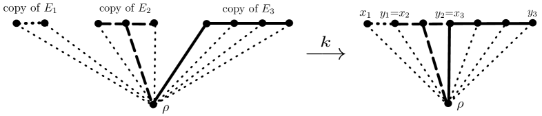
In order to apply Lemma 2.6, we separate vertices as follows: We consider the disjoint union $\Lambda^{\prime}$ of the sets $\Lambda_{E_{l}}\setminus\{\rho\}$ together will all vertices $i\in\Lambda$ which are in none of these sets. More formally, let $i^{l}$ denote the copy of $i\in\Lambda_{E_{l}}\setminus\{\rho\}$ corresponding to the subgraph $(\Lambda_{E_{l}},E_{l})$. Then, one has

$\displaystyle\Lambda^{\prime}=\{i^{l}:1\leq l\leq n,i\in\Lambda_{E_{l}}\setminus\{\rho\}\}\cup\{i\in\Lambda:i\notin\Lambda_{E_{l}}\text{ for all }1\leq l\leq n\}.$ (2.54)

Let $G^{\prime}=(\Lambda^{\prime}\cup\{\rho\},E^{\prime})$ be the corresponding complete graph and $k:\Lambda^{\prime}\cup\{\rho\}\to\Lambda\cup\{\rho\}$ be the natural map $i^{l}\mapsto i$ for $i\in\Lambda_{E_{l}}\setminus\{\rho\}$, $i\mapsto i$ for vertices not contained in any $\Lambda_{E_{l}}\setminus\{\rho\}$, and $\rho\mapsto\rho$, cf. Fig. 1.

Refer to caption

Figure 1: illustration of the map $k$

We endow the edges $e^{\prime}\in E^{\prime}$ with weights $W_{e^{\prime}}^{\prime}\geq 0$ as follows. For any edge $\{i,j\}\in E_{l}$ with $1\leq l\leq n$ and $\rho\notin\{i,j\}$, the corresponding edge $\{i^{l},j^{l}\}$ inherits its weight: $W_{i^{l}j^{l}}^{\prime}=W_{ij}$. Observe that a vertex $i\in\Lambda^{\prime}$ can be incident to edges in several $E_{l}$’s. For pinning edges $\{i,\rho\}$, we split the weight $W_{i\rho}$ as follows. In the case $\{i,\rho\}\in E_{l}$ for some $l$, we set $W_{i^{k}\rho}^{\prime}=(W_{i\rho}-\varepsilon)\delta_{kl}+\varepsilon/|\{l^{\prime}:i\in\Lambda_{E_{l^{\prime}}}\}|$, $1\leq k\leq n$; the index $l$ is unique since the $E_{l}$ are pairwise disjoint. In the case $\{i,\rho\}\notin E_{l}$ for all $l$, we set $W_{i^{k}\rho}^{\prime}=W_{i\rho}/|\{l:i\in\Lambda_{E_{l}}\}|$ for all $k$. Note that $\sum_{k=1}^{n}W_{i^{k}\rho}^{\prime}=W_{i\rho}$ and $W_{i^{k}\rho}^{\prime}\geq{\varepsilon}/n>0$ for all $k$ since $W_{i\rho}\geq{\varepsilon}$. For all other edges $e\in E^{\prime}$, we set $W_{e^{\prime}}^{\prime}=0$. For $1\leq l\leq n$, we set $e_{l}^{\prime}=\{x_{l}^{l},y_{l}^{l}\}\in E^{\prime}$ and $m_{e_{l}^{\prime}}^{\prime}=m_{e_{l}}$, but $m_{e^{\prime}}^{\prime}=0$ for all other edges $e^{\prime}\in E^{\prime}$. Then, Lemmas 2.6 and 2.8 and Remark 2.9 are applicable. In particular, on $U$ the bound $m_{e_{l}}\mathcal{R}^{G_{l}}(c,x_{l}\leftrightarrow y_{l})\leq 1-\theta$ and Remark 2.9 imply $m_{e_{l}}({\mathcal{G}}_{l})_{e_{l},e_{l}}\leq 1-\theta$ and then, by Lemma 2.8(b), $\sqrt{M_{l}}{\mathcal{G}}_{l}\sqrt{M_{l}}\leq(1-\theta)\operatorname{Id}$ for all $l$. As a consequence, by Lemma 2.8(a), $\sqrt{M^{\prime}}{\mathcal{G}}^{\prime}\sqrt{M^{\prime}}\leq(1-\theta)\operatorname{Id}$, which implies $\sqrt{M}{\mathcal{G}}\sqrt{M}\leq(1-\theta)\operatorname{Id}$ by Lemma 2.6. Note that this estimate is uniform in $\varepsilon>0$. Thus, by Lemma 2.4, Assumption 2.2 is satisfied, also in the limit $\varepsilon\to 0$. Combining formulas (2.31), (2.47), (2.48), and (2.51), we obtain

$\displaystyle\det(\operatorname{Id}-M{\mathcal{G}}(u,s))\geq$ $\displaystyle\det(\operatorname{Id}-M^{\prime}{\mathcal{G}}^{\prime}(u^{\prime},s^{\prime}))=\prod_{l=1}^{n}\det(\operatorname{Id}-M_{l}{\mathcal{G}}_{l})$
$\displaystyle=$ $\displaystyle\prod_{l=1}^{n}(1-m_{e_{l}}({\mathcal{G}}_{l})_{e_{l},e_{l}})\geq\prod_{l=1}^{n}(1-m_{e_{l}}\mathcal{R}^{G_{l}}(c,x_{l}\leftrightarrow y_{l})).$ (2.55)

Rayleigh’s monotonicity principle and its consequence (2.51) allow us to conclude.   

2.3 Proof of Theorem 1.3

In this section, we will prove Theorem 1.3. We consider the model described in Section 1.4 with $\alpha>3$, possibly extended by additional non-nearest neighbor edges $e$ with weights $W_{e}\geq 0$. Throughout this section, $N$ is fixed and hence, we drop the dependence on $N$ in the notation. The important point is that the final estimates are uniform in $N$.

Recall the notation $e=\{x_{e},y_{e}\}$ with $x_{e}<y_{e}$ for any edge $e$. We take a sequence of cutoff parameters $\delta_{l}$, $l\in{\mathbb{N}}$ and associate the $\delta_{l}$ to nearest-neighbor edges on ${\mathbb{N}}$ by setting $\delta_{\{l-1,l\}}:=\delta_{l}$ for $l\geq 2$. Remember that we defined $\chi_{ij}=\chi_{e}=1_{(-\infty,1+\delta_{e})}$ for $e=\{i,j\}$. For $i<j$, we set

$\displaystyle\overline{\chi}_{ij}:=\prod_{l=i+1}^{j}\chi_{l-1,l}(B_{l-1,l}).$ (2.56)
Lemma 2.11

Let $E^{\prime},E^{\prime\prime}\subseteq E_{N}$ be disjoint subsets of $E_{N}$, where every $e\in E^{\prime}$ is a nearest neighbor edge: $y_{e}-x_{e}=1$, and for any two different $e,\tilde{e}\in E^{\prime}\cup E^{\prime\prime}$ the open intervals $(x_{e},y_{e})$ and $(x_{\tilde{e}},y_{\tilde{e}})$ are disjoint. Assume that $\sum_{l=1}^{\infty}\sqrt{\delta_{l}}<\infty$ and set $C_{\delta}=e^{\sqrt{2}\sum_{l=1}^{\infty}\sqrt{\delta_{l}}}$, which is uniform in $N$. Then, for all exponents $m_{e}$ satisfying $0\leq m_{e}<W_{e}$ for $e\in E^{\prime}$ and $0\leq m_{e}<\left(C_{\delta}\sum_{i=x_{e}+1}^{y_{e}}\frac{1}{W_{i-1,i}}\right)^{-1}$ for $e\in E^{\prime\prime}$, we have

$\displaystyle{\mathbb{E}}_{W,h}^{[N]}\left[\prod_{e\in E^{\prime}}B_{e}^{m_{e}}\cdot\prod_{e\in E^{\prime\prime}}(B_{e}^{m_{e}}\overline{\chi}_{e})\right]\leq\prod_{e\in E^{\prime}}\frac{1}{1-\frac{m_{e}}{W_{e}}}\prod_{e\in E^{\prime\prime}}\frac{1}{1-C_{\delta}m_{e}\sum_{i=x_{e}+1}^{y_{e}}\frac{1}{W_{i-1,i}}}.$ (2.57)

Proof. We will show that Assumption 2.2 is satisfied and on the support of $\prod_{e\in E^{\prime\prime}}\overline{\chi}_{e}$, we have

$\displaystyle\det(\operatorname{Id}-M{\mathcal{G}})\geq\prod_{e\in E^{\prime}}\left(1-\frac{m_{e}}{W_{e}}\right)\prod_{e\in E^{\prime\prime}}\left(1-C_{\delta}m_{e}\sum_{i=x_{e}+1}^{y_{e}}\frac{1}{W_{i-1,i}}\right).$ (2.58)

It suffices to prove this in the case $W_{ij}=0$ for all edges $\{i,j\}$ with $|i-j|\geq 2$. The general case follows from Lemma 2.5. Using (2.58) and Lemma 2.3, we argue

$\displaystyle{\mathbb{E}}_{W,h}^{[N]}$ $\displaystyle\left[\prod_{e\in E^{\prime}}B_{e}^{m_{e}}\cdot\prod_{e\in E^{\prime\prime}}(B_{e}^{m_{e}}\overline{\chi}_{e})\right]={\mathbb{E}}_{W,h}^{[N]}\left[\prod_{e\in E^{\prime}}B_{e}^{m_{e}}\cdot\prod_{e\in E^{\prime\prime}}(B_{e}^{m_{e}}\overline{\chi}_{e})\frac{\det(\operatorname{Id}-M{\mathcal{G}})}{\det(\operatorname{Id}-M{\mathcal{G}})}\right]$
$\displaystyle\leq$ $\displaystyle\frac{{\mathbb{E}}_{W,h}^{[N]}\left[\prod_{e\in E^{\prime}}B_{e}^{m_{e}}\cdot\prod_{e\in E^{\prime\prime}}(B_{e}^{m_{e}}\overline{\chi}_{e})\det(\operatorname{Id}-M{\mathcal{G}})\right]}{\prod_{e\in E^{\prime}}\left(1-\frac{m_{e}}{W_{e}}\right)\prod_{e\in E^{\prime\prime}}\left(1-C_{\delta}m_{e}\sum_{i=x_{e}+1}^{y_{e}}\frac{1}{W_{i-1,i}}\right)}$
$\displaystyle\leq$ $\displaystyle\prod_{e\in E^{\prime}}\frac{1}{1-\frac{m_{e}}{W_{e}}}\prod_{e\in E^{\prime\prime}}\frac{1}{1-C_{\delta}m_{e}\sum_{i=x_{e}+1}^{y_{e}}\frac{1}{W_{i-1,i}}},$ (2.59)

which concludes the proof.

To prove (2.58), we apply Theorem 2.10 as follows. For $e\in E^{\prime}\cup E^{\prime\prime}$, we consider the pairwise disjoint sets of edges $E_{e}=\{\{i-1,i\}:\,x_{e}<i\leq y_{e}\}$ and the corresponding graphs $G_{e}=(\{x_{e},\ldots,y_{e}\},E_{e})$. In particular, $E_{e}=\{e\}$ for $e\in E^{\prime}$. We claim that

$\displaystyle m_{e}\mathcal{R}^{G_{e}}(c,x_{e}\leftrightarrow y_{e})<1\quad\text{ for }e\in E^{\prime}\cup E^{\prime\prime}$ (2.60)

holds on $U\subseteq\operatorname{supp}\prod_{e\in E^{\prime\prime}}\overline{\chi}_{e}$, cf. formula (2.9). Indeed, for the nearest-neighbor edges $e\in E^{\prime}$, we have

$\displaystyle m_{e}\mathcal{R}^{G_{e}}(c,x_{e}\leftrightarrow y_{e})=$ $\displaystyle\frac{m_{e}}{c_{e}}=\frac{m_{e}e^{u_{x_{e}}+u_{y_{e}}}}{W_{e}e^{u_{x_{e}}+u_{y_{e}}}B_{e}}\leq\frac{m_{e}}{W_{e}}<1.$ (2.61)

For edges $e\in E^{\prime\prime}$, we will show

$\displaystyle m_{e}\mathcal{R}^{G_{e}}(c,x_{e}\leftrightarrow y_{e})\leq m_{e}C_{\delta}\sum_{i=x_{e}+1}^{y_{e}}\frac{1}{W_{i-1,i}}<1.$ (2.62)

The inequalities “$<1$” in (2.61) and (2.62) follow from the assumptions on $m_{e}$. Therefore, by Theorem 2.10, Assumption 2.2 is valid and we have

$\displaystyle\det(\operatorname{Id}-M{\mathcal{G}})\geq\prod_{e\in E^{\prime}\cup E^{\prime\prime}}(1-m_{e}\mathcal{R}^{G_{e}}(c,x_{e}\leftrightarrow y_{e})).$ (2.63)

Inserting the bounds (2.61) and (2.62), we obtain (2.58).

Finally we prove (2.62). Consider an edge $e\in E^{\prime\prime}$. Using the definition (2.49) of the conductances $c_{e}$ and the series law for the resistances between $x_{e}$ and $y_{e}$, we obtain

$\displaystyle\mathcal{R}^{G_{e}}(c,x_{e}\leftrightarrow y_{e})$ $\displaystyle=\sum_{i=x_{e}+1}^{y_{e}}\frac{1}{c_{i-1,i}}=\sum_{i=x_{e}+1}^{y_{e}}\frac{e^{u_{x_{e}}+u_{y_{e}}}}{W_{i-1,i}e^{u_{i-1}+u_{i}}B_{e}}$
$\displaystyle\leq\sum_{i=x_{e}+1}^{y_{e}}\frac{e^{u_{x_{e}}-u_{i-1}+u_{y_{e}}-u_{i}}}{W_{i-1,i}},$ (2.64)

where we used $B_{e}\geq 1$. On the support of $\overline{\chi}_{e}$, one has for all $l\in\{x_{e}+1,\ldots,y_{e}\}$,

$\displaystyle 1+\delta_{l}>B_{l-1,l}\geq\cosh(u_{l-1}-u_{l})\geq 1+\frac{1}{2}(u_{l-1}-u_{l})^{2}$ (2.65)

and hence $|u_{l-1}-u_{l}|\leq\sqrt{2\delta_{l}}$. For $i=x_{e}+1,\ldots,y_{e}$, we estimate

$\displaystyle u_{x_{e}}-u_{i-1}+u_{y_{e}}-u_{i}\leq\sum_{\begin{subarray}{c}l=x_{e}+1\\ l\neq i\end{subarray}}^{y_{e}}|u_{l-1}-u_{l}|\leq\sqrt{2}\sum_{\begin{subarray}{c}l=x_{e}+1\\ l\neq i\end{subarray}}^{y_{e}}\sqrt{\delta_{l}}\leq\log C_{\delta}.$ (2.66)

Inserting this in (2.64) concludes the proof of (2.62).   

Using Lemma 2.11, we prove now the bounds in the inhomogeneous one-dimensional model.

Proof of Theorem 1.3. We start with a pointwise bound on each factor $B_{e}^{m_{e}}$ corresponding to an edge $e\in E^{\prime\prime}$. For this purpose, keeping $e$ fixed for the moment, we abbreviate $x=x_{e}$, $y=y_{e}\geq x_{e}+1$ and $m=m_{e}\geq 0$. We consider the partition of unity (cf. Fig. 2)

Refer to caption

Figure 2: cut-off functions used in the partition of unity
$\displaystyle 1=\overline{\chi}_{xy}+(1-\overline{\chi}_{xy})=\overline{\chi}_{xy}+\sum_{j=x+1}^{y}\chi^{c}_{j-1,j}\overline{\chi}_{j,y}\text{ with }\chi^{c}_{j-1,j}:=1-\chi_{j-1,j}(B_{j-1,j}),$ (2.67)

where the constants $\delta_{j}$ appearing in the definition $\chi_{j-1,j}(B)=1_{\{B<1+\delta_{j}\}}$ will be specified later. This means that either all nearest-neighbor pairs between $x$ and $y$ are protected in the sense that the factor $\chi_{j-1,j}$ of the corresponding edge is present or there is a largest index $j$ for which the edge $\{j-1,j\}$ is unprotected. We estimate the $j$-th summand in the last sum, using

$\displaystyle\chi_{j-1,j}^{c}=1_{\{B_{j-1,j}\geq 1+\delta_{j}\}}\leq\left(\frac{B_{j-1,j}}{1+\delta_{j}}\right)^{p_{j}}$ (2.68)

where $p_{j}>0$ will be also chosen later. Inserting this bound and multiplying with $B_{e}^{m}=B_{xy}^{m}$ yields

$\displaystyle B_{e}^{m}\leq B_{xy}^{m}\overline{\chi}_{xy}+\sum_{j=x+1}^{y}(1+\delta_{j})^{-p_{j}}B_{xy}^{m}B_{j-1,j}^{p_{j}}\overline{\chi}_{j,y}.$ (2.69)

We estimate $B_{xy}$ in the $j$-th summand as follows. By [DSZ10, Lemma 2 in Section 5.2], one has $B_{ij}\leq 2B_{ik}B_{kj}$ for all $i,j,k$. Given $j$ with $x+1\leq j\leq y$, this yields

$\displaystyle B_{xy}\leq 2^{j-x}B_{jy}\prod_{i=x+1}^{j}B_{i-1,i},$ (2.70)

with the convention $B_{yy}=1$. Inserting this in the $j$-th summand in (2.69), we obtain

$\displaystyle B_{xy}^{m}\leq B_{xy}^{m}\overline{\chi}_{xy}+\sum_{j=x+1}^{y}\frac{2^{(j-x)m}}{(1+\delta_{j})^{p_{j}}}\left(\prod_{i=x+1}^{j-1}B_{i-1,i}^{m}\right)B_{j-1,j}^{m+p_{j}}B_{jy}^{m}\overline{\chi}_{jy}.$ (2.71)

We now take the product of both sides of this inequality over $e=\{x_{e},y_{e}\}\in E^{\prime\prime}$, not suppressing the $e$-dependence in the notation anymore, and expand the product of sums on the r.h.s. in a sum of products. To keep the calculations readable, we introduce some abbreviations, locally for this proof. Let $X_{e,j}=\frac{2^{(j-x)m}}{(1+\delta_{j})^{p_{j}}}\left(\prod_{i=x+1}^{j-1}B_{i-1,i}^{m}\right)B_{j-1,j}^{m+p_{j}}B_{jy}^{m}\overline{\chi}_{jy}$, $j\in\{x_{e}+1,\ldots,y_{e}\}$, denote the summand on the r.h.s. of (2.71) indexed by $j$, and $X_{e,x_{e}}=B_{x_{e}y_{e}}^{m_{e}}\overline{\chi}_{x_{e}y_{e}}$ the first summand. We obtain

$\displaystyle\prod_{e\in E^{\prime\prime}}B_{x_{e}y_{e}}^{m_{e}}\leq\prod_{e\in E^{\prime\prime}}\sum_{j=x_{e}}^{y_{e}}X_{e,j}=\sum_{(j_{e})_{e\in E^{\prime\prime}}\in\mathcal{I}}\prod_{e\in E^{\prime\prime}}X_{e,j_{e}}$ (2.72)

with the cartesian product $\mathcal{I}=\prod_{e\in E^{\prime\prime}}\{x_{e},\ldots,y_{e}\}$. Therefore,

$\displaystyle{\mathbb{E}}\left[\prod_{e\in E^{\prime}}B_{x_{e}y_{e}}^{m_{e}}\cdot\prod_{e\in E^{\prime\prime}}B_{x_{e}y_{e}}^{m_{e}}\right]\leq\sum_{(j_{e})_{e\in E^{\prime\prime}}\in\mathcal{I}}{\mathbb{E}}\left[\prod_{e\in E^{\prime}}B_{x_{e}y_{e}}^{m_{e}}\cdot\prod_{e\in E^{\prime\prime}}X_{e,j_{e}}\right].$ (2.73)

We will estimate the expectations in the sum using Lemma 2.11 showing that it is applicable for an appropriate choice of $\delta_{j}$ and $p_{j}$. We illustrate first the strategy in two special cases. In the special case that $E^{\prime}$ consists of a single edge $e=\{x_{e},y_{e}\}$ and $E^{\prime\prime}=\emptyset$, Lemma 2.11 gives

$\displaystyle{\mathbb{E}}\left[B_{x_{e}y_{e}}^{m_{e}}\right]\leq\frac{1}{1-\frac{m_{e}}{W_{e}}}=:Y_{e}$ (2.74)

because $m_{e}<W_{e}$. Similarly, if $E^{\prime}=\emptyset$ and $E^{\prime\prime}$ consists of a single edge $e=\{x_{e},y_{e}\}$, Lemma 2.11 will give us

$\displaystyle{\mathbb{E}}\left[X_{e,x_{e}}\right]={\mathbb{E}}\left[B_{x_{e}y_{e}}^{m_{e}}\overline{\chi}_{x_{e}y_{e}}\right]\leq\frac{1}{1-C_{\delta}m_{e}\sum_{k=x_{e}+1}^{y_{e}}\frac{1}{W_{k-1,k}}}=:Y_{e,x_{e}}$ (2.75)

and for $j\in\{x_{e}+1,\ldots,y_{e}\}$

$\displaystyle{\mathbb{E}}\left[X_{e,j}\right]=\frac{2^{(j-x_{e})m_{e}}}{(1+\delta_{j})^{p_{j}}}{\mathbb{E}}\left[\left(\prod_{i=x_{e}+1}^{j-1}B_{i-1,i}^{m_{e}}\right)B_{j-1,j}^{m_{e}+p_{j}}B_{jy_{e}}^{m_{e}}\overline{\chi}_{jy_{e}}\right]$
$\displaystyle\leq\frac{2^{(j-x_{e})m_{e}}}{(1+\delta_{j})^{p_{j}}}\prod_{i=x_{e}+1}^{j-1}\frac{1}{1-\frac{m_{e}}{W_{i-1,i}}}\cdot\frac{1}{1-\frac{m_{e}+p_{j}}{W_{j-1,j}}}\cdot\frac{1}{1-C_{\delta}m_{e}\sum_{k=j+1}^{y_{e}}\frac{1}{W_{k-1,k}}}=:Y_{e,j}.$ (2.76)

In the general case, Lemma 2.11 will give

$\displaystyle{\mathbb{E}}\left[\prod_{e\in E^{\prime}}B_{x_{e}y_{e}}^{m_{e}}\cdot\prod_{e\in E^{\prime\prime}}X_{e,j_{e}}\right]\leq\prod_{e\in E^{\prime}}Y_{e}\cdot\prod_{e\in E^{\prime\prime}}Y_{e,j_{e}}$ (2.77)

for all $(j_{e})_{e\in E^{\prime\prime}}\in\mathcal{I}$. Summing over $\mathcal{I}$ and recombining the sum over products to a product of sums, we obtain

$\displaystyle{\mathbb{E}}\left[\prod_{e\in E^{\prime}\cup E^{\prime\prime}}B_{x_{e}y_{e}}^{m_{e}}\right]\leq\sum_{(j_{e})_{e\in E^{\prime\prime}}\in\mathcal{I}}\prod_{e\in E^{\prime}}Y_{e}\cdot\prod_{e\in E^{\prime\prime}}Y_{e,j_{e}}=\prod_{e\in E^{\prime}}Y_{e}\cdot\prod_{e\in E^{\prime\prime}}\sum_{j=x_{e}}^{y_{e}}Y_{e,j}.$ (2.78)

To check applicability of Lemma 2.11, we need $\delta_{j}$ and $p_{j}$ such that $\sum_{l=1}^{\infty}\sqrt{\delta_{l}}<\infty$ and all denominators in the $Y$-factors are strictly positive. For later use, some estimates will be sharper than needed at this point.

Recall the assumption on the weights $W_{j-1,j}\geq\overline{W}j^{\alpha}$ with $\alpha>3$. Let $\kappa\in(0,1]$ and $\gamma\geq 0$ with $\alpha-\gamma>3$ be given. We set $\delta_{j}:=j^{-(\alpha-\gamma-1)}$ for $j\in{\mathbb{N}}$. With this choice, we have

$\displaystyle\sum_{l=1}^{\infty}\sqrt{\delta_{l}}=1+\sum_{l=2}^{\infty}l^{-\frac{\alpha-\gamma-1}{2}}\leq 1+\int_{1}^{\infty}t^{-\frac{\alpha-\gamma-1}{2}}\,dt=\frac{\alpha-\gamma-1}{\alpha-\gamma-3}<\infty.$ (2.79)

We take now $c_{3},{c_{4}},{\overline{W}_{0}}$ as in (1.22) and (1.23) and $\overline{W}\geq{\overline{W}_{0}}$. For a given $e=\{x,y\}\in E^{\prime\prime}$, we consider $Y_{e,j}$ with $x\leq j\leq y$, suppressing the $e$-dependence again in the notation. We need to estimate $m/W_{i-1,i}$ for $x<i<y$, $(m+p_{j})/W_{j-1,j}$ for $x<j\leq y$, and $C_{\delta}m\sum_{k=j+1}^{y}\frac{1}{W_{k-1,k}}$ for $x\leq j\leq y$. Recall that $m_{x}=c_{3}\overline{W}x^{\gamma}={c_{4}}\overline{W}x^{\gamma}/\log 2$ and let $m\in[0,m_{x}]$. For all $i\geq x$, using $\gamma-\alpha<0$ and $c_{3}\leq(16\log 2)^{-1}\leq\frac{1}{4}$, we estimate

$\displaystyle\frac{m}{W_{i-1,i}}\leq\frac{m_{x}}{\overline{W}i^{\alpha}}=c_{3}x^{\gamma}i^{-\alpha}\leq c_{3}x^{\gamma-\alpha}\leq c_{3}\leq\frac{1}{4}.$ (2.80)

For $j\in{\mathbb{N}}$, we set $p_{j}:=4{c_{4}}\overline{W}j^{\alpha}$. For $x<j\leq y$, we obtain with ${c_{4}}\leq\frac{1}{16}$ the bound

$\displaystyle\frac{m+p_{j}}{W_{j-1,j}}\leq\frac{1}{4}+\frac{p_{j}}{W_{j-1,j}}\leq\frac{1}{4}+\frac{p_{j}}{\overline{W}j^{\alpha}}=\frac{1}{4}+4{c_{4}}\leq\frac{1}{2}.$ (2.81)

Finally, for $x\leq j\leq y$, we estimate, using $\alpha>3$,

$\displaystyle\sum_{k=j+1}^{y}\frac{1}{W_{k-1,k}}\leq\sum_{k=j+1}^{y}\frac{1}{\overline{W}k^{\alpha}}\leq\int_{x}^{\infty}\frac{1}{\overline{W}t^{\alpha}}\,dt=\frac{x^{1-\alpha}}{\overline{W}(\alpha-1)}\leq\frac{x^{1-\alpha}}{2\overline{W}}.$ (2.82)

Because of (2.79), the constant $C_{\delta}$ from Lemma 2.11 satisfies $1\leq C_{\delta}=e^{\sqrt{2}\sum_{l=1}^{\infty}\sqrt{\delta_{l}}}\leq e^{\sqrt{2}\frac{\alpha-\gamma-1}{\alpha-\gamma-3}}$. Hence, our choice of $c_{3}$ in (1.22) and (1.23) yields $c_{3}\leq\frac{2}{3}\kappa/C_{\delta}$. Together with (2.82), using $\gamma+1-\alpha<0$, it follows

$\displaystyle C_{\delta}m\sum_{k=j+1}^{y}\frac{1}{W_{k-1,k}}\leq C_{\delta}m_{x}\frac{x^{1-\alpha}}{2\overline{W}}=\frac{C_{\delta}c_{3}x^{\gamma+1-\alpha}}{2}\leq\frac{C_{\delta}c_{3}}{2}\leq\frac{\kappa}{3}<1.$ (2.83)

This shows that the assumptions of Lemma 2.11 needed above are fulfilled.

We now use the estimates above to bound the $Y$-variables defined in (2.75) and (2.76). Using $\kappa\in(0,1]$, one has $(1-t)^{-1}\leq 1+\kappa/2$ for all $t\in[0,\kappa/3]$. Consequently, (2.83) implies

$\displaystyle\frac{1}{1-C_{\delta}m\sum_{k=j+1}^{y}\frac{1}{W_{k-1,k}}}\leq 1+\frac{\kappa}{2}\leq 2\text{ for }x\leq j\leq y.$ (2.84)

In the case $j=x$, this yields

$\displaystyle Y_{e,x}\leq 1+\frac{\kappa}{2}.$ (2.85)

We consider now $x<j\leq y$. For $t\in[0,\frac{1}{2}]$, we have $(1-t)^{-1}\leq\min\{2,e^{2t}\}$. We apply this estimate to $t=\frac{m_{e}}{W_{i-1,i}}\leq\frac{1}{4}$, cf. (2.80), with $x<i<j$ and to $t=\frac{m+p_{j}}{W_{j-1,j}}\leq\frac{1}{2}$, cf. (2.81), to obtain, using (2.83) and $C_{\delta}\geq 1$,

$\displaystyle\prod_{i=x+1}^{j-1}\!\!\frac{1}{1-\frac{m_{e}}{W_{i-1,i}}}\cdot\frac{1}{1-\frac{m_{e}+p_{j}}{W_{j-1,j}}}\leq 2\!\!\prod_{i=x+1}^{j-1}\!\!e^{2\frac{m}{W_{i-1,i}}}\leq 2e^{2m\sum_{i=x+1}^{y-1}\frac{1}{W_{i-1,i}}}\leq 2e^{2\kappa/3}\leq 2e.$ (2.86)

Substituting this and (2.84) in the definition (2.76) of $Y_{e,j}$, it follows, using in addition $\log(1+\delta_{j})\geq\delta_{j}/2$ since $\delta_{j}=j^{-(\alpha-\gamma-1)}\in[0,1]$,

$\displaystyle Y_{e,j}$ $\displaystyle\leq 4e\frac{2^{(j-x)m}}{(1+\delta_{j})^{p_{j}}}=4e\cdot e^{(j-x)m\log 2-p_{j}\log(1+\delta_{j})}\leq 4e\cdot e^{(j-x)m\log 2-\frac{1}{2}p_{j}\delta_{j}}$
$\displaystyle\leq 4e\cdot e^{jm_{x}\log 2-\frac{1}{2}p_{j}\delta_{j}}=4e\cdot e^{{c_{4}}\overline{W}x^{\gamma}j-2{c_{4}}\overline{W}j^{\gamma+1}}\leq 4e\cdot e^{-{c_{4}}\overline{W}j^{\gamma+1}}\leq 4e\cdot e^{-{c_{4}}\overline{W}j},$ (2.87)

where we used $x\leq j$ and $\gamma\geq 0$ in the last two inequalities, respectively. Summing this bound over $j=x+1,\ldots,y$ and adding the bound (2.85) for $Y_{e,x}$ yields

$\displaystyle\sum_{j=x}^{y}Y_{e,j}\leq 1+\frac{\kappa}{2}+4e\sum_{j=x+1}^{y}e^{-{c_{4}}\overline{W}j}\leq 1+\frac{\kappa}{2}+4e\frac{e^{-{c_{4}}\overline{W}(x+1)}}{1-e^{-{c_{4}}\overline{W}}}.$ (2.88)

Using $\overline{W}\geq{\overline{W}_{0}}$ and our choice (1.22) of ${\overline{W}_{0}}$, we observe $e^{-{c_{4}}\overline{W}}\leq\sqrt{\kappa}/6$. Together with $x\geq 1$ and $\kappa\leq 1$ this yields

$\displaystyle 4e\frac{e^{-{c_{4}}\overline{W}(x+1)}}{1-e^{-{c_{4}}\overline{W}}}\leq 4e\frac{e^{-2{c_{4}}\overline{W}}}{1-e^{-{c_{4}}\overline{W}}}\leq 4e\frac{\left(\frac{\sqrt{\kappa}}{6}\right)^{2}}{1-\frac{1}{6}}=\frac{2e}{15}\kappa\leq\frac{\kappa}{2}.$ (2.89)

We conclude $\sum_{j=x}^{y}Y_{e,j}\leq 1+\kappa$. Substituting this bound and the definition (2.74) of $Y_{e}$ in (2.78), we conclude

$\displaystyle{\mathbb{E}}\left[\prod_{e\in E^{\prime}\cup E^{\prime\prime}}B_{x_{e}y_{e}}^{m_{e}}\right]\leq\prod_{e\in E^{\prime}}Y_{e}\cdot\prod_{e\in E^{\prime\prime}}\sum_{j=x_{e}}^{y_{e}}Y_{e,j}\leq(1+\kappa)^{|E^{\prime\prime}|}\prod_{e\in E^{\prime}}\frac{1}{1-\frac{m_{e}}{W_{e}}}.$ (2.90)

This proves the first inequality in claim (1.20). The second inequality in this claim follows from the bound $(1-\frac{m_{e}}{W_{e}})^{-1}\leq 1+\kappa$. Finally, (1.21) follows from (1.20) and $\cosh(u_{x}-u_{y})\leq B_{e}$, which is a consequence of definition (1.4).   

We conclude this section with the proof of the quantitative version of Theorem 1.3.

Proof of Lemma 1.4. In the proof of Theorem 1.3, we showed that ${\overline{W}_{0}}$, $c_{3}$, and ${c_{4}}$ can be chosen as in (1.22) and (1.23). For $\kappa=1$, we obtain ${\overline{W}_{0}}=\log 6/{c_{4}}$, which yields the expression in (1.24).   

3 Bounds in the hierarchical and long-range model

3.1 Bounds in the hierarchical model

Proof of Theorem 1.2. As described in the proof of Theorem 3.2 in [DMR24], $u_{i}$, $i\in\Lambda_{N}$, are identically distributed and by [DMR22, Corollary 2.3] the law of $u_{i_{1}}$ with $i_{1}:=(0,\ldots,0)\in\{0,1\}^{N}$ agrees with the law of $u_{i_{1}}$ in an effective model on the complete graph with vertex set $A=\{j,i_{1},\ldots,i_{N}\}$, weights $W_{i_{l-1},i_{l}}=2^{2l-3}w^{H}(l)$, and pinnings $h_{i_{l}}:=2^{l-1}h^{H}$, $2\leq l\leq N$, $h_{i_{1}}:=h^{H}$. The other weights also need to have specific values in this effective model, but they are not displayed here because these values do not play any role in the subsequent arguments. The mentioned coincidence of laws implies

$\displaystyle{\mathbb{E}}_{W^{H},h^{H}}^{\Lambda_{N}}[(\cosh u_{i_{1}})^{m}]={\mathbb{E}}_{W,h}^{A}[(\cosh u_{i_{1}})^{m}]={\mathbb{E}}_{W,h}^{A}[(\cosh(u_{i_{1}}-u_{\rho}))^{m}],$ (3.1)

where in the last step we used $u_{\rho}=0$. We regard the pinning point $\rho$ as an additional vertex at the end of the antichain $j,i_{1},\ldots,i_{N}$, writing $i_{N+1}:=\rho$. Note that by assumption (1.18), one has $W_{i_{l-1}i_{l}}=2^{2l-3}w^{H}(l)\geq\overline{W}l^{\alpha}$ for $l\in\{2,\ldots,N\}$ and $W_{i_{N},i_{N+1}}=h_{i_{N}}=2^{N-1}h^{H}\geq\overline{W}(N+1)^{\alpha}$. Hence, we can apply the bound (1.21) in Theorem 1.3 for $x=i_{1}$, $y=i_{N+1}$, and case P2 which gives claim (1.19).

Recall that ${c_{1}}=\frac{2}{3}e^{-\sqrt{2}\frac{\alpha-1}{\alpha-3}}$; cf. its definition in Theorem 1.1. Taking $\gamma=0$ in (1.22) and (1.23) and using $\kappa\leq(16{c_{1}}\log 2)^{-1}$ from (1.14) yields

$\displaystyle c_{3}=$ $\displaystyle c_{3}(\kappa,\alpha)=\min\left\{\frac{2}{3}\kappa e^{-\sqrt{2}\frac{\alpha-1}{\alpha-3}},\frac{1}{16\log 2}\right\}={c_{1}}\kappa,$ (3.2)
$\displaystyle{\overline{W}_{0}}=$ $\displaystyle{\overline{W}_{0}}(\kappa,\alpha,\gamma)=\frac{1}{2c_{3}}\log_{2}\frac{36}{\kappa}=\frac{1}{2{c_{1}}\kappa}\log_{2}\frac{36}{\kappa}.$ (3.3)

Hence, by (1.14), the assumptions $\overline{W}\geq{\overline{W}_{0}}$ and $0\leq m\leq c_{3}\overline{W}$ of Theorem 1.3 are satisfied.

We treat now the two examples from Theorem 1.1, which are referred to in Theorem 1.2. For the first example, let $s\in(0,1)$ and $\kappa=\overline{W}^{-s}$. For $\overline{W}$ large enough, depending on $\alpha$ and $s$, one has $\kappa\leq(16{c_{1}}\log 2)^{-1}$ and $\frac{1}{2{c_{1}}}\frac{1}{\kappa}\log_{2}\frac{36}{\kappa}=\frac{1}{2{c_{1}}}\overline{W}^{s}\log_{2}(36\overline{W}^{s})\leq\overline{W}$.

For the second example, let $\kappa={c_{2}}\frac{\log\overline{W}}{\overline{W}}$ with ${c_{2}}>1/(2{c_{1}}\log 2)$. For $\overline{W}$ large enough, depending on $\alpha$, it follows $\kappa\leq(16{c_{1}}\log 2)^{-1}$ and

$\displaystyle\frac{1}{2{c_{1}}}\frac{1}{\kappa}\log_{2}\frac{36}{\kappa}=\frac{1}{2{c_{1}}{c_{2}}\log 2}\overline{W}\left(1+\frac{\log 36-\log{c_{2}}-\log\log\overline{W}}{\log\overline{W}}\right)\leq\overline{W}.$ (3.4)

Thus, the conditions in (1.14) are satisfied in both cases.   

Corollary 3.1

Under the assumptions of Theorem 1.2, for $\kappa,\overline{W},m$ as in Theorem 1.2, and for all $i,j\in\Lambda_{N}$, one has

$\displaystyle{\mathbb{E}}_{W^{H},h^{H}}^{\Lambda_{N}}[(\cosh(u_{i}-u_{j}))^{m/2}]\leq 2^{m/2}(1+\kappa).$ (3.5)

Proof. We observe that $\cosh(u_{i}-u_{j})\leq 2\cosh u_{i}\cosh u_{j}$. Applying first Cauchy-Schwarz and then (1.19), we deduce (3.5) as follows:

$\displaystyle{\mathbb{E}}_{W^{H},h^{H}}^{\Lambda_{N}}$ $\displaystyle[(\cosh(u_{i}-u_{j}))^{m/2}]\leq 2^{m/2}{\mathbb{E}}_{W^{H},h^{H}}^{\Lambda_{N}}[(\cosh u_{i})^{m/2}(\cosh u_{j})^{m/2}]$
$\displaystyle\leq 2^{m/2}{\mathbb{E}}_{W^{H},h^{H}}^{\Lambda_{N}}[(\cosh u_{i})^{m}]^{1/2}{\mathbb{E}}_{W^{H},h^{H}}^{\Lambda_{N}}[(\cosh u_{j})^{m}]^{1/2}\leq 2^{m/2}(1+\kappa).$ (3.6)


Remark.

It is straightforward to show the analogue result for the long-range Euclidean model. In the hierarchical model, one could even get rid of the factor $2^{m/2}$ in (3.5) by connecting the vertices $i$ and $j$ by an antichain going twice over all levels below the least common ancestor in the binary tree. This antichain is described in Remark 4.2 and visualized in Figure 4.3 in [DMR22]. As a result, one obtains a one-dimensional effective model with nearest-neighbor weights that increase up to the middle and decrease afterwards. The strategy of the proof of Theorem 1.2 can be adapted to this case. However, we do not know how to transfer this improvement to the long-range Euclidean model because Poudevigne’s monotonicity result [PA24, Theorem 6] is not applicable to $(\cosh(u_{i}-u_{j}))^{m/2}$ as it is to $(\cosh u_{i})^{m}$.

3.2 Bounds in the long-range model

The proof of Theorem 1.1 follows the lines of the proof of [DMR24, Theorem 1.4] up to minor modifications. To improve readability of this paper, we repeat the argument.

As in [DMR24], we use a comparison with a hierarchical $H^{2|2}$ model. Let $d\geq 1$ and $N\in{\mathbb{N}}$ and consider the box $\Lambda_{N}:=\{0,1,\ldots,2^{N}-1\}^{d}$. We use the bijection between $\Lambda_{N}$ with $\{0,1\}^{Nd}$ given by

$\displaystyle\phi:\Lambda_{N}\to\{0,1\}^{Nd},\quad\phi(i_{0},\ldots,i_{d-1})=(z_{0},\ldots,z_{Nd-1})$ (3.7)

with $z_{n}\in\{0,1\}$ the $\lfloor n/d\rfloor$-th digit in the binary expansion $i_{l}=\sum_{k=0}^{N-1}z_{dk+l}2^{k}$ and $l=n\,\mod\,d$. One may interpret the elements of $\{0,1\}^{Nd}$ as the leaves of a binary tree. Using this interpretation, for $z,z^{\prime}\in\{0,1\}^{Nd}$, the hierarchical distance $d_{H}(z,z^{\prime})$ equals the distance to the least common ancestor in the binary tree or equivalently

$\displaystyle d_{H}(z,z^{\prime})=\min(\{n\in\{0,\ldots,Nd-1\}:\,z_{m}=z_{m}^{\prime}\text{ for all }m\geq n\}\cup\{Nd\}).$ (3.8)

Proof of Theorem 1.1. Note that ${c_{1}}\kappa\overline{W}\geq-\log_{2}(\kappa/36)/2\geq\log_{2}6>1$ and hence there is some $m\geq 1$ fulfilling (1.14). Since ${\mathbb{E}}^{\Lambda_{N}}_{W,h}\left[(\cosh u_{i})^{m}\right]$ is increasing in $m$, it suffices to prove the claim for $m\geq 1$. We consider the long-range model described in Section 1.2 on the box $\Lambda_{N}$ with wired boundary with long-range weights $W^{+}_{ij}:=W_{ij}=w(\|i-j\|_{\infty})$ and pinning $h^{+}_{j}:=h_{j}$ given in (1.13). We compare it with a hierarchical model defined on the same box with the weights

$\displaystyle W^{-}_{ij}:=W^{H}_{ij}=w^{H}(d_{H}(\phi(i),\phi(j)))\text{ with }w^{H}(r):=w(2^{\lceil r/d\rceil})$ (3.9)

and uniform pinning given by $h^{-}:=h^{H}:=\min_{j\in\Lambda_{N}}h_{j}$. [DMR24, Lemma 3.4] states that $2^{\lceil d_{H}(\phi(i),\phi(j))/d\rceil}>\|i-j\|_{\infty}$ for all $i,j\in\Lambda_{N}$. Using that $w$ is monotonically decreasing, it follows that

$\displaystyle W_{ij}=w(\|i-j\|_{\infty})\geq w\left(2^{\lceil d_{H}(\phi(i),\phi(j))/d\rceil}\right)=W^{H}_{ij},\quad h_{i}\geq h^{H},$ (3.10)

for $i,j\in\Lambda_{N}$. Since $(\cosh u_{i})^{m}$ is a convex function of $e^{u_{i}}$ whenever $m\geq 1$, [PA24, Theorem 6] yields

$\displaystyle{\mathbb{E}}^{\Lambda_{N}}_{W,h}\left[(\cosh u_{i})^{m}\right]\leq{\mathbb{E}}^{\Lambda_{N}}_{W^{H},h^{H}}\left[(\cosh u_{i})^{m}\right]$ (3.11)

for all $i\in\Lambda_{N}$. Using the bijection $\phi:\Lambda_{N}\to\{0,1\}^{Nd}$ from (3.7), we identify $\Lambda_{N}$ with $\{0,1\}^{Nd}$. This yields the hierarchical model from Section 1.3 with $N$ replaced by $Nd$. In order to apply Theorem 1.2 we estimate the weights using the lower bound (1.12) for $w$

$\displaystyle w^{H}(r)=$ $\displaystyle w(2^{\lceil r/d\rceil})\geq 8\overline{W}2^{2d}\frac{(d\lceil r/d\rceil)^{\alpha}}{2^{2d\lceil r/d\rceil}}\geq 8\overline{W}2^{2d}\frac{r^{\alpha}}{2^{2d(1+r/d)}}=8\overline{W}2^{-2r}r^{\alpha}.$ (3.12)

In the following estimate, the first inequality is analogous to [DMR24, (3.22) and (3.23)], and the second inequality uses again the lower bound (1.12) for $w$. We find

$\displaystyle h^{H}\geq 2^{(N+1)d}w(2^{N+1})\geq 2^{(N+1)d}\cdot 8\overline{W}2^{2d}\frac{(Nd+d)^{\alpha}}{2^{2(N+1)d}}\geq 2\overline{W}2^{-Nd}(Nd+1)^{\alpha}.$ (3.13)

Note that we have dropped a factor $2^{2+d}$ in the last inequality. This verifies assumption (1.18) of Theorem 1.2 with $N$ substituted by $Nd$ and concludes the proof.   

Acknowledgement. This work was supported by the Deutsche Forschungsgemeinschaft (DFG, German Research Foundation) priority program SPP 2265 Random Geometric Systems and partly funded by DFG – Germany’s Excellence Strategy - GZ 2047/1, projekt-id 390685813. M.D. acknowledges the hospitality of the Newton Institute in Cambridge, where part of this work has been carried out.

References

  • [BCHS21] R. Bauerschmidt, N. Crawford, T. Helmuth, and A. Swan. Random spanning forests and hyperbolic symmetry. Comm. Math. Phys., 381(3):1223–1261, 2021.
  • [BH21] R. Bauerschmidt and T. Helmuth. Spin systems with hyperbolic symmetry: a survey. Proceedings of the ICM 2022, arXiv:2109.02566, 2021.
  • [BHS19] R. Bauerschmidt, T. Helmuth, and A. Swan. Dynkin isomorphism and Mermin-Wagner theorems for hyperbolic sigma models and recurrence of the two-dimensional vertex-reinforced jump process. Ann. Probab., 47(5):3375–3396, 2019.
  • [BHS21] R. Bauerschmidt, T. Helmuth, and A. Swan. The geometry of random walk isomorphism theorems. Ann. Inst. Henri Poincaré Probab. Stat., 57(1):408–454, 2021.
  • [Cra21] N. Crawford. Supersymmetric Hyperbolic $\sigma$-Models and Bounds on Correlations in Two Dimensions. J. Stat. Phys., 184(3):Paper No. 32, 2021.
  • [DMR19] M. Disertori, F. Merkl, and S.W.W. Rolles. Martingales and some generalizations arising from the supersymmetric hyperbolic sigma model. ALEA Lat. Am. J. Probab. Math. Stat., 16(1):179–209, 2019.
  • [DMR22] M. Disertori, F. Merkl, and S.W.W. Rolles. The non-linear supersymmetric hyperbolic sigma model on a complete graph with hierarchical interactions. ALEA Lat. Am. J. Probab. Math. Stat., 19(2):1629–1648, 2022.
  • [DMR24] M. Disertori, F. Merkl, and S.W.W. Rolles. Transience of vertex-reinforced jump processes with long-range jumps. arXiv:2305.07359v2, 2024.
  • [DRRMZ23] M. Disertori, V. Rapenne, C. Rojas-Molina, and X. Zeng. Phase transition in the integrated density of states of the anderson model arising from a supersymmetric sigma model, 2023.
  • [DS10] M. Disertori and T. Spencer. Anderson localization for a supersymmetric sigma model. Comm. Math. Phys., 300(3):659–671, 2010.
  • [DSZ10] M. Disertori, T. Spencer, and M.R. Zirnbauer. Quasi-diffusion in a 3D supersymmetric hyperbolic sigma model. Comm. Math. Phys., 300(2):435–486, 2010.
  • [MRT19] F. Merkl, S.W.W. Rolles, and P. Tarrès. Convergence of vertex-reinforced jump processes to an extension of the supersymmetric hyperbolic nonlinear sigma model. Probab. Theory Related Fields, 173(3-4):1349–1387, 2019.
  • [PA24] R. Poudevigne-Auboiron. Monotonicity and phase transition for the VRJP and the ERRW. J. Eur. Math. Soc. (JEMS), 26(3):789–816, 2024.
  • [ST15] C. Sabot and P. Tarrès. Edge-reinforced random walk, vertex-reinforced jump process and the supersymmetric hyperbolic sigma model. J. Eur. Math. Soc. (JEMS), 17(9):2353–2378, 2015.
  • [Swa20] A. Swan. Superprobability on graphs (PhD thesis), 2020.
  • [SZ19] C. Sabot and X. Zeng. A random Schrödinger operator associated with the vertex reinforced jump process on infinite graphs. J. Amer. Math. Soc., 32(2):311–349, 2019.
  • [Zir91] M.R. Zirnbauer. Fourier analysis on a hyperbolic supermanifold with constant curvature. Comm. Math. Phys., 141(3):503–522, 1991.