Normalized AOPC: Fixing Misleading Faithfulness Metrics for Feature Attribution Explainability

Abstract

Deep neural network predictions are notoriously difficult to interpret. Feature attribution methods aim to explain these predictions by identifying the contribution of each input feature. Faithfulness, often evaluated using the area over the perturbation curve (AOPC), reflects feature attributions’ accuracy in describing the internal mechanisms of deep neural networks. However, many studies rely on AOPC to compare faithfulness across different models, which we show can lead to false conclusions about models’ faithfulness. Specifically, we find that AOPC is sensitive to variations in the model, resulting in unreliable cross-model comparisons. Moreover, AOPC scores are difficult to interpret in isolation without knowing the model-specific lower and upper limits. To address these issues, we propose a normalization approach, Normalized AOPC (NAOPC), enabling consistent cross-model evaluations and more meaningful interpretation of individual scores. Our experiments demonstrate that this normalization can radically change AOPC results, questioning the conclusions of earlier studies and offering a more robust framework for assessing feature attribution faithfulness.

Code — https://github.com/JoakimEdin/naopc

Introduction

Deep neural networks are often described as “black boxes” due to the difficulty in understanding their reasoning processes (Wei et al. 2022). This lack of interpretability can hinder their adoption in critical applications where trust is paramount (Lipton 2018). For instance, if a diagnostic model predicts meningitis without an explanation, a physician confident in an influenza diagnosis might incorrectly dismiss the model’s prediction as an error.

Feature attribution methods attempt to address this issue by quantifying each input feature’s contribution to a model’s output (Danilevsky et al. 2020). In the meningitis example, such a method might identify “fever” and “stiff neck” as important features, potentially convincing the physician to reconsider the diagnosis. For these methods to be reliable, they must faithfully represent the model’s underlying reasoning process, avoiding misleading interpretations (Jacovi and Goldberg 2020).

The Area Over the Perturbation Curve (AOPC) has become a standard metric for approximating faithfulness, with two main variants: sufficiency and comprehensiveness (DeYoung et al. 2020; Lyu, Apidianaki, and Callison-Burch 2024). Numerous studies have used AOPC scores to compare faithfulness across different models, often concluding that certain models (e.g., adversarially robust models) are more faithful than others (Bhalla, Srinivas, and Lakkaraju 2023; Li et al. 2023; Chrysostomou and Aletras 2022; Liu et al. 2022; Resck, Raimundo, and Poco 2024; Chen and Ji 2020; Sekhon et al. 2023; Chrysostomou and Aletras 2021; Nielsen et al. 2023).

However, our research uncovers a major flaw in this approach: AOPC scores are not directly comparable across different models and are difficult to interpret in isolation. We demonstrate that the minimum and maximum possible AOPC scores vary significantly across different models, even when they are evaluated on the same input. These model-specific lower and upper AOPC limits are caused by the models’ reasoning process, specifically how many features they rely on and their feature interactions. To illustrate this issue, we found that for one model, the upper limit AOPC score was 0.3, while for another model on the same dataset, it was 0.8. This discrepancy makes the AOPC scores produced by these models incomparable. Additionally, without knowing a model’s upper and lower limits, an AOPC score cannot be properly interpreted. For instance, is an AOPC score of 0.25 high? It is if the upper bound is 0.3, but not if it is 0.8.

To address these issues, we propose Normalized AOPC (NAOPC), an approach to normalize AOPC scores to ensure comparable lower and upper limits across all models and data examples. Our empirical results show that this normalization can significantly alter the faithfulness ranking of models, questioning previous conclusions about improved model faithfulness. Our key contributions are:

1. We demonstrate the model-specific nature of AOPC score limits, which renders cross-model comparisons and isolated score interpretations problematic.

2. We propose NAOPC, including an exact version (NAOPC${}_{\text{exact}}$) and a faster approximation (NAOPC${}_{\text{beam}}$), to normalize AOPC scores for improved comparability.

3. We show empirically how NAOPC alters faithfulness rankings, highlighting the need to re-evaluate previous conclusions about model faithfulness.

Problem formulation

Area Over the Perturbation Curve (AOPC) measures the change in model output as input features are sequentially perturbed (Samek et al. 2016). The perturbation can either remove, insert, or replace a feature with some pre-defined value. The final score is the average output change across all perturbation steps. Formally, the AOPC is calculated as follows:

$$\text{AOPC}(f,\bm{x},\bm{r})=\frac{1}{N}\sum_{i=1}^{N}f(\bm{x})-f(p(\bm{x},\bm{r}_{1:i}))$$ (1)

where $f$ is a model, $\bm{x}$ is an input vector with $N$ number of features, $\bm{r}\in\text{Permutations}(\{1,\ldots,N\})$ is the order to perturb the input features, and $p$ is the perturbation function that removes, inserts or replaces the features in $\bm{x}$ that are in $\bm{r}_{1:i}$. AOPC is used to calculate sufficiency and comprehensiveness as follows.

Comprehensiveness estimates the faithfulness of feature attribution scores by perturbing the input features in decreasing order, starting from the feature with the highest score (DeYoung et al. 2020). A high comprehensiveness indicates that the features that are the highest ranked, according to the feature attributions, are important for the model’s output (i.e., higher is better). Comprehensiveness is calculated as follows:

$$\text{Comp}(f,\bm{x},\bm{e})=\text{AOPC}(f,\bm{x},\text{rank}(\bm{e}))$$ (2)

where $\text{rank}(\cdot)$ returns the ordering of the feature attribution scores $\bm{e}$ in decreasing order.

Sufficiency perturbs the input features in increasing order, starting from the feature with the lowest score (DeYoung et al. 2020). In other words, sufficiency is comprehensiveness when flipping the feature ordering $r$. A low sufficiency indicates that the lowest ranked features, according to the feature attributions, are irrelevant to the model output (i.e., lower is better). Sufficiency is calculated as follows:

$$\text{Suff}(f,\bm{x},\bm{e})=\text{AOPC}(f,\bm{x},\text{rank}(-\bm{e}))$$ (3)

Notably, the best possible sufficiency and comprehensiveness scores correspond to the empirical lower and upper limits of AOPC scores, respectively. Sufficiency seeks the feature ordering that produces the lowest possible AOPC score, whereas comprehensiveness aims for the ordering that yields the highest score. The best (lowest) possible sufficiency score is the worst (lowest) possible comprehensiveness score, and vice versa.

Models influence AOPC scores

Ideally, sufficiency and comprehensiveness should only measure the feature attribution’s faithfulness. However, in this section, we demonstrate that a model’s reasoning process heavily influences these AOPC metrics. Specifically, we show that 1) the more features a model relies on, the worse the sufficiency and comprehensiveness scores, and 2) a model’s features interactions impact the best possible comprehensiveness and sufficiency scores.

The number of features models rely on impact AOPC scores. We demonstrate this with two linear models $f_{1}$ and $f_{2}$ that take four binary features as input $\bm{x}=(x_{1},x_{2},x_{3},x_{4})$ and output a real number:

$$f_{1}(\bm{x})=0.2x_{1}+0.3x_{2}+0.1x_{3}+0.4x_{4}$$ (4)

$$f_{2}(\bm{x})=0.0x_{1}+0.1x_{2}+0.7x_{3}+0.2x_{4}$$ (5)

The two models use the same architecture, but their parameter values differ. $f_{2}$ relies heavily on feature $x_{3}$, while $f_{1}$ relies on more features. Different training strategies, data, or randomness can cause such model differences (Hase, Xie, and Bansal 2021).

Given an input vector $\bm{x^{(0)}}=(1,1,1,1)$, both models output $1.0$. Since the models are linear, we can calculate the ground truth feature attributions by multiplying each input feature by its parameter. For $\bm{x^{(0)}}$, this results in $(0.2,0.3,0.1,0.4)$ for $f_{1}$, and $(0.0,0.1,0.7,0.2)$ for $f_{2}$. As these attributions represent the ground truths, one might expect the models to yield equal sufficiency and comprehensiveness scores. However, this is not the case. As shown in table 1, $f_{1}$ achieves drastically worse sufficiency and comprehensiveness scores than $f_{2}$ simply because it relies on more features. While relying on fewer features could be a desirable model property, it should be measured using entropy instead of influencing the faithfulness evaluation (Bhatt, Weller, and Moura 2020).

Model	Comprehensiveness $\uparrow$	Sufficiency $\downarrow$
$f_{1}$	0.75	0.50
$f_{2}$	0.90	0.35

Table 1: The comprehensiveness and sufficiency scores calculated given input $\bm{x}^{(0)}$ and the ground truth feature attribution scores for $f_{1}$ and $f_{2}$. Despite the feature attribution method being perfectly faithful, the comprehensiveness and sufficiency scores are better for model $f_{2}$ because it relies on fewer input features than $f_{1}$.

Feature interactions in the models’ reasoning process impact the AOPC scores. We demonstrate this with two nonlinear models, $f_{3}$ and $f_{4}$, which use logical operations between the input features to generate the output score. $f_{3}$ uses OR-gates, while $f_{4}$ uses AND-gates

$$f_{3}(\bm{x})=0.7(x_{1}\lor x_{2})+0.3(x_{3}\lor x_{4})$$ (6)

$$f_{4}(\bm{x})=0.7(x_{1}\land x_{2})+0.3(x_{3}\land x_{4})$$ (7)

We cannot calculate the feature attribution scores for these models by multiplying the input features with their parameters as they are nonlinear. Instead, we use an exhaustive search algorithm to find the best comprehensiveness and sufficiency scores. This algorithm evaluates all possible feature orderings $r$ and identifies the highest and lowest scores.

In table 2, we show the best sufficiency and comprehensiveness scores for $f_{3}$ and $f_{4}$ when given the input $\bm{x}^{(0)}$. $f_{3}$ achieves the best sufficiency score, while $f_{4}$ achieves the best comprehensiveness score. This indicates that the type of feature interactions a model uses impacts the best possible comprehensiveness and sufficiency scores.

We expect these findings to extend to deep neural networks as well. In these more complex models, various components, such as activation functions and attention mechanisms, induce feature interactions (Tsang, Rambhatla, and Liu 2020).

Model	Comprehensiveness $\uparrow$	Sufficiency $\downarrow$
$f_{3}$	0.6	0.325
$f_{4}$	0.925	0.65

Table 2: The best possible comprehensiveness and sufficiency scores for the two models $f_{3}$ and $f_{4}$ when given input $\bm{x}^{(0)}$. The models’ feature interaction differences cause different scores.

Recall that the best possible sufficiency and comprehensiveness scores correspond to the lower and upper limits of AOPC scores. Because we have shown that the four models’ best possible sufficiency and comprehensiveness scores vary for the same input, we have also shown that they have different lower and upper limits of AOPC scores. Consequently, we have demonstrated that given input $\bm{x^{(0)}}$, feature attribution methods can only achieve AOPC scores between 0.5–0.75 for $f_{1}$, 0.35–0.9 for $f_{2}$, 0.325–0.6 for $f_{3}$, and 0.65–0.925 for $f_{4}$, which makes the models’ scores uncomparable. In the next section, we will propose methods for normalizing AOPC so that all models have the same lower and upper limits, making them comparable.

Normalized AOPC

Our previous analysis revealed that AOPC limits can vary between models for the same input, even for linear models. To address this issue, we propose Normalized AOPC (NAOPC), which ensures comparable AOPC scores across different models and inputs. NAOPC applies min-max normalization to the AOPC scores using their lower and upper limits:

$$\text{NAOPC}(f,\bm{x},\bm{r})=\frac{\text{AOPC}(f,\bm{x},\bm{r})-\text{AOPC}_{\uparrow}(f,\bm{x})}{\text{AOPC}_{\uparrow}(f,\bm{x})-\text{AOPC}_{\downarrow}(f,\bm{x})}$$ (8)

where $\text{AOPC}_{\downarrow}(f,\bm{x})$ and $\text{AOPC}_{\uparrow}(f,\bm{x})$ represent the lower and upper AOPC limits for a specific model $f$ and input $\bm{x}$. We propose two variants of NAOPC, differing in how they identify these limits:

NAOPC${}_{\text{exact}}$

uses exhaustive search to find the exact lower and upper AOPC limits. It calculates the AOPC score for all $N!$ possible feature orderings $\bm{r}$, where $N$ is the number of features. While precise, NAOPC${}_{\text{exact}}$’s $O(N!)$ time complexity makes it prohibitively slow for high-dimensional inputs.

NAOPC${}_{\text{beam}}$

efficiently approximates NAOPC${}_{\text{exact}}$ using beam search to find the lower and upper AOPC limits (See Algorithm 1). Inspired by Zhou and Shah (2022), it runs twice: once for each limit. In each run, it maintains a beam of the top $B$ feature orderings, expanding them incrementally until all features are ordered. This approach limits the search space, achieving a time complexity of $O(B\cdot N^{2})$, where $B$ is the beam size and $N$ is the number of features. Consequently, NAOPC${}_{\text{beam}}$ is significantly faster than NAOPC${}_{\text{exact}}$ for high-dimensional inputs while still providing a good approximation of the AOPC limits.

Algorithm 1 NAOPC${}_{\text{beam}}$

1:Model $f$, input $\bm{x}$, beam size $B$, ordering $\bm{r}$

2:Normalized AOPC score

3:function FindLimit($f$, $\bm{x}$, $B$, mode)

4:     $\text{beam}\leftarrow\{[]\}$

5:     for $i=1$ to $N$ do

6:         $\text{cand}\leftarrow\{\}$

7:         for $\text{ord}\in\text{beam}$ do

8:              for $j\in\{1,\ldots,N\}\setminus\text{ord}$ do

9:                  $\text{new\_ord}\leftarrow\text{ord}+[j]$

10:                  $\text{score}\leftarrow\text{AOPC}(f,\bm{x},\text{new\_ord})$

11:                  $\text{cand}\leftarrow\text{cand}\cup\{(\text{new\_ord},\text{score})\}$

12:              end for

13:         end for

14:         if $\text{mode}=\text{``upper''}$ then

15:              $\text{beam}\leftarrow\text{TopB}(\text{cand},B,\text{max})$

16:         else

17:              $\text{beam}\leftarrow\text{TopB}(\text{cand},B,\text{min})$

18:         end if

19:     end for

20:     return $\text{AOPC}(f,\bm{x},\text{beam}[0])$

21:end function

22:$\text{upper\_limit}\leftarrow\text{FindLimit}(f,\bm{x},B,\text{``upper''})$

23:$\text{lower\_limit}\leftarrow\text{FindLimit}(f,\bm{x},B,\text{``lower''})$

24:$\text{aopc\_score}\leftarrow\text{AOPC}(f,\bm{x},\bm{r})$ $\triangleright$ $\bm{r}$ is the original feature attribution ordering

25:return $\frac{\text{aopc\_score}-\text{lower\_limit}}{\text{upper\_limit}-\text{lower\_limit}}$

Experimental Setup

Our experiments address three key questions: 1) Do AOPC lower and upper limits vary across deep neural network models? 2) How does NAOPC affect model faithfulness rankings? and 3) How accurately does NAOPC${}_{\text{beam}}$ approximate NAOPC${}_{\text{exact}}$? This section outlines the experimental designs, including the models, datasets, and feature attribution methods employed to investigate these questions.

Models

Our study focuses on six pre-trained sentiment classification models, all publicly available on Huggingface  (Morris et al. 2020). These models are fine-tuned versions of BERT and RoBERTa: BERT${}_{\text{Yelp}}$, BERT${}_{\text{IMDB}}$, BERT${}_{\text{SST2}}$, RoBERTa${}_{\text{Yelp}}$, RoBERTa${}_{\text{IMDB}}$, and RoBERTa${}_{\text{SST2}}$.

These models were specifically chosen for their use in previous studies comparing AOPC scores across models  (Hase, Xie, and Bansal 2021; Li et al. 2023; Bhalla, Srinivas, and Lakkaraju 2023; Chrysostomou and Aletras 2022). The models differ in two key aspects:

1. Architecture: Each model is based on either BERT (Devlin et al. 2019) or RoBERTa (Liu et al. 2019), allowing us to examine how architectural differences influence AOPC scores and their interpretation.

2. Training Dataset: Each model was trained on either Yelp, IMDB, or SST2 (Zhang, Zhao, and LeCun 2015; Maas et al. 2011; Socher et al. 2013), enabling investigation of how dataset-specific characteristics affect AOPC score limits. The suffix in each model’s name (e.g., BERT${}_{\text{Yelp}}$) indicates the dataset on which it was trained.

	# examples	# words per example
Yelp${}_{\text{short}}$	339	5 (4–7)
SST2${}_{\text{short}}$	66	8 (7–9)
Yelp${}_{\text{long}}$	1000	52 (30–92)
SST2${}_{\text{long}}$	400	19 (13–26)
IMDB${}_{\text{long}}$	1000	132 (98–173)

Table 3: Summary statistics of the dataset subsets used in this study. The number of words per example is presented as the median and IQR.

Data

We evaluate these models using subsets of the same three datasets: Yelp, IMDB, and SST2. These datasets were chosen for their prevalence in cross-model AOPC score comparison studies  (Hase, Xie, and Bansal 2021; Bhalla, Srinivas, and Lakkaraju 2023; Li et al. 2023).

To address varying computational requirements and ensure comprehensive analysis, we create short-sequence and long-sequence subsets from each dataset’s test set. Table 3 summarizes the key statistics of our subsets. The short subsets, Yelp${}_{\text{short}}$ and SST2${}_{\text{short}}$, contain examples with up to 12 features, enabling computationally intensive evaluations such as NAOPC${}_{\text{exact}}$. We do not include an IMDB${}_{\text{short}}$ subset due to the scarcity of examples with fewer than 12 features in this dataset.

For the long subsets, Yelp${}_{\text{long}}$ and IMDB${}_{\text{long}}$, we randomly sample 1000 examples from each dataset. We choose this sample size to balance computational feasibility with the need for a statistically significant sample size. We exclude examples exceeding 512 tokens due to model constraints. SST2${}_{\text{long}}$ includes all 400 available test examples, as this was already a manageable size.

Feature Attribution Methods

We implement seven feature attribution methods: two transformer-specific, three gradient-based, and three perturbation-based (see Lyu, Apidianaki, and Callison-Burch (2024) for an extensive overview of feature attribution methods). The transformer-specific methods, Attention (Jain and Wallace 2019) and DecompX (Modarressi et al. 2023) are specifically designed for transformer architectures. Attention calculates the feature attribution scores only using the attention weights in the final layer, while DecompX uses all the components and layers in the transformer architecture. The gradient-based methods, InputXGrad (Sundararajan, Taly, and Yan 2017), Integrated Gradients (Sundararajan, Taly, and Yan 2017), and Deeplift (Shrikumar, Greenside, and Kundaje 2017), use backpropagation to quantify the influence of input features on output. The perturbation-based methods, LIME (Ribeiro, Singh, and Guestrin 2016), KernelSHAP (Lundberg and Lee 2017), and Occlusion@1 (Ribeiro, Singh, and Guestrin 2016), assess the impact on output confidence by occluding input features.

In this paper, we use a perturbation function that replaces tokens with the mask token to calculate IG, Deeplift, LIME, KernelSHAP, and Occlusion@1. We also use this perturbation function to calculate the AOPC scores as recommended by Hase, Xie, and Bansal (2021).

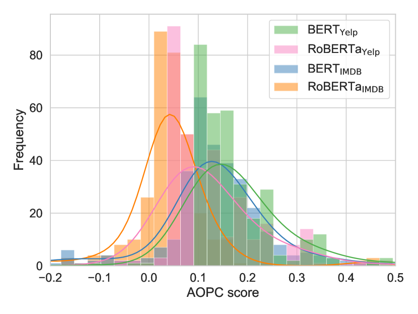
(a) Lower limit

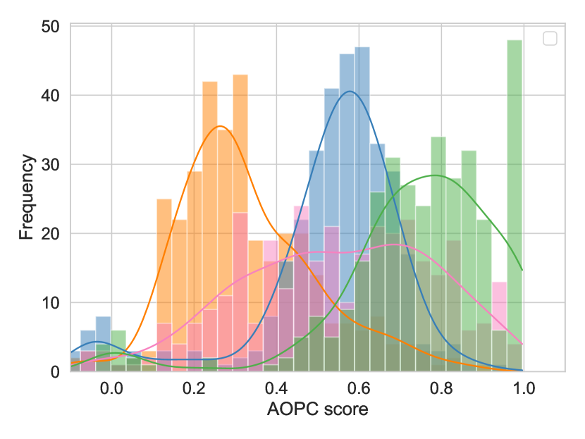
(b) Upper limit

Figure 1: Distributions of lower and upper AOPC limits for different models on the Yelp${}_{\text{short}}$ test set. The figure demonstrates that the lower and upper AOPC limits are model-specific. We excluded models trained on SST-2 for visibility.

Experiment 1: Do the upper and lower limits vary between models?

We aim to show that the lower and upper limits of the AOPC scores vary between the models and inputs. We do so by calculating each model’s upper and lower AOPC limits using an exhaustive search for each example in Yelp${}_{\text{short}}$ (same strategy used by NAOPC${}_{\text{exact}}$). We then compare the models’ lower and upper limit distributions to demonstrate their differences.

Experiment 2: How does normalization impact AOPC scores?

In this experiment, we aim to answer the following two questions:

1. Can NAOPC alter the faithfulness ranking of models for a given feature attribution method?

2. Can NAOPC alter the faithfulness ranking of feature attribution methods for a given model?

To answer these questions, we compare the sufficiency and comprehensiveness scores using AOPC and NAOPC. Specifically, we compare AOPC with NAOPC${}_{\text{beam}}$ for all possible pairs of models and feature attribution methods on the Yelp${}_{\text{long}}$, IMDB${}_{\text{long}}$, and SST2${}_{\text{long}}$ datasets. For the Yelp${}_{\text{short}}$ and SST2${}_{\text{short}}$ datasets, we compare AOPC with both NAOPC${}_{\text{exact}}$ and NAOPC${}_{\text{beam}}$. We analyze the results to find whether NAOPC changes the ranking of which models and feature attribution methods are the most faithful. We use a beam size of 5 when calculating NAOPC${}_{\text{beam}}$.

Experiment 3: Can we approximate NAOPC${}_{\text{exact}}$ reliably and efficiently?

We aim to demonstrate that NAOPC${}_{\text{beam}}$ is a fast and reliable approximation of NAOPC${}_{\text{exact}}$. First, we demonstrate that the faithfulness rankings produced with NAOPC${}_{\text{beam}}$ and NAOPC${}_{\text{exact}}$ are similar on Yelp${}_{\text{short}}$ and SST2${}_{\text{short}}$. We cannot make this comparison on the three other dataset subsets because calculating NAOPC${}_{\text{exact}}$ on high-dimensional inputs is prohibitively slow. Instead, we calculate NAOPC${}_{\text{beam}}$ with increasing beam sizes and analyze the change in results.

Results

The lower and upper limits vary between models

Figure 1 shows significant variations in the distributions of lower and upper AOPC score limits across different models on the Yelp${}_{\text{short}}$ test set. Each model has a distribution rather than a single value because individual inputs also influence the AOPC limits for each model. The clear differences in these distributions across models highlight that direct comparisons of comprehensiveness and sufficiency scores between models can be misleading without proper normalization. Moreover, these variations make interpreting AOPC scores in absolute terms challenging. For instance, an AOPC score of 0.25 might be considered high for RoBERTa${}_{\text{IMDB}}$ but low for BERT${}_{\text{Yelp}}$. These distribution shifts across models emphasize the need for NAOPC. In Appendix B, we provide distributions of lower and upper AOPC score limits across different models on the SST2${}_{\text{short}}$.

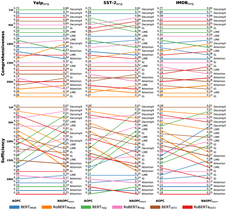
Figure 2: Faithfulness ranking of model and feature attribution method pairs when evaluated using AOPC and NAOPC${}_{\text{beam}}$.This figure shows that normalization changes the cross-model comparisons but not the within-model comparisons.

NAOPC alters faithfulness rankings

Normalization through NAOPC substantially altered models’ faithfulness rankings while preserving the relative performance of feature attribution methods. This effect is clearly visible in Figure 2, where lines of different colors (representing different models) frequently intersect between AOPC and NAOPC${}_{\text{beam}}$ rankings across Yelp${}_{\text{long}}$, IMDB${}_{\text{long}}$, and SST2${}_{\text{long}}$ datasets. In contrast, lines of the same color (representing feature attribution methods within a model) rarely cross, indicating stability in their relative rankings. The impact of normalization appears even more pronounced in shorter text datasets, as shown in Figure 3 for Yelp${}_{\text{short}}$.

These visual observations are quantitatively supported by the Kendall rank correlation coefficients presented in Table 4. For model comparisons, correlations between AOPC and NAOPC${}_{\text{beam}}$ scores are notably lower for sufficiency (ranging from 0.43 to 0.72) than for comprehensiveness (0.87 to 0.93), confirming that normalization significantly impacts model rankings, especially for sufficiency metrics. In contrast, feature attribution methods show consistently high correlations (0.90 to 0.99) for both comprehensiveness and sufficiency across all datasets, underscoring their ranking stability under normalization. This pattern is consistent across all datasets.

Dataset	Group	Comprehensiveness	Sufficiency
Yelp${}_{\text{long}}$	Model	0.87	0.47
	FA	0.97	0.97
SST-2${}_{\text{long}}$	Model	0.89	0.43
	FA	0.90	0.92
IMDB${}_{\text{long}}$	Model	0.93	0.72
	FA	0.99	0.97

Table 4: Kendall rank correlation coefficients between AOPC and NAOPC${}_{\text{beam}}$ rankings across datasets. Coefficients are calculated separately for model rankings and feature attribution method (FA) rankings, showing that normalization impacts the model rankings more than the feature attribution method rankings.

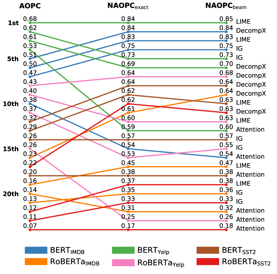
(a) Comprehensiveness ranking

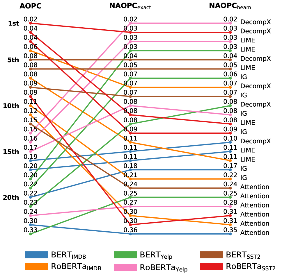
(b) Sufficiency ranking

Figure 3: Faithfulness ranking of model and feature attribution method pairs when evaluated on Yelp${}_{\text{short}}$ using AOPC, NAOPC${}_{\text{exact}}$, and NAOPC${}_{\text{beam}}$. The figure shows that normalization changes the cross-model comparisons and that NAOPC${}_{\text{beam}}$ accurately approximates NAOPC${}_{\text{exact}}$

NAOPC${}_{\text{beam}}$ accurately approximates NAOPC${}_{\text{exact}}$

Our analysis demonstrates that NAOPC${}_{\text{beam}}$ accurately approximates NAOPC${}_{\text{exact}}$ across various dataset dimensions. For low-dimensional input examples, Figure 3 shows nearly identical rankings produced by NAOPC${}_{\text{beam}}$ and NAOPC${}_{\text{exact}}$ on Yelp${}_{\text{short}}$. We provide similar results observed for SST2${}_{\text{short}}$ in Appendix C. For high-dimensional inputs, Figure 4 reveals that increasing the beam size beyond 5 yields minimal changes in the identified lower and upper limits for RoBERTa${}_{\text{Yelp}}$ and BERT${}_{\text{Yelp}}$ on Yelp${}_{\text{long}}$, while we show comparable outcomes for a broad range of models and datasets in Appendix D. Importantly, NAOPC${}_{\text{beam}}$ with a beam size of 5 proves efficient for practical use, requiring an average of  2 minutes per example in Yelp${}_{\text{long}}$ on a single A100 GPU while maintaining accuracy.

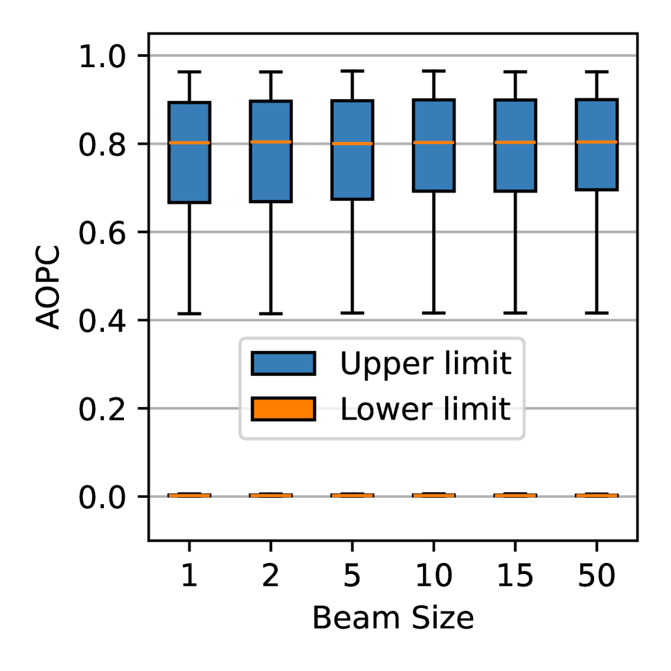
(a) RoBERTa${}_{\text{Yelp}}$

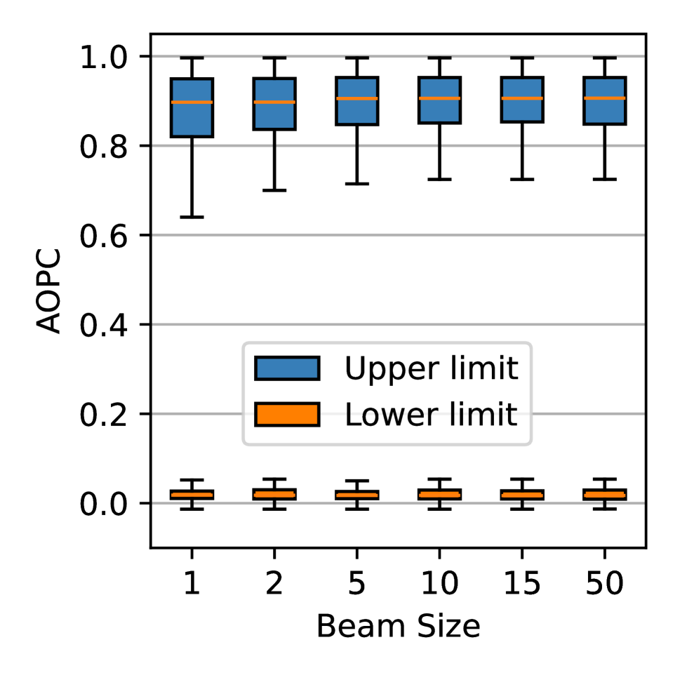
(b) BERT${}_{\text{Yelp}}$

Figure 4: The lower and upper AOPC limits calculated with NAOPC${}_{\text{beam}}$ on Yelp${}_{\text{long}}$ using different beam sizes.

Discussion

Should one always normalize the AOPC scores?

Our findings demonstrate that AOPC scores must be normalized for cross-model comparisons and for meaningful interpretation of individual scores. For cross-model comparisons, normalization is necessary even when comparing models with identical architectures trained on the same dataset but with different seeds. Unnormalized scores can rank feature attribution methods for a single model, but they do not indicate how the scores relate to the model’s possible AOPC score range. Therefore, we recommend normalizing AOPC scores in all cases except when merely ranking attribution methods for a single model. These insights suggest that previous conclusions about model faithfulness may need re-evaluation, considering the importance of score normalization.

Why are some models more faithful than others?

We hypothesize that variations in model faithfulness stem from differences in how closely a model’s reasoning aligns with feature attribution methods’ assumptions. Faithfulness measures how accurately these methods’ assumed reasoning reflects the model’s actual process. Most feature attribution methods use simplified assumptions about model reasoning, such as feature independence (Bilodeau et al. 2024). Consequently, these methods may favor models processing features more independently (like linear models) over those using complex feature interactions. This bias is evident in our results, where models like RoBERTa${}_{\text{IMDB}}$ consistently achieve low comprehensiveness scores across all tested attribution methods, even after normalization.

Limitations

Our findings indicate that normalization did not alter the faithfulness ranking of feature attribution methods within a model. This suggests that normalization is unnecessary when comparing AOPC scores produced using one model and one dataset. Nonetheless, our evaluation did not cover a sufficient variety of models, tasks, and datasets to rule out the necessity of normalization for certain within-model comparisons. We leave the evaluation of more models, datasets, and tasks to future work.

In addition, we demonstrate that increasing NAOPC${}_{\text{beam}}$’s beam size from 5 to 50 had little effect on the results and, therefore, assumed that a beam size of 5 was sufficiently accurate. This assumption could be false. There could be a sudden jump in accuracy if the beam size were increased further. We stopped at beam size 50 because of our computational budget. However, its accuracy in examples with few features supports our claim of accuracy.

Related Work

Researchers have raised several criticisms against AOPC and other perturbation-based faithfulness metrics, which fall into three main categories. First, perturbing inputs can create out-of-distribution examples, potentially conflating distribution shifts with feature importance (Ancona et al. 2017; Hooker et al. 2019; Hase, Xie, and Bansal 2021). Second, perturbations often yield inputs that appear non-sensical to humans, though this should not affect faithfulness evaluation (Feng et al. 2018; Bastings and Filippova 2020; Jacovi and Goldberg 2020). Third, these metrics can be viewed as attribution methods themselves, potentially measuring similarity between methods rather than true faithfulness (Zhou and Shah 2022; Ju et al. 2023).

Alongside AOPC, the field has developed a wide range of faithfulness metrics. These generally fall into two categories: ordering-based and completeness-based. Ordering-based metrics measure whether attributions correctly order input features by importance. These include AOPC, Decision-flip metrics (Chrysostomou and Aletras 2022), Monotonicity and CORR (Arya et al. 2019), and soft-comprehensiveness and soft-sufficiency (Yin et al. 2021; Zhao and Aletras 2023). Completeness-based metrics assess how accurately each feature’s attribution score reflects its impact on the output, with sensitivity-n (Ancona et al. 2017) being the most adopted.

Our work focuses on sufficiency and comprehensiveness due to their widespread use in cross-model comparisons (Bhalla, Srinivas, and Lakkaraju 2023; Li et al. 2023; Chrysostomou and Aletras 2022; Liu et al. 2022).

Conclusion

Our study exposes critical weaknesses in current faithfulness evaluation practices for feature attribution methods. We found that models’ reasoning processes significantly influence AOPC’s lower and upper limits, potentially leading to misleading cross-model comparisons. Moreover, without knowing these limits, it becomes difficult to interpret AOPC scores effectively. These findings challenge the validity of conclusions drawn from cross-model AOPC score comparisons in many influential studies on model faithfulness. To address these issues, we introduced NAOPC, a normalized measure that mitigates model-dependent bias while preserving the ability to compare feature attribution methods within individual models. NAOPC enables more accurate and reliable evaluations of feature attribution methods across different models, advancing the field towards more robust assessments of model faithfulness.

Appendix A Model Details and Access

In table 5, we present an overview of the six models used in our study. For each model, we provide details on the architecture, training data, and a direct link to the corresponding pre-trained weights available on HuggingFace.

Table 5: Overview of the public models from Hugging Face used in this paper.

Model	Architecture	Training data	HuggingFace link
BERT${}_{\text{Yelp}}$	BERT	Yelp	textattack/bert-base-uncased-yelp-polarity
RoBERTa${}_{\text{Yelp}}$	RoBERTa	Yelp	VictorSanh/roberta-base-finetuned-yelp-polarity
BERT${}_{\text{IMDB}}$	BERT	IMBD	textattack/bert-base-uncased-imdb
RoBERTa${}_{\text{IMDB}}$	RoBERTa	IMBD	textattack/roberta-base-imdb
BERT${}_{\text{SST2}}$	BERT	SST2	textattack/bert-base-uncased-SST-2
RoBERTa${}_{\text{SST2}}$	RoBERTa	SST2	textattack/roberta-base-SST-2

Appendix B Analysis of AOPC Score Limit Variability Across Models on the SST2 Dataset

Figure 5 shows the distributions of lower and upper AOPC score limits for different models on the SST2${}_{\text{short}}$ test set. The presence of distributions rather than single values for each model highlights the influence of individual inputs on AOPC limits. The notable differences in these distributions across models underscore the importance of normalization when comparing comprehensiveness and sufficiency scores between models.

(a) Lower AOPC limit

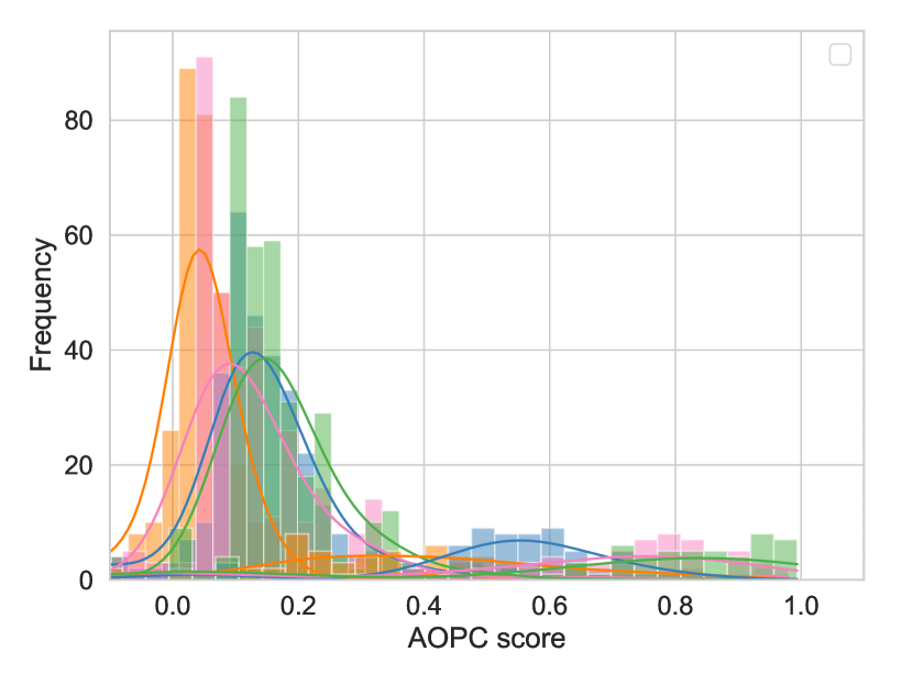
(b) Upper AOPC limit

Figure 5: Distributions of lower and upper AOPC limits for various models on the SST2${}_{\text{short}}$ test set. Each distribution reflects the range of possible AOPC scores for a given model, influenced by individual input examples. The inter-model variations demonstrate the need for normalization when comparing AOPC scores across different models.

Appendix C NAOPC Comparison on SST2${}_{\text{short}}$

This section presents a detailed comparison of NAOPC${}_{\text{beam}}$ and NAOPC${}_{\text{exact}}$ on the SST2${}_{\text{short}}$ dataset. Figure 6 illustrates the rankings produced by both methods when evaluating the comprehensiveness and sufficiency of the dataset. The figure shows almost identical rankings produced by NAOPC${}_{\text{beam}}$ and NAOPC${}_{\text{exact}}$.

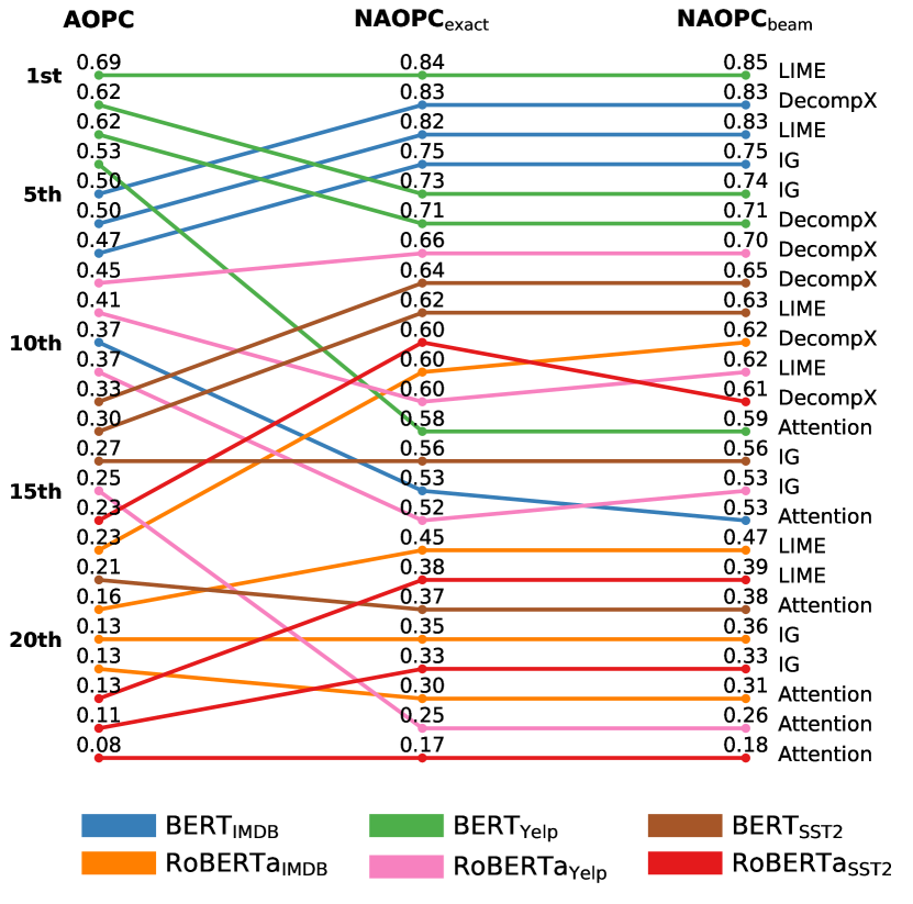
(a) Comprehensiveness Order

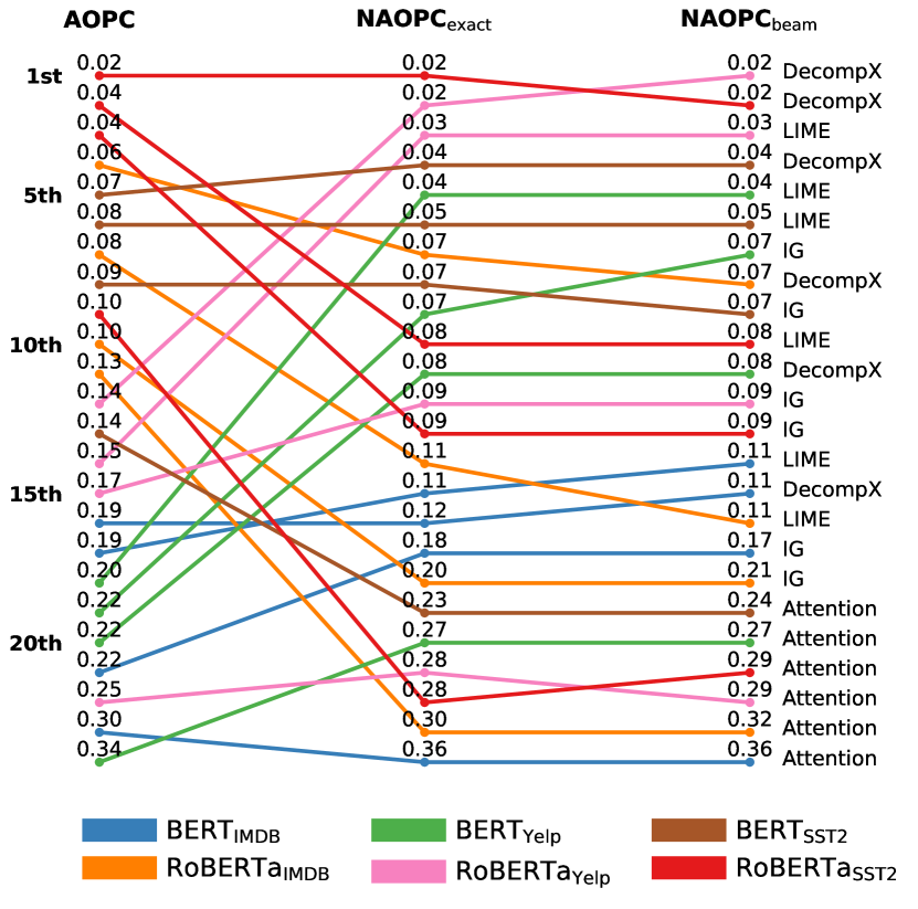
(b) Sufficiency Order

Figure 6: The difference in rankings when normalizing on the SST-2 dataset

Appendix D Impact of Beam Size on NAOPC${}_{\text{beam}}$ Across Various Datasets

As illustrated in fig. 7, the relationship between increasing beam size and NAOPC${}_{\text{beam}}$ is examined across various models and datasets. The findings indicate that while an initial expansion of beam size results in variability in the upper and lower bounds, further increases beyond a beam size of 5 lead to a convergence trend. This pattern is consistently observed across different models and datasets, particularly evident in the results for RoBERTa${}_{\text{Yelp}}$ and BERT${}_{\text{Yelp}}$ on the Yelp${}_{\text{long}}$ dataset.

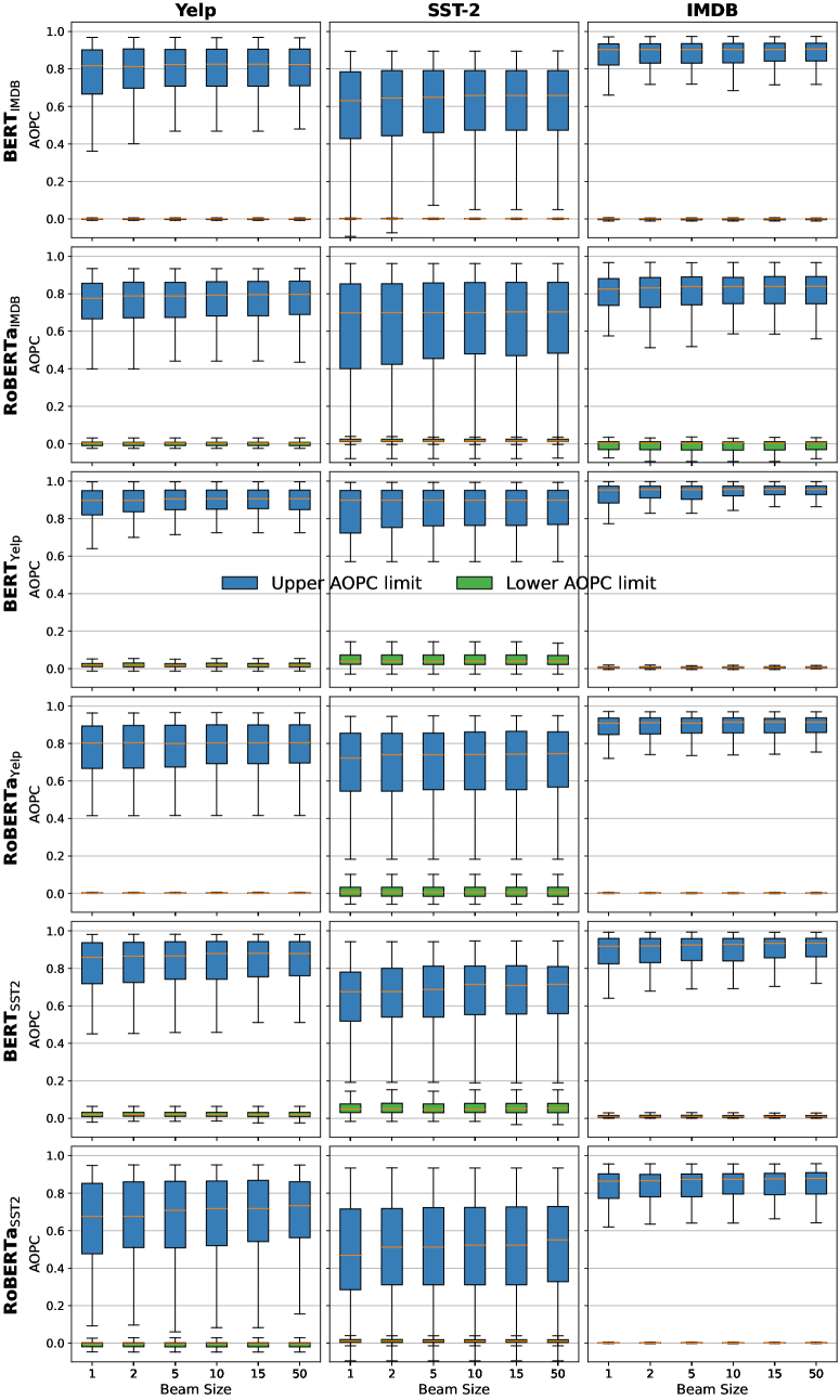
Figure 7: Boxplots showing the distribution of NAOPC${}_{\text{beam}}$ values across different beam sizes for various models and datasets.

.

References

- Ancona et al. (2017) Ancona, M.; Ceolini, E.; Öztireli, C.; and Gross, M. 2017. Towards better understanding of gradient-based attribution methods for deep neural networks. arXiv preprint arXiv:1711.06104.
- Arya et al. (2019) Arya, V.; Bellamy, R. K.; Chen, P.-Y.; Dhurandhar, A.; Hind, M.; Hoffman, S. C.; Houde, S.; Liao, Q. V.; Luss, R.; Mojsilović, A.; et al. 2019. One explanation does not fit all: A toolkit and taxonomy of ai explainability techniques. arXiv preprint arXiv:1909.03012.
- Bastings and Filippova (2020) Bastings, J.; and Filippova, K. 2020. The elephant in the interpretability room: Why use attention as explanation when we have saliency methods? In Alishahi, A.; Belinkov, Y.; Chrupa\la, G.; Hupkes, D.; Pinter, Y.; and Sajjad, H., eds., Proceedings of the Third BlackboxNLP Workshop on Analyzing and Interpreting Neural Networks for NLP, 149–155. Online: Association for Computational Linguistics.
- Bhalla, Srinivas, and Lakkaraju (2023) Bhalla, U.; Srinivas, S.; and Lakkaraju, H. 2023. Discriminative Feature Attributions: Bridging Post Hoc Explainability and Inherent Interpretability. In Advances in Neural Information Processing Systems 36 (NeurIPS 2023).
- Bhatt, Weller, and Moura (2020) Bhatt, U.; Weller, A.; and Moura, J. M. F. 2020. Evaluating and Aggregating Feature-based Model Explanations. ArXiv:2005.00631 [cs, stat].
- Bilodeau et al. (2024) Bilodeau, B.; Jaques, N.; Koh, P. W.; and Kim, B. 2024. Impossibility theorems for feature attribution. Proceedings of the National Academy of Sciences, 121(2): e2304406120.
- Chen and Ji (2020) Chen, H.; and Ji, Y. 2020. Learning Variational Word Masks to Improve the Interpretability of Neural Text Classifiers. ArXiv:2010.00667 [cs].
- Chrysostomou and Aletras (2021) Chrysostomou, G.; and Aletras, N. 2021. Enjoy the Salience: Towards Better Transformer-based Faithful Explanations with Word Salience. In Moens, M.-F.; Huang, X.; Specia, L.; and Yih, S. W.-t., eds., Proceedings of the 2021 Conference on Empirical Methods in Natural Language Processing, 8189–8200. Online and Punta Cana, Dominican Republic: Association for Computational Linguistics.
- Chrysostomou and Aletras (2022) Chrysostomou, G.; and Aletras, N. 2022. An Empirical Study on Explanations in Out-of-Domain Settings. In Proceedings of the 60th Annual Meeting of the Association for Computational Linguistics (Volume 1: Long Papers), 6920–6938. Dublin, Ireland: Association for Computational Linguistics.
- Danilevsky et al. (2020) Danilevsky, M.; Qian, K.; Aharonov, R.; Katsis, Y.; Kawas, B.; and Sen, P. 2020. A Survey of the State of Explainable AI for Natural Language Processing. In Proceedings of the 1st Conference of the Asia-Pacific Chapter of the Association for Computational Linguistics and the 10th International Joint Conference on Natural Language Processing, 447–459. Suzhou, China: Association for Computational Linguistics.
- Devlin et al. (2019) Devlin, J.; Chang, M.-W.; Lee, K.; and Toutanova, K. 2019. BERT: Pre-training of Deep Bidirectional Transformers for Language Understanding. arXiv:1810.04805 [cs]. 9999 citations (Semantic Scholar/arXiv) [2023-01-05] arXiv: 1810.04805.
- DeYoung et al. (2020) DeYoung, J.; Jain, S.; Rajani, N. F.; Lehman, E.; Xiong, C.; Socher, R.; and Wallace, B. C. 2020. ERASER: A Benchmark to Evaluate Rationalized NLP Models. In Proceedings of the 58th Annual Meeting of the Association for Computational Linguistics, 4443–4458. Online: Association for Computational Linguistics.
- Feng et al. (2018) Feng, S.; Wallace, E.; Grissom II, A.; Iyyer, M.; Rodriguez, P.; and Boyd-Graber, J. 2018. Pathologies of neural models make interpretations difficult. arXiv preprint arXiv:1804.07781.
- Hase, Xie, and Bansal (2021) Hase, P.; Xie, H.; and Bansal, M. 2021. The Out-of-Distribution Problem in Explainability and Search Methods for Feature Importance Explanations. In 35th Conference on Neural Information Processing Systems (NeurIPS 2021). arXiv. ArXiv:2106.00786 [cs].
- Hooker et al. (2019) Hooker, S.; Erhan, D.; Kindermans, P.-J.; and Kim, B. 2019. A Benchmark for Interpretability Methods in Deep Neural Networks. In Advances in Neural Information Processing Systems, volume 32. Curran Associates, Inc.
- Jacovi and Goldberg (2020) Jacovi, A.; and Goldberg, Y. 2020. Towards Faithfully Interpretable NLP Systems: How Should We Define and Evaluate Faithfulness? In Proceedings of the 58th Annual Meeting of the Association for Computational Linguistics, 4198–4205. Online: Association for Computational Linguistics.
- Jain and Wallace (2019) Jain, S.; and Wallace, B. C. 2019. Attention is not Explanation. ArXiv:1902.10186 [cs].
- Ju et al. (2023) Ju, Y.; Zhang, Y.; Yang, Z.; Jiang, Z.; Liu, K.; and Zhao, J. 2023. Logic Traps in Evaluating Attribution Scores. ArXiv:2109.05463 [cs].
- Li et al. (2023) Li, D.; Hu, B.; Chen, Q.; and He, S. 2023. Towards Faithful Explanations for Text Classification with Robustness Improvement and Explanation Guided Training. In Ovalle, A.; Chang, K.-W.; Mehrabi, N.; Pruksachatkun, Y.; Galystan, A.; Dhamala, J.; Verma, A.; Cao, T.; Kumar, A.; and Gupta, R., eds., Proceedings of the 3rd Workshop on Trustworthy Natural Language Processing (TrustNLP 2023), 1–14. Toronto, Canada: Association for Computational Linguistics.
- Lipton (2018) Lipton, Z. C. 2018. The mythos of model interpretability: In machine learning, the concept of interpretability is both important and slippery. Queue, 16(3): 31–57.
- Liu et al. (2022) Liu, J.; Lin, Y.; Jiang, L.; Liu, J.; Wen, Z.; and Peng, X. 2022. Improve Interpretability of Neural Networks via Sparse Contrastive Coding. In Goldberg, Y.; Kozareva, Z.; and Zhang, Y., eds., Findings of the Association for Computational Linguistics: EMNLP 2022, 460–470. Abu Dhabi, United Arab Emirates: Association for Computational Linguistics.
- Liu et al. (2019) Liu, Y.; Ott, M.; Goyal, N.; Du, J.; Joshi, M.; Chen, D.; Levy, O.; Lewis, M.; Zettlemoyer, L.; and Stoyanov, V. 2019. RoBERTa: A Robustly Optimized BERT Pretraining Approach. arXiv:1907.11692 [cs]. 9993 citations (Semantic Scholar/arXiv) [2023-01-05] arXiv: 1907.11692.
- Lundberg and Lee (2017) Lundberg, S. M.; and Lee, S.-I. 2017. A Unified Approach to Interpreting Model Predictions. In Advances in Neural Information Processing Systems, volume 30. Curran Associates, Inc.
- Lyu, Apidianaki, and Callison-Burch (2024) Lyu, Q.; Apidianaki, M.; and Callison-Burch, C. 2024. Towards Faithful Model Explanation in NLP: A Survey. arXiv:2209.11326.
- Maas et al. (2011) Maas, A. L.; Daly, R. E.; Pham, P. T.; Huang, D.; Ng, A. Y.; and Potts, C. 2011. Learning Word Vectors for Sentiment Analysis. In Lin, D.; Matsumoto, Y.; and Mihalcea, R., eds., Proceedings of the 49th Annual Meeting of the Association for Computational Linguistics: Human Language Technologies, 142–150. Portland, Oregon, USA: Association for Computational Linguistics.
- Modarressi et al. (2023) Modarressi, A.; Fayyaz, M.; Aghazadeh, E.; Yaghoobzadeh, Y.; and Pilehvar, M. T. 2023. DecompX: Explaining Transformers Decisions by Propagating Token Decomposition. In Rogers, A.; Boyd-Graber, J.; and Okazaki, N., eds., Proceedings of the 61st Annual Meeting of the Association for Computational Linguistics (Volume 1: Long Papers), 2649–2664. Toronto, Canada: Association for Computational Linguistics.
- Morris et al. (2020) Morris, J. X.; Lifland, E.; Yoo, J. Y.; Grigsby, J.; Jin, D.; and Qi, Y. 2020. TextAttack: A Framework for Adversarial Attacks, Data Augmentation, and Adversarial Training in NLP. ArXiv:2005.05909 [cs].
- Nielsen et al. (2023) Nielsen, I. E.; Ramachandran, R. P.; Bouaynaya, N.; Fathallah-Shaykh, H. M.; and Rasool, G. 2023. EvalAttAI: A Holistic Approach to Evaluating Attribution Maps in Robust and Non-Robust Models. IEEE Access, 11: 82556–82569. Conference Name: IEEE Access.
- Resck, Raimundo, and Poco (2024) Resck, L. E.; Raimundo, M. M.; and Poco, J. 2024. Exploring the Trade-off Between Model Performance and Explanation Plausibility of Text Classifiers Using Human Rationales. ArXiv:2404.03098 [cs].
- Ribeiro, Singh, and Guestrin (2016) Ribeiro, M. T.; Singh, S.; and Guestrin, C. 2016. ”Why Should I Trust You?”: Explaining the Predictions of Any Classifier. In Proceedings of the 22nd ACM SIGKDD International Conference on Knowledge Discovery and Data Mining, 1135–1144. San Francisco California USA: ACM. ISBN 978-1-4503-4232-2.
- Samek et al. (2016) Samek, W.; Binder, A.; Montavon, G.; Lapuschkin, S.; and Müller, K.-R. 2016. Evaluating the visualization of what a deep neural network has learned. IEEE transactions on neural networks and learning systems, 28(11): 2660–2673.
- Sekhon et al. (2023) Sekhon, A.; Chen, H.; Shrivastava, A.; Wang, Z.; Ji, Y.; and Qi, Y. 2023. Improving Interpretability via Explicit Word Interaction Graph Layer. Proceedings of the AAAI Conference on Artificial Intelligence, 37(11): 13528–13537. Number: 11.
- Shrikumar, Greenside, and Kundaje (2017) Shrikumar, A.; Greenside, P.; and Kundaje, A. 2017. Learning important features through propagating activation differences. In Proceedings of the 34th International Conference on Machine Learning - Volume 70, ICML’17, 3145–3153. Sydney, NSW, Australia: JMLR.org.
- Socher et al. (2013) Socher, R.; Perelygin, A.; Wu, J.; Chuang, J.; Manning, C. D.; Ng, A.; and Potts, C. 2013. Recursive Deep Models for Semantic Compositionality Over a Sentiment Treebank. In Yarowsky, D.; Baldwin, T.; Korhonen, A.; Livescu, K.; and Bethard, S., eds., Proceedings of the 2013 Conference on Empirical Methods in Natural Language Processing, 1631–1642. Seattle, Washington, USA: Association for Computational Linguistics.
- Sundararajan, Taly, and Yan (2017) Sundararajan, M.; Taly, A.; and Yan, Q. 2017. Axiomatic Attribution for Deep Networks. In Proceedings of the 34th International Conference on Machine Learning, 3319–3328. PMLR. ISSN: 2640-3498.
- Tsang, Rambhatla, and Liu (2020) Tsang, M.; Rambhatla, S.; and Liu, Y. 2020. How does This Interaction Affect Me? Interpretable Attribution for Feature Interactions. In Advances in Neural Information Processing Systems, volume 33, 6147–6159. Curran Associates, Inc.
- Wei et al. (2022) Wei, J.; Tay, Y.; Bommasani, R.; Raffel, C.; Zoph, B.; Borgeaud, S.; Yogatama, D.; Bosma, M.; Zhou, D.; Metzler, D.; Chi, E. H.; Hashimoto, T.; Vinyals, O.; Liang, P.; Dean, J.; and Fedus, W. 2022. Emergent Abilities of Large Language Models. arXiv:2206.07682.
- Yin et al. (2021) Yin, F.; Shi, Z.; Hsieh, C.-J.; and Chang, K.-W. 2021. On the sensitivity and stability of model interpretations in NLP. arXiv preprint arXiv:2104.08782.
- Zhang, Zhao, and LeCun (2015) Zhang, X.; Zhao, J.; and LeCun, Y. 2015. Character-level Convolutional Networks for Text Classification. In Advances in Neural Information Processing Systems, volume 28. Curran Associates, Inc.
- Zhao and Aletras (2023) Zhao, Z.; and Aletras, N. 2023. Incorporating attribution importance for improving faithfulness metrics. arXiv preprint arXiv:2305.10496.
- Zhou and Shah (2022) Zhou, Y.; and Shah, J. 2022. The solvability of interpretability evaluation metrics. arXiv preprint arXiv:2205.08696.