Combined p-value functions for meta-analysis

Highlights

What is already known

• $P$-value functions are statistical tools that unify frequentist hypothesis testing and parameter estimation, and are therefore particularly useful for quantitative reporting of statistical analyses. • Meta-analysis based on p-value combination methods can be unified with model-based meta-analysis using $p$-value functions.

What is new

• $P$-value functions of different p-value combination methods for meta-analysis are compared theoretically and with a simulation study, heterogeneity adjustments are proposed. • $P$-value function methods for meta-analysis are implemented in the R package confMeta.

Potential impact

• Edgington’s combination method based on the sum of p-values is recommended as an alternative to standard fixed effect or random effects meta-analysis because of its ability to reflect data asymmetry, its orientation-invariance, and its good operating characteristics.

1 Introduction

A pervasive challenge in all areas of research is the assessment of evidence from multiple studies. Standard meta-analysis aims to synthesize effect estimates from several studies into an overall effect estimate, typically a weighted average of the study-specific effect estimates, combined with an appropriate confidence interval. Inverse-variance weights can be motivated as efficient choices under homogeneity or heterogeneity between studies (Rice et al., , 2018) via either exchangeability or random sampling of study effects (Higgins et al., , 2009). Random effects meta-analysis incorporates a measure of heterogeneity into the weights. This form of weights gives an estimate that is consistent for the mean of the distribution of study effects, a natural target of inference where a symmetric (usually normal) distribution can be assumed.

There has been much progress in proposing alternative confidence intervals for meta-analysis. The approach by Hartung and Knapp, (2001) and Sidik and Jonkman, (2002) takes into account the uncertainty in estimating heterogeneity and tends to produce wider confidence intervals. The approach by Henmi and Copas, (2010) combines the fixed effect point estimate with a standard error from the random effects model, in order to obtain confidence intervals less prone to publication bias. However, all these intervals are of a simple additive form with limits

$$\mbox{ point estimate }\pm\mbox{ additive factor, }$$ (1)

so symmetric around the point estimate. This may be reasonable if there is good reason to assume that the true effect estimates follow a symmetric (normal) distribution around their mean, but confidence intervals not restricted to be symmetric around the point estimate may be more suitable if this assumption cannot be made.

There is not much literature on meta-analysis of skewed data. Higgins et al., (2008) focus on possible transformations of skewed outcome data, where results are reported on a log-transformed scale for some studies, but on the raw scale for other studies. Yang et al., (2016) consider $p$-value combination methods for rare events based on Fisher’s exact test and note in an application to simulated data that “the $p$-value function based on the exact test preserves the skewness” of the original data. This statement suggests that a desired property of meta-analytic confidence interval is to reflect data asymmetry. However, the authors did not investigate this feature any further.

In this paper we will compare meta-analytic methods based on the combined $p$-value function (Fraser, , 2019; Infanger and Schmidt-Trucksäss, , 2019) or equivalently confidence curve (Bender et al., , 2005) and confidence distribution (Marschner, , 2024; Melilli and Veronese, , 2024). Related meta-analytic approaches based on $p$-value functions have been proposed by Singh et al., (2005). They showed that $p$-value combination based meta-analysis – approaches that combine $p$-values of individual studies, such as Fisher’s method – can be unified with model-based meta-analysis under a common framework using $p$-value functions. This framework has subsequently been extended (Xie et al., , 2011; Liu et al., , 2014; Yang et al., , 2016; Zabriskie et al., , 2021), but has not yet gained much traction in the applied meta-analysis literature. Another proposal related to the $p$-value function is the “drapery plot” of Rücker and Schwarzer, (2020). This visualization shows the $p$-value functions of individual studies and of their pooled effect, providing the reader with a wealth of information as $p$-values and confidence intervals (at any level) can be easily read off.

We apply the same ideas in our article and provide a systematic comparison of different types of $p$-value combination procedures (Hedges and Olkin, , 1985; Cousins, , 2007). Theory and simulation studies are used to compare the different confidence intervals and point estimates in terms of coverage, width, bias, and skewness. We eventually recommend Edgington’s method (Edgington, 1972a, ; Edgington, 1972b, ) based on the sum of $p$-values as an alternative to standard fixed effect or random effects meta-analysis.

2 Methodology

Let $\hat{\theta}_{i}$ denote the effect estimate of the true parameter $\theta_{i}$ from the $i$-th study, $i=1,\ldots,n$, and $\sigma_{i}$ the corresponding standard error. As in standard meta-analysis we assume that the $\hat{\theta}_{i}$’s are independent and follow a normal distribution with unknown mean $\theta_{i}$ and known variance $\sigma_{i}^{2}$ (the squared standard error). Additional adjustments for heterogeneity will be discussed in Section 2.3.

Let

$$Z_{i}=\frac{\hat{\theta}_{i}-\mu}{\sigma_{i}}$$ (2)

denote the $z$-statistic for the null hypothesis $H_{0i}$: $\theta_{i}=\mu$, $i=1,\ldots,n$. We can then derive the corresponding one-sided $p$-values

$$\overset{\rightharpoonup}{p_{i}}=1-\Phi(Z_{i})\mbox{ and }\overset{\leftharpoonup}{p_{i}}=\Phi(Z_{i})$$ (3)

for the alternatives $H_{1i}$: $\theta_{i}>\mu$ ("greater") and $H_{1i}$: $\theta_{i}<\mu$ ("less"), respectively. Note that $\overset{\rightharpoonup}{p_{i}}$ is monotonically increasing and $\overset{\leftharpoonup}{p_{i}}$ is monotonically decreasing in $\mu$.

2.1 P-value combination methods

In what follows we denote with $\overset{\rightharpoonup}{p_{\bullet}}$ a combined $p$-value based on study-specific one-sided $p$-values $\overset{\rightharpoonup}{p_{1}},\ldots,\overset{\rightharpoonup}{p_{n}}$ for the alternative "greater" and likewise with $\overset{\leftharpoonup}{p_{\bullet}}$ for the alternative "less". The subscript $\bullet$ is a placeholder for a $p$-value combination method, abbreviated by the first letter of the last name of the inventor, where we consider the methods listed in Table 1:

• Edgington’s method (Edgington, 1972a, ),

• Fisher’s method (Fisher, , 1932),

• Pearson’s method (Pearson, , 1933),

• Wilkinson’s method (Wilkinson, , 1951), and

• Tippett’s method (Tippett, , 1931).

The combined $p$-values $\overset{\rightharpoonup}{p_{\bullet}}$ and $\overset{\leftharpoonup}{p_{\bullet}}$ will inherit the monotonicity property from the $\overset{\rightharpoonup}{p_{i}}$’s and $\overset{\leftharpoonup}{p_{i}}$’s, respectively: $\overset{\rightharpoonup}{p_{\bullet}}$ is monotonically increasing and $\overset{\leftharpoonup}{p_{\bullet}}$ is monotonically decreasing in $\mu$ for any of the combination methods listed in Table 1.

Table 1: Some methods for combining one-sided $p$-values ${p_{1}},\dots,{p_{n}}$ from $n$ studies into a combined $p$-value ${p_{\bullet}}$ (in alphabetic order). A chi-squared random variable with $n$ degrees of freedom is denoted as $\chi^{2}_{n}$.

Method	Combined p-value
Edgington	${p_{E}}=\frac{1}{n!}\sum_{k=0}^{\lfloor{s}\rfloor}(-1)^{k}\binom{n}{k}({s}-k)^{n}$ with ${s}=\sum_{i=1}^{n}{p_{i}}$
Fisher	${p_{F}}=\Pr(\chi^{2}_{2n}>{f})$ with ${f}=-2\sum_{i=1}^{n}\log({p_{i}})$
Pearson	${p_{P}}=\Pr(\chi^{2}_{2n}\leq{k})$ with ${k}=-2\sum_{i=1}^{n}\log(1-{p_{i}})$
Tippett	${p_{T}}=1-(1-\min\{{p}_{1},\dots,{p}_{n}\})^{n}$
Wilkinson	${p_{W}}=\max\{{p}_{1},\dots,{p}_{n}\}^{n}$

The $p$-value from Edgington’s method is based on a transformation of the sum of the $p$-values ${s}$ with the cumulative distribution function of the Irwin-Hall distribution (Irwin, , 1927; Hall, , 1927). For large $n$ it can be approximated based on a central limit theorem argument (Edgington, 1972b, ):

$${p_{E}}\approx\Phi(\sqrt{12\,n}({s}/n-1/2)).$$

In order to mitigate overflow problems of the Irwin-Hall distribution for large $n$, we use this normal approximation if $n>11$.

Tippett’s method is based on the smallest $p$-value. There is a generalization of Tippett’s method based on the $r$-th smallest $p$-value (Wilkinson, , 1951; Hedges and Olkin, , 1985). For $r=n$ the largest $p$-value is hence used and we obtain the method denoted here as Wilkinson’s method. Another commonly used $p$-value combination method is Stouffer’s method based on the sum of inverse normal transformed $p$-values (Stouffer et al., , 1949). A weighted version exists (Cousins, , 2007), which is equivalent to fixed and random effects meta-analysis, if the weights are suitably chosen (Senn, , 2021). Random effects meta-analysis will be included in our simulation study described in Section 3.

Suppose we combine one-sided $p$-values $\overset{\rightharpoonup}{p_{1}},\ldots,\overset{\rightharpoonup}{p_{n}}$ for the alternative "greater" into a combined $p$-value function $\overset{\rightharpoonup}{p_{\bullet}}(\mu)$. The standard point estimate is the median estimate $\hat{\mu}$ (Fraser, , 2017), defined as the root of the equation

$$\overset{\rightharpoonup}{p_{\bullet}}(\hat{\mu})=0.5.$$ (4)

For Edgington’s method the median estimate $\hat{\mu}$ is the value of $\mu$ where the mean of the study-specific one-sided $p$-values is 0.5.

In order to obtain a two-sided $1-\alpha$ confidence interval $[\mu_{l},\mu_{u}]$ for $\mu$ based on a $p$-value combination method $\overset{\rightharpoonup}{p_{\bullet}}$, we have to find the roots $\mu_{l}$ and $\mu_{u}$ of the two equations

$$\overset{\rightharpoonup}{p_{\bullet}}(\mu_{l})=\alpha/2 \overset{\rightharpoonup}{p_{\bullet}}(\mu_{u})=1-\alpha/2.$$ and (5)

The roots in (4) and (5) can be calculated with numerical root-finding algorithms. Equivalently we can find the two roots $\mu_{l}$ and $\mu_{u}$ of the single equation

$$2\,\min\left\{\overset{\rightharpoonup}{p_{\bullet}}(\mu),1-\overset{\rightharpoonup}{p_{\bullet}}(\mu)\right\}=\alpha$$ (6)

to obtain the $1-\alpha$ confidence interval, while maximization of the function on the left side of (6) gives the median estimate $\hat{\mu}$. Note that the confidence intervals $[\mu_{l},\mu_{u}]$ is not necessarily symmetric around the median estimate.

We may also use $\overset{\leftharpoonup}{p_{\bullet}}(\mu)$ (based on the one-sided $p$-values $\overset{\leftharpoonup}{p_{1}},\dots,\overset{\leftharpoonup}{p_{n}}$) rather than $\overset{\rightharpoonup}{p_{\bullet}}(\mu)$ to compute a point estimate with two-sided confidence interval. Ideally this should lead to the same results, but this is only the case for Edgington’s method. The other combination methods will generally lead to different results depending on whether the input $p$-values are oriented "greater" or "less" due to the following relationships between combined $p$-value and input $p$-value orientation:

$$\overset{\rightharpoonup}{p_{E}} = 1-\overset{\leftharpoonup}{p_{E}},$$ (7)

$$\overset{\rightharpoonup}{p_{F}} = 1-\overset{\leftharpoonup}{p_{P}},$$ (8)

$$\overset{\rightharpoonup}{p_{P}} = 1-\overset{\leftharpoonup}{p_{F}},$$ (9)

$$\overset{\rightharpoonup}{p_{T}} = 1-\overset{\leftharpoonup}{p_{W}},$$ (10)

$$\overset{\rightharpoonup}{p_{W}} = 1-\overset{\leftharpoonup}{p_{T}},$$ (11)

see Appendix A for a proof. For example, the combined $p$-value function based on Fisher’s method and one-sided $p$-values for the alternative "greater" is 1 minus the combined $p$-value function based on Pearson’s method and one-sided $p$-values for the alternative "less". However, in practice the ultimate goal is to compute a point estimate with two-sided confidence interval, so the direction of the alternative of the underlying one-sided $p$-values shouldn’t matter. But this is only the case for Edgington’s method.

In principle, we may also use two-sided $p$-values in any of the combination methods listed in Table 1, to circumvent the lack of orientation-invariance of Tippett’s, Wilkinson’s, Fisher’s and Pearson’s method, but this comes with new problems. Specifically, the combined $p$-value function of Fisher’s, Pearson’s and Edgington’s method based on two-sided $p$-values will then no longer peak at 1, which means that confidence intervals on certain confidence levels will be empty sets. In contrast, the combined $p$-value functions of Tippett’s and Wilkinson’s method will peak at one, but will have several modes at the study-specific point estimates. This may lead to confidence sets consisting of non-overlapping intervals, which are hard to interpret and not useful for application in practice.

In summary, we therefore recommend to use Edgington’s method based on one-sided $p$-values, as this is the only method (different from standard meta-analysis) that is orientation-invariant with a unique point estimate and always existing confidence interval. A confidence interval based on Edgington’s method is not necessarily symmetric around the point estimate, so less restrictive than standard meta-analytic confidence intervals of the form (1).

2.2 Example: Association between corticosteroids and mortality in COVID-19 hospitalized patients

We will illustrate the different methods using a meta-analysis combining information from $n=7$ randomized controlled clinical trials investigating the association between corticosteroids and mortality in hospitalized patients with COVID-19 (WHO REACT Working Group, , 2020). The results from a fixed effect analysis are reproduced in Figure 1 on the log odds ratio scale. This was also the primary analysis as specified in the study protocol and the data do not indicate conflict with the fixed effect assumptions based on Cochran’s $Q$-test ($p=0.31$, Higgins’ $I^{2}=16\%$). Figure 1 also shows that the distribution of the study effect estimates is right-skewed. Such skewness can be quantified using Fisher’s weighted skewness coefficient of the meta-analyzed effect estimates, defined as

$$\gamma=\frac{\left\{\sum_{i=1}^{k}(\hat{\theta}_{i}w_{i}-\bar{\theta})^{3}\right\}\sqrt{\sum_{i=1}^{k}w_{i}}}{\left\{\sum_{i=1}^{k}(\hat{\theta}_{i}w_{i}-\bar{\theta})^{2}\right\}^{3/2}}\leavevmode\nobreak\ \text{ with }\leavevmode\nobreak\ \bar{\theta}=\frac{\sum_{i=1}^{k}\hat{\theta}_{i}w_{i}}{\sum_{i=1}^{k}w_{i}}\leavevmode\nobreak\ \text{ and }\leavevmode\nobreak\ w_{i}=\frac{1}{\sigma^{2}_{i}}.$$ (12)

In this example we obtain $\gamma=3.72$, the positive sign reflecting a right-skewed distribution.

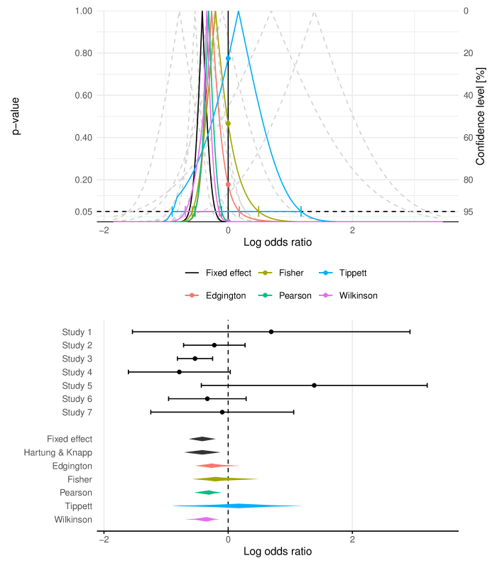
Figure 1: $P$-value function (top) and forest plot (bottom) from several combination methods with 95% confidence intervals for a meta-analysis of $n=7$ randomized controlled clinical trials investigating the association between corticosteroids and mortality in hospitalized patients with COVID-19 (WHO REACT Working Group, , 2020).

Table 2: Comparison of different $p$-value combination methods (with alternative "greater") and their 95% CIs with the fixed effect and Hartung-Knapp approach for meta-analysis of $n=7$ randomized controlled clinical trials investigating the association between corticosteroids and mortality in hospitalized patients with COVID-19. The $p$-value ${p}_{\bullet}(0)$ shown is two-sided for the standard null hypothesis $\mu=0$ of no effect.

	Estimate	Lower CI	Upper CI	${p}_{\bullet}(0)$	CI width	CI skewness
Fixed effect	-0.42	-0.63	-0.20	0.0001	0.43	0.00
Hartung-Knapp	-0.42	-0.71	-0.13	0.013	0.58	0.00
Edgington	-0.27	-0.53	0.18	0.18	0.71	0.26
Fisher	-0.20	-0.58	0.49	0.47	1.07	0.30
Pearson	-0.31	-0.54	-0.10	0.003	0.43	-0.03
Tippett	0.17	-0.90	1.17	0.77	2.08	-0.03
Wilkinson	-0.34	-0.69	-0.15	0.002	0.55	-0.27

We will use one-sided $p$-values for the alternative "greater", the results for the alternative "less" follow from (7)-(11). Results based on the different methods are shown in Table 2. The point estimates from the different $p$-value combination methods are all closer to zero than the combined effect estimate from the fixed effect and Hartung-Knapp method, respectively. Also the 95% confidence intervals differ quite a lot. Tippett’s method even gives a positive point estimate and has the largest interval width. There is also surprisingly large variation of the (two-sided) $p$-value ${p}_{\bullet}(0)$ for the null hypothesis of no effect. To assess the skewness of the different confidence intervals, we computed the skewness coefficient

$$\beta=\frac{\mbox{upper}+\mbox{lower}-2\,\mbox{estimate}}{\mbox{upper}-\mbox{lower}}.$$ (13)

by Groeneveld and Meeden, (1984). Note that $\left\lvert\beta\right\rvert\leq 1$ with positive sign for a right-skewed interval and negative sign for a left-skewed one. The coefficient is zero for symmetric confidence intervals, here for the fixed effect and Hartung-Knapp method. The last column in Table 2 reveals that three of the different $p$-value combination methods (Pearson, Tippett, Wilkinson) return a left-skewed confidence interval with negative skewness coefficient $\beta$, although the study effect estimates are right-skewed. Only Edgington’s and Fisher’s method preserve the skewness of the data and return a positive coefficient $\beta$.

Two of the studies have large confidence intervals due to a small number of events, where the normality assumption in (3) may be questionable. We can also define $p$-value functions based on exact one-sided $p$-values from Fisher’s exact test, where we employ the mid-$p$ correction, originally proposed by Lancaster, (1961). This ensures that the $p$-values for "greater" and "less" still sum up to 1, although the distribution of the test statistic is discrete. Edgington’s method will hence still be orientation-invariant, whereas the other method will not.

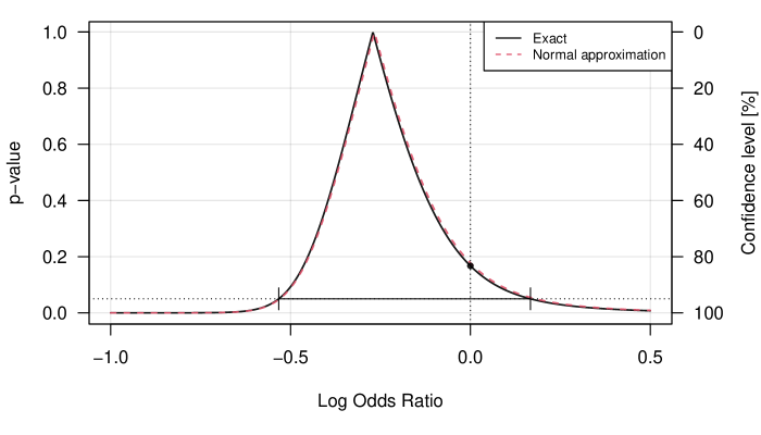
Figure 2: Edgington’s combined $p$-value function with 95% confidence interval based on exact $p$-values with mid-$p$ correction for meta-analysis of $n=7$ randomized controlled clinical trials investigating the association between corticosteroids and mortality in hospitalized patients with COVID-19 (WHO REACT Working Group, , 2020). Shown is also the normal approximation $p$-value function based on the $z$-statistics (2) for comparison.

Figure 2 shows the corresponding $p$-value function and confidence density based on the exact $p$-values (solid black line) along with the normal approximation $p$-value function based on the $z$-statistics (2) as comparison (dashed red line). We see that both curves are virtually identical, producing almost identical point estimates, $p$-values, and confidence intervals. This suggests that the $p$-value function based on the $z$-statistics provides a good approximation to the one based exact $p$-values, despite small counts for some of the studies.

2.3 Accounting for heterogeneity

The $z$-statistic (2) can be modified to account for heterogeneity between studies. Here we consider the case of additive heterogeneity, where heterogeneity is estimated based on Cochran’s $Q$-statistic (Cochran, , 1937)

$$Q=\sum\limits_{i=1}^{k}w_{i}(\hat{\theta}_{i}-\hat{\theta}_{w})^{2}$$ (14)

with weights $w_{i}=1/\sigma_{i}^{2}$ equal to the inverse squared standard errors $\sigma_{i}$ and the standard meta-analytical point estimate $\hat{\theta}_{w}$, the weighted average of the study-specific estimates $\hat{\theta}_{i}$ with weights $w_{i}$. The moment-based estimate of the heterogeneity variance by DerSimonian and Laird, (1986) then is

$$\hat{\tau}^{2}=\max\left\{Q-(k-1),0\right\}/\left\{\sum w_{i}-\sum w_{i}^{2}/\sum w_{i}\right\}$$ (15)

and the heterogeneity-adjusted $z$-statistic is

$$Z_{i}=\frac{\hat{\theta}_{i}-\mu}{\sqrt{\sigma_{i}^{2}+\hat{\tau}^{2}}}.$$

Many other estimates of the heterogeneity variance exist, for example the REML estimate, which we will use in the following due to its improved performance in simulation studies (Langan et al., , 2019). For later use we note that a popular measure of heterogeneity is Higgins’

$$I^{2}=\max\left\{Q-(k-1),0\right\}/Q,$$

the proportion of the variance of the study-specific effect estimates that is attributable to study heterogeneity.

One may argue that the $Q$-statistic (14) depends on $\hat{\theta}_{w}$, so is implicitly based on a common mean model. However, $Q$ can also be written as a weighted sum of squared paired differences,

$$Q=\frac{\sum\limits_{i<j}w_{i}w_{j}(\hat{\theta}_{i}-\hat{\theta}_{j})^{2}}{\sum\limits_{i=1}^{k}w_{i}},$$

where $\hat{\theta}_{w}$ no longer appears. For example, if there are only $k=2$ studies we obtain

$$Q=\frac{\sigma_{1}^{-2}\sigma_{2}^{-2}(\hat{\theta}_{1}-\hat{\theta}_{2})^{2}}{\sigma_{1}^{-2}+\sigma_{2}^{-2}}=\frac{(\hat{\theta}_{1}-\hat{\theta}_{2})^{2}}{\sigma_{1}^{2}+\sigma_{2}^{2}},$$

the standard test statistic to assess the evidence for conflict between two study-specific effect estimates $\hat{\theta}_{1}$ and $\hat{\theta}_{2}$.

3 Simulation study

We now describe the design and results of our simulation study, following the structured “ADEMP” approach for reporting of simulation studies (Morris et al., , 2019).

3.1 Aims

The aim of the simulation study was to evaluate the estimation properties of $p$-value combination methods for meta-analysis and to compare them with classical meta-analysis methods under different numbers of studies, degrees of heterogeneity, and study effect distributions.

3.2 Data-generating mechanism

Our data-generating mechanism is an extension of the simulation study of IntHout et al., (2014), the main difference being that in our simulation study, true study effects were additionally simulated from skewed distributions. Specifically, in each simulation repetition, we simulated $k\in\{3,5,10,20,50\}$ true study effects and corresponding effect estimates with standard errors. The mean true study effect was set to $\theta=0.2$. The true study effect of study $i$ was then simulated either from a normal distribution

$$\theta_{i}\sim\operatorname{N}(\theta,\tau^{2})$$

with mean $\theta$ and heterogeneity variance $\tau^{2}$, or from a skew normal distribution (Azzalini and Capitanio, , 2013)

$$\theta_{i}\sim\mathrm{SN}(\xi,\omega,\alpha)$$

with location $\xi=\theta-\omega\delta\sqrt{2/\pi}$, scale $\omega=\tau/\sqrt{1-2\delta^{2}/\pi}$, and shape parameter $\alpha$, alternatively parameterized as $\delta=\alpha/\sqrt{1+\alpha^{2}}$. The location and scale were chosen so that the expectation and variance of the distribution are $\theta$ and $\tau^{2}$, respectively. The skew normal distribution reduces to the normal distribution when $\alpha=0$, we considered scenarios with $\alpha=8$ (right skewed) or $\alpha=-8$ (left skewed), see Figure 3 for an illustration.

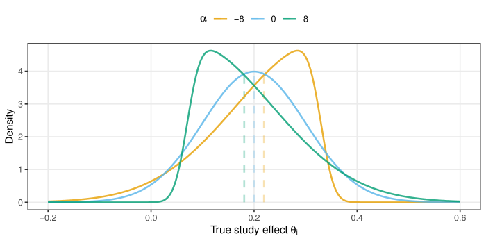
Figure 3: Illustration of skew normal distribution of true study effects $\theta_{i}$ with mean $\theta=0.2$ and variance $\tau^{2}=0.1^{2}$ for different shape parameters $\alpha$. A left-skewed distribution is obtained for $\alpha=-8$, a right-skew distribution for $\alpha=8$. The dashed lines depict the median of the corresponding distribution.

Based on a true effect $\theta_{i}$, the effect estimate $\hat{\theta}_{i}$ of study $i$ was simulated from a normal distribution

$$\hat{\theta}_{i}\sim\operatorname{N}(\theta_{i},2/n_{i}),$$

where $n_{i}$ is the (groupwise) sample size set to $n_{i}=50$ (normal studies) or $n_{i}=500$ (large studies). We considered scenarios with either $0$, $1$, or $2$ large studies (and the rest as normal studies). The corresponding squared standard error was simulated from a scaled chi-squared distribution

$$\sigma_{i}^{2}\sim\frac{1}{(n_{i}-1)n_{i}}\chi^{2}_{2(n_{i}-1)},$$

which were then transformed to standard errors by taking the square root. The heterogeneity variance $\tau^{2}$ of the study effect distribution was specified by Higgins’ $I^{2}$. Specifically, we first computed the within-study variance using

$$\epsilon^{2}=\frac{1}{k}\sum\limits_{i=1}^{k}\frac{2}{n_{i}},$$ (16)

from which we then computed the between-study heterogeneity variance by

$$\tau^{2}=\epsilon^{2}\frac{I^{2}}{1-I^{2}}$$ (17)

where $I^{2}=\tau^{2}/(\epsilon^{2}+\tau^{2})$ is Higgins’ relative heterogeneity (Higgins and Thompson, , 2002). We considered scenarios with $I^{2}=0$, $0.3$, $0.6$ or $0.9$, representing a range from no heterogeneity up to high relative heterogeneity. All manipulated factors are listed in Table 3 and were varied in a fully factorial manner, resulting in 5 (number of studies) $\times$ 3 (number of large studies) $\times$ 3 (effect distribution) $\times$ 4 (relative heterogeneity) $=180$ simulation scenarios.

Table 3: Factors considered in simulation study (varied in fully-factorial way).

Factor	Levels
Number of studies $k$	3, 5, 10, 20, 50
Number of large studies	0, 1, 2
Distribution of study-specific effects	normal, left-skew normal, right-skew normal
Higgins’ $I^{2}$	0, 0.3, 0.6, 0.9

3.3 Estimands

In meta-analysis the estimand of interest is typically the mean true study effect. However, under the assumption that the true study effects are generated from a skewed distribution, it is no longer clear whether the mean or another measure of central tendency, such as the median, should be of primary interest as the mean becomes more “atypical” with increasing skewness. Therefore, we considered both the mean and the median of the true study effect distribution as estimands of interest. For a normal study effect distribution, the mean and median are both at $\theta=0.2$, whereas for a skew normal study effect distribution, the mean is $\theta=0.2$ while the median depends on the heterogeneity and skewness, and was computed numerically using the function qsn(p = 0.5, ....) from the sn R package (Azzalini, , 2023).

3.4 Methods

Each set of simulated effect estimates and standard errors were analyzed using different methods, each producing a point estimate and a 95% confidence interval for the true effect, namely

1. Hartung-Knapp (Sidik-Jonkman) (Hartung and Knapp, , 2001; Sidik and Jonkman, , 2002)

2. Random effects meta-analysis (Borenstein et al., , 2010)

and the five $p$-value combination methods listed in Table 1. All input $p$-values were one-sided and oriented in positive effect direction (alternative "greater"). This setup exhausts all possible method/orientation combinations as Edgington’s method is orientation-invariant whereas Fisher/Pearson and Wilkinson/Tippett are orientation mirrored as described in Section 2. Each method was adjusted for potential between-study heterogeneity using the restricted maximum likelihood (REML) estimate of the heterogeneity variance $\tau^{2}$, which is usually recommended as a default choice (Langan et al., , 2019). The Hartung-Knapp and the random effects meta-analysis methods were computed with the metagen function from the R package meta (Balduzzi et al., , 2019), while the remaining $p$-value combination methods were computed with the confMeta R package (Hofmann and Held, , 2024).

3.5 Performance measures

Our primary performance measure was coverage of the 95% confidence interval which we estimated by

$$\widehat{\mathrm{Cov}}=\frac{\text{\# 95\% CI includes estimand}}{n_{\mathrm{sim}}}$$

with Monte Carlo standard error (MCSE)

$$\mathrm{MCSE}_{\widehat{\mathrm{Cov}}}=\sqrt{\frac{\widehat{\mathrm{Cov}}(1-\widehat{\mathrm{Cov}})}{n_{\mathrm{sim}}}}.$$

We conducted $n_{\mathrm{sim}}=20^{\prime}000$ simulation repetitions. This ensures a maximum Monte Carlo standard error of $0.00125\%$ (attained when the estimated coverage is 50%), which we consider as sufficiently small to detect relevant differences. Our secondary performance measures were bias (with respect to the mean and median effect) and 95% confidence interval width (see Table 3 in Siepe et al., , 2024, for definitions and MCSE formulas). To assess the skewness properties of the different methods, we computed the skewness coefficient (13) for each 95% confidence interval. We then evaluated the distribution (mean, median, minimum, maximum) of the skewness coefficients for a given method and simulation scenario. To assess the relationship between confidence interval skewness and data skewness, we also computed the Pearson correlation between the 95% confidence interval skewness $\beta$ and Fisher’s weighted skewness coefficient (12) of the meta-analyzed effect estimates with heterogeneity-adjusted weights $w_{i}=({\sigma^{2}_{i}+\hat{\tau}^{2}})^{-1}$. Finally, to assess agreement between confidence interval skewness and data skewness, we also computed Cohen’s $\kappa$ of the sign of $\gamma$ and the sign of $\beta$, using the function cohen.kappa from the psych R package (William Revelle, , 2024).

3.6 Computational aspects

The simulation study was performed using R version 4.4.0 (2024-04-24) on a server running Debian GNU/Linux 12. More information on the computational environment and code to reproduce the simulation study are available at https://github.com/felix-hof/confMeta_simulation.

3.7 Results

We will now describe the results of the simulation study. Throughout all simulation repetitions, no missing/non-convergent confidence intervals or point estimates were observed.

3.7.1 Normal study effect distribution

We first report the results based on simulation conditions with symmetric, normally distributed true study effects.

Coverage

Figure LABEL:fig:coverage shows the empirical coverage of the compared method. We see that the random effects meta-analysis (leftmost panels) has either too high (for $I^{2}=0$) or too low (for $I^{2}>0$) coverage for small numbers of studies, but seems to stabilize at the nominal 95% level as the number of studies increases. In contrast, for scenarios with no large studies (top panels), the Hartung-Knapp method shows nominal coverage over all numbers of studies, while for scenarios with one or two large studies (middle and bottom panels), the coverage is slightly too low for small numbers of studies, consistent with the results of IntHout et al., (2014). Focusing now on the $p$-value combination methods, we can see that Edgington’s method shows qualitatively similar behavior to random effects meta-analysis, but with better coverage than random effects meta-analysis in most conditions. Interestingly, Edgington’s method has even slightly better coverage than Hartung-Knapp if there are 5 or more studies, some of them being large, and $I^{2}=0.3$. The Fisher, Pearson, Wilkinson, and Tippet methods, on the other hand, often show worse coverage, which also does not stabilize at the nominal 95% but increases above as the number of studies increases.

Bias

Figure LABEL:fig:bias shows the performance of the methods in terms of bias. We see that the random effects, Hartung-Knapp, and Edgington’s methods are essentially unbiased, while Fisher’s, Pearson’s, Wilkinson’s, and Tippett’s method have substantial bias in most conditions. The bias patterns of Fisher/Pearson and Wilkinson/Tippett seem mirrored around zero, possibly because these methods’ are mirrored with respect to $p$-value orientation.

Confidence interval width

Figure LABEL:fig:width shows the average width of the method’s 95% confidence intervals. Edgington’s, Fisher’s, and Pearson’s methods have somewhat wider confidence intervals than random effects meta-analysis, while Hartung-Knapp has substantially wider intervals in conditions with a small number of studies, but all of these widths shrink and become narrower as the number of studies increases. In contrast, Wilkinson’s and Tippett’s methods seem to shrink much more slowly and remain relatively wide even with larger numbers of studies. This is even better seen in Figure 5 reported in the Appendix, which shows confidence interval width relative to the random effects meta-analysis method. We can see that the relative width of Wilkinson’s and Tippett’s methods increases, while the Hartung-Knapp and to a lesser extent Edgington’s, Fisher’s, and Pearson’s method remain constant or decrease with increasing number of studies. Interestingly, the figure also shows that the Hartung-Knapp method can have narrower confidence intervals than the random effects meta-analysis, which has been described as a potential shortcoming in the literature (Jackson et al., , 2017). In rare cases this may also happen with Edgington’s method, but only if there are no large studies and small amounts of relative heterogeneity.

Confidence interval skewness

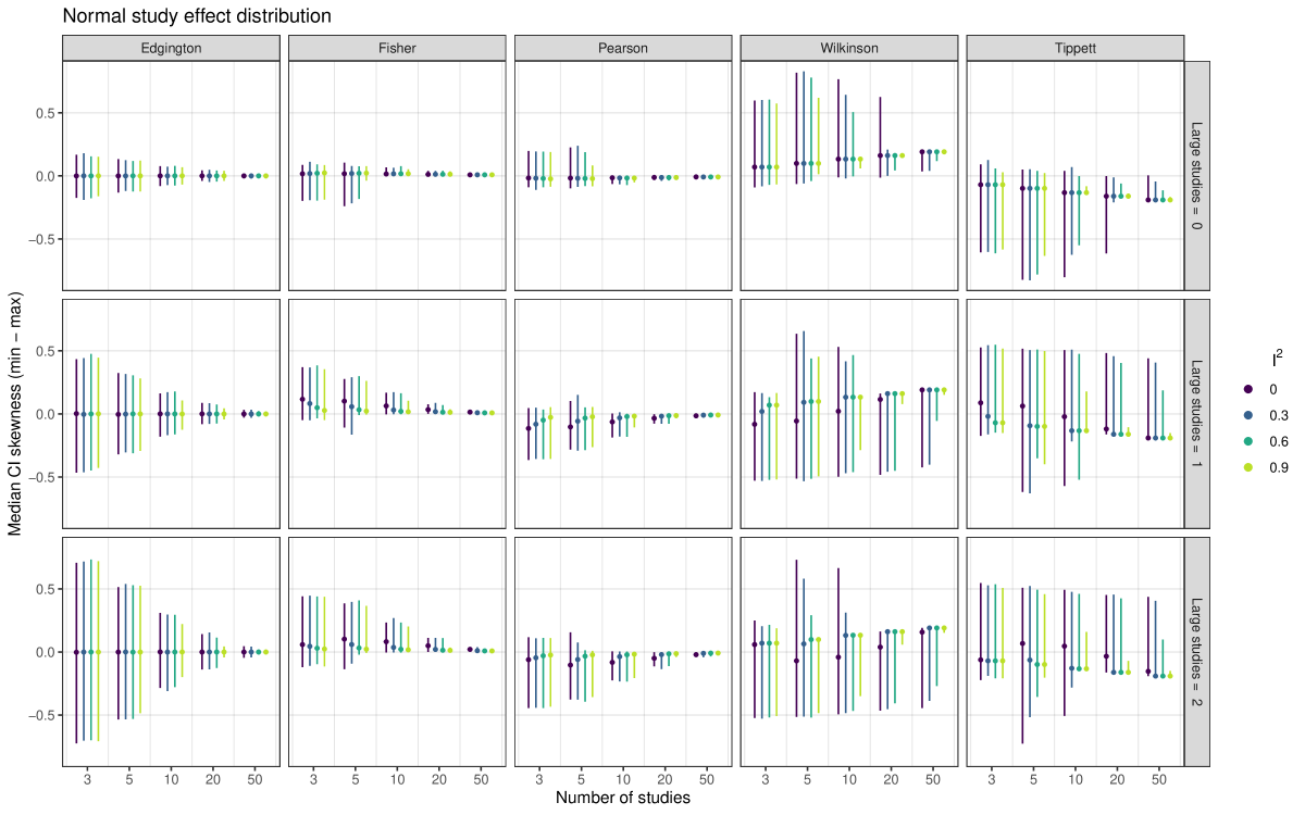
Figure 6: Skewness of 95% confidence interval based on 20’000 simulation repetitions.

Figure LABEL:fig:kappa shows the Cohen’s $\kappa$ agreement between the sign of the skewness of the confidence intervals and the skewness of the data. The random effects meta-analysis and Hartung-Knapp methods are not shown because their confidence intervals are always symmetric and thus always produce a skewness coefficient of zero. We can see that Edgington’s method shows consistently high agreement with a decreasing trend as the number of studies increases, while the other methods do show no better than chance agreement ($\kappa\approx 0$, Fisher and Pearson) or sometimes even worse than chance agreement ($\kappa<0$, Wilkinson and Tippett). Figure 6 reported in the Appendix shows the median skewness of the confidence intervals and the corresponding min-max range, illustrating why all but Edgington’s method often show exactly zero agreement: As the number of studies increases, their confidence intervals tend to be skewed in only one direction. For ten or more studies, Pearson’s method produced only confidence intervals with negative skewness, while confidence intervals based on Fisher’s method were all positively skewed. Thus, the confidence interval cannot represent the skewness type of the data, even though the confidence interval skewness tends to be correlated with the data skewness (see Figure 7 in the Appendix).

3.7.2 Skew-normal study effect distribution

Figures 8 to 25 in the Appendix show the simulation results based on the scenarios where the true study effects were simulated from left or right skew-normal distributions. The results for confidence interval width and skewness were generally similar to those from the symmetric normal scenarios, while the results for bias and coverage showed some differences which we will now discuss.

Bias

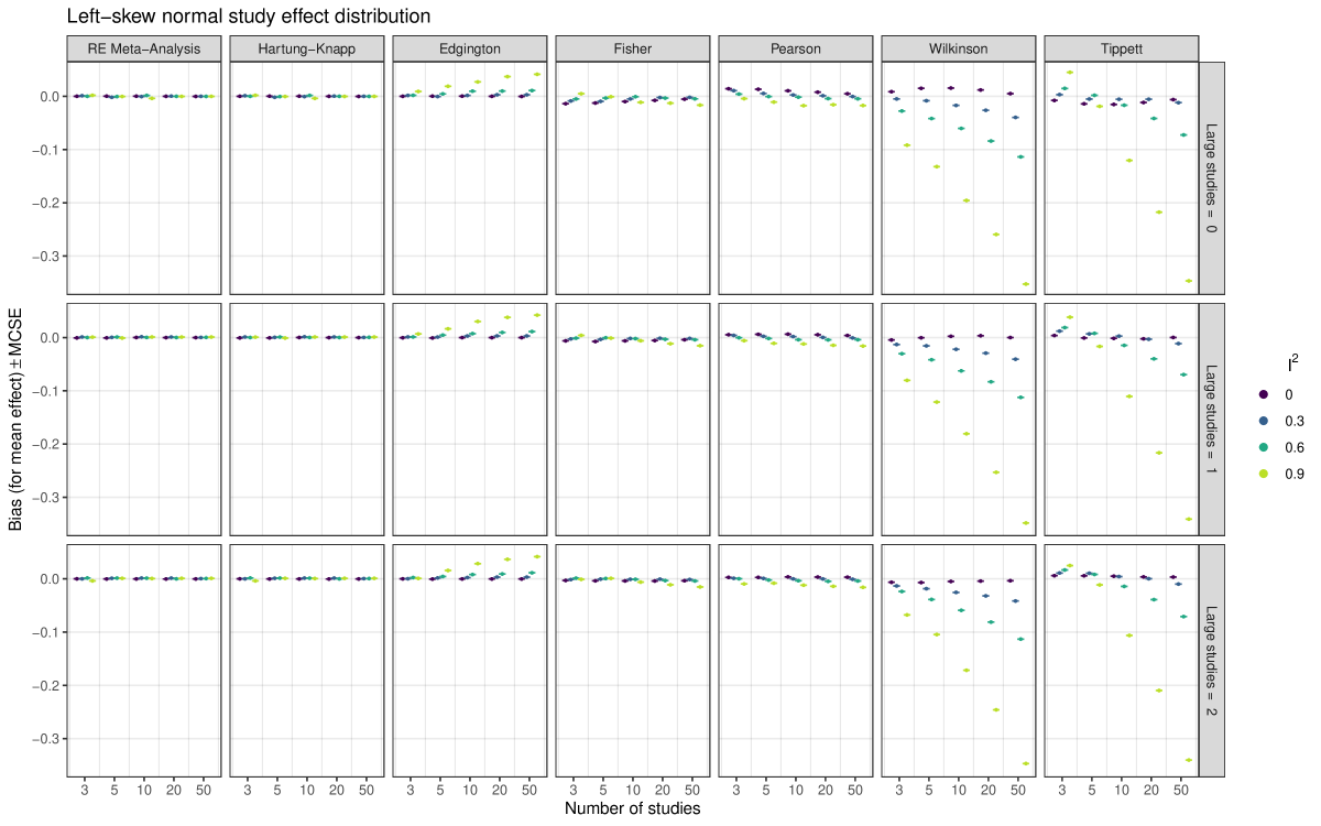
Figure 12: Empirical bias of point estimates (for mean effect) based on 20’000 simulation repetitions.

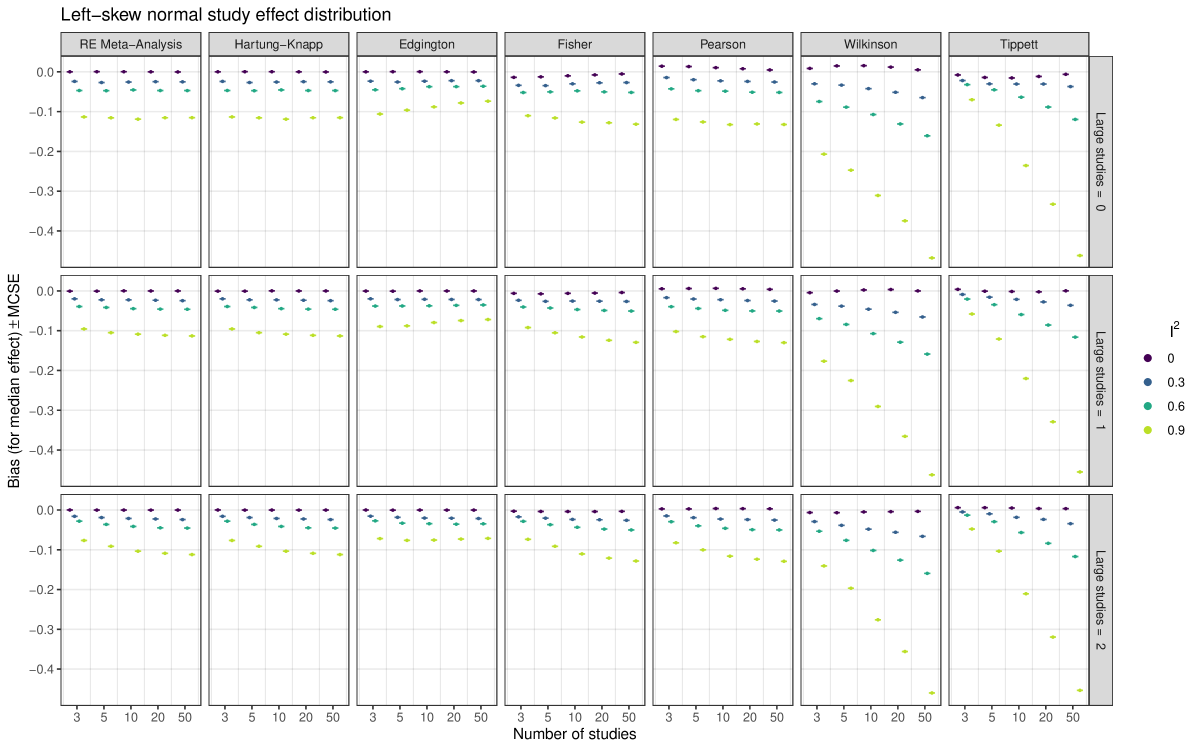
Figure 13: Empirical bias of point estimates (for median effect) based on 20’000 simulation repetitions.

As discussed earlier, we considered two estimands in the skew-normal conditions – the mean and the median of the true effect distribution. Random effects meta-analysis and the Hartung-Knapp method were unbiased for the mean effect (Figures 12 and 21) but biased for the median effect (Figures 13 and 22), with the amount of bias increasing with increasing $I^{2}$. Among the $p$-value combination methods, Wilkinson’s and Tippett’s methods were substantially biased for both the mean and median true effect, while Edgington’s, Fisher’s, and Pearson’s methods were also biased, but to a lesser extent. Interestingly, Edgington’s method appears to be positively biased for the mean effect and negatively biased for the median effect (for the left-skew condition, and vice versa for the right-skew condition), thus implicitly targeting an estimand somewhere in between the mean and median of the skew-normal distributions. Furthermore, the bias of Edgington’s method for the median effect was lower than the bias of the random effects meta-analysis and Hartung-Knapp methods.

Coverage

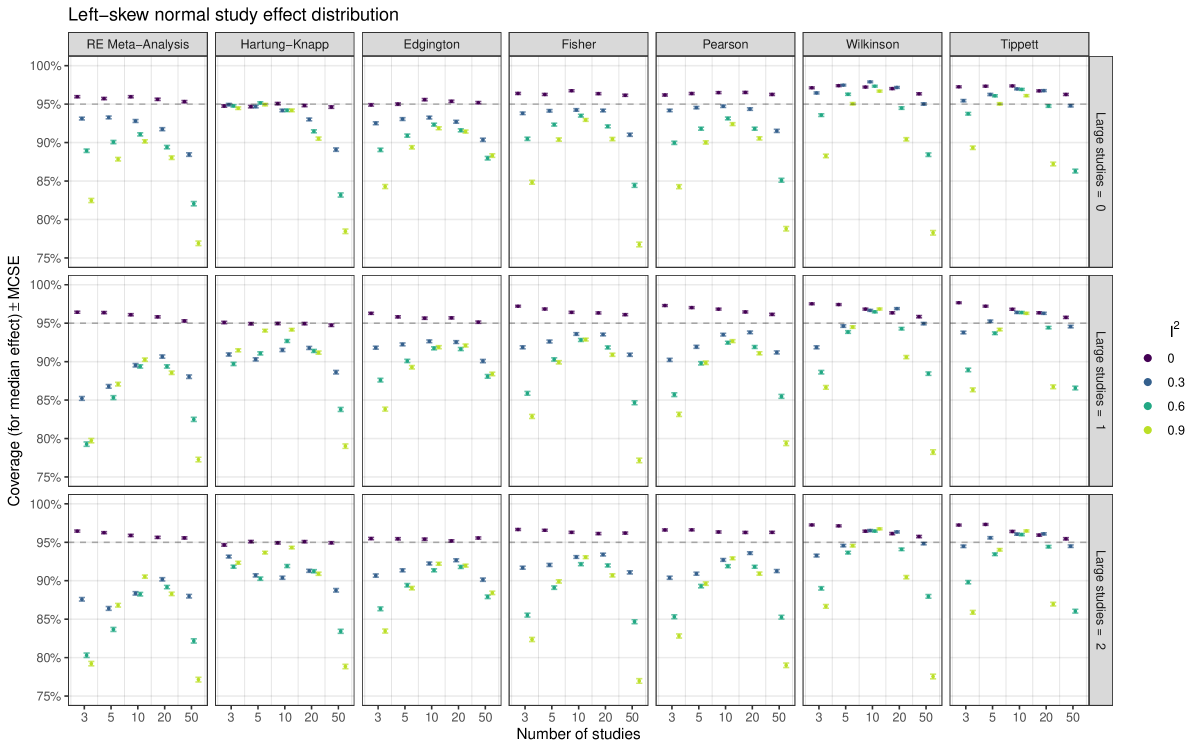
Figure 9: Empirical coverage (for median effect) of the 95% confidence intervals based on 20’000 simulation repetitions.

The random effects meta-analysis and the Hartung-Knapp method showed similar patterns of coverage for the mean effect as under symmetric-study effects conditions (Figures 8 and 17), but different patterns for the median effect (Figures 9 and 18). For the latter, their coverage did not approach the nominal 95% coverage as the number of studies increased, but actually worsened after an initial increase. This makes sense since both methods are targeting the mean rather than the median true effect, so their confidence intervals become more concentrated around the mean effect with increasing number of studies. Edgington’s method showed comparable or better coverage for the mean effect than random effects meta-analysis when $I^{2}$ was not too high, while it generally showed better (but not nominal) coverage for the median true effect. The remaining $p$-value combination methods seem to increase to too high coverage for the mean effect with increasing number of studies, and show coverage values all over the place for the median effect.

3.8 Summary of simulation results

Under symmetric study effects, Edgington’s method produced unbiased point estimates, its confidence intervals had comparable or better coverage, and were only slightly wider than the confidence intervals from a random-effects meta-analysis. In addition, it was the only method that could accurately represent data skewness. Surprisingly, however, the performance of the method was worse when study effects were simulated from a skewed distribution, possibly because the method targets neither the mean nor the median of the distribution, but something in between. The remaining $p$-value combination methods, Fisher/Pearson and, to a greater extent, Wilkinson/Tippett, could not achieve satisfactory performance. Their point estimates were more biased, their coverage for a large number of studies was too high, and their confidence intervals could not reliably represent the skewness of the data.

The Hartung-Knapp method leads to known improvements in coverage compared to random-effects meta-analysis, although nominal coverage is still not guaranteed when a meta-analysis includes a few studies that are much larger than the remaining ones (IntHout et al., , 2014). The improved coverage of the Hartung-Knapp method also comes at the cost of substantially wider confidence intervals on average, in particular if the number of studies is small (see Figure 5). In addition, our study showed that when the true study effects are simulated from a skewed distribution and the estimand is the mean study effect, both methods appear to be unbiased and show similar coverage patterns as for symmetric study effect distributions, but when the estimand of interest is the median study effect, both methods become biased and their coverage becomes worse.

4 Discussion and extensions

We have compared different $p$-value combination methods for meta-analysis theoretically and through simulation. Adjustments for heterogeneity have been made based on the standard additive approach. Alternatively multiplicative heterogeneity can be incorporated, where the squared standard errors $\sigma_{i}^{2}$ are multiplied with a factor $\phi>0$. Then we would use the adjusted $z$-statistic

$$Z_{i}=\frac{\hat{\theta}_{i}-\mu}{\sqrt{\hat{\phi}}\,\sigma_{i}}$$

where $\hat{\phi}=\max\{Q/(k-1),1\}$ is the appropriate overdispersion estimate (Stanley and Doucouliagos, , 2015; Mawdsley et al., , 2017). However, both additive and multiplicative adjustments are based on a plug-in approach, which ignores the uncertainty of the heterogeneity estimate $\hat{\tau}^{2}$ and $\hat{\phi}$, respectively. An interesting alternative would be to profile-out the heterogeneity parameter, see Cunen and Hjort, (2021) and Zabriskie et al., (2021).

A possible extension of the method provided is cumulative meta-analysis, where studies are added one at a time in a specific order, usually time of publication (Egger et al., , 2022). It will be interesting to compare the width of the confidence interval with the length of the standard random effects confidence interval as the data accumulates. It may also be worthwhile to conduct a simulation study with focus on error rates, as standard random effects cumulative meta-analysis is prone to Type-I error rate inflation (ter Schure and Grünwald, , 2019; Kulinskaya and Mah, , 2022), which may result in too narrow confidence intervals.

To summarize, the $p$-value function approach based on Edgington combination method constitutes a promising avenue for further research and applications. Its ability to reflect the skewness of the data will be attractive to applied meta-analysts. It may also be useful for applications in health technology assessment with a small number of studies, where a Bayesian approach has recently been proposed as an alternative to the “overly conservative” Hartung-Knapp method (Lilienthal et al., , 2024).

It would also be interesting to extend the approach to compute prediction intervals for future study effects (Higgins et al., , 2009; Hamaguchi et al., , 2021; Nagashima et al., , 2019). This would involve numerical integration of a $\operatorname{N}(\mu,\tau^{2})$ distribution with respect to the confidence density for $\mu$, which can be obtained from any (monotonically increasing) one-sided $p$-value through differentiation. For example, differentiation of the underlying exact one-sided $p$-value function from Figure 2 gives the confidence density shown in Figure 4. The confidence density is clearly skewed, which would then also be the case for the corresponding prediction interval. We plan to consider this in future work.

Figure 4: Confidence density based on Edgington’s combined $p$-value function and exact $p$-values with mid-$p$ correction for meta-analysis of $n=7$ randomized controlled clinical trials investigating the association between corticosteroids and mortality in hospitalized patients with COVID-19 (WHO REACT Working Group, , 2020).

Data and Software Availability

Meta-analysis with $p$-value combination methods is implemented in the R-package confMeta available on GitHub (https://github.com/felix-hof/confMeta). The package will be soon submitted to CRAN. R code to reproduce our results is available at https://osf.io/je8xb/. R code to reproduce the simulation study is available at https://github.com/felix-hof/confMeta_simulation.

Funding

Partial support by the Swiss National Science Foundation (Project # 189295) is gratefully acknowledged.

Conflict of Interest Statement

The authors declare that no conflict of interest exists for all authors.

Appendix A Relationships of p-value combination methods

A.1 Edgington’s method

Define

$$\overset{\leftharpoonup}{s}=\sum_{i=1}^{n}\overset{\leftharpoonup}{p_{i}}=\sum_{i=1}^{n}(1-\overset{\rightharpoonup}{p_{i}})=n-\sum_{i=1}^{n}\overset{\rightharpoonup}{p_{i}}=n-\overset{\rightharpoonup}{s},$$

so $\overset{\rightharpoonup}{p_{E}}=\Pr(\mathrm{I}_{n}\leq\overset{\rightharpoonup}{s})=1-\Pr(\mathrm{I}_{n}>\overset{\rightharpoonup}{s})$ where $\mathrm{I}_{n}\in[0,n]$ is an Irwin-Hall random variable with parameter $n$. Since the Irwin-Hall distribution is symmetric around its mean $n/2$, it holds that $\Pr(\mathrm{I}_{n}\leq{s})=\Pr(\mathrm{I}_{n}>n-{s})$ for any $s\in[0,n]$. Hence, it follows that

$$\overset{\rightharpoonup}{p}_{E} = \Pr(\mathrm{I}_{n}\leq\overset{\rightharpoonup}{s})$$

$$= \Pr(\mathrm{I}_{n}>n-\overset{\rightharpoonup}{s})$$

$$= \Pr(\mathrm{I}_{n}>\overset{\leftharpoonup}{s})$$

$$= 1-\Pr(\mathrm{I}_{n}\leq\overset{\leftharpoonup}{s})$$

$$= 1-\overset{\leftharpoonup}{p}_{E}.$$

A.2 Fisher’s and Pearson’s methods

Define

$$\overset{\rightharpoonup}{f}=-2\sum_{i=1}^{n}\log(\overset{\rightharpoonup}{p_{i}})=-2\sum_{i=1}^{n}\log(1-\overset{\leftharpoonup}{p_{i}})=\overset{\leftharpoonup}{k}.$$

It follows that

$$\overset{\rightharpoonup}{p}_{F} = \Pr(\chi_{2n}^{2}>\overset{\rightharpoonup}{f})$$

$$= \Pr(\chi_{2n}^{2}>\overset{\leftharpoonup}{k})$$

$$= 1-\Pr(\chi_{2n}^{2}\leq\overset{\leftharpoonup}{k})$$

$$= 1-\overset{\leftharpoonup}{p}_{P}.$$

Similarly we obtain $\overset{\rightharpoonup}{p}_{P}=1-\overset{\leftharpoonup}{p}_{F}$.

A.3 Tippett’s and Wilkinson’s methods

We have

$$\overset{\rightharpoonup}{p}_{T} = 1-(1-\min\{\overset{\rightharpoonup}{p_{1}},\dots,\overset{\rightharpoonup}{p_{n}}\})^{n}$$

$$= 1-(1-\min\{1-\overset{\leftharpoonup}{p_{1}},\dots,1-\overset{\leftharpoonup}{p_{n}}\})^{n}$$

$$= 1-\max\{\overset{\leftharpoonup}{p_{1}},\dots,\overset{\leftharpoonup}{p_{n}}\}^{n}$$

$$= 1-\overset{\leftharpoonup}{p}_{W}$$

and similarly $\overset{\rightharpoonup}{p}_{W}=1-\overset{\leftharpoonup}{p}_{T}$.

Appendix B Additional simulation results

The following figures show additional simulation results under a normal study effect distribution (Figure 5-7), a left-skew normal study effect distribution (Figure 8-16), and a right-skew normal study effect distribution (Figure 17-25).

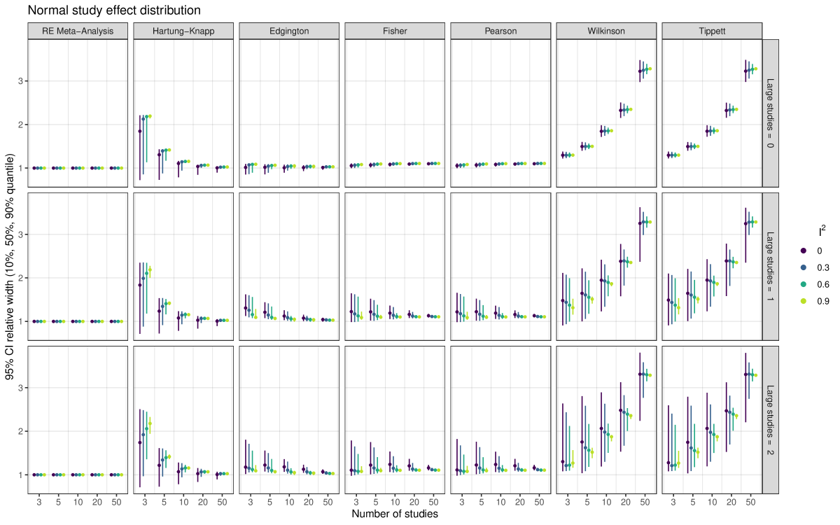
Figure 5: Relative width of 95% confidence intervals (relative to random effects meta-analysis) based on 20’000 simulation repetitions.

Figure 7: Correlation between 95% confidence interval skewness and data skewness based on 20’000 simulation repetitions.

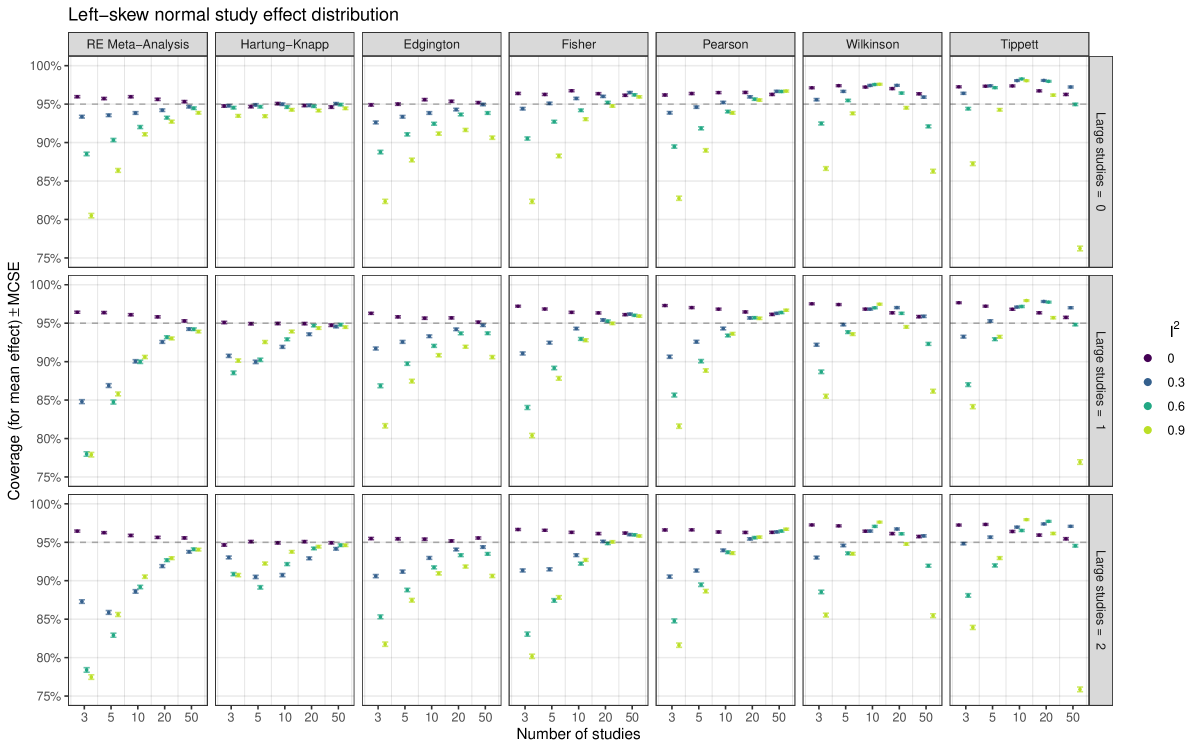
Figure 8: Empirical coverage (for mean effect) of the 95% confidence intervals based on 20’000 simulation repetitions.

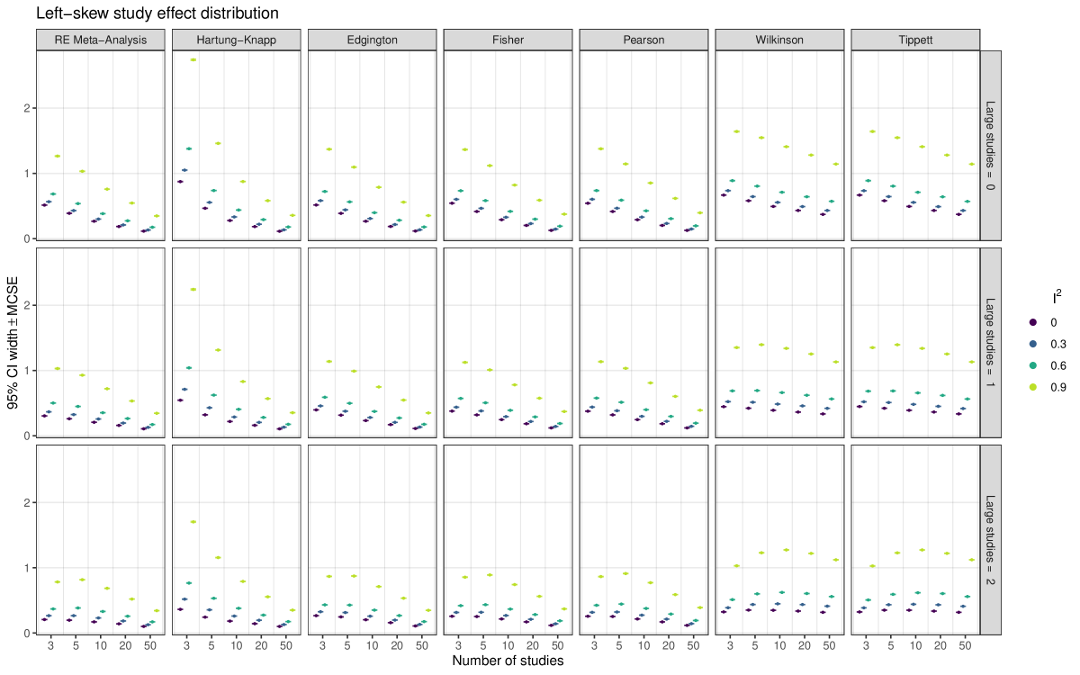
Figure 10: Mean width of 95% confidence intervals based on 20’000 simulation repetitions.

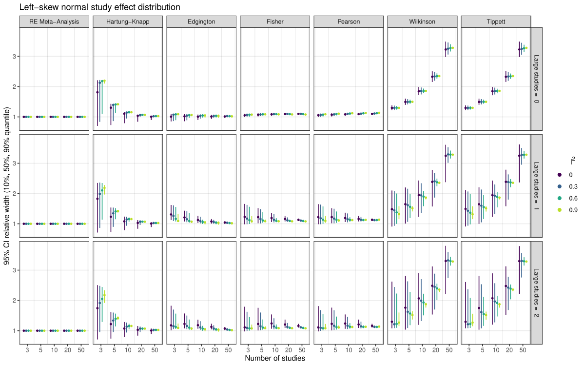
Figure 11: Relative width of 95% confidence intervals (relative to random effects meta-analysis) based on 20’000 simulation repetitions.

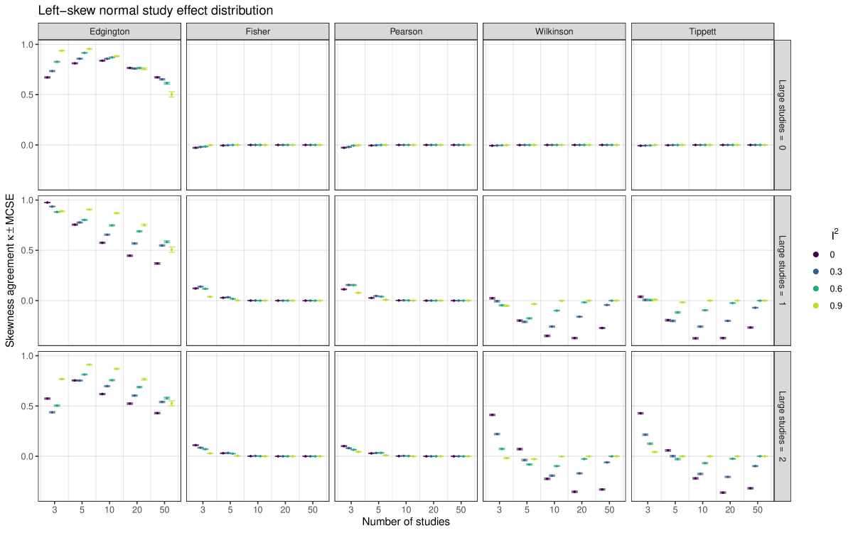
Figure 14: Cohen’s $\kappa$ sign agreement between 95% confidence interval skewness and data skewness based on 20’000 simulation repetitions.

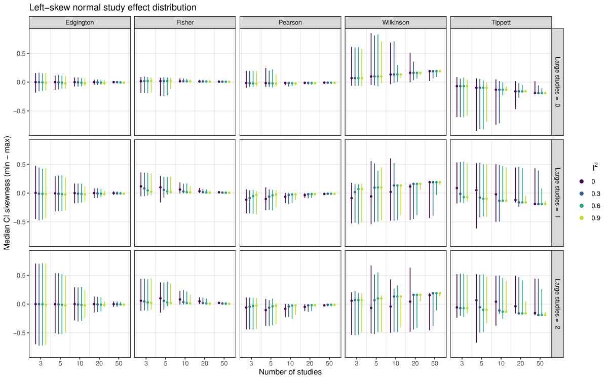
Figure 15: Skewness of 95% confidence intervals based on 20’000 simulation repetitions.

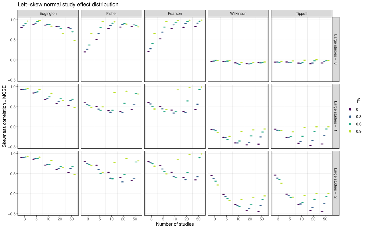
Figure 16: Correlation between 95% confidence interval skewness and data skewness based on 20’000 simulation repetitions.

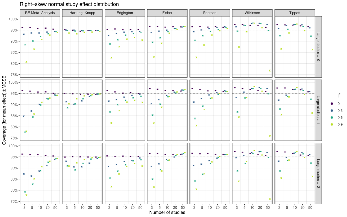
Figure 17: Empirical coverage (for mean effect) of the 95% confidence intervals based on 20’000 simulation repetitions.

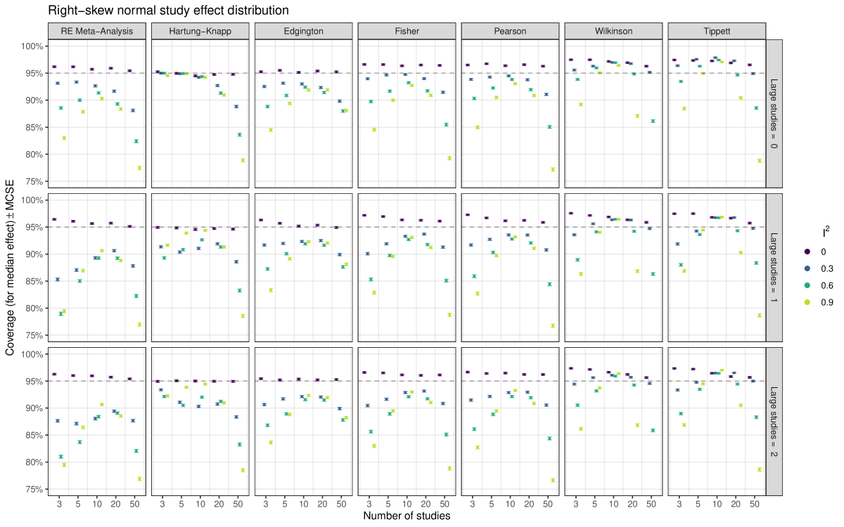
Figure 18: Empirical coverage (for median effect) of the 95% confidence intervals based on 20’000 simulation repetitions.

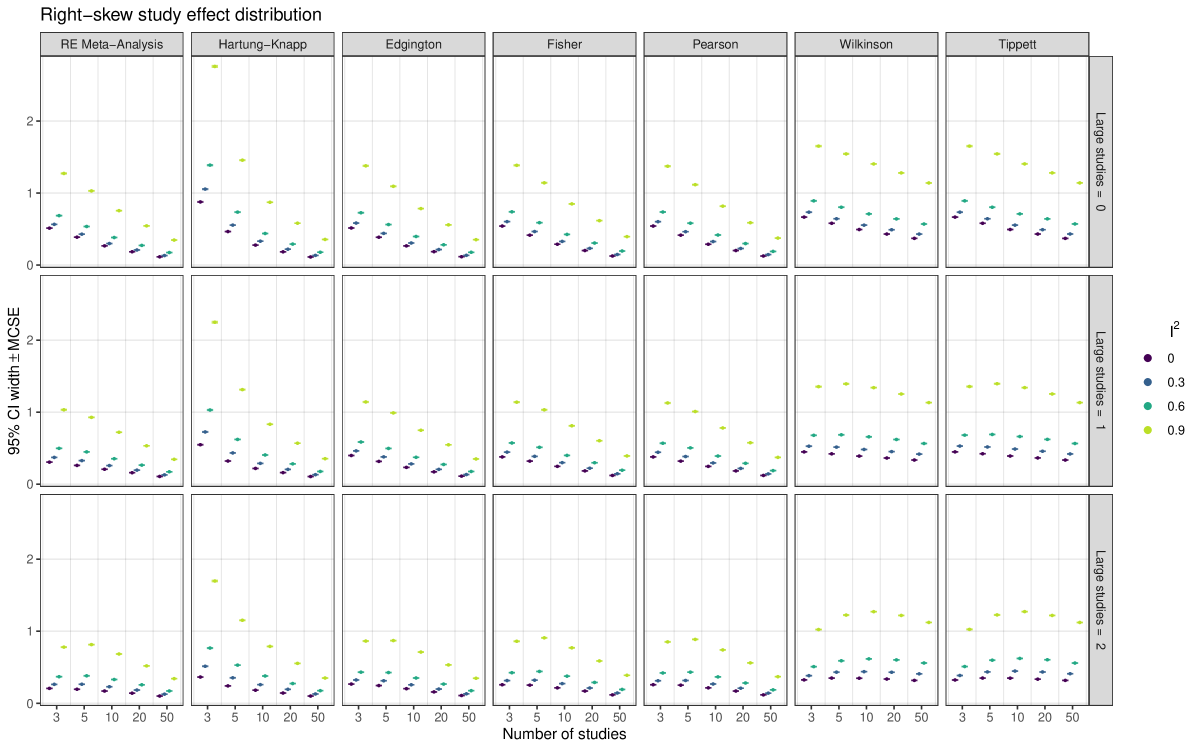
Figure 19: Mean width of 95% confidence intervals based on 20’000 simulation repetitions.

Figure 20: Relative width of 95% confidence intervals (relative to random effects meta-analysis) based on 20’000 simulation repetitions.

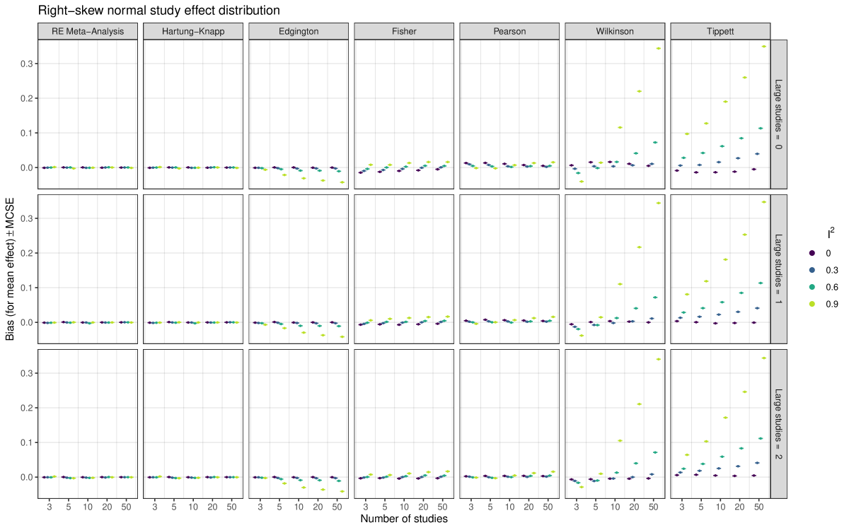
Figure 21: Empirical bias of point estimates (for mean effect) based on 20’000 simulation repetitions.

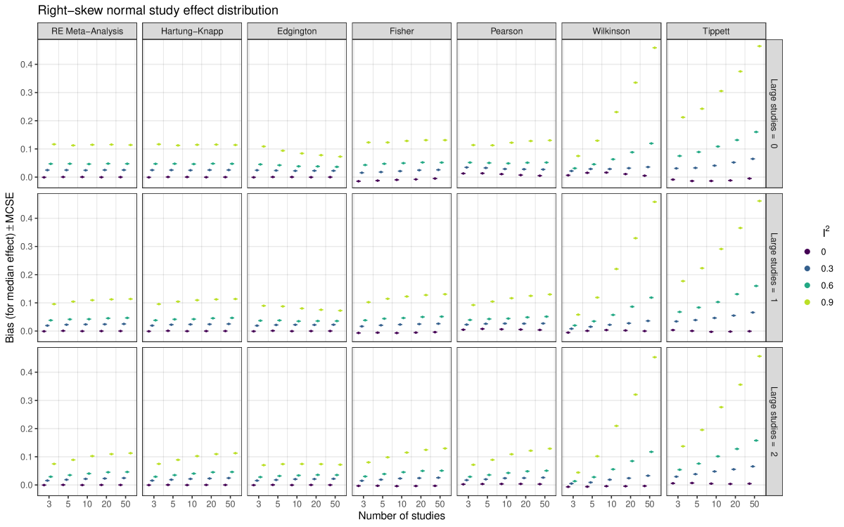
Figure 22: Empirical bias of point estimates (for median effect) based on 20’000 simulation repetitions.

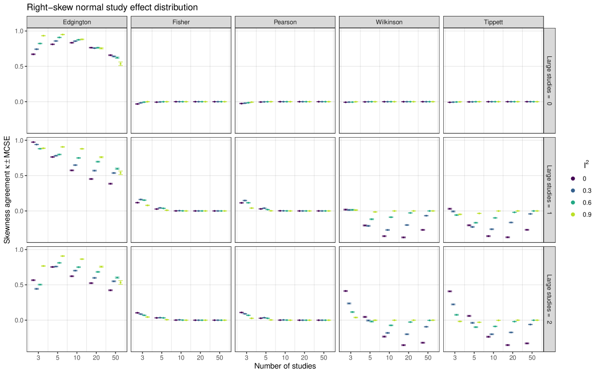
Figure 23: Cohen’s $\kappa$ sign agreement between 95% confidence interval skewness and data skewness based on 20’000 simulation repetitions.

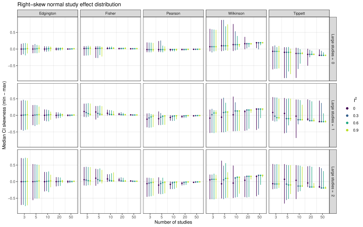
Figure 24: Skewness of 95% confidence intervals based on 20’000 simulation repetitions.

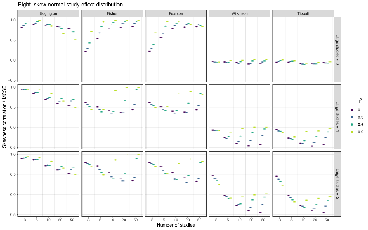
Figure 25: Correlation between 95% confidence interval skewness and data skewness based on 20’000 simulation repetitions.

References

- Azzalini and Capitanio, (2013) Azzalini, A. and Capitanio, A. (2013). The Skew-Normal and Related Families. Cambridge University Press.
- Azzalini, (2023) Azzalini, A. A. (2023). The R package sn: The skew-normal and related distributions such as the skew- and the SUN (version 2.1.1). Università degli Studi di Padova, Italia. Home page: http://azzalini.stat.unipd.it/SN/.
- Balduzzi et al., (2019) Balduzzi, S., Rücker, G., and Schwarzer, G. (2019). How to perform a meta-analysis with R: a practical tutorial. Evidence-Based Mental Health, (22):153–160.
- Bender et al., (2005) Bender, R., Berg, G., and Zeeb, H. (2005). Tutorial: Using confidence curves in medical research. Biometrical Journal, 47(2):237–247.
- Borenstein et al., (2010) Borenstein, M., Hedges, L. V., Higgins, J. P., and Rothstein, H. R. (2010). A basic introduction to fixed-effect and random-effects models for meta-analysis. Research Synthesis Methods, 1(2):97–111.
- Cochran, (1937) Cochran, W. (1937). Problems arising in the analysis of a series of similar experiments. Journal of the Royal Statistical Society, 4(1):102–118.
- Cousins, (2007) Cousins, R. D. (2007). Annotated bibliography of some papers on combining significances or p-values. https://arxiv.org/abs/0705.2209.
- Cunen and Hjort, (2021) Cunen, C. and Hjort, N. L. (2021). Combining information across diverse sources: The II-CC-FF paradigm. Scandinavian Journal of Statistics, 49(2):625–656.
- DerSimonian and Laird, (1986) DerSimonian, R. and Laird, N. (1986). Meta-analysis in clinical trials. Controlled Clinical Trials, 7(3):177–188.
- (10) Edgington, E. S. (1972a). An additive method for combining probability values from independent experiments. The Journal of Psychology, 80(2):351–363.
- (11) Edgington, E. S. (1972b). A normal curve method for combining probability values from independent experiments. The Journal of Psychology, 82(1):85–89.
- Egger et al., (2022) Egger, M., Higgins, J. P. T., and Smith, G. D. (2022). Systematic Reviews in Health Research – Meta-Analysis in Context. John Wiley & Sons, Hoboken, NJ, third edition.
- Fisher, (1932) Fisher, R. A. (1932). Statistical Methods for Research Workers. Oliver & Boyd, Edinburgh, 4 edition.
- Fraser, (2017) Fraser, D. A. S. (2017). -values: The insight to modern statistical inference. Annual Review of Statistics and its Application, 4:1–14.
- Fraser, (2019) Fraser, D. A. S. (2019). The -value function and statistical inference. The American Statistician, 73(sup1):135–147.
- Groeneveld and Meeden, (1984) Groeneveld, R. A. and Meeden, G. (1984). Measuring skewness and kurtosis. The Statistician, 33(4):391.
- Hall, (1927) Hall, P. (1927). The distribution of means for samples if size drawn from a population in which the variate takes values between 0 and 1, all such values being equally probable. Biometrika, 19(3-4):240–244.
- Hamaguchi et al., (2021) Hamaguchi, Y., Noma, H., Nagashima, K., Yamada, T., and Furukawa, T. A. (2021). Frequentist performances of bayesian prediction intervals for random-effects meta-analysis. Biometrical Journal, 63(2):394–405.
- Hartung and Knapp, (2001) Hartung, J. and Knapp, G. (2001). A refined method for the meta-analysis of controlled clinical trials with binary outcome. Statistics in Medicine, 20(24):3875–3889.
- Hedges and Olkin, (1985) Hedges, L. V. and Olkin, I. (1985). Statistical Methods for Meta-Analysis. Elsevier.
- Henmi and Copas, (2010) Henmi, M. and Copas, J. B. (2010). Confidence intervals for random effects meta-analysis and robustness to publication bias. Statistics in Medicine, 29:2969–2983.
- Higgins and Thompson, (2002) Higgins, J. P. T. and Thompson, S. G. (2002). Quantifying heterogeneity in a meta-analysis. Statistics in Medicine, 21(11):1539–1558.
- Higgins et al., (2009) Higgins, J. P. T., Thompson, S. G., and Spiegelhalter, D. J. (2009). A re-evaluation of random-effects meta-analysis. Journal of the Royal Statistical Society: Series A (Statistics in Society), 172(1):137–159.
- Higgins et al., (2008) Higgins, J. P. T., White, I. R., and Anzures-Cabrera, J. (2008). Meta-analysis of skewed data: Combining results reported on log-transformed or raw scales. Statistics in Medicine, 27(29):6072–6092.
- Hofmann and Held, (2024) Hofmann, F. and Held, L. (2024). confMeta: Confidence Curves and P-Value Functions for Meta-Analysis. R package version 0.3.1.
- Infanger and Schmidt-Trucksäss, (2019) Infanger, D. and Schmidt-Trucksäss, A. (2019). P value functions: An underused method to present research results and to promote quantitative reasoning. Statistics in Medicine, 38(21):4189–4197.
- IntHout et al., (2014) IntHout, J., Ioannidis, J. P., and Borm, G. F. (2014). The Hartung-Knapp-Sidik-Jonkman method for random effects meta-analysis is straightforward and considerably outperforms the standard DerSimonian-Laird method. BMC Medical Research Methodology, 14.
- Irwin, (1927) Irwin, J. O. (1927). On the frequency distribution of the means of samples from a population having any law of frequency with finite moments, with special reference to Pearson’s Type II. Biometrika, 19(3-4):225–239.
- Jackson et al., (2017) Jackson, D., Law, M., Rücker, G., and Schwarzer, G. (2017). The Hartung-Knapp modification for random-effects meta-analysis: A useful refinement but are there any residual concerns? Statistics in Medicine, 36(25):3923–3934.
- Kulinskaya and Mah, (2022) Kulinskaya, E. and Mah, E. Y. (2022). Cumulative meta-analysis: What works. Research Synthesis Methods, 13(1):48–67.
- Lancaster, (1961) Lancaster, H. O. (1961). Significance tests in discrete distributions. Journal of the American Statistical Association, 56(294):223–234.
- Langan et al., (2019) Langan, D., Higgins, J. P., Jackson, D., Bowden, J., Veroniki, A. A., Kontopantelis, E., Viechtbauer, W., and Simmonds, M. (2019). A comparison of heterogeneity variance estimators in simulated random-effects meta-analyses. Research Synthesis Methods, 10(1):83–98.
- Lilienthal et al., (2024) Lilienthal, J., Sturtz, S., Schürmann, C., Maiworm, M., Röver, C., Friede, T., and Bender, R. (2024). Bayesian random-effects meta-analysis with empirical heterogeneity priors for application in health technology assessment with very few studies. Research Synthesis Methods, 15(2):275–287.
- Liu et al., (2014) Liu, D., Liu, R. Y., and Xie, M. (2014). Exact meta-analysis approach for discrete data and its application to 2 × 2 tables with rare events. Journal of the American Statistical Association, 109(508):1450–1465.
- Marschner, (2024) Marschner, I. C. (2024). Confidence distributions for treatment effects in clinical trials: Posteriors without priors. Statistics in Medicine, 43(6):1271–1289.
- Mawdsley et al., (2017) Mawdsley, D., Higgins, J. P. T., Sutton, A. J., and Abrams, K. R. (2017). Accounting for heterogeneity in meta-analysis using a multiplicative model—an empirical study. Research Synthesis Methods, 8(1):43–52.
- Melilli and Veronese, (2024) Melilli, E. and Veronese, P. (2024). Confidence distributions and hypothesis testing. Statistical Papers, 65(6):3789–3820.
- Morris et al., (2019) Morris, T. P., White, I. R., and Crowther, M. J. (2019). Using simulation studies to evaluate statistical methods. Statistics in Medicine, 38(11):2074–2102.
- Nagashima et al., (2019) Nagashima, K., Noma, H., and Furukawa, T. A. (2019). Prediction intervals for random-effects meta-analysis: A confidence distribution approach. Statistical Methods in Medical Research, 28(6):1689–1702. PMID: 29745296.
- Pearson, (1933) Pearson, K. (1933). On a method of determining whether a sample of size n supposed to have been drawn from a parent population having a known probability integral has probably been drawn at random. Biometrika, 25:379–410.
- Rice et al., (2018) Rice, K., Higgins, J. P. T., and Lumley, T. (2018). A re-evaluation of fixed effect(s) meta-analysis. Journal of the Royal Statistical Society: Series A (Statistics in Society), 181(1):205–227.
- Rücker and Schwarzer, (2020) Rücker, G. and Schwarzer, G. (2020). Beyond the forest plot: The drapery plot. Research Synthesis Methods, 12(1):13–19.
- Senn, (2021) Senn, S. (2021). Statistical Issues in Drug Development. Wiley. https://doi.org/10.1002/9781119238614.
- Sidik and Jonkman, (2002) Sidik, K. and Jonkman, J. N. (2002). A simple confidence interval for meta-analysis. Statistics in Medicine, 21(21):3153–3159.
- Siepe et al., (2024) Siepe, B. S., Bartoš, F., Morris, T. P., Boulesteix, A.-L., Heck, D. W., and Pawel, S. (2024). Simulation studies for methodological research in psychology: A standardized template for planning, preregistration, and reporting. Psychological Methods. To appear. https://doi.org/10.31234/osf.io/ufgy6.
- Singh et al., (2005) Singh, K., Xie, M., and Strawderman, W. E. (2005). Combining information from independent sources through confidence distributions. The Annals of Statistics, 33(1).
- Stanley and Doucouliagos, (2015) Stanley, T. D. and Doucouliagos, H. (2015). Neither fixed nor random: weighted least squares meta-analysis. Statistics in Medicine, 34(13):2116–2127.
- Stouffer et al., (1949) Stouffer, S. A., Suchman, E. A., Devinney, L. C., Star, S. A., and Williams, R. M., J. (1949). The American soldier: Adjustment during army life. (Studies in social psychology in World War II). Cambridge University Press, Princeton Univ. Press.
- ter Schure and Grünwald, (2019) ter Schure, J. and Grünwald, P. (2019). Accumulation bias in meta-analysis: the need to consider time in error control. F1000Research, 8(962).
- Tippett, (1931) Tippett, L. H. C. (1931). Methods of Statistics. Williams Norgate.
- WHO REACT Working Group, (2020) WHO REACT Working Group (2020). Association between administration of systemic corticosteroids and mortality among critically ill patients with COVID-19: A meta-analysis. JAMA, 324(13):1330–1341.
- Wilkinson, (1951) Wilkinson, B. (1951). A statistical consideration in psychological research. Psychological Bulletin, 48:156–158.
- William Revelle, (2024) William Revelle (2024). psych: Procedures for Psychological, Psychometric, and Personality Research. Northwestern University, Evanston, Illinois. R package version 2.4.3.
- Xie et al., (2011) Xie, M., Singh, K., and Strawderman, W. E. (2011). Confidence distributions and a unifying framework for meta-analysis. Journal of the American Statistical Association, 106(493):320–333.
- Yang et al., (2016) Yang, G., Liu, D., Wang, J., and Xie, M.-G. (2016). Meta-analysis framework for exact inferences with application to the analysis of rare events. Biometrics, 72(4):1378–1386.
- Zabriskie et al., (2021) Zabriskie, B. N., Corcoran, C., and Senchaudhuri, P. (2021). A comparison of confidence distribution approaches for rare event meta-analysis. Statistics in Medicine, 40(24):5276–5297.