Nonperturbative four-gluon vertex in soft kinematics

Abstract

We present a nonperturbative study of the form factor associated with the projection of the full four-gluon vertex on its classical tensor, for a set of kinematics with one vanishing and three arbitrary external momenta. The treatment is based on the Schwinger-Dyson equation governing this vertex, and a large-volume lattice simulation, involving ten thousand gauge field configurations. The key hypothesis employed in both approaches is the “planar degeneracy”, which classifies diverse configurations by means of a single variable, thus enabling their meaningful “averaging”. The results of both approaches show notable agreement, revealing a considerable suppression of the averaged form factor in the infrared. The deviations from the exact planar degeneracy are discussed in detail, and a supplementary variable is used to achieve a more accurate description. The effective charge defined through this special form factor is computed within both approaches, and the results obtained are in excellent agreement.

1 Introduction

In the last decades our comprehension of Quantum Chromodynamics (QCD)  [1, 2, 3, 4] has improved substantially due to the ongoing exploration of basic correlation functions of the theory, such as propagators and vertices [5, 6, 7, 8, 9, 10, 11, 12, 13, 14]. This systematic survey is advancing thanks to studies based on nonperturbative methods formulated in the continuum, such as Schwinger-Dyson equations (SDEs) [5, 6, 7, 15, 8, 9, 10, 11, 12, 13, 16, 17, 18, 19, 20, 21, 22, 23, 24, 25, 14], the functional renormalization group [26, 27, 28, 29, 30, 31, 32, 33, 34, 35, 36], or models that incorporate certain key aspects of the theory [37, 38, 39, 40, 41, 42]. In addition, large-volume gauge-fixed lattice simulations [43, 44, 45, 46, 47, 48, 49, 50, 51, 52, 53, 54, 55, 56, 57, 58, 59, 60] provide invaluable insights into the evolution of correlation functions at intermediate and low values of their physical momenta. This combined information is essential for the veracious computation of physical observables [9, 61, 11, 62, 63, 36, 64], and the scrutiny of the theoretical underpinnings of non-Abelian gauge theories  [65, 66, 67, 68, 69, 70, 71, 72, 73].

Whereas the two- and three-point sectors of QCD have been the focal point of intense investigation, the nonperturbative features of the four-gluon vertex, ${\rm{I}}\!\Gamma^{abcd}_{\mu\nu\rho\sigma}(q,r,p,t)$, remain largely unexplored; for perturbative results, see [74, 75, 76, 77, 78, 79, 80, 81]. The main obstacle in the continuum is the proliferation of Lorentz and color structures, while on the lattice the statistical noise increases considerably as one advances from three to four gluon legs. As a result, both SDE studies [82, 24, 83] and lattice simulations [84] have been restricted to simple kinematic setups, where the logistic complexity is vastly reduced; such are the “collinear” configurations, where all momenta are parallel.

In the present work we carry out a comprehensive study of the four-gluon vertex for a considerably wider set of kinematics. In particular, we consider the case where one momentum vanishes ($t=0$), while the space-like momenta $q$, $r$, and $p$ are arbitrary; we will refer to these configurations as “soft kinematics”.

Our analysis is based on the synergy between two distinct nonperturbative approaches: the SDE governing the evolution of this vertex, and gauge-fixed simulations performed on large-volume lattices. In both cases, the computations are carried out in the Landau gauge.

The central theme of our considerations is the property of “planar degeneracy” [85], which has been extensively studied in the context of the three-gluon vertex  [86, 87, 88]. In the case of the four gluon vertex, this property affirms that the form factor associated with the classical tensor is approximately equal for all configurations lying on the plane $\bar{s}^{2}=(q^{2}+r^{2}+p^{2}+t^{2})/2$, or, in the soft kinematics, $s^{2}=(q^{2}+r^{2}+p^{2})/2$. Even though not exact, this feature is particularly useful on the lattice, because configurations with the same $s^{2}$ are treated as equivalent; thus, seemingly unrelated measurements are summed up and averaged, leading to a vast improvement of the signal.

The averaged form factor extracted from the lattice displays a clear infrared suppression with respect to its tree-level value (unity), in qualitative agreement with previous continuum studies performed in other kinematic configurations [82, 24, 83, 42]. Moreover, it is in very good agreement with the corresponding result obtained from a detailed SDE analysis in the soft kinematics, where the assumption of the planar degeneracy has been employed in order to simplify the iterative procedure.

The deviation of the result from the exact planar degeneracy is quantified in terms of an additional kinematic parameter, which, in conjunction with $s^{2}$, allows for a more accurate description of the underlying dynamics.

Finally, the renormalization-group invariant (RGI) effective charge corresponding to this interaction is constructed, using the lattice and the SDE results; the two curves so obtained show excellent agreement.

2 General structure and kinematics

The correlation function composed out of four gauge fields at momenta $q$, $r$, $p$, and $t$ (with $q+r+p+t=0$), is defined as

$$\mathcal{G}_{\mu\nu\rho\sigma}^{abcd}(q,r,p,t)=\langle\widetilde{A}_{\mu}^{a}(q)\widetilde{A}_{\nu}^{b}(r)\widetilde{A}_{\rho}^{c}(p)\widetilde{A}_{\sigma}^{d}(t)\rangle\;,$$ (1)

where $\widetilde{A}_{\mu}^{a}(q)$ are the SU(3) gauge fields in Fourier space, and the average $\langle.\rangle$ indicates functional integration over the gauge space (Monte Carlo average in lattice QCD). The function $\mathcal{G}_{\mu\nu\rho\sigma}^{abcd}(q,r,p,t)$ contains a connected part, denoted $\mathcal{\widetilde{C}}^{abcd}_{\mu\nu\rho\sigma}$, and disconnected propagator-like contributions. Additionally, the amputated vertex $\mathcal{C}^{abcd}_{\mu\nu\rho\sigma}$ can be further separated into one-particle irreducible (1PI) and one-particle reducible (1PR) parts, denoted respectively ${\rm{I}}\!\Gamma^{abcd}_{\mu\nu\rho\sigma}$ and $\mathbb{V}^{abcd}_{\mu\nu\rho\sigma}$, as shown in Fig. 1. At tree-level, ${\rm{I}}\!\Gamma^{abcd}_{\mu\nu\rho\sigma}\to\Gamma^{abcd}_{0\,\mu\nu\rho\sigma}$, see, e.g., Eq. (2.11) in [83].

In the Landau gauge that we employ throughout, the gluon propagator, $\Delta_{\mu\nu}^{ab}(q)=-i\delta^{ab}\Delta_{\mu\nu}(q)$, is given by

$$\Delta_{\mu\nu}(q)=\Delta(q^{2})P_{\mu\nu}(q)\,,\qquad P_{\mu\nu}(q)=\delta_{\mu\nu}-q_{\mu}q_{\nu}/q^{2}\,.$$ (2)

Then, the amputation of the external legs proceeds by setting

$$\mathcal{\widetilde{C}}^{abcd}_{\mu\nu\rho\sigma}(q,r,p,t)=\Delta(q)\Delta(r)\Delta(p)\Delta(t)\,\overline{\mathcal{C}}^{abcd}_{\mu\nu\rho\sigma}(q,r,p,t)\,,$$ (3)

where

$$\mathcal{\overline{C}}^{abcd}_{\mu\nu\rho\sigma}(q,r,p,t):={\cal T}^{\mu^{\prime}\nu^{\prime}\rho^{\prime}\sigma^{\prime}}_{\mu\nu\rho\sigma}(q,r,p,t)\,\mathcal{C}^{abcd}_{\mu^{\prime}\nu^{\prime}\rho^{\prime}\sigma^{\prime}}(q,r,p,t)\,,$$ (4)

with

$${\cal T}^{\mu^{\prime}\nu^{\prime}\rho^{\prime}\sigma^{\prime}}_{\mu\nu\rho\sigma}(q,r,p,t):=P^{\mu^{\prime}}_{\mu}(q)P^{\nu^{\prime}}_{\nu}(r)P^{\rho^{\prime}}_{\rho}(p)P^{\sigma^{\prime}}_{\sigma}(t)\,,$$ (5)

or, equivalently,

$$\mathcal{\overline{C}}^{abcd}_{\mu\nu\rho\sigma}(q,r,p,t)= -ig^{2}\overline{{\rm{I}}\!\Gamma}^{abcd}_{\mu\nu\rho\sigma}(q,r,p,t)+\overline{\mathbb{V}}^{abcd}_{\mu\nu\rho\sigma}(q,r,p,t)\,,$$ (6)

with

$$\overline{\mathbb{V}}^{abcd}_{\mu\nu\rho\sigma}(q,r,p,t)=-i\,\overline{\rm{I}}\!\Gamma^{ade}_{\mu\sigma\lambda}\,\Delta^{\lambda\beta}\,\overline{\rm{I}}\!\Gamma^{bce}_{\nu\rho\beta}+\mathrm{crossed}\,,$$ (7)

where

$$\overline{{\rm{I}}\!\Gamma}^{abcd}_{\mu\nu\rho\sigma}(q,r,p,t)={\cal T}^{\mu^{\prime}\nu^{\prime}\rho^{\prime}\sigma^{\prime}}_{\mu\nu\rho\sigma}(q,r,p,t){\rm{I}}\!\Gamma^{abcd}_{\mu^{\prime}\nu^{\prime}\rho^{\prime}\sigma^{\prime}}(q,r,p,t)\,,$$ (8)

is the transversely projected 1PI four-gluon vertex, while

$$\overline{\rm{I}}\!\Gamma^{abc}_{\alpha\beta\gamma}(q,r,p)=P^{\alpha^{\prime}}_{\alpha}(q)P^{\beta^{\prime}}_{\beta}(r)P^{\gamma^{\prime}}_{\gamma}(p){\rm{I}}\!\Gamma^{abc}_{\alpha^{\prime}\beta^{\prime}\gamma^{\prime}}(q,r,p)\,,$$ (9)

is the transversely-projected three-gluon vertex.

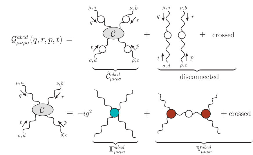
Figure 1: Upper panel: Diagrams contributing to the full four-gluon Green’s function, $\mathcal{G}^{abcd}_{\mu\nu\rho\sigma}$, separated into connected, $\mathcal{\widetilde{C}}^{abcd}_{\mu\nu\rho\sigma}$, and disconnected parts. Lower panel: Schematic decomposition of the amputated four-gluon Green’s function, $\mathcal{C}^{abcd}_{\mu\nu\rho\sigma}$, into the 1PI vertex, $-ig^{2}{\rm{I}}\!\Gamma^{abcd}_{\mu\nu\rho\sigma}$, and the 1PR terms $\mathbb{V}^{abcd}_{\mu\nu\rho\sigma}$.

In general kinematics, both ${{\rm{I}}\!\Gamma}^{abcd}_{\mu\nu\rho\sigma}$ and $\overline{{\rm{I}}\!\Gamma}^{abcd}_{\mu\nu\rho\sigma}$ possess a multitude of Lorentz and color structures, leading to a large number of form factors. In this work, we focus on the projection of the full four-gluon vertex on its tree-level structure, i.e.,

$$D_{\!\text{{4g}}}(q,r,p,t):={\mathcal{P}}(q,r,p,t)\odot\overline{\rm{I}}\!\Gamma(q,r,p,t)\,,$$ (10)

where the symbol “$\odot$” denotes the full contraction of all Lorentz and color indices, and the projector ${\mathcal{P}}$ is defined as

$${\mathcal{P}}(q,r,p,t):=\frac{\overline{\Gamma}_{0}(q,r,p,t)}{\overline{\Gamma}_{0}(q,r,p,t)\odot{\overline{\Gamma}}\vphantom{\Gamma}_{0}(q,r,p,t)}\,.$$ (11)

Evidently, for $\overline{\rm{I}}\!\Gamma^{abcd}_{\mu\nu\rho\sigma}=\overline{\Gamma}_{0\,\mu\nu\rho\sigma}^{abcd}$ we get $D_{\!\text{{4g}}}=1$. In addition, it is clear from Eqs. (10) and (11) that $D_{\!\text{{4g}}}(q,r,p,t)$ is completely Bose symmetric under the exchange of any pair of its arguments.

For the rest of this work we specialize to the case of the soft kinematics, defined by setting $t=0$ and keeping the other three momenta arbitrary but space-like, $q^{2},r^{2},p^{2}<0$. In particular, we will define the corresponding Euclidean momenta $q^{2},p^{2},r^{2}=-q^{2}_{{\scriptscriptstyle E}},-p^{2}_{{\scriptscriptstyle E}},-r^{2}_{{\scriptscriptstyle E}}>0$, and drop the subscript “E” throughout. The evaluation of the limit $t\to 0$ will be carried out “symmetrically” [89], namely

$$\lim_{t\to 0}\frac{t^{\sigma}t^{\sigma^{\prime}}}{t^{2}}=\frac{\delta^{\sigma\sigma^{\prime}}}{d}\,, \lim_{t\to 0}P^{\sigma\sigma^{\prime}}(t)=\delta^{\sigma\sigma^{\prime}}\left(1-\frac{1}{d}\right)\,,$$ (12)

where $d$ is the dimension of space-time.

Note that while the SDE determines directly ${\rm{I}}\!\Gamma^{abcd}_{\mu\nu\rho\sigma}$, the lattice computes $\mathcal{G}^{abcd}_{\mu\nu\rho\sigma}$. In order to extract ${\rm{I}}\!\Gamma^{abcd}_{\mu\nu\rho\sigma}$ on the lattice, the redundant contributions must be either eliminated by means of an appropriate choice of kinematics, or explicitly subtracted out. In particular, the disconnected contributions can be removed provided that no two momenta add up to zero, e.g., $q+r\neq 0$, and similarly for all other pairs of momenta; these conditions eliminate propagator-like transitions, due to the non-conservation of momentum. As for the 1PR term, its contribution may be subtracted out by capitalizing on the ample knowledge on the structure of the gluon propagator and three-gluon vertex [46, 58, 85, 14, 86, 87, 88]. Specifically, we combine Eqs. (6) and (10) to obtain

$$D_{\!\text{{4g}}}(q,r,p,0):=\lim_{t\to 0}\,{\mathcal{P}}\odot(\mathcal{\overline{C}}-\overline{\mathbb{V}})\,,$$ (13)

In order to subtract out $\overline{\mathbb{V}}$ we employ an excellent approximation for the three-gluon vertices contained in it. Specifically, we set [85, 14, 86, 87, 88].

$$\!\!\overline{{\rm{I}}\!\Gamma}^{\,\alpha\mu\nu}(q,r,p)=\mathit{L}_{{sg}}(s^{2})\overline{\Gamma}_{\!0}^{\,\alpha\mu\nu}(q,r,p)\,,\quad\!\!\!s^{2}=\frac{1}{2}(q^{2}+r^{2}+p^{2})\,,$$ (14)

where $\mathit{L}_{{sg}}(s^{2})$ is the form factor associated with the soft-gluon limit of the three-gluon vertex $(q=0,r=-p)$, and has been accurately determined in lattice simulations [53, 54, 90, 86, 91, 60, 58] and continuous studies [92, 93, 94, 87]. Implementing this approximation, we have that

$$\lim_{t\to 0}\,{\mathcal{P}}\odot\overline{\mathbb{V}}=f_{qrp}\,\Delta(p^{2})\,\mathit{L}_{{sg}}(p^{2})\mathit{L}_{{sg}}(s^{2})\,+\,\text{crossed}\,,$$ (15)

with

$$\!\!\!f_{qrp}\!=\!\frac{[5(q^{2}+r^{2})+p^{2}]}{{72q^{2}r^{2}}}\left[(q^{2}-r^{2}+p^{2})^{2}\!-\!4q^{2}p^{2}\right]\!\,.$$ (16)

3 SDE analysis

We next determine the form factor $D_{\!\text{{4g}}}(q,r,p,t)$ defined in Eq. (10) through appropriate projections of the SDE governing ${\rm{I}}\!\Gamma_{\mu\nu\rho\sigma}^{abcd}$. In particular, we employ the formalism of the 4PI effective action [95, 96, 97, 98, 93] at the four-loop level [99, 100]; the diagrammatic representation of the resulting SDE is given in Fig. 2. Note that the dotted lines carrying an arrow in diagram ($d_{1}$) denote the ghost propagator, $D(q^{2})=iF(q^{2})/q^{2}$, where $F(q^{2})$ is the ghost dressing function, while the dark-blue circles stand for the fully-dressed ghost-gluon vertices.

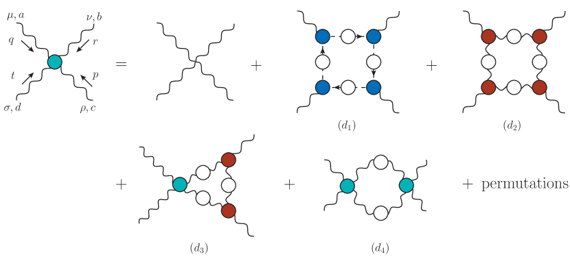
Figure 2: Diagrammatic representation of the one-loop dressed SDE for the full four-gluon vertex, ${{\rm{I}}\!\Gamma}^{abcd}_{\mu\nu\rho\sigma}$, derived from the four-loop 4PI effective action. We omit contributions obtained through permutations of the external legs.

Then, contracting both sides of the SDE by the projector ${\cal T}^{\mu^{\prime}\nu^{\prime}\rho^{\prime}\sigma^{\prime}}_{\mu\nu\rho\sigma}$ given in Eq. (5), we get [suppressing the arguments $(q,r,p,t)$]

$$\overline{{\rm{I}}\!\Gamma}^{abcd}_{\,\mu\nu\rho\sigma}=\overline{\Gamma}_{\!0\,\mu\nu\rho\sigma}^{abcd}\,+\sum_{i=1}^{4}\left(\bar{d}^{s}_{i}\right)^{abcd}_{\mu\nu\rho\sigma}\,,$$ (17)

with

$$(\bar{d}_{i}^{s})^{abcd}_{\mu\nu\rho\sigma}:={\cal T}^{\mu^{\prime}\nu^{\prime}\rho^{\prime}\sigma^{\prime}}_{\mu\nu\rho\sigma}({d}_{i})^{abcd}_{\mu^{\prime}\nu^{\prime}\rho^{\prime}\sigma^{\prime}}+\cdots\,,$$ (18)

where the ellipsis denotes the permutations corresponding to each graph (not shown in Fig. 2).

The renormalization of this SDE is implemented multiplicatively, following standard procedures. Due to the fact that all vertices in the diagrams of Fig. 2 are fully-dressed, the only renormalization constant that survives is that of the four-gluon vertex, defined through ${\rm{I}}\!\Gamma^{abcd}_{\!\!{\scriptscriptstyle R}\,\mu\nu\rho\sigma}=Z_{4}{\rm{I}}\!\Gamma^{abcd}_{\mu\nu\rho\sigma}$ [83]. In particular,

$$\overline{{\rm{I}}\!\Gamma}^{abcd}_{{\!\!R}\,\mu\nu\rho\sigma}=Z_{4}\overline{\Gamma}_{\!0\,\mu\nu\rho\sigma}^{abcd}\,+\sum_{i=1}^{4}\left(\bar{d}^{s}_{i\,{\scriptscriptstyle R}}\right)^{abcd}_{\mu\nu\rho\sigma}\,,$$ (19)

where the index “$R$” in $(\bar{d}^{s}_{i\,{\scriptscriptstyle R}})$ indicates that all ingredients comprising this set of diagrams have been replaced by their renormalized counterparts.

Note that in order to derive the expression for $D_{\!\text{{4g}}}(q,r,p,t)$ in the soft kinematics defined in the introduction, one has to act on Eq. (19) with the projector given in Eq. (11), and in the sequence take the limit $t\to 0$, with the help of Eq. (12). After doing these steps, we find that

$$D_{\!\text{{4g}}}(q,r,p,0)=Z_{4}+\lim_{t\to 0}\,\sum_{i=1}^{4}\mathcal{P}\odot\left(\bar{d}_{i}^{s}\right)(q,r,p,t)\,,$$ (20)

where we suppress the index “$R$” to avoid notational clutter.

In general kinematics, the principal variable for exploring the degree of planar degeneracy displayed by the four gluon vertex is

$$\bar{s}^{2}=\frac{1}{2}(q^{2}+r^{2}+p^{2}+t^{2})\,,$$ (21)

while the corresponding variable for the three-gluon vertex is the $s^{2}$ of Eq. (14). Evidently, in the soft configuration ($t=0$) the $\bar{s}^{2}$ of Eq. (21) reduces to the $s^{2}$ of Eq. (14).

In this limit, in addition to the $s^{2}$, it is convenient to introduce two supplementary kinematic variables, $x$ and $y$, defined by [85, 86, 87]

$$x :=\frac{\sqrt{3}(r^{2}-q^{2})}{2s^{2}}\,,\quad y:=\frac{q^{2}+r^{2}-2p^{2}}{2s^{2}}\,,$$ (22)

where, due to momentum conservation, $x$ and $y$ are constrained to the unit disk $x^{2}+y^{2}\leq 1$. Additionally, it is convenient to employ polar coordinates $(R,\phi)$ defined by

$$R=(x^{2}+y^{2})^{\!1/2}\,, \phi=\arctan(y/x)\,.$$ (23)

Hence, with this change of variables we have $D_{\!\text{{4g}}}(q,r,p,0)\to D_{\!\text{{4g}}}(s^{2}\!,R,\phi)$.

By appealing to the Bose-symmetry of the four-gluon vertex and the analysis of [88], one may show that only one sixth of this disk is relevant; the remaining five regions can be obtained by applying to $D_{\!\text{{4g}}}(s^{2}\!,R,\phi)$ simple transformations derived from Eq. (22). In the numerical analysis, we isolate one such region by restricting $\phi$ to satisfy the constraint ${\pi}/{6}\leq\phi\leq{\pi}/{2}$. In particular, we have defined a grid of configurations over this region as shown in Fig. 3. The grid is defined by taking the line with $\phi=\pi/3$, and taking points over this and parallel lines so that the result is uniformly distributed.

The approximation we employ for the $\overline{{\rm{I}}\!\Gamma}^{abcd}_{\mu\nu\rho\sigma}$ present on the rhs of Eq. (20) is analogous to the planar degeneracy relation shown in Eq. (14) for the three-gluon vertex. Namely, we take

$$\overline{{\rm{I}}\!\Gamma}_{\mu\nu\rho\sigma}^{abcd}(q,r,p,t) \approx D_{\!\text{{4g}}}^{*}(\bar{s}^{2})\overline{\Gamma}_{\!0~{}\!\!\mu\nu\rho\sigma}^{abcd}(q,r,p,t)\,,$$ (24)

where the form of $D_{\!\text{{4g}}}^{*}(\bar{s}^{2})$ will be determined through an iterative process.

By substituting Eqs. (24) and (21) in the SDE (19), $D_{\!\text{{4g}}}(s^{2}\!,R,\phi)$ reads

$$\!\!\!\!D_{\!\text{{4g}}}(s^{2}\!,R,\phi)=Z_{4}+\left[\int_{k}\!\!K_{1}+\!\!\int_{k}\!\!D_{\!\text{{4g}}}^{*}K_{2}+\!\!\int_{k}\!\!D_{\!\text{{4g}}}^{*2}K_{3}\right]\,,$$ (25)

for kernels $K_{i}$, whose form will not be specified here.

In order to determine the renormalization constant $Z_{4}$, we employ a variant of the momentum subtraction (MOM) scheme [101, 102], defined through the condition

$$D_{\!\text{{4g}}}(s^{2},R^{\,0},\phi^{\,0})\rvert_{s^{2}=\mu^{2}}=1\,,$$ (26)

where $\mu$ is the renormalization point, and the set $(R^{0},\phi^{0})$ defines a particular kinematic configuration on the disk of Fig. 3. Applying Eq. (26) on Eq. (25), we find

$$Z_{4}=1-\left[\int_{k}\!\!K_{1}+\!\!\int_{k}\!\!D_{\!\text{{4g}}}^{*}K_{2}+\!\!\int_{k}\!\!D_{\!\text{{4g}}}^{*2}K_{3}\right]_{\begin{subarray}{c}\!\!\!\!\!s^{2}\to\mu^{2}\\ R,\phi\to R^{\,0}\!\!,\phi^{\,0}\end{subarray}}\,\,\,.$$ (27)

In what follows we choose $(R^{0},\phi^{0})=(0.71,\pi/3)$, highlighted with a black circle in the central part of Fig. 3; this point lies on the aforementioned grid, and is near the center of the region. This choice is arbitrary, and we have confirmed that using different configurations for renormalization procedure only change our results by a multiplicative factor. In addition, we choose $\mu=4.3$ GeV.

For the numerical evaluation of the SDE we employ the following inputs. For the gluon propagator, $\Delta(r^{2})$, and ghost dressing function, $F(r^{2})$, we use the fits to the lattice results of [46, 58] given by Eqs. (C11) and (C6) of [25], respectively. For the transversely projected ghost-gluon vertex we use the SDE results of  [69, 14], while for the three-gluon vertices we employ Eq. (14), with $\mathit{L}_{{sg}}(r^{2})$, given by a fit to the lattice data of [60] expressed by Eq. (C12) in [25]. Both vertices have been consistently renormalized by employing Eqs. (B6) and (B7) of [83]. Finally, we use $\alpha_{s}(\mu^{2})=g^{2}/4\pi=0.27$, as obtained in Sec. 6.

The iterative process for determining $D_{\!\text{{4g}}}(s^{2}\!,R,\phi)$ may be summarized as follows:

(i) The initial input for the $D_{\!\text{{4g}}}^{*}$ on the rhs of Eq. (25) is simply its tree-level value, i.e., $D_{\!\text{{4g}}}^{*}\to 1$.

(ii) $D_{\!\text{{4g}}}(s^{2}\!,R,\phi)$ is then determined through the numerical integration of Eqs. (25) and (27). For $s^{2}$ we employ a grid distributed logarithmically over the interval $[10^{-4},10^{4}]~{}\text{GeV}^{2}$, whereas $R$ and $\phi$ are evaluated on the $N=491$ points of the grid sketched in Fig. 3.

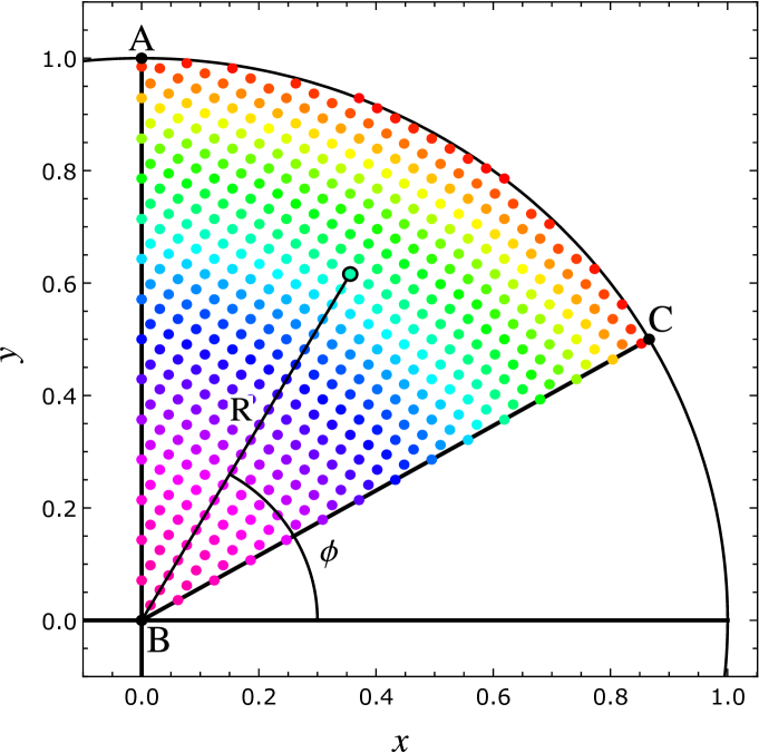
Figure 3: Representation of the 491 kinematic configurations computed on the ($x$, $y$) plane. The black points $A$ and $C$ denote the collinear configurations $(p,-p,0,0)$ and $(p,p,-2p,0)$, respectively, while $B$ is the symmetric configuration defined by $p_{1}^{2}=p_{2}^{2}=p_{3}^{2}$. We also highlight in polar coordinates $(R,\phi)$ the configuration $(R^{0},\phi^{0})=(0.71,\pi/3)$ used for renormalizing the SDE.

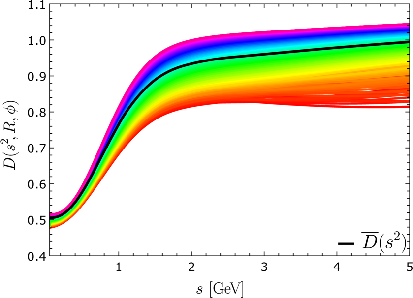
Figure 4: The form factor $D_{\!\text{{4g}}}(s^{2}\!,R_{i},\phi_{i})$ for all configurations studied, and the corresponding average $\overline{D}(s^{2})$ (black curve). Note that the color code used corresponds to that of the associated configuration in the kinematic disk in Fig. 3.

(iii) Then, we compute the simple average of these $N$ configurations by

$$\overline{D}(s^{2})=\frac{1}{N}\sum_{i=1}^{N}D_{\!\text{{4g}}}(s^{2}\!,R_{i},\phi_{i})\,,$$ (28)

which will be used as the “seed” for the next iteration. Specifically, we replace $D_{\!\text{{4g}}}^{*}\to\overline{D}$ into Eqs. (25) and (27) and re-compute $D_{\!\text{{4g}}}(s^{2}\!,R,\phi)$ for the same values of the external grid.

(iv) The iterative procedure outlined above is repeated, and at each step, the average, $\overline{D}(s^{2})$, defined in Eq. (28), is calculated. Our convergence criterion is defined when the relative error between two consecutive averages is smaller than $0.1\%$.

(v) When this is achieved, we use the last $\overline{D}(s^{2})$ as input to obtain the final results for $D_{\!\text{{4g}}}(s^{2}\!,R_{i},\phi_{i})$.

The results for both $D_{\!\text{{4g}}}(s^{2}\!,R_{i},\phi_{i})$ and $\overline{D}(s^{2})$ are shown in Fig. 4. Each configuration corresponds to a choice of $(R_{i},\phi_{i})$ and is color coded according to its position in the kinematic disk of Fig. 3, while the average is shown in black.

Notice that there is a clear pattern between the position of a configuration on the disk and its overall behavior with respect to $\overline{D}(s^{2})$: configurations closer to the center are above the average, while those closer to the edge are below it. We emphasize that the majority of the 491 curves are located very close to the total average, see Sec. 5 for details. This observation indicates the extent to which the form factor satisfies planar degeneracy, i.e.,

$$D_{\!\text{{4g}}}(s^{2}\!,R,\phi)\approx\overline{D}(s^{2})\,.$$ (29)

A detailed analysis of this relation is given in Sec. 5.

4 Vertex form factors from lattice QCD

In order to obtain lattice results for the four-gluon vertex in the soft kinematics, we have exploited 10.000 quenched lattice gauge field configurations in the Landau gauge, whose set-up parameters are (the number of configurations within parenthesis): $\beta=5.6$ (2.000), $5.7$ (1.000), $5.8$ (2.000), $6.0$ (2.000), $6.2$ (2.000), and $6.4$ (1.000) for $L/a=32$. The lattice spacings have been obtained using the absolute calibration [103] at $\beta=5.8$, and a relative calibration based on the gluon propagator scaling [57] for the rest of the $\beta$’s. For each set of momenta, we have exploited the full discrete lattice symmetry to average over all equivalent momenta with respect to permutations of Lorentz indices or signs among components. Moreover, as the lattice artifacts that break rotational symmetry (termed H4-errors) are typically far smaller than the statistical errors associated with three- or four-point correlation functions, we will average together all the sets of momenta that differ by higher-order H4 invariants [104, 105, 88].

Following the analysis of Sec.2, we use Eqs. (13) and (15) to remove from $D_{\!\text{{4g}}}(q,r,p,0)$ the 1PR contributions. The required subtraction is carried out individually for each kinematic configuration, using the available lattice data for the functions $\Delta(r^{2})$ and $\mathit{L}_{{sg}}(r^{2})$. Subsequently, the unrenormalized data sharing the same value of the Bose invariant $s^{2}$ are averaged, defining the quantity $\overline{D}_{\!\textit{{L}}}(s^{2})$.

The renormalization procedure employed on the lattice is different from that used in the SDE analysis, i.e., the MOM condition Eq. (26); however, the the two schemes coincide in the limit of exact planar degeneracy. Specifically, on the lattice the multiplicative renormalization constant, $Z_{4}$ [defined right before Eq. (19)] is fixed by imposing on the averaged data the condition

$$\overline{D}_{\!\textit{{L}}}^{{\scriptscriptstyle R}}(s^{2}) =Z_{4}\overline{D}_{\!\textit{{L}}}(s^{2})\,,\quad\overline{D}_{\!\textit{{L}}}^{{\scriptscriptstyle R}}(\mu^{2})=1\,,$$ (30)

with the renormalization point $\mu=4.3~{}\mbox{GeV}$. As was done with the SDE results, in what follows we suppress the suffix “$R$”.

Note that all lattice errors are statistical, computed through the application of the “Jack-knife method”. Moreover, the systematic errors stemming from the assumption of perfect planar degeneracy are subleading compared to the statistical; this is corroborated by the smooth behavior and small dispersion exhibited by the data for $\overline{D}_{\!\textit{{L}}}$, displayed in terms of $s^{2}$ in Fig. 5. The same is true for the errors associated with the continuum limit; therefore, the dependence on the lattice spacing $a$ has been suppressed in Eq. (30).

In order to perform a meaningful comparison with the SDE-derived average of Fig. 4, the form factor $\overline{D}(s^{2})$ is rescaled in order to match the lattice renormalization scheme of Eq. (30). This is accomplished through the operation $\overline{D}(s^{2})\to\overline{D}_{\!\textit{{N}}}(s^{2}):=\overline{D}(s^{2})/\overline{D}(\mu^{2})$, where $\overline{D}_{\!\textit{{N}}}(s^{2})$ denotes the normalized average, satisfying $\overline{D}_{\!\textit{{N}}}(\mu^{2})=1$.

In addition, we introduce a band surrounding the SDE-derived results indicating uncertainties associated with the tree-gluon form factor $\mathit{L}_{{sg}}(r^{2})$. This is implemented by repeating the iterative procedure outlined in the previous section, and solving Eq. (25) numerically using as input for $\mathit{L}_{{sg}}(r^{2})$ the band defined by Eq. (C13) in [25].

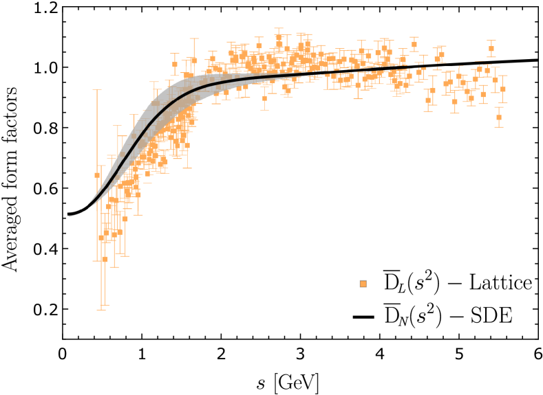
Figure 5: Comparison between the averaged form factor obtained from the lattice, $\overline{D}_{\!\textit{{L}}}(s^{2})$, and the normalized average from the SDE, $\overline{D}_{\!\textit{{N}}}(s^{2})$. The band around $\overline{D}_{\!\textit{{N}}}(s^{2})$ denotes the propagation of the statistical error associated with the three-gluon vertex.

In Fig. 5, the lattice results for $\overline{D}_{\!\textit{{L}}}(s^{2})$ are shown for all values of $\beta$, and are compared to $\overline{D}_{\!\textit{{N}}}(s^{2})$; we have a total of $N_{\rm{\scriptstyle{lat}}}=250$ points. We observe that the averaged form factors computed with both methods are quantitatively rather similar. The discrepancy between both results may be measured by the mean absolute percentage error, $\sigma$, i.e.,

$$\sigma=\frac{1}{n}\sum_{i=1}^{n}\left|\frac{\overline{D}_{\!\textit{{N}}}(s_{i}^{2})-\overline{D}_{\!\textit{{L}}}(s_{i}^{2})}{\overline{D}_{\!\textit{{L}}}(s_{i}^{2})}\right|\!\times\!100\%\,,$$ (31)

with $s_{i},\,i\!=\!1,\ldots,n$, denoting the momenta $s$ of the $n$ lattice data points within a certain interval in Fig. 5. Considering the complete data set, with $n=N_{\rm{\scriptstyle{lat}}}$, we find $\sigma=7\%$. As is evident from Fig. 5, the largest deviations between $\overline{D}_{\!\textit{{N}}}(s_{i}^{2})$ and $\overline{D}_{\!\textit{{L}}}(s_{i}^{2})$ occur for $s<1~{}\text{GeV}$, for which we find (with $n=29$) $\sigma=19\%$, and $s>4.5~{}\text{GeV}$ (with $n=20$), which yields $\sigma=8\%$.

Both results display an infrared suppression with respect to the tree-level value (unity), remaining positive for the entire range of momentum. Note that, at the origin, the SDE result reaches a finite value; in fact, one may check the finiteness by directly setting $s=0$ in Eq. (25), and taking the limit when all momenta vanish. Instead, the lattice appears inconclusive on this matter, because the data in that region come with large errors, and do not reach below $s\leq 0.5~{}\text{GeV}$. In addition, one can also see that the expected error in $\mathit{L}_{{sg}}(r^{2})$ has only a mild effect on $\overline{D}_{\!\textit{{N}}}(s^{2})$ in the region $s\in[0.4,3]~{}\text{GeV}$.

Finally, we note that SDE and lattice select their kinematic configurations differently: in contrast to the random sampling obtained in the Monte Carlo method, Fig. 3 is composed of uniformly spaced points. However, given the relatively high number of configurations probed, together with the smoothness of $D_{\!\text{{4g}}}(s^{2}\!,R,\phi)$ observed in Fig. 4, the discrepancy introduced by this difference is minimal.

5 Deviations from planar degeneracy

In this section we investigate the accuracy of the planar degeneracy, as expressed through Eq. (29), and propose an adjustment that provides a more accurate approximation for this form factor.

To accomplish this, we compute the relative percentage deviation of $D_{\!\text{{4g}}}(s^{2}\!,R_{i},\phi_{i})$ from the total average, $\overline{D}(s^{2})$, through the relative deviation

$$\delta^{i}(s^{2})\!=\!\left|\frac{D_{\!\text{{4g}}}(s^{2}\!,R_{i},\phi_{i})-\overline{D}(s^{2})}{D_{\!\text{{4g}}}(s^{2}\!,R_{i},\phi_{i})}\right|\!\times\!100\%,\quad i\!=\!1,\cdots\!,491\,.$$ (32)

For $s\leq 1~{}\text{GeV}$, we find that the maximum error $\delta^{i}(s^{2})\leq 12\%$. It is clear from Fig. 4 that as $s$ grows, the separation between curves increases; this tendency is captured by the $\delta^{i}(s^{2})$, which also increases within the range $1<s\leq 6~{}\text{GeV}$, reaching a maximum value of $22\%$. Note, however, that for the vast majority of configurations, $\delta^{i}(s^{2})$ is considerably smaller: out of the $491$ configurations analyzed, $439$ deviate from the average by less than $10\%$, while $285$ by less than $5\%$.

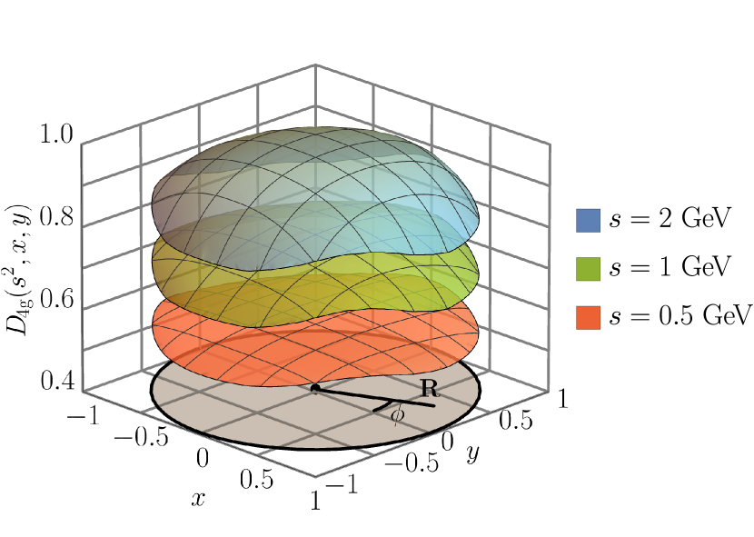
Figure 6: $D_{\!\text{{4g}}}(s^{2}\!,R,\phi)$ plotted as a function of $x$ and $y$ for selected values of $s$. The dependence on $x$ and $y$ is manifested by a deviation from perfect flatness, indicating a violation of planar degeneracy.

The property of planar degeneracy can also be appreciated directly by plotting $D_{\!\text{{4g}}}(s^{2}\!,R,\phi)$ as a function of $x$ and $y$, and analyzing the “flatness” of these surfaces for a fixed value of $s^{2}$. The result is shown in Fig. 6. There, one clearly sees that for $s=0.5$ GeV and $s=1$ GeV, the $D_{\!\text{{4g}}}(s^{2}\!,R,\phi)$ is almost perfectly constant, i.e., nearly independent of the variables $x$ and $y$.

For $s=2$ GeV, one sees a bending more pronounced at the edges of the disk represented in Fig. 3, and the appearance of a plateau in the internal region of the disk i.e., $R\lessapprox 0.5$.

An interesting feature regarding Fig. 6 is that the deviation from planar degeneracy, manifested in the curvature of the surfaces, depends almost exclusively on the radius $R$, showing minimal dependence on the angle $\phi$.

This property suggests that instead of simply using $\overline{D}(s^{2})$, a more precise approximation to $D_{\!\text{{4g}}}(s^{2}\!,R,\phi)$ may be achieved by taking in consideration both the dependence on $s^{2}$ and the radius $R$.

We explore this possibility by performing an average over the angle $\phi$. In particular, we interpolate the data points so that $\phi$ varies continuously in the interval $[\pi/6,\pi/2]$, and sample $N_{\phi}=10$ equally spaced angles $\phi^{i}$, $i=1,\ldots,N_{\phi}$. Thus, in analogy to Eq. (28), we define

$$\overline{D}(s^{2},R)=\frac{1}{N_{\phi}}\sum_{i}^{N_{\phi}}D_{\!\text{{4g}}}(s^{2},R,\phi^{i})\,.$$ (33)

Then, the improvement achieved when using Eq. (33) can be appreciated by defining the relative deviation

$$\!\!\!\!\overline{\delta}^{\,i}(s^{2})\!=\!\left|\frac{D_{\!\text{{4g}}}(s^{2}\!,R_{i},\phi_{i})\!-\!\overline{D}(s^{2},R_{i})}{D_{\!\text{{4g}}}(s^{2}\!,R_{i},\phi_{i})}\right|\!\times\!100\%,~{}~{}i\!=\!1,\cdots\!,491\,.$$ (34)

In contrast to $\delta^{i}(s^{2})$, the relative error $\overline{\delta}^{\,i}(s^{2})$ has a maximum deviation of only $7\%$ over the entire range $0<s\leq 6~{}\text{GeV}$. Indeed, when compared to $D_{\!\text{{4g}}}$, with its complete momentum dependence taken into account, $\overline{D}(s^{2},R)$ offers a significant increase in accuracy over $\overline{D}(s^{2})$.

6 Effective charge

In this section we use the SDE and lattice results of Fig. 5 to construct an RGI effective charge, denoted by $\alpha_{4g}(s^{2})$. Specifically, following a standard definition [107, 26, 24, 83], we have

$$\alpha_{4g}(s^{2})=\alpha_{s}(\mu^{2})\overline{D}(s^{2})\mathcal{Z}^{2}(s^{2})\,,$$ (35)

where $\overline{D}(s^{2})$ stands for the averaged form factors shown in Fig. 5, and $\mathcal{Z}(p^{2})=p^{2}\Delta(p^{2})$ is the gluon dressing function.

Capitalizing on the RG invariance of $\alpha_{4g}(s^{2})$, the SDE approach employs the average of Fig. 4 without the normalization factor introduced in the previous section. The value $\alpha_{s}(\mu^{2})=0.27$ quoted in Sec. 3 is obtained by minimizing the discrepancy of the SDE-lattice comparison in the vicinity of the renormalization point $\mu=4.3~{}\text{GeV}$; specifically this value produces the best match in the interval $s\in[4,4.5]~{}\text{GeV}$.

The lattice determination of $\alpha_{4g}(s^{2})$ follows the same procedure described in [88], except that in Eq. (35) the implicit continuum limit $a\to 0$ has again been dropped because any non-singular, remaining dependence on the lattice spacing is hidden in the statistical noise.

Both determinations of $\alpha_{4g}(s^{2})$ are shown in Fig. 7, displaying an excellent agreement over the entire range of momenta: the mean absolute percentage error, defined in analogy to Eq. (31), is of $9\%$ for the entire interval. Let us finally stress the qualitative similarities with the result of [83], where the four-gluon form factor in Eq. (35) is evaluated in a collinear kinematic configuration.

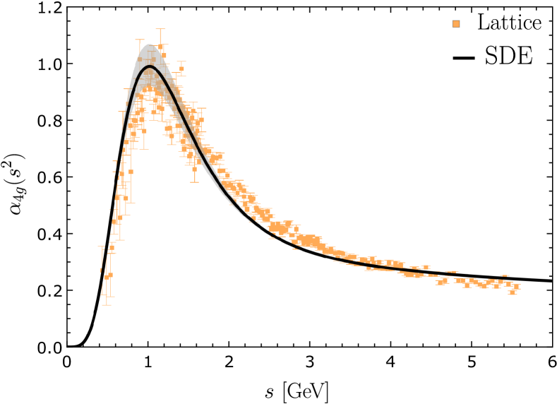
Figure 7: Lattice and SDE determinations of the $\alpha_{4g}(s^{2})$ defined by Eq. (35), with error bands associated to the statistical error of the three-gluon vertex.

7 Conclusions

In this work we have explored the nonperturbative four-gluon vertex in soft kinematics, by combining an SDE analysis and a lattice simulation, in the Landau gauge. The quantity considered is the projection of the four-gluon vertex on its tree-level tensor, averaged over a large selection of kinematic configurations sharing the same $s^{2}$.

The key hypothesis employed by both methods is the property of planar degeneracy: its use simplifies the SDE analysis, and allows for the emergence of a clear lattice signal. The results of both approaches are in very good agreement, affirming the overall robustness of the underlying picture.

Importantly, a further analysis of the SDE results establishes that planar degeneracy is only approximate, as already argued in [83]. Here, we have indicated how deviations of this property can be accurately taken into account, suggesting an improved description for this vertex in future applications.

We emphasize that, while the quantity $D_{\!\text{{4g}}}(q,r,p,t)$ considered in this work is expected to be dominated by the classical form factor, in a future analysis this assumption may be explicitly tested, by formally eliminating unwanted admixtures through suitable projections, in the spirit of [83].

We finally point out that, in the limit of exact planar degeneracy, the effective charge $\alpha_{4g}(s^{2})$ would measure, in a configuration-independent way, the strength of the four-gluon interaction. Even though the observed deviations from the planar degeneracy invalidate this possibility, their reduced size makes $\alpha_{4g}(s^{2})$ a rather useful instrument for describing the underlying dynamics.

References

- Yang and Mills [1954] C.-N. Yang, R. L. Mills, Phys. Rev. 96 (1954) 191–195.
- Gross and Wilczek [1973] D. J. Gross, F. Wilczek, Phys. Rev. Lett. 30 (1973) 1343–1346.
- Politzer [1973] H. D. Politzer, Phys. Rev. Lett. 30 (1973) 1346–1349.
- Marciano and Pagels [1978] W. J. Marciano, H. Pagels, Phys. Rept. 36 (1978) 137.
- Roberts and Williams [1994] C. D. Roberts, A. G. Williams, Prog. Part. Nucl. Phys. 33 (1994) 477–575.
- Alkofer and von Smekal [2001] R. Alkofer, L. von Smekal, Phys. Rept. 353 (2001) 281.
- Fischer [2006] C. S. Fischer, J. Phys. G 32 (2006) R253–R291.
- Binosi and Papavassiliou [2009] D. Binosi, J. Papavassiliou, Phys. Rept. 479 (2009) 1–152.
- Cloet and Roberts [2014] I. C. Cloet, C. D. Roberts, Prog. Part. Nucl. Phys. 77 (2014) 1–69.
- Aguilar et al. [2016] A. C. Aguilar, D. Binosi, J. Papavassiliou, Front. Phys.(Beijing) 11 (2016) 111203.
- Eichmann et al. [2016] G. Eichmann, H. Sanchis-Alepuz, R. Williams, R. Alkofer, C. S. Fischer, Prog. Part. Nucl. Phys. 91 (2016) 1–100.
- Huber [2020] M. Q. Huber, Phys. Rept. 879 (2020) 1–92.
- Papavassiliou [2022] J. Papavassiliou, Chin. Phys. C 46 (2022) 112001.
- Ferreira and Papavassiliou [2023] M. N. Ferreira, J. Papavassiliou, Particles 6 (2023) 312–363.
- Roberts [2008] C. D. Roberts, Prog. Part. Nucl. Phys. 61 (2008) 50–65.
- Aguilar et al. [2008] A. C. Aguilar, D. Binosi, J. Papavassiliou, Phys. Rev. D78 (2008) 025010.
- Boucaud et al. [2008] P. Boucaud, J. Leroy, L. Y. A., J. Micheli, O. Pène, J. Rodríguez-Quintero, J. High Energy Phys. 06 (2008) 099.
- Eichmann et al. [2010] G. Eichmann, R. Alkofer, A. Krassnigg, D. Nicmorus, Phys. Rev. Lett. 104 (2010) 201601.
- Fischer et al. [2009] C. S. Fischer, A. Maas, J. M. Pawlowski, Annals Phys. 324 (2009) 2408–2437.
- Rodriguez-Quintero [2011] J. Rodriguez-Quintero, J. High Energy Phys. 01 (2011) 105.
- Huber et al. [2012] M. Q. Huber, A. Maas, L. von Smekal, J. High Energy Phys. 11 (2012) 035.
- Gao et al. [2021] F. Gao, J. Papavassiliou, J. M. Pawlowski, Phys. Rev. D 103 (2021) 094013.
- Huber [2016] M. Q. Huber, Phys. Rev. D 93 (2016) 085033.
- Huber [2020] M. Q. Huber, Phys. Rev. D 101 (2020) 114009.
- Aguilar et al. [2022] A. C. Aguilar, M. N. Ferreira, J. Papavassiliou, Phys. Rev. D 105 (2022) 014030.
- Cyrol et al. [2015] A. K. Cyrol, M. Q. Huber, L. von Smekal, Eur. Phys. J. C75 (2015) 102.
- Braun et al. [2010] J. Braun, H. Gies, J. M. Pawlowski, Phys. Lett. B684 (2010) 262–267.
- Fister and Pawlowski [2013] L. Fister, J. M. Pawlowski, Phys. Rev. D88 (2013) 045010.
- Pawlowski et al. [2004] J. M. Pawlowski, D. F. Litim, S. Nedelko, L. von Smekal, Phys. Rev. Lett. 93 (2004) 152002.
- Pawlowski [2007] J. M. Pawlowski, Annals Phys. 322 (2007) 2831–2915.
- Cyrol et al. [2018a] A. K. Cyrol, M. Mitter, J. M. Pawlowski, N. Strodthoff, Phys. Rev. D97 (2018a) 054006.
- Cyrol et al. [2018b] A. K. Cyrol, J. M. Pawlowski, A. Rothkopf, N. Wink, SciPost Phys. 5 (2018b) 065.
- Corell et al. [2018] L. Corell, A. K. Cyrol, M. Mitter, J. M. Pawlowski, N. Strodthoff, SciPost Phys. 5 (2018) 066.
- Blaizot et al. [2021] J.-P. Blaizot, J. M. Pawlowski, U. Reinosa, Annals Phys. 431 (2021) 168549.
- Horak et al. [2021] J. Horak, J. Papavassiliou, J. M. Pawlowski, N. Wink, Phys. Rev. D 104 (2021) 074017.
- Pawlowski et al. [2023] J. M. Pawlowski, C. S. Schneider, J. Turnwald, J. M. Urban, N. Wink, Phys. Rev. D 108 (2023) 076018.
- Tissier and Wschebor [2010] M. Tissier, N. Wschebor, Phys. Rev. D 82 (2010) 101701.
- Dudal et al. [2008] D. Dudal, J. A. Gracey, S. P. Sorella, N. Vandersickel, H. Verschelde, Phys. Rev. D78 (2008) 065047.
- Mintz et al. [2018] B. W. Mintz, L. F. Palhares, S. P. Sorella, A. D. Pereira, Phys. Rev. D97 (2018) 034020.
- Barrios et al. [2020] N. Barrios, M. Peláez, U. Reinosa, N. Wschebor, Phys. Rev. D 102 (2020) 114016.
- Peláez et al. [2021] M. Peláez, U. Reinosa, J. Serreau, M. Tissier, N. Wschebor, Rept. Prog. Phys. 84 (2021) 124202.
- Barrios et al. [2024] N. Barrios, P. De Fabritiis, M. Peláez, Phys. Rev. D 109 (2024) L091502.
- Cucchieri et al. [2006] A. Cucchieri, A. Maas, T. Mendes, Phys. Rev. D74 (2006) 014503.
- Cucchieri and Mendes [2007] A. Cucchieri, T. Mendes, PoS LATTICE2007 (2007) 297.
- Bogolubsky et al. [2007] I. Bogolubsky, E. Ilgenfritz, M. Muller-Preussker, A. Sternbeck, PoS LATTICE2007 (2007) 290.
- Bogolubsky et al. [2009] I. Bogolubsky, E. Ilgenfritz, M. Muller-Preussker, A. Sternbeck, Phys. Lett. B676 (2009) 69–73.
- Cucchieri et al. [2008] A. Cucchieri, A. Maas, T. Mendes, Phys. Rev. D77 (2008) 094510.
- Cucchieri and Mendes [2010] A. Cucchieri, T. Mendes, Phys. Rev. D81 (2010) 016005.
- Oliveira and Silva [2009] O. Oliveira, P. Silva, PoS LAT2009 (2009) 226.
- Oliveira and Bicudo [2011] O. Oliveira, P. Bicudo, J. Phys. G G38 (2011) 045003.
- Ayala et al. [2012] A. Ayala, A. Bashir, D. Binosi, M. Cristoforetti, J. Rodriguez-Quintero, Phys. Rev. D86 (2012) 074512.
- Oliveira and Silva [2012] O. Oliveira, P. J. Silva, Phys. Rev. D86 (2012) 114513.
- Athenodorou et al. [2016] A. Athenodorou, D. Binosi, P. Boucaud, F. De Soto, J. Papavassiliou, J. Rodriguez-Quintero, S. Zafeiropoulos, Phys. Lett. B761 (2016) 444–449.
- Duarte et al. [2016] A. G. Duarte, O. Oliveira, P. J. Silva, Phys. Rev. D94 (2016) 074502.
- Sternbeck et al. [2017] A. Sternbeck, P.-H. Balduf, A. Kizilersu, O. Oliveira, P. J. Silva, J.-I. Skullerud, A. G. Williams, PoS LATTICE2016 (2017) 349.
- Boucaud et al. [2017] P. Boucaud, F. De Soto, J. Rodriguez-Quintero, S. Zafeiropoulos, Phys. Rev. D 96 (2017) 098501.
- Boucaud et al. [2018] P. Boucaud, F. De Soto, K. Raya, J. Rodriguez-Quintero, S. Zafeiropoulos, Phys. Rev. D98 (2018) 114515.
- Aguilar et al. [2021] A. C. Aguilar, C. O. Ambrósio, F. De Soto, M. N. Ferreira, B. M. Oliveira, J. Papavassiliou, J. Rodríguez-Quintero, Phys. Rev. D 104 (2021) 054028.
- Maas [2013] A. Maas, Phys. Rept. 524 (2013) 203–300.
- Aguilar et al. [2021] A. C. Aguilar, F. De Soto, M. N. Ferreira, J. Papavassiliou, J. Rodríguez-Quintero, Phys. Lett. B 818 (2021) 136352.
- Meyer and Swanson [2015] C. A. Meyer, E. S. Swanson, Prog. Part. Nucl. Phys. 82 (2015) 21–58.
- Souza et al. [2020] E. V. Souza, M. N. Ferreira, A. C. Aguilar, J. Papavassiliou, C. D. Roberts, S.-S. Xu, Eur. Phys. J. A 56 (2020) 25.
- Huber et al. [2024] M. Q. Huber, C. S. Fischer, H. Sanchis-Alepuz, Nuovo Cim. C 47 (2024) 184.
- Eichmann et al. [2020] G. Eichmann, C. S. Fischer, W. Heupel, N. Santowsky, P. C. Wallbott, Few Body Syst. 61 (2020) 38.
- Cornwall [1982] J. M. Cornwall, Phys. Rev. D 26 (1982) 1453.
- Fischer and Alkofer [2003] C. S. Fischer, R. Alkofer, Phys. Rev. D67 (2003) 094020.
- Cui et al. [2020] Z.-F. Cui, J.-L. Zhang, D. Binosi, F. de Soto, C. Mezrag, J. Papavassiliou, C. D. Roberts, J. Rodríguez-Quintero, J. Segovia, S. Zafeiropoulos, Chin. Phys. C 44 (2020) 083102.
- Binosi et al. [2015] D. Binosi, L. Chang, J. Papavassiliou, C. D. Roberts, Phys. Lett. B742 (2015) 183–188.
- Aguilar et al. [2023] A. C. Aguilar, F. De Soto, M. N. Ferreira, J. Papavassiliou, F. Pinto-Gómez, C. D. Roberts, J. Rodríguez-Quintero, Phys. Lett. B 841 (2023) 137906.
- Boucaud et al. [2012] P. Boucaud, J. P. Leroy, A. L. Yaouanc, J. Micheli, O. Pene, J. Rodriguez-Quintero, Few Body Syst. 53 (2012) 387–436.
- Aguilar and Papavassiliou [2011] A. C. Aguilar, J. Papavassiliou, Phys. Rev. D83 (2011) 014013.
- Kondo et al. [2015] K.-I. Kondo, S. Kato, A. Shibata, T. Shinohara, Phys. Rept. 579 (2015) 1–226.
- Greensite [2003] J. Greensite, Prog. Part. Nucl. Phys. 51 (2003) 1.
- Pascual and Tarrach [1980] P. Pascual, R. Tarrach, Nucl. Phys. B 174 (1980) 123. [Erratum: Nucl.Phys.B 181, 546 (1981)].
- Brandt and Frenkel [1986] F. T. Brandt, J. Frenkel, Phys. Rev. D 33 (1986) 464.
- Papavassiliou [1993] J. Papavassiliou, Phys. Rev. D 47 (1993) 4728–4738.
- Hashimoto et al. [1994] S. Hashimoto, J. Kodaira, Y. Yasui, K. Sasaki, Phys. Rev. D 50 (1994) 7066–7076.
- Gracey [2014] J. A. Gracey, Phys. Rev. D90 (2014) 025011.
- Gracey [2017] J. A. Gracey, Phys. Rev. D 95 (2017) 065013.
- Ahmadiniaz and Schubert [2013] N. Ahmadiniaz, C. Schubert, PoS QCD-TNT-III (2013) 002.
- Ahmadiniaz and Schubert [2016] N. Ahmadiniaz, C. Schubert, Int. J. Mod. Phys. E 25 (2016) 1642004.
- Binosi et al. [2014] D. Binosi, D. Ibañez, J. Papavassiliou, J. High Energy Phys. 09 (2014) 059.
- Aguilar et al. [2024] A. C. Aguilar, M. N. Ferreira, J. Papavassiliou, L. R. Santos, Eur. Phys. J. C 84 (2024) 676.
- Colaço et al. [2024] M. Colaço, O. Oliveira, P. J. Silva, Phys. Rev. D 109 (2024) 074502.
- Eichmann et al. [2014] G. Eichmann, R. Williams, R. Alkofer, M. Vujinovic, Phys. Rev. D89 (2014) 105014.
- Pinto-Gómez et al. [2023] F. Pinto-Gómez, F. De Soto, M. N. Ferreira, J. Papavassiliou, J. Rodríguez-Quintero, Phys. Lett. B 838 (2023) 137737.
- Aguilar et al. [2023] A. C. Aguilar, M. N. Ferreira, J. Papavassiliou, L. R. Santos, Eur. Phys. J. C 83 (2023) 549.
- Pinto-Gómez et al. [2024] F. Pinto-Gómez, F. De Soto, J. Rodríguez-Quintero, Phys. Rev. D 110 (2024) 014005.
- Peskin and Schroeder [1995] M. E. Peskin, D. V. Schroeder, An introduction to quantum field theory, Advanced book program, Westview Press Reading (Mass.), Boulder (Colo.), 1995. Autre tirage : 1997.
- Boucaud et al. [2017] P. Boucaud, F. De Soto, J. Rodríguez-Quintero, S. Zafeiropoulos, Phys. Rev. D95 (2017) 114503.
- Aguilar et al. [2020] A. C. Aguilar, F. De Soto, M. N. Ferreira, J. Papavassiliou, J. Rodríguez-Quintero, S. Zafeiropoulos, Eur. Phys. J. C80 (2020) 154.
- Blum et al. [2014] A. Blum, M. Q. Huber, M. Mitter, L. von Smekal, Phys. Rev. D89 (2014) 061703.
- Williams et al. [2016] R. Williams, C. S. Fischer, W. Heupel, Phys. Rev. D93 (2016) 034026.
- Aguilar et al. [2019] A. C. Aguilar, M. N. Ferreira, C. T. Figueiredo, J. Papavassiliou, Phys. Rev. D99 (2019) 094010.
- Cornwall et al. [1974] J. M. Cornwall, R. Jackiw, E. Tomboulis, Phys. Rev. D 10 (1974) 2428–2445.
- Cornwall and Norton [1973] J. Cornwall, R. Norton, Phys. Rev. D 8 (1973) 3338–3346.
- Berges [2004] J. Berges, Phys. Rev. D 70 (2004) 105010.
- York et al. [2012] M. C. A. York, G. D. Moore, M. Tassler, JHEP 06 (2012) 077.
- Carrington and Guo [2011] M. E. Carrington, Y. Guo, Phys. Rev. D 83 (2011) 016006.
- Carrington et al. [2013] M. E. Carrington, W. Fu, T. Fugleberg, D. Pickering, I. Russell, Phys. Rev. D 88 (2013) 085024.
- Boucaud et al. [2009] P. Boucaud, F. De Soto, J. Leroy, A. Le Yaouanc, J. Micheli, et al., Phys. Rev. D79 (2009) 014508.
- Boucaud et al. [2011] P. Boucaud, D. Dudal, J. Leroy, O. Pene, J. Rodriguez-Quintero, J. High Energy Phys. 12 (2011) 018.
- Necco and Sommer [2002] S. Necco, R. Sommer, Nucl. Phys. B 622 (2002) 328–346.
- de Soto and Roiesnel [2007] F. de Soto, C. Roiesnel, J. High Energy Phys. 09 (2007) 007.
- de Soto [2022] F. de Soto, JHEP 10 (2022) 069.
- Eichmann et al. [2015] G. Eichmann, C. S. Fischer, W. Heupel, Phys. Rev. D92 (2015) 056006.
- Kellermann and Fischer [2008] C. Kellermann, C. S. Fischer, Phys. Rev. D78 (2008) 025015.