Thermal Stoner-Wohlfarth Model for Magnetodynamics of Single Domain Nanoparticles: Implementation and Validation

Abstract

We present the thermal Stoner-Wohlfarth (tSW) model and apply it in the context of Molecular Dynamics simulations. The model is validated against an ensemble of immobilized, non-interacting, randomly oriented uniaxial particles (solid superparamagnet) and a classical dilute (non-interacting) ferrofluid for different combinations of anisotropy strength and magnetic field/moment coupling, at a fixed temperature. We compare analytical and simulation results to quantify the viability of the tSW model in reproducing the equilibrium and dynamic properties of magnetic soft matter systems. We show that if the anisotropy of a particle is more than four-five times higher than the thermal fluctuations, tSW is applicable and efficient. It provides a valuable insight into the interplay between internal magnetization degrees of freedom and Browninan rotation that is often neglected in the fixed point-dipole representation-based magnetic soft matter theoretical investigations.

I Introduction

The idea to control materials using magnetic fields, inspired in the early 20th century by the works of Langevin [1, 2] and through pioneering works on magnetic fluids by Elmore [3] and later by Resler and Rosenzweig [4], has since manifested a branch of science studying magnetic soft matter. The fundamental insight from these pioneering works is that small ferromagnetic particles suspended in a magneto-passive liquid represented a paramagnetic system whose magnetisation can be described with a Langevin function. In other words, one understood that it is possible to engineer and appropriate the magnetic response of complex systems from the collective magnetic response of constituent nanoparticles that themselves have well defined and finely controllable magnetic properties. Under the umbrella term of magnetic soft matter, various magnetoresponsive systems have been explored, including ferrofluids,[5, 6, 7, 8] ferrogels,[9, 10] elastomers,[11, 12, 13, 14, 15] magnetic gels [16, 9, 17] and magnetic filaments (MFs) [18, 19], with a research action focused on generating a macroscopic response by coupling the magnetic response of magnetic nanoparticles, that can be affected via magnetic fields in a contained and precise manner, mechanically or chemically to its environment, such as a polymeric matrix or a viscous environment in general. This class of problem lends itself particularly for classical simulation studies such as Molecular Dynamics (MD). The key that unlocked such simulation studies of composite, complex magnetoresponsive systems, their magnetic properties and response to magnetic fields, is the fixed point dipole representation [20]. In this picture, the dipole moment is depicted as vector that is always coaligned with the anisotropy axis of the nanoparticle, with a fixed magnitude and orientation in the particle reference frame. The fixed point dipole representation of magnetic colloids in general is at the heart of the overwhelming majority of theoretical and classical simulation studies of magnetic fluids and magnetic soft matter [21, 22, 23, 24, 25]. It is a powerful and flexible representation, that albeit undoubtedly practical, incurs important assumptions and approximations. There are no degrees of freedom for the dipole moment to exploit with respect to the anisotropy axis. In other words, magnetic relaxation can only manifest through physical rotation of the nanoparticle body, commonly refereed to as Brownian relaxation. Strictly speaking, the fixed point dipole representation is appropriate for single-domain nanoparticles with infinitely high uniaxial anisotropy [26]. If one is only interested in applied field coupling and far field interactions, more complex magnetic colloids can also be represented as fixed point dipoles, as long as they can be considered as ideally ferro-/ferrimagnetic [27]. Clearly, the fixed point dipole representation fundamentally limits the scope of the studies based on it. In general, depending on the colloids size and/or material, it can neither be taken as given that the dipole moment is coaligned with the anisotropy axis, nor that it has a fixed orientation with respect to it. In fact, the dipole moment has degrees of freedom within the nanoparticle body, which manifest as additional magnetic relaxation mechanisms, most prominent of which is commonly refereed to as Néel relaxation. Generally, the dipole moment states within a nanoparticle correspond to local free energy minima. With Néel relaxation one implies that thermal fluctuations can cause jumps between the available states. In other words, the dipole moment can, driven by thermal fluctuations, flip its orientation with respect to the easy axis. In this context, the anisotropy energy can be interpreted as an energy barrier that needs to be surmounted in order for such a flip to occur. The Brownian and Néel relaxation are two major mechanisms in the description of the magnetic properties of single-domain nanoparticles, and are well captured with a combination of the ideas presented in the seminal works of Stoner and Wohlfarth [28], Néel [29] and Brown [30]. When modeling the dynamics of magnetic soft matter, capturing Brownian and Néel relaxation is fundamentally important [31, 32, 33, 34, 35, 36]. Beyond the academic interest in accurately describing the dynamics of magnetic nanoparticles, understanding magnetic relaxation opens numerous avenues for technological applications [37, 38, 39, 40, 41, 42, 43]. Among others, the interplay between different relaxation mechanisms is key for optimizing magnetic hyperthermia [44, 45, 46, 47].

In this work, we present the thermal Stoner-Wohlfarth (tSW) model as a low computational cost method that allows one to include explicit and accurate magnetodynamics into simulation studies of magnetic soft matter with single domain, uniaxial nanoparticles. In this context, magnetodynamics entails the Brownian and Néel relaxation mechanisms, and the ability of a dipole moment not to be co-aligned with the nanoparticle anisotropy axis in the presence of magnetic and/or dipole fields. We first introduce a formal problem description in Section I, with a detailed discussion on the relevant energy (I.1) and timescales (I.2). In Section II, the model is validated against: (a) an ensemble of immobilized, non-interacting, randomly oriented uniaxial particles (solid superparamagnet) and (b) a classical dilute (non-interacting) ferrofluid. This is equivalent to making the distinction on the basis of whether the nanoparticles exhibit only Néel relaxation mechanisms or both Brownian and Néel relaxation mechanisms, respectively. In both cases, we compare analytical and simulation results to quantify the viability of the thermal SW model in reproducing equilibrium (magnetisation; II.1) and dynamic (susceptibility; II.2) properties of magnetic soft matter systems. A detailed account of the tSW model implementation, simulation details and units is presented in Section I.3. It is important to note that the ideas behind the tSW model have been discussed and used previously [48, 49]. However, a systematic study of its applicability with respect to anisotropy energy/temperature and magnetic field strength has remained unclear up to now. Moreover, the viability and applicability of the model in the context of MD simulations of magnetic soft matter has not been explored so far.

I.1 Formal problem description

A magnetic nanoparticle is subjected to a uniform magnetic field $\vec{H}$ at a fixed temperature $T$. The classical, athermal formulation of the total magnetic energy of a nanoparticle was introduced in Stoner and Wohlfarth [28]

$$U=-\mu_{0}\mu(\vec{e}\cdot\vec{H})-KV(\vec{e}\cdot\vec{n})^{2},$$ (1)

where:

• $\mu_{0}$ is the vacuum magnetic permeability;

• $\vec{e}=\vec{\mu}/\mu=(\cos\phi\sin\theta,\sin\phi\sin\theta,\cos\theta)$ is the unit vector of the magnetic moment $\vec{\mu}$, where $\mu=|\vec{\mu}|=M_{s}V$, $\theta$ is the angle between the magnetic moment and the field and $\phi$ is the corresponding polar angle, for notations see Fig. 1;

• $M_{s}$ is the saturation magnetization of the particle material;

• $V=(\pi/6)d^{3}$ is the particle volume, $d$ is the particle diameter;

• $K$ is the particle anisotropy constant;

• $\vec{n}=(\cos\zeta\sin\psi,\sin\zeta\sin\psi,\cos\psi)$ is the unit vector of the anisotropy axis, where $\psi$ is the angle between the applied field and the anisotropy axis and $\zeta$ is the corresponding polar angle, see Fig. 1.

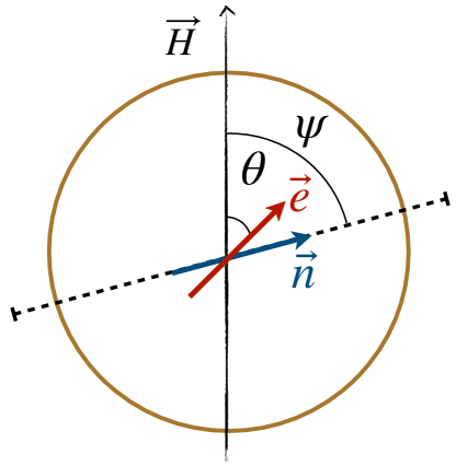
Figure 1: Geometric details including angles used in the formulation of the total magnetic energy in the Stoner-Wohlfarth model.

The problem has three characteristic energy scales: the Zeeman energy, $\mu_{0}\mu H$, the anisotropy energy, $KV$, and thermal energy, $k_{B}T$. The interplay between the characteristic energy scales is described in terms of two dimensionless parameters, namely the Langevin parameter:

$$\xi=\frac{\mu_{0}\mu H}{k_{B}T},$$ (2)

and the anisotropy parameter:

$$\sigma=\frac{KV}{k_{B}T}.$$ (3)

Additionally, the interplay between anisotropy and external field is traditionally described with the dimensionless field:

$$h=\frac{\xi}{2\sigma}=\frac{\mu_{0}M_{s}H}{2K}=\frac{H}{H_{ani}}$$ (4)

where $H_{ani}=2K/\mu_{0}M_{s}$ is the anisotropy field. For the geometry sketched in Fig. 1, Eq. 1 can be rewritten as:

$$\frac{U}{KV}=-\left(\cos(\phi-\zeta)\sin\theta\sin\psi+\cos\theta\cos\psi\right)^{2}-2h\cos\theta.$$ (5)

where, according to Stoner and Wohlfarth [28], global minima of the potential always lie in the plane spanned by $\vec{H}$ and $\vec{n}$ ($\phi=\zeta$). Eq. 5 has two minima below the critical field strength:

$$h_{cr}(\psi)=(\sin^{2/3}\psi+\cos^{2/3}\psi)^{-3/2}.$$ (6)

Above the critical field, only one global minimum remains. The particle dipole moment follows the position of the local energy minimum and instantaneously changes its direction depending on strength of $h$ in relation to $h_{cr}$. Transitions between the energy minima are not possible below $h_{cr}$ (at $T=0$). A visualisation of the energy landscape defined with Eq. 5 ($\phi=\zeta$), along with its dependence on $\theta$,$\psi$ and $h$, is provided in Fig.2. The simplest thermal formulation of the total magnetic energy would include the Néel relaxation mechanism, understood as the internal relaxation achieved through thermal fluctuation induced transitions of the dipole moment between the local energy minima in the total magnetic energy of a particle. This intuitive notion of the Néel mechanism inheres several important approximations, discussed at length below. Brownian relaxation instead refers to rotational diffusion of the particle body.

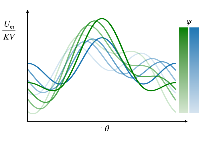
Figure 2: Visualisation of the energy (density) landscape in the Stoner-Wohlfarth model, as a function of $\theta$. Lines with a different colour saturation correspond to energy densities for a different $\psi$. The more saturated a colour appears, the more aligned the anisotropy axis is with the applied field (smaller $\psi$). Different colours correspond to different applied field strengths, where green energy density profiles correspond to a higher applied field strength then blue energy density profiles.)

I.2 Relevant time scales

Here, we discuss the timescales of the relaxation mechanisms characteristic for ensembles of magnetic nanoparticles, starting with the ones associated with internal degrees of freedom. In the absence of thermal fluctuations and an applied field, the main time scale that characterizes the magnetization relaxation in immobilized ensembles, is the damping time of the Larmor precession. From the standard Landau-Lifshitz-Gilbert (LLG) equation, it can be estimated as [50]:

$$\tau_{0}=\frac{1}{\alpha\omega_{L}}=\frac{(1+\alpha^{2})M_{s}}{2\alpha\gamma K},$$ (7)

where $\omega_{L}=\gamma\mu_{0}H_{ani}/(1+\alpha^{2})$ is the precession frequency (in the absence of an applied field), $\alpha$ is the phenomenological damping parameter with typical values in the range between 0.01 and 0.1, $\gamma\simeq 1.76\times 10^{11}~{}\textrm{s}^{-1}\textrm{T}^{-1}$ is the gyromagnetic ratio.

At any non-zero temperature, the magnetic moment is subjected to thermal fluctuations. The characteristic time scale of its rotational diffusion in the limit of weak field and weak anisotropy (i.e., at $\xi\ll 1$ and $\sigma\ll 1$) is given by

$$\tau_{D}=\frac{(1+\alpha^{2})\mu}{2\alpha\gamma k_{B}T}=\sigma\tau_{0}.$$ (8)

The time scale $\tau_{D}$ (sometimes referred to as the Debye time) arises naturally, as thermal noise is introduced into the LLG equation and it is required to reproduce the Gibbs-Boltzmann distribution in thermodynamic equilibrium [51].

However, for nanoparticles with $\sigma\geq 1$, it is common to distinguish two mechanisms – 1) jumps between energy minima and 2) fast fluctuations in the vicinity of a given minimum [52, 26]. In Raikher and Stepanov [52] terminology, these are called “interwell” and “intrawell” relaxation processes, respectively. For sufficiently large anisotropies, $\sigma\gg 1$, one might neglect the intrawell processes entirely. In this approximation, magnetic moments are always in one of the local minima and are only allowed to jump between them. L. Néel in 1949 was the first to use this approximation and suggest that the magnetization relaxation time due to over-barrier thermal jumps follows an Arrhenius-like law [29]. In 1963, the Néel result was improved by W.F. Brown Jr. [30]. With the help of the Kramers escape rate theory, Brown gave the following high-barrier approximation for the magnetization relaxation time (the so-called Néel time):

$$~{}\tau_{N}(\sigma\gg 1)=\frac{\tau_{D}}{2\sigma}\sqrt{\frac{\pi}{\sigma}}\exp\sigma.$$ (9)

Formally, the Néel time $\tau_{N}$ is the inverse of the smallest non-vanishing eigenvalue of the Fokker-Planck equation, that Brown formulated on the basis of the stochastic Landau-Lifshitz-Gilbert equation. Eq. 9 is only valid for uniaxial particles in zero field. However, in the literature one can find multiple approximations for $\tau_{N}$ in static fields of different orientations, as well as for other anisotropy types [26, 53]. Brown in his work also demonstrated that the zero-field rate of over-barrier jumps is not affected by the Larmor precession and that corresponding term in the Fokker-Planck equation can be safely omitted as one is looking for $\tau_{N}$. The same is true, if the field is applied parallel to the easy axis ($\psi=0$). This is a general property of the Fokker-Plank-Brown equation for problems that possess axial symmetry. However, for all other cases ($\psi\neq 0$ or different anisotropy types), precession will affect magnetic relaxation and should in principle be explicitly taken into consideration [54, 55]. Omitting precession in the general case limits the results to the field frequencies below the ferromagentic resonance range.

Finally, we introduce the timescales of relaxation mechanisms associated with external degrees of freedom in nanoparticles. If the particle is suspended in a viscous medium, two more relaxation times, connected to its mechanical rotation, must be introduced [56]. If a particle is coated with a non-magnetic shell of width $l$, its hydrodynamic diameter can be calculated as $d_{H}=d+2l$. The inertial decay time is:

$$\tau_{J}=\frac{J}{\Gamma_{R}}=\frac{\rho d^{5}}{60\eta d_{H}^{3}},$$ (10)

where $J=0.1\rho Vd^{2}$ is the moment of inertia, $\rho$ is the particle material density (here we assume, that all the mass is concentrated in the magnetic core), $\Gamma_{R}=\pi\eta d^{3}_{H}$ is the rotational friction coefficient, $\eta$ is the fluid viscosity. The rotational Brownian time is:

$$\tau_{B}=\frac{\Gamma_{R}}{2k_{B}T}=\frac{\pi\eta d_{H}^{3}}{2k_{B}T}.$$ (11)

I.3 Implementation details

Here we outline our tSW algorithm, specifically, how we simulate the internal dynamics and the Néel relaxation mechanism in magnetic colloids. For more details on the simulation approach, we refer the reader to Section IV. The algorithm requires $\mu$, $h$ and $\sigma$ as input parameters. The algorithm can be logically separated into three steps:

1. Finding the extrema in Eq. 5, for the current state of the particle.

2. Calculation of the energy barrier to estimate the transition probability.

3. Updating the dipole moment orientation based on a trial move against the transition probability.

Firstly, $h_{cr}$ (Eq. 6) is calculated taking the current angle between the vector $h$ and the particle anisotropy axis at its position, $\phi$. For a given $\phi$, the algorithm finds $\theta$ which minimises the total magnetic energy (Eq. 5) $\theta^{\prime}_{min}$, which is closest to the previous dipole moment state. This is ensured by initialising the state of the energy minimiser with the previous particle state. If the field acting on the particle is less than $h_{cr}$, the algorithm proceeds to find a $\theta$ that maximises the total magnetic energy from both sides of $\theta^{\prime}_{min}$, denoted with $\theta^{\prime}_{max}$ and $\theta^{\prime\prime}_{max}$. With this information, the algorithm calculates the energy barriers found on both sides of $\theta^{\prime}_{min}$,

$$\Delta E^{\prime} =\dfrac{1}{KV}|U(\phi,\theta^{\prime}_{max})-U(\phi,\theta^{\prime}_{min})|,$$ (12)

$$\Delta E^{\prime\prime} =\dfrac{1}{KV}|U(\phi,\theta^{\prime\prime}_{max})-U(\phi,\theta^{\prime}_{min})|.$$

and selects the smaller energy barrier $\Delta E=\min(\Delta E^{\prime},\Delta E^{\prime\prime})$ to estimate a characteristic timescale of the Néel relaxation process, using a modified form of Eq. 9:

$$\tau_{N}=\frac{\tau_{D}}{2\sigma}\sqrt{\frac{\pi}{\sigma}}e^{\Delta E\sigma},$$ (13)

and from it, the transition probability $p=1-e^{\delta t/\tau_{N}}$, where $\delta t$ is the integration step time [49]. It is suggested in the literature, for example in Chuev and Hesse [48], that one should use the $\Delta E^{eff}=(\Delta E^{\prime}+\Delta E^{\prime\prime})/2$ barrier, to better approximate the three-dimensional character of the energy barrier and get a better estimate of the transitions probabilities. In our testing, however, we did not find measurable differences when using $\Delta E^{eff}$, and therefore choose the simpler approach. We make a trial move by casting a random number and comparing against the transition probability, akin to a Metropolis step. If the trial move is successful, the algorithm finds a new $\theta$ that minimises Eq. 5, denoted by $\theta^{\prime\prime}_{min}$, and sets the dipole moment to point in accordance with new minimum. Alternatively, the dipole moment is set to point in accordance with $\theta^{\prime}_{min}$.

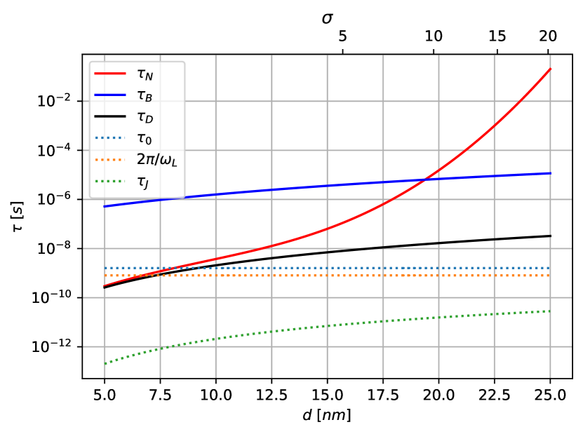
Figure 3: Characteristic timescales involved in relaxation processes associated with ensembles of magnetic nanoparticles. Timescales are calculated for magnetite ($M_{s}=480\;kA/m;K=10\;kJ/m^{3}$), as a function of particle size and temperature, where we choose $\alpha=0.08$. The top x-axis is showing what $\sigma$ to qualify particle size (bottom x-axis) with respect to temperature (not shown).

II Results and Discussion

Looking at Fig. 3, one can get a sense of the considerations and constraints that one comes across in simulations studies of magnetic soft matter, where often, the objective is to scrutinise collective properties at long timescales. In this Figure, we plot the dependence of Neél ($\tau_{N}$), Brownian ($\tau_{B}$), internal diffusion ($\tau_{D}$), period of the precession ($2\pi/\omega_{L}$), precession damping ($\tau_{0}$) and inertial decay ($\tau_{j}$) times as functions of magnetite particle diameter $d$. The range of the anisotropy constant $\sigma$ between $5-20$ covers the most commonly studied nanoparticle sizes and materials. If one was to simulate the magnetodynamics of the nanoparticles explicitly, accounting for all their characteristic magnetic relaxation timescales by, for example, using the aforementioned LLG equation [57, 58, 59], it becomes apparent that $\tau_{J}$ is not small enough to be safely ignored. This means, that one must resolve timescales less than picoseconds to be able to include full magnetodynamics in simulation. This is prohibitively low for any simulations studies concerned with bulk properties. So, from practical considerations, one would like to simulate timescales where high frequency processes ($\leq 10^{-8}$) can be safely ignored. However, a competition remains between $\tau_{N}$ and $\tau_{D}$ on the internal relaxation, and $\tau_{B}$ on the external relaxation side. Specifically, within the $5<\sigma<20$ range, there are regions where $\tau_{N}$ and $\tau_{D}$ are comparable within simulation time, to $\tau_{N}$ becoming prohibitively large, if one was to consider relaxation associated with $\tau_{D}$. Understanding the optimal approach to be able to include relevant magnetodynamic processes in this range, is precisely the question we address below.

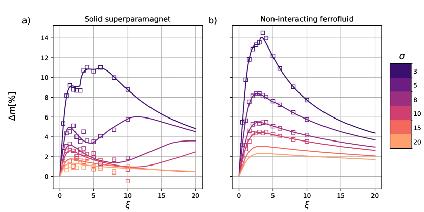
Figure 4: The absolute magnetisation error $\Delta m$ (in percent) between the tSW model (theory–solid line; simulation–symbols) and continuous model descriptions for a solid superparamagnet (subfigure (a)) or a non-interacting ferrofluid (subfigure (b)), as a function of the Langevin parameter $\xi$ and the anisotropy parameter $\sigma$. The colour mapping for $\sigma$ values explored is provided with a colour-bar.

II.1 Static Properties

At a finite temperature, an ensemble of magnetic colloids in a static homogeneous magnetic field is in a thermodynamic equilibrium at times larger than the systems characteristic relaxation time. For any particular configuration of anisotropy axes in a nanoparticle ensemble, the equilibrium state is uniquely defined by ($\sigma$, $\xi$). In Fig. 4, we scrutinise the tSW model in its ability to correctly reproduce equilibrium magnetisation, $m$, of an ensemble of magnetic nanoparticles. The equilibrium magnetization of the system is the total sum of the magnetic moments $\mu$, projected onto the axis of the applied magnetic field. As previously mentioned, we distinguish cases where the particles exhibit either only Néel (solid superparamagnetic) or both Brownian and Néel (non-interacting ferrofluid) relaxation mechanisms.

Within the tSW model, the discrete states in which the magnetic moment can be for a solid superparamagnet, correspond to the energy minima in the total magnetic energy (Eq. 1). The equilibrium magnetisation can be obtained if one performs a summation over a set of allowed discrete orientations:

$$m_{H}^{tSW}=\frac{\sum_{i}\cos\theta_{min,i}\exp\big{[}-U(\theta_{min,i})/k_{B}T\big{]}}{\sum_{i}\exp\big{[}-U(\theta_{min,i})/k_{B}T\big{]}},$$ (14)

where $\theta_{min,i}$ are orientations minimizing the energy at given values of $\xi$, $\sigma$ and $\psi$, $i=1,2$ is the number of a corresponding minimum. To get the magnetization of an ensemble with randomly distributed anisotropy axes, one needs to average $m_{H}^{tSW}$ over all possible orientations of $\vec{n}$:

$$m^{tSW}=\int^{\pi/2}_{0}m_{H}^{tSW}(\xi,\sigma,\psi)\sin\psi\text{d}\psi.$$ (15)

The integral in Eq. 15 can be calculated if we consider components parallel and perpendicular to the applied field direction separately ($h<1$), $m^{tSW}_{\parallel}$ and $m^{tSW}_{\perp}$, respectively, where:

$$m^{tSW}_{\parallel} =\tanh\xi,$$ (16)

$$m^{tSW}_{\perp} =\xi/2\sigma.$$

The problem of describing the equilibrium magnetisation of an ensemble of immobilized, non-interacting, randomly oriented uniaxial particles, has been solved based on a generalization of the Langevin function for the case of solid dispersions with random orientation texture [60, 61, 62]. The full expression together with an outline of the derivation are provided in the Appendix A.

In the case of a non-interacting ferrofluid, $\vec{n}$ and $\vec{e}$ are no longer independent variables - in the tSW model, there exists a unique set of allowed magnetic moment orientations, for any given orientation of the anisotropy axis. The equilibrium magnetisation can be obtained in a similar form to Eq. 15, where:

$$m^{tSW}=\int^{\pi/2}_{0}m_{H}^{tSW}(\xi,\sigma,\psi)f_{n}^{tSW}(\xi,\sigma,\psi)\sin\psi\text{d}\psi,$$ (17)

$$f_{n}^{tSW}(\xi,\sigma,\psi)=\frac{\sum_{i}\exp\big{[}-U(\theta_{min,i}(\psi))/k_{B}T\big{]}}{\int^{\pi/2}_{0}\Big{(}\sum_{i}\exp\big{[}-U(\theta_{min,i}(\psi))/k_{B}T\big{]}\Big{)}\sin\psi\text{d}\psi}.$$

For $\xi=0$, the distribution is random and $f_{n}^{tSW}=1$. In general, however, the magnetization of a non-interacting ferrofluid is given by the Langevin function [34], and does not depend on the anisotropy parameter $\sigma$.

Looking at Fig. 4, one can see that the absolute magnetisation error $\Delta m=|m^{tSW}-m^{sim}|$ demonstrates that the tSW model can reproduce the equilibrium magnetisation within a few percent of the ground truth, in all cases except for particle sizes and/or temperatures where $\sigma\leq 5$, where one can expect a purely super-paramagnetic response. Below this $\sigma$ range, we encounter the limitations of the model. Let us address these limitations. In a solid superparamagnet, the only relaxation mechanism that the particles can leverage to reach equilibrium is Néel.

In the tSW model, there is only a single state in which the dipole moment can be above $h_{cr}$. In other words, the tSW model is equivalent to the classical SW model above $h_{cr}$. In general, however, the magnetic moment orientation can fluctuate relative to the states allowed in the classical SW model [60, 61, 62]. The frequency of these intrawell fluctuations is inversely proportional to $\sigma$. With this in mind, one can understand why the tSW model overestimates the equilibrium magnetisation of low $\sigma$ particles in the large $\xi$ region. Moreover, the intrawell modes matter for high $\xi$ regardless of $\sigma$, as Néel relaxation ($1/p_{1}$) is no longer sufficient for an accurate description of magnetic relaxation [63, 36]. Hence, we observe regions with a slight increase in $\Delta m$ with growing $\xi$. Finally, the importance of intrawell states relative to interwell states increases with decreasing $\xi$, since the applied field is not strong enough to constrain the dipole moment fluctuations perpendicular to the anisotropy axis.

Moving on to the non-interacting ferrofluid system, where both Néel and Brownian relaxation are at play, the same conclusions largely hold, as for a solid superparamagnet. However, one can note a marginally worse agreement between the tSW model and the continuum-level description. Consider the high $\xi$ region, where one can assume Néel relaxation plays a minimal role. For high $\sigma$, we have seen that for a fixed random distribution of the anisotropy axis, the SW reproduces the equilibrium state very well. In the same circumstances, given a non-random distribution of anisotropy axis, the relative error is almost quadrupled. The relative error being different between the left and right subplot in Fig. 4, is related to the fact that, for a solid superparamagnet, the anisotropy axis orientations are randomly distributed and fixed, whereas for a ferrofluid this is not the case. The classical SW model estimates the equilibrium magnetisation incorrectly, but not equally incorrectly for all anisotropy axis distributions. In fact, it can be inferred by comparing the left and right side subplots in Fig. 4, that the more the anisotropy axes are aligned with the magnetic field, the worse is the equilibrium state estimation in the classical SW model.

Finally, it is worth highlighting a particularity of the tSW model, related to the initial susceptibility for low $\sigma$. Initial magnetic susceptibility is an important characteristic of the material linear response to a weak applied field (or “probing field”):

$$\chi=\frac{\partial m}{\partial H}\Big{|}_{H\rightarrow 0}.$$

It can be shown that in the tSW model, the total static susceptibility is given by:

$$\chi^{tSW}(0)=\chi_{L}(1+1/\sigma).$$ (18)

In the limit of no particle anisotropy, the static susceptibility should correspond to the Langevin susceptibility. However, this is not the case in the tSW model, where the values diverge. Although the tSW model reproduces the characteristic internal relaxation time related with Néel relaxation well, it is inadequate for simulations of small enough nanoparticles, or at high enough temperatures where $\sigma<5$.

Having addressed the limitation of the tSW at length, it is important to note that the absolute error for $\sigma\geq 5$ remains less than $10\%$, which qualifies the tSW approach as surprisingly accurate within a wide ($\sigma,\xi$) range of applicability. It is apparent that the dominant internal relaxation mechanism is the Néel one, even for relatively small $\sigma$. Furthermore, our implementation of the tSW is in agreement with the theoretical prediction for the model across the board. The key insight here is that the validity of the tSW model is most constrained by the limitations of the classical SW model, which are well understood and documented. The discrepancies stemming from the lack of intrawell modes are less important, and we do not see this as a substantial additional limitation to the model. Moreover, as long as one is considering non-interacting systems, one can compensate for the overestimation stemming from the classical SW model by tuning the saturation magnetisation of the colloids to fit the correct equilibrium magnetisation curves.

In summary, the tSW model is a reasonably accurate approach to introduce internal magnetisation dynamics for $\sigma\geq 5$ nanoparticles via Néel relaxation, that can reproduce the correct equilibrium in this $\sigma$ range. Having established that, the discussion can proceed to the study of dynamics, which is the type of study where the tSW model can benefit researchers interested in long timescales and bulk sized systems.

II.2 Dynamic Properties

One of the key collective properties of any magnetic soft matter system is its characteristic magnetic relaxation time. This is especially relevant for systems designed for heating applications. The magnetic relaxation time can be assessed by calculating the dynamic susceptibility spectra and locating the maximum/maxima of the susceptibilities imaginary part.

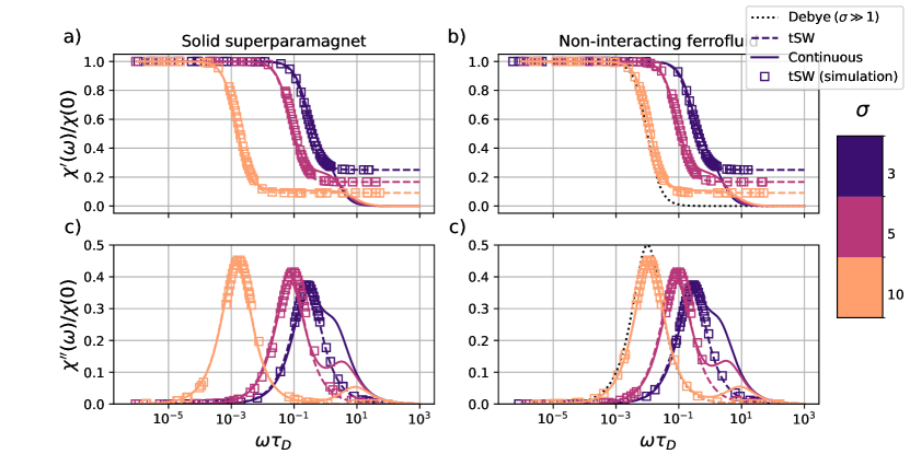
Figure 5: Dynamic susceptibilities for a solid superparamagnet (left column) and non-interacting ferrofluid (right column) as a function of $\omega\tau_{D}$, where $\tau_{D}/\tau_{B}=0.02$. The real and imaginary parts of the susceptibility are shown separately (top and bottom rows, respectively) for clarity. In each subplot, profiles for a continuum description, theoretical and simulation tSW model results are superimposed (see legend), for different values of $\sigma$ (see colourbar).

Let us consider an ensemble of immobilized, non-interacting, randomly oriented particles with uniaxial magnetic anisotropy. In a harmonically oscillating field $H=H_{0}\cos\omega t$, where $t$ is the time and $\omega$ is the oscillation frequency, the magnetisation can generally be represented as a series:

$$m(t)=\sum_{k=1}^{\infty}\left(m^{\prime}_{k}(\omega)\cos k\omega t+m^{\prime\prime}_{k}(\omega)\sin k\omega t\right),$$

where $m^{\prime}$ and $m^{\prime\prime}$ are the Fourier coefficients. In the linear response regime, $H_{0}\rightarrow 0$, only the first harmonic, $k=1$, remains. Here, the dynamic complex susceptibility can be introduced as

$$\chi(\omega)=\chi^{\prime}(\omega)+i\chi^{\prime\prime}(\omega),$$ (19)

where:

$$\chi^{\prime}(\omega)=m^{\prime}_{1}(\omega)/H_{0},\>\>\chi^{\prime\prime}(\omega)=m^{\prime\prime}_{1}(\omega)/H_{0}.$$

For each particle, the susceptibility can be split into components parallel and perpendicular to its anisotropy axis, $\chi_{\parallel}$ and $\chi_{\perp}$, respectively. Assuming that a probing field $|\vec{H}|=H$ is in a $xz$-plane and forms an angle $\psi$ with an easy axis, the magnetization in the linear regime is given by:

$$\vec{m}=(\chi_{\perp}H\sin\psi,0,\chi_{\parallel}H\cos\psi),$$

where, the total particle susceptibility obeys the superposition rule [52]:

$$\chi=\left(\frac{1}{3}\chi_{\parallel}+\frac{2}{3}\chi_{\perp}\right)$$

This relation must be true for both the static and dynamic case. For immobilized particles, within the continuous approach and without gyromagnetic effects [52]:

$$\chi_{\parallel}(\omega)\simeq\frac{\chi_{\parallel}(0)}{1-i\omega\tau_{\parallel}},\>\>\>\chi_{\parallel}(0)=\chi_{L}(1+2S), \>\>\>\tau_{\parallel}=\tau_{D}\frac{e^{\sigma}-1}{2\sigma}\left[\frac{1}{1+1/\sigma}\sqrt{\frac{\sigma}{\pi}}+2^{-\sigma-1}\right]^{-1};$$ (20)

$$\chi_{\perp}(\omega)\simeq\frac{\chi_{\perp}(0)}{1-i\omega\tau_{\perp}},\>\>\>\chi_{\perp}(0)= \chi_{L}(1-S),\>\>\>\tau_{\perp}=2\tau_{D}\frac{1-S}{2+S},$$

where the order parameter $S$ is given by:

$$S=\frac{3}{4}\frac{1}{\sigma}\Bigg{[}\frac{\sqrt{\sigma}}{D\big{(}\sqrt{\sigma}\big{)}}-1\Bigg{]}-\frac{1}{2},$$ (21)

$D$ is the Dawson function:

$$D(x)=e^{-x^{2}}\int_{0}^{x}e^{t^{2}}\,\text{d}t,$$

and $\chi_{L}$ is the static susceptibility of an isotropic superparamagnet (Langevin susceptibility):

$$\chi_{L}=\frac{\mu_{0}\mu^{2}N}{3Vk_{B}T}.$$ (22)

In the case where particles are not immobilised, it is sufficient to replace relaxation times with effective values [64]:

$$\tau^{*}_{\parallel}=\left(\tau^{-1}_{\parallel}+\tau_{B}^{-1}\right)^{-1},\\ \tau^{*}_{\perp}=\left(\tau^{-1}_{\perp}+\tau_{B}^{-1}\right)^{-1}.$$

In the tSW model, the relaxation time $\tau_{\parallel}$ is an input parameter, which means that the dynamics of tSW parallel to the easy axis must be the same as in the continuous case. The orthogonal relaxation time $\tau_{\perp}$ is instantaneous. Therefore, the dynamic susceptibility of an ensemble of frozen, uniaxial magnetic nanoparticles with a random distribution of anisotropy axis is given by:

$$\chi^{tSW}(\omega)=\frac{\chi_{L}}{1-i\omega\tau_{\parallel}}+\frac{\chi_{L}}{\sigma}.$$ (23)

Once again, for a liquid, it is sufficient to introduce effective relaxation times: $\tau_{\parallel}\rightarrow\tau^{*}_{\parallel}$. Note, that the orthogonal magnetic response (which is instantaneous and does not have any fluctuations associated with it) will not make any contribution to the zero-field magnetization autocorrelation function. Therefore, the calculated susceptibilities from the autocorrelation function when using the tSW method will be incorrect. The simulated susceptibilities have been calculated by applying a weak oscillating magnetic field (maximum amplitude corresponding to $\xi=0.1$) for a span of frequencies, in order to be able to determine the complex susceptibilities from the time evolution of the total magnetisation vector (see Eq.19). Similarly, the static susceptibilities should be estimated from the initial slope in the magnetisation profiles.

Looking at Fig. 5, we can see that the tSW model reproduces the correct dynamics in both the solid superparamagnet and non-interacting ferrofluid systems, as quantified by the initial dynamic susceptibilities. Of course, in the initial susceptibility regime, the tSW model incorporated dipole moment fluctuations only along the anisotrpy axis associated with $\tau_{\parallel}$, which in this case is equivalent to $\tau_{N}$. Since this is an input parameter for the model, the tSW can confidently reproduce the correct internal dynamics for the lowest frequency relaxation process ($\tau_{\parallel}$). It is apparent that Néel relaxation is very relevant even for $\sigma=10$ particles, where the dynamic susceptibility is clearly distinct from the Debye limit shown with dots. Recall that the maximum of the Debye limit is at $\omega\tau_{d}=0.01$, which is set by the model as $\tau_{D}/\tau_{N}=0.01$. The high frequency peaks, resolved in the continuum description, corresponding to $\tau_{\perp}$, cannot be captured in the tSW, simply due to the fact that there are no fluctuations associated perpendicular to the anisotropy axis in the $H\rightarrow 0$ regime. Outside of the initial susceptibility regime, this is not an issue as the dipole moment instantaneously follows the local energy minima, as obtained in the classical SW model, where there is always a relative angle the dipole moment takes with respect to the anisotropy axis. However, within the range of applicability we suggest ($\sigma>5$), these higher frequency processes are distinct enough that they could be averaged out while still resolving the correct dynamics. Having said that, it should also be clear that the in-field susceptibility contribution perpendicular to the anisotropy axis is frequency independent.

As suggested at the beginning of this section, the position(s) of the maxima of the imaginary part of the initial susceptibility indicate the optimal field frequencies for heating applications. Fig. 5 clearly shows that if one needs to optimise the frequency of an applied magnetic field for hyperthermia depending on the particle size and material, using a point dipole approximation can be very misleading, as even for rather high anisotropy energies, the shape and the imaginary part of the susceptibility spectra drastically differ from that of a purely Brownian, or purely Neél relaxing systems.

In summary, we can see that the tSW approach can confidently be used to incorporate Néel relaxation and simulate the dynamics associated with that relaxation process for magnetic nanoparticles with $\sigma\geq 5$. This is also the first major use case where we see that this model could enable new simulation studies. The price to pay in terms of accuracy is slight, compared to the simulation scale compromises that would be unavoidable with an approach that reproduces also the higher frequency relaxation processes. The second major use case of the tSW model would be to simulate systems where $\tau_{B}$ is high. In this case, a Brownian dynamics approach to thermalise each particle might be impractical. A good example here would be multicore or composite magnetic colloids, where the nanoparticles are embedded in a solid matrix[65, 66, 67].

III Conclusions

Driven by a long-standing need to introduce the internal magnetization dynamics into coarse-grained computer simulations of magnetic soft matter, we proposed an approach that is able to encompass both Neél and Brownian relaxations in a computationally affordable manner. In this paper, we introduce the Stoner-Wohlfarth thermal model (tSW) and validate it against an ensemble of immobilized, non-interacting, randomly oriented uniaxial particles (solid superparamagnet) and a classical dilute (non-interacting) ferrofluid for various combinations of anisotropy strength and Zeeman energy at a fixed temperature. In order to find the range of validity of our approach, we compared its predictions to the analytical results. The availability of the latter, in fact, defined the choice of the systems to model for this work.

It was crucial to verify whether the newly formulated tSW model is able to reproduce both the equilibrium and dynamic properties of magnetic soft matter systems. Our findings indicate that the tSW model is applicable and efficient when the anisotropy of a particle exceeds thermal fluctuations by a factor of four to five and above.

Our work opens possibilities for future investigations of magnetic soft matter systems in which the interplay between internal magnetization degrees of freedom and Brownian rotation is often overlooked.

IV Methodology

IV.1 Simulation Method

We perform MD simulations of a solid superparamagnet and a non-interacting ferrofluid for different anisotropy and Langevin parameter combinations $(\sigma,\xi)$, at a fixed temperature, using the ESPResSo simulation package [68]. Magnetic nanoparticles are assumed to be mono-disperse, spherical particles with a point dipole, and a characteristic diameter $\Omega$. The solvent was implicitly represented via the Langevin thermostat[69]. The equations of motion are integrated over time $t$ numerically:

$$M_{i}\frac{d\vec{\mbox{$\nu$}}_{i}}{dt}=\vec{\mbox{F}}_{i}-\Gamma_{Tl}\vec{\mbox{$\nu$}}_{i}+2\vec{\mbox{$\xi$}}_{i}^{Tl},$$ (24)

$$I_{i}\frac{d\vec{\mbox{$\omega$}}_{i}}{dt}=\vec{\mbox{$\tau$}}_{i}-\Gamma_{R}\vec{\mbox{$\omega$}}_{i}+2\vec{\mbox{$\xi$}}_{i}^{R},$$ (25)

where for the $i$-th particle in Eq. (24), $M_{i}$, is, in general, a rank two mass tensor. Since we are simulating isotropic colloids, the mass tensor reduces to a scalar. $\vec{\mbox{F}}_{i}$ is the force acting on the particle; $\vec{\mbox{$\nu$}}_{i}$ denotes the translational velocity. $\Gamma_{Tl}$ denotes the translational friction tensor that once again, due to the isotropy arguments, reduces to a scalar friction coefficient. Finally, $\vec{\mbox{$\xi$}}_{i}^{Tl}$ is a stochastic force, modelling the thermal fluctuations of the implicit solvent. Similarly, in Eq. (25), $I_{i}$ denotes $i$-th particle inertia tensor (scalar for a homogeneous sphere), $\vec{\mbox{$\tau$}}_{i}$ is torque acting on it, $\vec{\mbox{$\omega$}}_{i}$ is particle rotational velocity. As for the translation, $\Gamma_{R}$ denotes the rotational friction tensor that reduces to a scalar for our colloids, and the $\vec{\mbox{$\xi$}}_{i}^{R}$ is a stochastic torque serving for the same purpose as $\vec{\mbox{$\xi$}}_{i}^{Tl}$. Both stochastic terms satisfy the conditions on their time averages [70]:

$$\langle\vec{\mbox{$\xi$}}^{Tl/R}\rangle_{t} =0$$

$$\langle\vec{\mbox{$\xi$}}_{l}^{Tl/R}(t)\vec{\mbox{$\xi$}}_{k}^{Tl/R}(t^{\prime})\rangle =2\Gamma_{Tl/R}k_{B}T\delta_{l,k}\delta(t-t^{\prime});$$

where $k,l=x,y,z$.

Forces and torques in Eqs. (24) and (25) are calculated from interaction potentials. We used periodic boundary conditions, to avoid finite-size effects. Integration of the equations of motion was performed using the velocity Verlet algorithm [71], with a timestep of 0.01 (see IV.2 for more detail on the simulation units and their relation to experimental values). The tSW calculation, as described in Section I.3, is done before the force calculation in the velocity Verlet scheme. The initial configuration on our simulations is constructed by randomly placing 500 particles in a cubic simulation box, where the anisotropy axis orientations were uniformly distributed on a surface of a sphere. Simulations length was chosen to be 100$\tau_{char}$, where $\tau_{char}$ denotes the characteristic time of the longest relaxation process we needed to resolve. To obtain statistically significant results, we always present averages over eight independent simulation runs, and over 20 statistically independent snapshots for each simulation. We include the Zeeman energy from the external magnetic field $\vec{H}$:

$$U_{H}=-\mu_{0}\sum_{i=0}^{N}\vec{H}\cdot\vec{\mu}_{i}.$$ (26)

The performance and reliability of the implementation of tSW is dependent on a robust and highly efficient strategy to find the extrema in Eq.5. For this purpose, we make use of Nlopt, a free/open-source library for nonlinear optimization [72]. Nlopt is a versatile library written in C, with a common interface for a multitude of different optimization strategies. We have specifically settled on using the Method of Moving Asymptotes (MMA) algorithm [73] to find extrema in Eq.5. MMA is guaranteed to converge to some local minimum and has, throughout our testing, proven to be well suited for optimisation of Eq.5, converging to the correct energy minima very quickly.

IV.2 Reduced units and mapping to physical parameters

In this subsection, we give an overview of the SI and reduced units used in our simulations. The units are presented in the order we find most instructive. We start with a common reference material choice for the magnetic nanoparticles, namely, magnetite. We assumed that magnetite has uniaxial anisotropy with a magnetic anisotropy constant of $K=10\;kJ/m^{3}$, saturation magnetisation $M_{s}=480\cdot 10^{3}\;kg/(ms^{2})$ and a core density $\rho_{m}=5170kg/m^{3}$. The uniaxial anisotropy assumption is commonly used, but is not strictly correct, as pointed out in Witt et al. [74]. In all cases, we assumed that the magnetite core is coated with a 2 nm thick oleic acid coating (density $895kg/m^{3}$). Given a value of $\sigma$ we want to explore, considering the material values given above, the unit length is chosen to be the diameter of the nanoparticle and a unit mass is chosen to be its mass. We choose the particle volume fraction in the simulation box to be $\phi=0.001$. The side length of the simulation box was set to $\approx 64\Omega$, derived based on the chosen $\phi$ and the particle number. In all cases, we choose the unit energy to be room temperature $T=298.15K$. In other words, we set the reduced temperature of the Langevin thermostat to $k_{B}T=1$. These three choices also uniquely determine the unit time. From there, we calculate $\tau_{D}$, where the gyromagnetic ratio is $\mu_{0}\cdot(1.76\cdot 10^{11}\;s^{-1}T^{-1})$, the damping parameter is chosen to be $\alpha=0.08$ and $\mu_{0}$ is the vacuum permittivity. We choose $\tau_{D}/\tau_{B}=0.01$. Based on this choice, we can derive the density of the implicit fluid and the respective rotational and translational friction coefficients.

V Appendix A

Here, we derive the equilibrium magnetisation for an ensemble of immobilized, non-interacting, randomly oriented uniaxial particles. First, let us consider immobilized particles with a predefined orientation of the anisotropy axes ($\vec{n}=const$).The equilibrium projection of magnetization on the field direction is

$$m_{H}=\langle\cos\theta\rangle_{eq}=\int\cos\theta\>W_{eq}\>\text{d}\vec{e},$$ (27)

where $\int\ldots d\vec{e}$ is the integral over all possible orientations of the magnetic moment and $W_{eq}$ is the equilibrium (Gibbs/Boltzmann) PDF,

$$W_{eq}=\frac{\exp\big{(}-U/k_{B}T\big{)}}{Z(\xi,\sigma,\vec{n})}$$ (28)

$Z$ is the partition function,

$$Z(\xi,\sigma,\vec{n}) =\int\exp\big{(}-U/k_{B}T\big{)}\text{d}\vec{e}$$ (29)

$$=\int\exp\big{[}\xi\cos\theta+\sigma\left(\vec{e}\cdot\vec{n}\right)^{2}\big{]}\text{d}\vec{e}.$$

Combining Eq. 28 and Eq. 29:

$$m_{H}=\frac{\partial_{\xi}Z(\xi,\sigma,\vec{n})}{Z(\xi,\sigma,\vec{n})}.$$ (30)

In practice, it is easier to consider integral Eq. 29 in a spherical coordinate system, in which $z$-axis coincides with the easy axis and the field lies perpedicular to the $xz$-plane, i.e., $\vec{n}=(0,0,1)$ and $\vec{H}=H(\sin\psi,0,\cos\psi)$. Let us denote magnetic moment angles in this system as $\phi_{n}$ and $\theta_{n}$, so $\vec{e}=(\cos\phi_{n}\sin\theta_{n},\sin\phi_{n}\sin\theta_{n},\cos\theta_{n})$. Note, in the main text, it was an external field that was aligned along the $z$-axis, and the easy axis was forming an angle $\psi$ with it in the $xz$-plane. Then Eq.29 becomes:

$$Z(\xi,\sigma,\psi) =\int^{2\pi}_{0}\text{d}\phi\int^{\pi}_{0}\exp\big{[}\sigma\cos^{2}\theta_{n}+\xi(\cos\theta_{n}\cos\psi+\cos\phi_{n}\sin\theta_{n}\sin\psi)\big{]}\sin\theta_{n}\text{d}\theta_{n}$$ (31)

$$=\int^{\pi}_{0}\exp\big{(}\sigma\cos^{2}\theta_{n}+\xi\cos\theta_{n}\cos\psi\big{)}\Bigg{(}\int^{2\pi}_{0}\exp\big{[}\xi\cos\phi_{n}\sin\theta_{n}\sin\psi\big{]}\text{d}\phi_{n}\Bigg{)}\sin\theta_{n}\text{d}\theta_{n}$$

$$=2\pi\int^{1}_{-1}\exp\big{(}\sigma x^{2}\big{)}\exp\big{(}\xi\cos\psi\>x\big{)}I_{0}\Bigg{(}\xi\sin\psi\sqrt{1-x^{2}}\Bigg{)}\text{d}x$$

$$=2\pi\int^{1}_{-1}\exp\big{(}\sigma x^{2}\big{)}\Big{[}\cosh\big{(}\xi\cos\psi\>x\big{)}+\sinh\big{(}\xi\cos\psi\>x\big{)}\Big{]}I_{0}\Bigg{(}\xi\sin\psi\sqrt{1-x^{2}}\Bigg{)}\text{d}x$$

$$=4\pi\int^{1}_{0}\exp\big{(}\sigma x^{2}\big{)}\cosh\big{(}\xi\cos\psi\>x\big{)}I_{0}\Bigg{(}\xi\sin\psi\sqrt{1-x^{2}}\Bigg{)}\text{d}x.$$

where $I_{0}$ is the modified Bessel function of the first kind of order zero. Analogous expressions for the partition function of an immobilized particle can be found in Refs. [75, 34]. The derivative is given by:

$$\partial_{\xi}Z(\xi,\sigma,\psi)=4\pi\int^{1}_{0}\exp\big{(}\sigma x^{2}\big{)}\Bigg{[} x\cos\psi\sinh\big{(}\xi\cos\psi\>x\big{)}I_{0}\bigg{(}\xi\sin\psi\sqrt{1-x^{2}}\bigg{)}+$$ (32)

$$\sqrt{1-x^{2}}\sin\psi\cosh\big{(}\xi\cos\psi\>x\big{)}I_{1}\bigg{(}\xi\sin\psi\sqrt{1-x^{2}}\bigg{)}\Bigg{]}\text{d}x,$$ (33)

where $I_{1}$ is the modified Bessel function of the first kind of order one. To get the magnetization of an ensemble with randomly distributed easy axes, one needs to average $m_{H}$ over all possible orientations of $\vec{n}$.

$$m =\frac{1}{4\pi}\int m_{H}(\xi,\sigma,\vec{n})\text{d}\vec{n}\ =\ \frac{1}{4\pi}\int^{2\pi}_{0}\text{d}\zeta\times$$ (34)

$$\times\int^{\pi}_{0}m_{H}(\xi,\sigma,\psi)\sin\psi\text{d}\psi=\int^{\pi/2}_{0}m_{H}(\xi,\sigma,\psi)\sin\psi\text{d}\psi.$$

The transition $\int^{\pi}_{0}\text{d}\psi\rightarrow 2\int^{\pi/2}_{0}\text{d}\psi$ can be made because the integrand is symmetrical with respect to $\cos\psi$. Also note, that since there is no special direction in the plane orthogonal to the field, the magnetization of a random ensemble must be strictly aligned with the field and the perpendicular component of magnetization must be zero (this is why subscript $H$ can be omitted).

References

- Langevin [1905a] P. Langevin, Sur la theory du magnetism, J. de Phys. 4, 678 (1905a).
- Langevin [1905b] P. Langevin, Magnetism et theory des electrons, Ann. Chim. et Phys. 5, 70 (1905b).
- Elmore [1938] W. C. Elmore, The magnetization of ferromagnetic colloids, Phys. Rev. 54, 1092 (1938).
- L. Resler Jr. and R. E. Rosensweig [1964] L. Resler Jr. and R. E. Rosensweig, Magnetocaloric power, J. AIAA 2, 1418 (1964).
- Resler and Rosensweig [1964] E. Resler and R. Rosensweig, Magnetocaloric power, AIAA Journal 2, 1418 (1964).
- Cebers et al. [1997] A. Cebers, E. Blum, and M. Maiorov, Magnetic fluids, Walter de 646 (1997).
- Odenbach [2008] S. Odenbach, Ferrofluids: magnetically controllable fluids and their applications, Vol. 594 (Springer, 2008).
- Odenbach [2009] S. Odenbach, ed., Colloidal Magnetic Fluids, Lecture Notes in Physics, Vol. 763 (Springer-Verlag, Berlin Heidelberg, 2009).
- Zrınyi et al. [1998] M. Zrınyi, D. Szabó, and H.-G. Kilian, Kinetics of the shape change of magnetic field sensitive polymer gels, Polymer Gels and Networks 6, 441 (1998).
- Weeber et al. [2018] R. Weeber, M. Hermes, A. M. Schmidt, and C. Holm, Polymer architecture of magnetic gels: a review., Journal of physics. Condensed matter: an Institute of Physics journal 30, 063002 (2018).
- Volkova et al. [2017] T. Volkova, V. Böhm, T. Kaufhold, J. Popp, F. Becker, D. Y. Borin, G. Stepanov, and K. Zimmermann, Motion behaviour of magneto-sensitive elastomers controlled by an external magnetic field for sensor applications, Journal of Magnetism and Magnetic Materials 431, 262 (2017).
- Filipcsei et al. [2007] G. Filipcsei, I. Csetneki, A. Szilágyi, and M. Zrínyi, Magnetic field-responsive smart polymer composites, in Oligomers-Polymer Composites-Molecular Imprinting (Springer, 2007) pp. 137–189.
- Li et al. [2014] Y. Li, J. Li, W. Li, and H. Du, A state-of-the-art review on magnetorheological elastomer devices, Smart materials and structures 23, 123001 (2014).
- Odenbach [2016] S. Odenbach, Microstructure and rheology of magnetic hybrid materials, Archive of Applied Mechanics 86, 269 (2016).
- Sánchez et al. [2019] P. A. Sánchez, E. S. Minina, S. S. Kantorovich, and E. Y. Kramarenko, Surface relief of magnetoactive elastomeric films in a homogeneous magnetic field: molecular dynamics simulations, Soft matter 15, 175 (2019).
- Frank and Lauterbur [1993] S. Frank and P. C. Lauterbur, Voltage-sensitive magnetic gels as magnetic resonance monitoring agents, Nature 363, 334 (1993).
- Weeber et al. [2012] R. Weeber, S. Kantorovich, and C. Holm, Deformation mechanisms in 2d magnetic gels studied by computer simulations, Soft Matter 8, 9923 (2012).
- Dreyfus et al. [2005] R. Dreyfus, J. Baudry, M. L. Roper, M. Fermigier, H. A. Stone, and J. Bibette, Microscopic artificial swimmers, Nature 437, 862 (2005).
- Benkoski et al. [2008] J. J. Benkoski, S. E. Bowles, R. L. Jones, J. F. Douglas, J. Pyun, and A. Karim, Self-assembly of polymer-coated ferromagnetic nanoparticles into mesoscopic polymer chains, J Polym Sci, Part B: Polym Phy 46, 2267 (2008).
- Gubin [2009] S. P. Gubin, Magnetic nanoparticles (John Wiley & Sons, 2009).
- Ivanov and Camp [2023] A. O. Ivanov and P. J. Camp, Magnetization relaxation dynamics in polydisperse ferrofluids, Physical Review E 107, 034604 (2023).
- Mostarac and Kantorovich [2022] D. Mostarac and S. S. Kantorovich, Rheology of a nanopolymer synthesized through directional assembly of dna nanochambers, for magnetic applications, Macromolecules 55, 6462 (2022).
- Mostarac et al. [2022] D. Mostarac, Y. Xiong, O. Gang, and S. Kantorovich, Nanopolymers for magnetic applications: how to choose the architecture?, Nanoscale 14, 11139 (2022).
- Novikau et al. [2022] I. S. Novikau, E. V. Novak, E. S. Pyanzina, and S. S. Kantorovich, Behaviour of a magnetic nanogel in a shear flow, Journal of Molecular Liquids 346, 118056 (2022).
- Rosenberg and Kantorovich [2023] M. Rosenberg and S. Kantorovich, The influence of anisotropy on the microstructure and magnetic properties of dipolar nanoplatelet suspensions, Physical Chemistry Chemical Physics 25, 2781 (2023).
- Coffey and Kalmykov [2012] W. T. Coffey and Y. P. Kalmykov, Thermal fluctuations of magnetic nanoparticles: Fifty years after brown, Journal of Applied Physics 112 (2012).
- Buyevich and Ivanov [1992] Y. A. Buyevich and A. Ivanov, Equilibrium properties of ferrocolloids, Physica A: Statistical Mechanics and its Applications 190, 276 (1992).
- Stoner and Wohlfarth [1948] E. C. Stoner and E. Wohlfarth, A mechanism of magnetic hysteresis in heterogeneous alloys, Philosophical Transactions of the Royal Society of London. Series A, Mathematical and Physical Sciences 240, 599 (1948).
- Néel [1949] L. Néel, Influence des fluctuations thermiques sur l’aimantation de grains ferromagnétiques très fins, Comptes Rendus Hebdomadaires Des Seances De L Academie Des Sciences 228, 664 (1949).
- Brown [1963] W. F. Brown, Thermal fluctuations of a single-domain particle, Phys. Rev. 130, 1677 (1963).
- Taukulis and Cebers [2012] R. Taukulis and A. Cebers, Coupled stochastic dynamics of magnetic moment and anisotropy axis of a magnetic nanoparticle, Phys. Rev. E 86, 061405 (2012).
- Ilg [2017] P. Ilg, Equilibrium magnetization and magnetization relaxation of multicore magnetic nanoparticles, Phys. Rev. B 95, 214427 (2017).
- Bender et al. [2018] P. Bender, J. Fock, C. Frandsen, M. F. Hansen, C. Balceris, F. Ludwig, O. Posth, E. Wetterskog, L. K. Bogart, P. Southern, W. Szczerba, L. Zeng, K. Witte, C. Grüttner, F. Westphal, D. Honecker, D. González-Alonso, L. Fernández Barquín, and C. Johansson, Relating magnetic properties and high hyperthermia performance of iron oxide nanoflowers, J. Phys. Chem. C 122, 3068 (2018), https://doi.org/10.1021/acs.jpcc.7b11255 .
- Elfimova et al. [2019] E. A. Elfimova, A. O. Ivanov, and P. J. Camp, Static magnetization of immobilized, weakly interacting, superparamagnetic nanoparticles, Nanoscale 11, 21834 (2019).
- Ilg and Kröger [2022] P. Ilg and M. Kröger, Longest relaxation time versus maximum loss peak in the field-dependent longitudinal dynamics of suspended magnetic nanoparticles, Phys. Rev. B 106, 134433 (2022).
- Poperechny [2023] I. Poperechny, Multipeak dynamic magnetic susceptibility of a superparamagnetic nanoparticle suspended in a fluid, Physical Review B 107, 064416 (2023).
- Ménager et al. [2004] C. Ménager, O. Sandre, J. Mangili, and V. Cabuil, Preparation and swelling of hydrophilic magnetic microgels, Polymer 45, 2475 (2004).
- Backes et al. [2015] S. Backes, M. U. Witt, E. Roeben, L. Kuhrts, S. Aleed, A. M. Schmidt, and R. von Klitzing, Loading of pnipam based microgels with cofe2o4 nanoparticles and their magnetic response in bulk and at surfaces, J. Phys. Chem. B 119, 12129 (2015).
- Mandal et al. [2019] P. Mandal, S. Maji, S. Panja, O. P. Bajpai, T. K. Maiti, and S. Chattopadhyay, Magnetic particle ornamented dual stimuli responsive nanogel for controlled anticancer drug delivery, New J. Chem. 43, 3026 (2019).
- Sung et al. [2021] B. Sung, M.-H. Kim, and L. Abelmann, Magnetic microgels and nanogels: Physical mechanisms and biomedical applications, Bioeng. Transl. Med. 6, e10190 (2021).
- Cao et al. [2020] Y. Cao, Z. Mao, Y. He, Y. Kuang, M. Liu, Y. Zhou, Y. Zhang, and R. Pei, Extremely small iron oxide nanoparticle-encapsulated nanogels as a glutathione-responsive t1 contrast agent for tumor-targeted magnetic resonance imaging, ACS Appl Mater Interfaces 12, 26973 (2020), pMID: 32452664, https://doi.org/10.1021/acsami.0c07288 .
- Gao et al. [2020] F. Gao, X. Wu, D. Wu, J. Yu, J. Yao, Q. Qi, Z. Cao, Q. Cui, and Y. Mi, Preparation of degradable magnetic temperature- and redox-responsive polymeric/fe3o4 nanocomposite nanogels in inverse miniemulsions for loading and release of 5-fluorouracil, Colloids and Surfaces A: Physicochemical and Engineering Aspects 587, 124363 (2020).
- Biglione et al. [2020] C. Biglione, J. Bergueiro, S. Wedepohl, B. Klemke, M. C. Strumia, and M. Calderón, Revealing the nir-triggered chemotherapy therapeutic window of magnetic and thermoresponsive nanogels, Nanoscale 12, 21635 (2020).
- Hilger and Kaiser [2012] I. Hilger and W. A. Kaiser, Iron oxide-based nanostructures for mri and magnetic hyperthermia, Nanomedicine 7, 1443 (2012), pMID: 22994960, https://doi.org/10.2217/nnm.12.112 .
- Dürr et al. [2013] S. Dürr, C. Janko, S. Lyer, P. Tripal, M. Schwarz, J. Zaloga, R. Tietze, and C. Alexiou, Magnetic nanoparticles for cancer therapy, Nanotechnology Reviews 2, 395 (2013).
- Périgo et al. [2015] E. A. Périgo, G. Hemery, O. Sandre, D. Ortega, E. Garaio, F. Plazaola, and F. J. Teran, Fundamentals and advances in magnetic hyperthermia, Appl. Phys. Rev. 2, 041302 (2015).
- Abenojar et al. [2016] E. C. Abenojar, S. Wickramasinghe, J. Bas-Concepcion, and A. C. S. Samia, Structural effects on the magnetic hyperthermia properties of iron oxide nanoparticles, Progress in Natural Science: Materials International 26, 440 (2016), special Issue for Nano Materials.
- Chuev and Hesse [2007] M. Chuev and J. Hesse, Nanomagnetism: extension of the stoner–wohlfarth model within néel’s ideas and useful plots, Journal of Physics: Condensed Matter 19, 506201 (2007).
- Chantrell et al. [2000] R. Chantrell, N. Walmsley, J. Gore, and M. Maylin, Calculations of the susceptibility of interacting superparamagnetic particles, Physical Review B 63, 024410 (2000).
- Poperechny et al. [2014] I. Poperechny, Y. L. Raikher, and V. Stepanov, Dynamic hysteresis of a uniaxial superparamagnet: Semi-adiabatic approximation, Physica B: Condensed Matter 435, 58 (2014).
- García-Palacios and Lázaro [1998] J. L. García-Palacios and F. J. Lázaro, Langevin-dynamics study of the dynamical properties of small magnetic particles, Physical Review B 58, 14937 (1998).
- Raikher and Stepanov [2004] Y. L. Raikher and V. I. Stepanov, Nonlinear dynamic susceptibilities and field-induced birefringence in magnetic particle assemblies, Advances in Chemical Physics 129, 419 (2004).
- Chalifour et al. [2021] A. R. Chalifour, J. C. Davidson, N. R. Anderson, T. M. Crawford, and K. L. Livesey, Magnetic relaxation time for an ensemble of nanoparticles with randomly aligned easy axes: A simple expression, Physical Review B 104, 094433 (2021).
- Raikher and Shliomis [1975] Y. L. Raikher and M. Shliomis, Theory of dispersion of the magnetic susceptibility of fine ferromagnetic particles, Soviet Physics-JETP 40, 526 (1975).
- Kalmykov and Coffey [1997] Y. P. Kalmykov and W. T. Coffey, Transverse complex magnetic susceptibility of single-domain ferromagnetic particles with uniaxial anisotropy subjected to a longitudinal uniform magnetic field, Phys. Rev. B 56, 3325 (1997).
- Raikher and Shliomis [1994] Y. L. Raikher and M. I. Shliomis, The effective field method in the orientational kinetics of magnetic fluids and liquid crystals, Advances in chemical physics: relaxation phenomena in condensed matter 87, 595 (1994).
- Landau and Lifshitz [1992] L. Landau and E. Lifshitz, On the theory of the dispersion of magnetic permeability in ferromagnetic bodies, in Perspectives in Theoretical Physics (Elsevier, 1992) pp. 51–65.
- Gilbert [2004] T. L. Gilbert, A phenomenological theory of damping in ferromagnetic materials, IEEE transactions on magnetics 40, 3443 (2004).
- Helbig et al. [2023] S. Helbig, C. Abert, P. A. Sánchez, S. S. Kantorovich, and D. Suess, Self-consistent solution of magnetic and friction energy losses of a magnetic nanoparticle, Physical Review B 107, 054416 (2023).
- Kuznetsov [2018] A. A. Kuznetsov, Equilibrium magnetization of a quasispherical cluster of single-domain particles, Physical Review B 98, 144418 (2018).
- Williams et al. [1993] H. Williams, K. O’Grady, M. El Hilo, and R. Chantrell, Superparamagnetism in fine particle dispersions, Journal of magnetism and magnetic materials 122, 129 (1993).
- Cregg and Bessais [1999a] P. Cregg and L. Bessais, Series expansions for the magnetisation of a solid superparamagnetic system of non-interacting particles with anisotropy, Journal of magnetism and magnetic materials 202, 554 (1999a).
- Garanin [1997] D. A. Garanin, Fokker-planck and landau-lifshitz-bloch equations for classical ferromagnets, Physical Review B 55, 3050 (1997).
- Shliomis and Stepanov [1994] M. Shliomis and V. Stepanov, Theory of the dynamic susceptibility of magnetic fluids, Advances in Chemical Physics: Relaxation Phenomena in Condensed Matter 87, 1 (1994).
- Eberbeck et al. [2012] D. Eberbeck, C. L. Dennis, N. F. Huls, K. L. Krycka, C. Gruttner, and F. Westphal, Multicore magnetic nanoparticles for magnetic particle imaging, IEEE Transactions on Magnetics 49, 269 (2012).
- Kuznetsov et al. [2022] A. A. Kuznetsov, E. V. Novak, E. S. Pyanzina, and S. S. Kantorovich, Structural and magnetic equilibrium properties of a semi-dilute suspension of magnetic multicore nanoparticles, Journal of Molecular Liquids 359, 119373 (2022).
- Kuznetsov et al. [2023] A. A. Kuznetsov, E. V. Novak, E. S. Pyanzina, and S. S. Kantorovich, Multicore-based ferrofluids in zero field: initial magnetic susceptibility and self-assembly mechanisms, Soft Matter 19, 4549 (2023).
- Weik et al. [2019] F. Weik, R. Weeber, K. Szuttor, K. Breitsprecher, J. de Graaf, M. Kuron, J. Landsgesell, H. Menke, D. Sean, and C. Holm, Espresso 4.0–an extensible software package for simulating soft matter systems, The European Physical Journal Special Topics 227, 1789 (2019).
- Allen and Tildesley [2017] M. P. Allen and D. J. Tildesley, Computer simulation of liquids (Oxford university press, 2017).
- Uhlenbeck and Ornstein [1930] G. E. Uhlenbeck and L. S. Ornstein, On the theory of the brownian motion, Physical review 36, 823 (1930).
- Rapaport [2004] D. C. Rapaport, The art of molecular dynamics simulation (Cambridge university press, 2004).
- Johnson [2007] S. G. Johnson, The NLopt nonlinear-optimization package, https://github.com/stevengj/nlopt (2007).
- Svanberg [2002] K. Svanberg, A class of globally convergent optimization methods based on conservative convex separable approximations, SIAM journal on optimization 12, 555 (2002).
- Witt et al. [2005] A. Witt, K. Fabian, and U. Bleil, Three-dimensional micromagnetic calculations for naturally shaped magnetite: Octahedra and magnetosomes, Earth and Planetary Science Letters 233, 311 (2005).
- Cregg and Bessais [1999b] P. Cregg and L. Bessais, A single integral expression for the magnetisation of a textured superparamagnetic system, Journal of magnetism and magnetic materials 203, 265 (1999b).