Learned Indexes with Distribution Smoothing via Virtual Points

Abstract

Recent research on learned indexes has created a new perspective for indexes as models that map keys to their respective storage locations. These learned indexes are created to approximate the cumulative distribution function of the key set, where using only a single model may have limited accuracy. To overcome this limitation, a typical method is to use multiple models, arranged in a hierarchical manner, where the query performance depends on two aspects: (i) traversal time to find the correct model and (ii) search time to find the key in the selected model. Such a method may cause some key space regions that are difficult to model to be placed at deeper levels in the hierarchy. To address this issue, we propose an alternative method that modifies the key space as opposed to any structural or model modifications. This is achieved through making the key set more learnable (i.e., smoothing the distribution) by inserting virtual points. Further, we develop an algorithm named CSV to integrate our virtual point insertion method into existing learned indexes, reducing both their traversal and search time. We implement CSV on state-of-the-art learned indexes and evaluate them on real-world datasets. The extensive experimental results show significant query performance improvement for the keys in deeper levels of the index structures at a low storage cost.

I Introduction

Learned indexes [1] have reported strong query performance and are attracting much attention from both the academia and industry in recent years. The core idea of learned indexes is that an index structure can be seen as a mapping function from search keys to storage locations of data records. The mapping function (a.k.a. indexing function) is learned and approximated by machine learning algorithms (models). To enable the learning, some storage ordering needs to be established. Typically, an ascending order based on the search keys is used, such that the mapping function is effectively the cumulative distribution function (CDF) of the search keys.

Different learned indexes have been proposed [2, 3, 4, 5, 6, 7, 8, 9, 10, 11, 12, 13, 14, 15, 16, 17], with a common theme to design indexing functions and structures that enable better approximation of the CDF, since approximation errors translate to mapping errors and hence extra search costs to recover from the errors. However, this approach means the use of either complex indexing functions (e.g., splines [18, 19]) or piece-wise functions with many segments [3, 12, 20], both of which could lead to sub-optimal query efficiency. This is illustrated by Fig. 1 with LIPP [4] – one of the latest learned indexes that places “difficult to learn” keys in deeper levels of the index. As the figure shows, keys indexed in deeper levels (i.e., higher levels in the figure) reported higher query times on average, on all four datasets consistently.

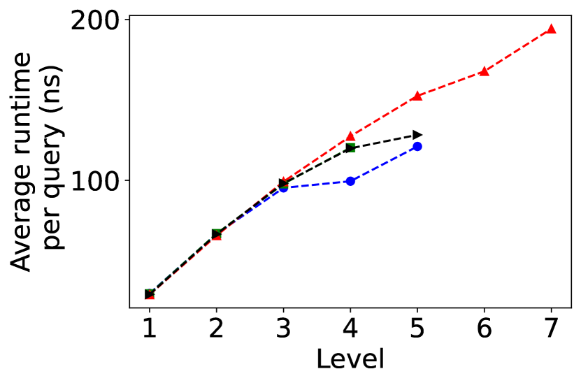
Figure 1: Query time at each level of the LIPP index for four real datasets, each with 200 million keys.

In this paper, we approach the problem from an alternate perspective – we adjust the CDF such that it becomes easier to be approximated by the indexing functions, to achieve lower approximation errors and higher query efficiency.

Our core idea is to add virtual points to “smooth” the CDF of a dataset to be indexed. Take Fig. 2(a) as an example, where each black dot represents a data point (i.e., its search key). Approximating the CDF of the dataset with a linear indexing function can result in a large approximation error (and hence high search costs at query time) for keys $k_{1}$ and $k_{2}$. We sum up the squared prediction error of every point:

$$\mathcal{L}_{f}(K)=\sum_{i=1}^{n}\big{(}f(k_{i})-rank(k_{i})\big{)}^{2},$$ (1)

where $K$ denotes the set of keys and $n$ is its size, $k_{i}\in K$ is a key, $rank(k_{i})$ is its rank, and $f(\cdot)$ denotes the indexing function, respectively. We refer to $\mathcal{L}_{f}(K)$ as sum of squared errors (SSE). In this case, $\mathcal{L}_{f}(K)=8.33$ – a large value of $\mathcal{L}_{f}(K)$ suggests worse prediction accuracy using $f$ for search key mapping and hence higher query times.

As Fig. 2(b) shows, we add a set of virtual points $V=\{k_{v1},k_{v2},\ldots,k_{v5}\}$ represented by the red hollow dots. Here, we assume a smoothing budget of $0.5n=5$, i.e., 5 virtual points are allowed. Now the original data points are spread out, and the CDF of the (original and virtual) points is closer to a straight line. We refit the points with a new index function $f^{\prime}$, with the SSE $\mathcal{L}_{f^{\prime}}(K)$ being reduced to 2.05 (SSE with the new virtual points, $\mathcal{L}_{f^{\prime}}(K\cup V)$ = 2.29).

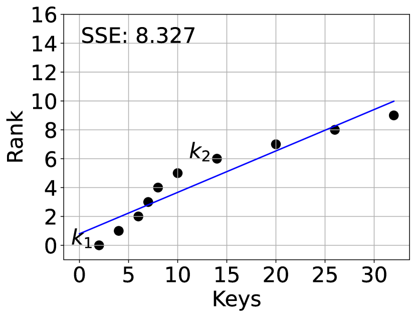
(a) Before smoothing

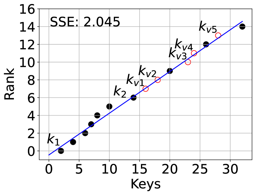
(b) After smoothing

Figure 2: Indexing data points (keys) with CDF smoothing.

We show that, given a smoothing budget that constraints the additional space costs, finding the optimal placement of the virtual points to minimise the SSE $\mathcal{L}_{f^{\prime}}(K)$ is NP-hard. We then consider approximation solutions for two generic scenarios: (1) smoothing the CDF for index learning with a single indexing function and (2) smoothing the CDF for a hierarchy of indexing functions, which is a common structure of existing learned indexes. We focus on linear index functions for their high efficiency, although the idea of CDF smoothing extends to more complex (e.g., quadratic) functions naturally.

We propose an algorithm named CDF smoothing via virtual points (CSV) to smooth the CDF for optimising hierarchical learned indexes, with the aim to reduce the overall height of the structures as well as the prediction errors of each indexing function, and hence the query costs. This is performed by collecting sub-trees of the hierarchical structure and smoothing the CDF of the keys in them by inserting virtual points. As a result, the keys could now be placed into a single node due to the higher learnability, provided it surpasses a cost model threshold value. Here, the cost model is used to balance the reduction in query traversal time and the potential increase in the leaf-node search time due to the increase of keys in a node.

It is important to note that our aim is not to propose yet another learned index but rather a technique that can be integrated with existing or emerging hierarchical learned indexes to optimise their query efficiency with controllable extra space. To show the applicability of our CSV algorithm, we integrate it with three recent learned indexes ALEX [2], LIPP [4], and SALI [14], which are the state-of-the-art (SOTA). Experimental results show that, powered by CSV, these learned indexes have a consistent improvement in the query efficiency, with limited overheads in the storage space.

To summarize, this paper makes the following contributions:

• We propose a key space transformation technique using CDF smoothing via inserting virtual points to enhance the index learnability.

• We propose an efficient algorithm named CSV to integrate the CDF smoothing technique with hierarchical learned indexes to improve the query performance of such indexes, with a controllable space overhead.

• We integrate CSV with three learned indexes ALEX, LIPP, and SALI, and we conduct experiments with four real datasets. The experimental results show that the learned indexes powered by CSV manage to promote up to 60% of the keys in lower levels to upper levels, resulting in up to 34% improvement of their query time.

II Related Work

We first review learned indexes in general. Then, we discuss the gapped array technique used to accommodate insertions and their relevance to our work. Afterwards, we focus on studies addressing complex distributions, which share a similar goal with us. We also cover a technical called the poisoning attacks, which motivates our CDF smoothing technique.

II-A Learned Indexes

Learned indexes are a trending topic in the database community [2, 3, 4, 5, 9, 1, 18, 15, 16]. Their key insight is to treat indexes as functions that map a search key to the storage position of the corresponding data object, which can be learned using machine learning models. A common approach is to layout the data objects by ascending order of their search keys, such that the indexing functions are effectively (approximations of) CDFs of the search keys.

To index large datasets, multiple indexing functions are used, typically organized in a hierarchical structure like a B-tree. The lookup performance of such a structure is then dominated by two steps: (1) the traversal time to find the leaf-node (every node corresponds to an indexing function) indexing the search key, and (2) the search time within the selected leaf-node (leaf-node search time hereafter to distinguish from the traversal time) to locate the target data object, as the indexing functions have prediction errors and may not produce the exact storage position of the search target [21, 22].

It is a challenge to balance the query costs from these two steps mentioned above. While a deeper structure with more indexing functions may fit the data distribution better and have lower leaf-node search times, it may also have higher traversal times and larger index size [23, 24]. Some studies impose a maximum error bound on the indexing functions to reduce the leaf-node search times [20, 3], also at the cost of more indexing functions. Another approach is to use more complex indexing functions (as opposed to linear ones) [1, 13, 18], e.g., splines, which could better fit the CDFs. The issue with this approach is the higher function inference time, and hence higher query and insertion times [21].

These studies design structures and indexing functions to better fit the data distribution. We address the challenge from an alternate perspective, i.e., we adjust the data distribution such that it is easier to be fit by the indexing functions.

II-B Learned Indexes with Gapped Arrays

Several learned indexes [2, 4, 15] leave gaps in their storage structure (i.e., gapped arrays). While their purpose is to accommodate data insertions, a side effect is changing the data distribution, which is what we do. A core difference to note is that, they have not considered minimising the indexes’ model prediction errors when adding gaps, while we do.

II-C Learned Indexes Addressing Complex Data Distributions

To better index CDFs of complex data distributions, there are two common approaches. One is to use more complex functions such as splines and piece-wise linear regression models [3, 18]. The other is to use better data partitioning strategies for easier CDF learning over each partition, such as by CARMI [25] and EWALI [26]. Another study, LER [27], uses logarithmic error-based loss functions (instead of the more commonly used least squared error-based) to improve the learning of index models that better fit the CDF.

A latest development, SALI [14], identifies the most frequently accessed nodes via probability models given a query workload. The corresponding sub-trees are flattened by using a segmentation approach, similar to the PGM index [3], to reduce the traversal time within these sub-trees. However, this leads to an additional search step for query processing, as we need to find the correct node from the flattened structure.

A couple of studies [23, 28] transform the input key set into a more uniform distribution to improve the CDF learnability. The NFL index [23] transforms the key distribution using a numerical normalizing flow that transforms a latent distribution to a new distribution via generative models. The distribution transformation introduces overheads, while queries also need to be transformed to use the index. Further, the transformation may increase the tail conflict degree for certain distributions, making it unsuitable in those instances. The gap insertion [28] technique inserts gaps between the keys (i.e., storage positions of the corresponding data objects) to straighten the CDF of the keys, thereby improving its learnability. However, this is performed by manipulating the rank of each key, and as a result, multiple keys could be given the same position. An extra array is used to house such conflicting keys, which in turn introduces search overheads to locate the correct key at query time. Further, this method leads to a heavy storage space increase of up to 87%. Neither NFL nor gap insertion considers future insertions at construction time. They are less resilient against data updates.

II-D Poisoning Cumulative Distribution Functions

Our idea of adjusting data distribution to fit the indexing functions is rooted from data poisoning – a process of manipulating the training data to change the results from a predictive model [29]. Data poisoning has been introduced into learned indexes to poison the indexing functions and negatively impact their capability to approximate the CDFs [29]. The main goal of this process is to identify new points to include into the original key set that would cause the maximum increase to the loss function value (i.e., the SSE).

Motivated by the poisoning technique, we propose a technique that smooths the data distribution by adding virtual points (i.e., new keys), to obtain CDFs that are easier to be approximated by indexing functions (models), hence leading to a structure with higher query efficiency. Since the models are built with virtual points that can be used to host data insertions, a side benefit of our structure is that it is more resilient against data insertions. Table I highlights the key difference between our technique (CSV), NFL and gap insertion.

TABLE I: Comparison with Existing Works

	CSV	NFL [23]	Gap insertion [28]
No extra transformation at query time	✓	✗	✓
Low storage overhead	✓	✓	✗
Integrable into other learned indexes	✓	✓	✗
Robust across different distributions	✓	✗	✓

III Preliminaries

Problem statement. Consider a dataset $D$ of $n$ data records, where each record is associated with a one-dimensional value as its index key. Let $K$ be the list of all index keys associated with $D$, sorted in ascending order.

Suppose that the index keys have been partitioned and indexed by a set $\mathcal{F}$ of $m$ indexing functions. Each indexing function $f_{i}\in\mathcal{F}$ has some prediction error for a key $k\in K_{i}$ indexed by it. Here, $K_{i}\subset K$ refers to the subset of keys indexed by $f_{i}$. The prediction error refers to the squared difference between the predicted index position $f_{i}(k)$ and the rank of $k$ in $K$, i.e., $rank(k)$.

Let $\mathcal{L}_{\mathcal{F}}$ be the total sum of squared errors of all indexing functions in $\mathcal{F}$:

$$\mathcal{L}_{\mathcal{F}}(K)=\sum_{i=1}^{m}\sum_{k\in K_{i}}\big{(}f_{i}(k)-rank(k)\big{)}^{2}.$$ (2)

The sum of squared errors (SSE) is chosen as it is one of the most commonly used metric to represent loss in the existing studies of learned indexes.

Our aim is to insert values (virtual points) into $K$ while keeping it sorted, i.e., to smooth the CDF of $K$, such that the total SSE is minimised.

A naive optimal smoothing scheme is to insert as many virtual points as needed such that every point $k\in K_{i}$ lies at the $f_{i}(k)$-th position (i.e., $rank(k)=f_{i}(k)$) in the list (assuming unique integer keys). This way, the total prediction error becomes zero after smoothing. In reality, this smoothing scheme is not always feasible, due to the non-uniqueness of the keys in $K$ and the potentially high space cost.

We consider a “smoothing budget” $\lambda$, i.e., the number of virtual points allowed to be inserted, such that total SSE is minimised given the constraint of $\lambda$.

Definition 1

[Learned index smoothing] Given a list of index keys $K$ sorted in ascending order and partitioned into $m$ segments, each of which is indexed by an indexing function $f_{i}\in\mathcal{F}$, the learned index smoothing problem aims to insert a set $V$ ($|V|\leq\lambda$) of virtual points into $K$ while keeping $K$ in order, such that the total SSE is minimised.

We consider linear indexing functions as they are used in most existing learned indexes. We assume $\lambda=\alpha\cdot n$ where the smoothing threshold $\alpha$ is in $(0,1)$, to retain a linear space overhead. To simplify the discussion, we use integer index keys, while our techniques also apply to real number index keys when they can be scaled up to become integers.

NP-hardness analysis. Solving the exact CDF smoothing problem is NP-hard because it can be reduced from the min-Knapsack problem, which is a known NP-hard problem. The min-Knapsack problem considers a given set of items $S$ and a target weight $t$. Each item $s\in S$ is associated with a cost $c_{s}$ and a weight $w_{s}$. The objective is determining the subset $A\subseteq S$ that minimises the total cost of the items in $A$ while the total weight of the items is equal to or greater than $t$.

Our learned index smoothing problem considers a key set $K=\{k_{1},k_{2},\ldots,k_{n}\}$ of size $n$. We aim to find a subset $V$ (virtual points, $k_{vi}$) of at most size $\lambda$ from a candidate set $C$ that would minimise the loss function value $\mathcal{L}$. Naively, the set $C$ can be formed by considering $\lambda$ virtual point candidates between every two adjacent keys in $K$, i.e., $|C|\leq\lambda\cdot(n-1)$.

To reduce the NP-hard min-Knapsack to our problem, we set the weight of every item to 1. Further, the target weight value $t$ should be set to 0, as it is possible to have no virtual points to reduce the loss value. To enforce the smoothing budget, we add an upper limit $\lambda$ to the summation of the weights, which would not change the NP-hardness of this min-Knapsack problem. Now the set $S$ can be mapped to set $C$, and choosing the best virtual point subset $V$ can be mapped to finding the subset $A$ that minimises the loss function in our problem and the objective function in the min-Knapsack problem, respectively. This transformation can be performed in polynomial time, and when our problem is solved, the min-Knapsack problem is solved. As such, our problem is NP-hard.

Due to the difficulties in finding an exact optimal solution for the learned index smoothing problem, next, we consider two reduced versions of the problem and propose highly effective heuristic solutions: (1) smoothing the CDF for the subset of keys $K_{i}$ indexed by an indexing function $f_{i}$ (Section IV); and (2) smoothing the CDFs for all $m$ subsets $K_{i}$ when they are indexed under a hierarchical learned index (Section V).

IV CDF Smoothing for a Single Linear Model

We start with a single indexing function over a segment of keys $K_{i}$. The optimisation goal can be written as:

$$\text{argmin}_{V_{i},\theta}\mathcal{L}_{f_{\theta}}(K_{i}\cup V_{i}),\quad s.t.|V_{i}|\leq\lambda$$ (3)

Here, $V_{i}$ represents the set of virtual keys added to the key set, and $\theta$ denotes the parameters used to define the refitted indexing function $f$ over $K_{i}\cup V_{i}$ – recall that we refit the indexing function after virtual point insertions. We include $V_{i}$ in the calculation to fit also the virtual points, such that the virtual points can be used to accommodate future insertions.

Solution overview. To locate the best virtual point to be inserted, we need to know the new SSE $\mathcal{L}_{f_{\theta}}(K_{i}\cup V_{i})$ after inserting each potential virtual point. To calculate the SSE for just one virtual point, it takes $O(n)$ time where $n$ is the size of $K_{i}$. Suppose that there are $p$ possible values (and hence $p$ candidate insertion positions) for the virtual point. Then, $O(n\cdot p)$ time is needed to find the best value for the insertion.

As both $n$ and $p$ can be large for real datasets, we propose an efficient solution with three main steps: (1) We calculate the loss function value of each candidate insertion position (that is, what will be the error if a point is inserted at that position; Section IV-A). (2) Based on the calculated loss function values and their first partial derivatives, we filter the candidate positions (Section IV-B). (3) From the remaining candidates, we present an efficient algorithm to find the best subset of virtual points of size $\lambda$ (Section IV-C).

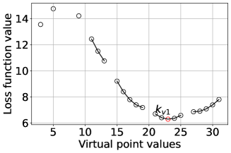
Figure 3: Prediction errors (SSE) corresponding to different insertion positions for a virtual point.

To reduce the search space for the virtual point insertions, we bound it between $(\min\{K_{i}\},\max\{K_{i}\})$. This is because any virtual points added prior to $\min\{K_{i}\}$ would cause all keys’ ranks to increase at the same time, while adding virtual keys after $\max\{K_{i}\}$ would not impact any key’s rank. As such, neither would help achieve a better-fitted indexing function. We also skip the index keys already in $K_{i}$, such that our solution can be compatible with learned indexes that do not support duplicate keys [21]. These skipped keys break the candidate virtual point values (i.e., insertion positions) into segments (i.e., sub-sequences) as shown in Fig. 3, which corresponds to the keys in Fig. 2(a). Each of such sub-sequences are convex, as shown in [29]. In Fig. 3, every hollow dot represents a candidate virtual point. Its $y$-value represents the new loss value (i.e., SSE) when the virtual point is included into the key set. Adjacent hollow dots are linked together, forming a segment of virtual point values. For example, the segment formed by 21 to 25 in the figure is between index keys 20 and 26. Inserting a virtual point with value 23 leads to the smallest SSE as shown in the figure.

IV-A Inserting One Virtual Point

We first optimise the loss calculation for each candidate virtual point. It is computationally expensive to calculate the SSE for each candidate virtual point due to the size of the original key set. We present the following modified equations for the refitting of the index function, such that the included virtual point is separated from the values in the original key set, making the equations dependent only on the inserted virtual point. This way, we enable a single total SSE calculation for the original key, which is then reused to reduce the computational costs when computing the total SSE for the candidate virtual points.

Equations 4 and 5 below compute the new coefficients ($w$ and $b$) for the indexing function $f_{i}$ (shown in Fig. 2(b)).

$$w=\frac{(\sum_{i=1}^{n}k_{i}y_{i}+k_{v}y_{v})-(n+1)\bar{k_{v}}\bar{y_{v}}}{(\sum_{i=1}^{n}k_{i}^{2}+k_{v}^{2})-(n+1)\bar{k_{v}^{2}}},$$ (4)

$$b=\bar{y_{v}}-w\bar{k_{v}}.$$ (5)

Here, the new virtual point is given by $k_{v}$, and the rank of key $k_{i}$ is given by $y_{i}$ (assuming that the ranks start from 0). Further, $\bar{k_{v}}$ and $\bar{y_{v}}$ are the mean of the key set and the rank set after inserting the virtual point $(k_{v},y_{v})$, respectively (i.e., the means of the keys and ranks in Fig. 2(b)). They can be computed by Equations 6 and 7 as follows:

$$\bar{k_{v}}=\frac{\sum_{i=1}^{n}k_{i}+k_{v}}{n+1},$$ (6)

$$\bar{y_{v}}=\frac{\sum_{i=1}^{n}y_{i}+n}{n+1}.$$ (7)

Equations 8 to 11 are devised for the efficient computation of the terms in Equations 4 and 5.

$$\sum_{i=1}^{n}y_{i}=\sum_{i=1}^{n}y_{original_{i}}+n-y_{v},$$ (8)

$$\bar{y}=\frac{\sum_{i=1}^{n}y_{i}}{n},$$ (9)

$$\bar{k}=\frac{\sum_{i=1}^{n}k_{i}}{n},$$ (10)

$$\sum_{i=1}^{n}k_{i}y_{i}=\sum_{i=1}^{n}k_{i}y_{original_{i}}+\sum_{i=y_{v}}^{n}k_{i}.$$ (11)

Here, $\bar{k}$ and $\bar{y}$ are the mean of the key set and the rank set before inserting the virtual point $(k_{v},y_{v})$, respectively (i.e., the means of the keys and ranks in Fig. 2(a)); $y_{original_{i}}$ refers to the rank of key $k_{i}$ prior to inserting the virtual point.

The prediction error function, where the virtual point is separated, is given in Equation 12. This rewritten function enables the values for any candidate virtual point to be calculated efficiently by simply adding the error of the candidate virtual point to the already calculated errors of the original key set. In the case of inserting $\lambda$ virtual points, after inserting one virtual point $(k_{v1},y_{v1})$ and then to find the next virtual point $(k_{v2},y_{v2})$, errors of the original key set will be adjusted to include the error of $(k_{v1},y_{v1})$. As a result, the total SSE values for the candidate virtual points for $(k_{v2},y_{v2})$ can also be easily calculated.

$$\begin{split}\mathcal{L}_{i}(\{K_{i}\cup V_{i}\})=w^{2}\sum_{i=1}^{n}k_{i}^{2}+2wbn\bar{k}\\ -2w\sum_{i=1}^{n}k_{i}y_{i}+nb^{2}-2nb\bar{y}\\ +\sum_{i=1}^{n}y_{original_{i}}^{2}+n^{2}-y_{v}^{2}+(w{k_{v}}+b-y_{v})^{2}\end{split}$$ (12)

IV-B Filtering Virtual Point Candidates

In this subsection, we present an efficient approach to find the candidate virtual points that will reduce the loss function (i.e., total SSE) using the derivative of the loss function, thus providing a much smaller set of candidate virtual points. This step is important because while using the equations above helps improve the efficiency of processing one candidate virtual point, the number of candidate virtual points to be processed can still be large, causing substantial overheads.

Fig. 4 plots the partial derivative of the total SSE with respect to a candidate virtual point. The sub-sequences (depicted as lines or dots) that cross the zero $x$-axis would imply that there is a minimum point within the sub-sequence. Otherwise, the minimum point would be in one of the endpoints of the sub-sequence of candidate virtual points. This observation is exploited to streamline the selection of candidate virtual points, i.e., to select the best virtual point from each sub-sequence.

Similar to the computation of the total SSE, the partial derivative of total SSE with respect to candidate virtual point $k_{v}$ can also be computed by Equation 13:

$$\begin{split}{\mathcal{L}_{i}(\{K_{i}\cup V_{i}\})}^{\prime}=2({w}^{\prime}(w\sum_{i=1}^{n}k_{i}^{2}+nb\bar{k}-\sum_{i=1}^{n}k_{i}y_{i})+\\ n{b}^{\prime}(w\bar{k}+b-\bar{y})+(wk_{v}+b-y_{v})({w}^{\prime}k_{v}+w+{b}^{\prime})).\end{split}$$ (13)

Here, $w^{\prime}$ and $b^{\prime}$ refer to the partial derivative of the slope $w$ and the intercept $b$ with respect to the candidate virtual point $k_{v}$. They can be computed by Equations 14 and 15, respectively.

$${w}^{\prime}=\frac{A(n(y_{v}-\bar{y}))-B(2n(k_{v}-\bar{k}))}{A^{2}},$$ (14)

$${b}^{\prime}=-\frac{(w+(n+1)\bar{k_{v}}{w}^{\prime})}{n+1},$$ (15)

$$A=(n+1)(\sum_{i=1}^{n}k_{i}^{2}+k_{v}^{2})-((n+1)\bar{k_{v}})^{2},$$ (16)

$$B=(n+1)(\sum_{i=1}^{n}k_{i}y_{i}+k_{v}y_{v})-(n+1)^{2}\bar{k_{v}}\bar{y_{v}}.$$ (17)

Here, $A$ and $B$ are intermediary for computing the partial derivatives.

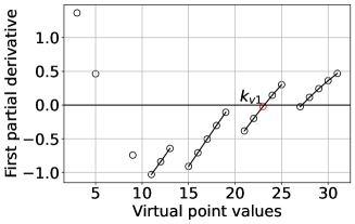
Figure 4: First partial derivative of the loss function with respect to different insertion positions for a virtual point

IV-C Inserting $\lambda$ Virtual Points

After filtering the candidate virtual points, among the remaining ones, we present an efficient algorithm to find the best subset of candidate virtual points of size $\lambda$.

When there are $\lambda$ virtual points to insert, the optimal solution would require computing the total SSE for every size-$\lambda$ subset of the candidate virtual points in the range of $[\min\{K_{i}\},\max\{K_{i}\}]$. If there are $p$ possible insertion positions for the virtual points, the time complexity will be $O(^{p}C_{\lambda}\cdot n\cdot p)$, where ${}^{p}C_{\lambda}$ is the combination of every size-$\lambda$ subset from $p$. As this will be prohibitively expensive for a large dataset, we propose a greedy algorithms and insert individual virtual points iteratively.

The core idea is to identify the virtual point that would minimise the total SSE for each sub-sequence (i.e., local minima for the sub-sequences) and select the one that reduces the total SSE the most (i.e., global minimum). This process needs to be performed $\lambda$ times. The algorithm for CDF smoothing by inserting $\lambda$ virtual points is summarized in Algorithm 1 and described below.

Algorithm 1 CDF_smoothing

1:Key set: $K$, loss function with new virtual point: $\mathcal{L}(k_{v})$, smoothing threshold: $\alpha$

2:$U$, $C$, $V=[]$

3:$G=[]$, $M=[]$ $\triangleright$ Arrays of point pairs

4:$\mathcal{L}^{\prime}(k_{v})=\frac{\partial L(k_{v})}{\partial k_{v}}$, $\lambda=\alpha\cdot K.size$, $\mathcal{L}_{previous}=\mathcal{L}(\varnothing)$

5:Find the endpoint pairs, $E$, for each sub-sequence

6:while $V.size<\lambda$ do

7:    for $i$ from 1 to $E.size$ do $\triangleright$ Separate sub-sequences

8:         if $E[i].second$ - $E[i].first\leq 1$ then

9:             Append $E[i].first$ and $E[i].second$ to $C$

10:         else$\triangleright$ There are more than 2 points

11:             Append $E[i].first$ to $G.first$ and $E[i].second$ to $G.second$

12:         end if

13:    end for

14:    for $i$ from 1 to $G.size$ do $\triangleright$ Calculate the partial derivatives

15:         if $\mathcal{L}^{\prime}(G[i].first)\cdot\mathcal{L}^{\prime}(G[i].second)<$ 0 then

16:             Append $G[i].first$ to $M.first$ and $G[i].second$ to $M.second$

17:         else

18:             Append $G[i].first$ and $G[i].second$ to $C$

19:         end if

20:    end for

21:    for $i$ from 1 to $M.size$ do $\triangleright$ Calculate minimum point

22:         Append $minimum\_point(M[i].first$, $M[i].second)$ to $C$

23:    end for

24:    for $i$ from 1 to $C.size$ do $\triangleright$ Calculate loss value

25:         $U[i]$ = $\mathcal{L}(C[i])$

26:    end for

27:    Find index $i$ of minimum $\mathcal{L}$

28:    if $\mathcal{L}_{previous}\leq U[i]$ then

29:         break

30:    end if

31:    Append $C[i]$ to $V$, Append $C[i]$ to $K$, $\mathcal{L}_{previous}=U[i]$

32:end while

33:return C

The algorithm takes as input a key set $K$ (we drop the subscript $i$ from $K_{i}$ to simplify the notation) of size $n$ and a smoothing threshold $\alpha$ (or a smoothing budget $\lambda$ can also be directly provided ). We use $G$ to denote a set that stores the potential sub-sequences, where there can be a candidate virtual point within the sub-sequences with a local minima of the total SSE. The candidate virtual points contributing the local minima are stored in an array $M$, while $C$ stores set of candidate keys for the virtual points. We use $U$ to hold the total SSE value for each candidate virtual point and Vector $V$ to store the final optimal virtual points.

First, the algorithm identifies the sub-sequences of candidate virtual points that could have their minimal total SSE values at the endpoints or in the middle of the sequence. This is shown in Lines 4 to 12. If there are more than two points in a sub-sequence, the candidate virtual point with the minimal total SSE value can be within that sub-sequence. As such, the two endpoints of the sub-sequence are saved in array $G$ for calculating the partial derivatives.

Afterwards, in Lines 13 to 22, the partial derivative of the total SSE with respect to the candidate virtual points is calculated for all point pairs in $G$ using the equations derived above. If the signs of the partial derivatives corresponding to the two endpoints of a sub-sequence are different (i.e., on opposite sides of the $x$-axis), the two endpoints will be added to array $M$ for calculating the minimum point. As shown in Fig. 4, for the sub-sequences that contain candidate virtual points with minimal total SSE values, the partial derivatives of the end points will appear on the two sides of the $x$-axis. These minimal points are added to array $C$ after they are calculated. If the partial derivatives of the two endpoints are on the same side of the $x$-axis, the minima is at one of the endpoints, as such the two end points are added to $C$.

Finally, Lines 23 to 31 compute the total SSE for each candidate virtual point in $C$ and select the point with the minimum total SSE, as long as the new total SSE is smaller than the existing total SSE obtained so far over $K$ and any previously inserted virtual points. This process is repeated until at most $\lambda$ virtual points are inserted, or when the total SSE is not reduced any further. When the algorithm terminates, the final virtual points in $V$ are returned.

Complexity analysis. Our proposed CDF smoothing algorithm reduces the computation of the total SSE values over $K$ to just once, which takes $O(n)$ time. This process is repeated to find $\lambda$ optimal candidate virtual points. However, there is no need to recalculate the loss function value after adding a virtual point, as we could treat the key set with the previous virtual point inserted as the new original or base key set for a constant time calculation. Thereby, giving a time complexity of $O(\lambda+n)$.

V CDF Smoothing for Hierarchical Indexes

In this section, we present the CDF smoothing to a hierarchical learned index to improve the performance of queried keys. A direct application to individual nodes would help reduce leaf-node search time by improving the learnability of the models but fail to address traversal time. Therefore, a method for addressing both traversal and leaf-node search is required. As such we present CSV to smooth segments of the CDF for different sub-trees in the hierarchical structure of a learned index in order to merge and reduce the overall structure height. A major challenge is the balancing between the improvement of traversal time due to the reduction of the index height and the increase in leaf-node search time due to more keys being merged into single nodes. To address this, we present a cost model that takes both of these factors into consideration.

The core idea is to start from the bottom most level of the index that contain parent nodes of leaf-nodes and select those nodes. Then for each of these parents nodes, the keys in the node and its child nodes are collected, which are then subjected to smoothing using Algorithm 1. If the minimum cost threshold is satisfied (more details below), then the sub-tree and the node are reconstructed to merge the collected nodes. The merging is performed by creating a new leaf-node in place of the parent node and placing the keys from the collected nodes. By doing so, more keys would be placed in upper level nodes of the index as the indexing functions of these nodes would be improved by the CDF smoothing, but the cost models would limit the number of keys as to not offset the performance gain by the increase in the leaf-node search time. Further details regarding this is given in Section V-1. This process is performed until the root node depicted as level 1 is reached, thus reducing the total prediction error ($L$). For this purpose, unbalanced learned index structures are better suited as it gives the ability to reduce the height of taller branches without affecting the rest.

Algorithm 2 CSV

1:Nodes with sub trees : $Nodes$, smoothing threshold : $\alpha$, cost threshold : $c$

2:$Nodes=[]$

3:$keyset=[]$

4:$keyset\_smooth=[]$

5:$max\_level$ $\leftarrow$ maximum level of index with sub trees

6:$current\_level$ $\leftarrow$ $max\_level$

7:while $current\_level>1$ do

8:    $Nodes\leftarrow$ all nodes with sub trees

9:    for $i$ from 1 to $Nodes.size$ do

10:         $keyset\leftarrow$ collect all keys in the node and its sub tree

11:         $keyset\_smooth\leftarrow$ $CDF\_smoothing(keyset,\alpha)$ $\triangleright$ Using Algorithm 1

12:         if $cost<c$ then

13:             Reconstruct the sub-tree and node with $keyset\_smooth$

14:         end if

15:    end for

16:    $current\_level\leftarrow current\_level-1$

17:end while

The algorithm for an unbalanced learned index structure is given in Algorithm 2 and described below. First the algorithm starting from the maximum level of the index, and identifies all nodes with sub-trees, which is shown in Lines 5-7. Afterwards, as shown in Lines 8-14, each of the node’s and its sub-tree’s keys are collected and subjected to the CDF smoothing. Provided that they meet the minimum cost threshold selected, the node and its sub-tree are reconstructed to promote as many keys to upper levels as possible. This process is iteratively performed in a bottom up manner for other levels of the index.

Complexity analysis. For a key set of size $n$, with a smoothing budget of $\lambda$ and an index structure with $m$ non-leaf nodes, the complexity for the developed algorithm can be calculated as follows. The complexity for $node_{i}$ with $n_{i}$ keys and a smoothing budget of $\lambda_{i}$ is $O(\lambda_{i}+n_{i})$. Similarly, for the $m$ nodes, we would get a complexity of $O(\lambda_{1}+n_{1}+\lambda_{2}+n_{2}+\cdots+\lambda_{m}+n_{m})$. This can be simplified to $O(\lambda+n)$.

V-1 Cost conditions

For indexes that does not contain any searching component such as LIPP and SALI, their loss function values can be taken as the cost conditions. This is because if the new model could hold more keys than before, then it does not have any other component (that is, leaf-node search time) that would negatively affect the performance. However, for the indexes with leaf-node search components like ALEX, there must be a trade-off between the increase of leaf-node search time over the reduction of traversal time. The reason is, introducing new keys into the node would require more time to locate the key. For this purpose, we develop the following cost model, where reconstruction is performed only if the cost is less than a specified threshold value, $c$.

$$\begin{split}cost=search\_constant\times expected\_number\_of\_searches\\ +traversal\_constant\times index\_level\end{split}$$ (18)

To make the implementation hardware independent, the constants can be measured by sampling queries to measure the time spent per leaf-node search for the case of $search\_constant$ and the traversal time spent per level for $traversal\_constant$. The $expected\_number\_of\_searches$ can be calculated via the inbuilt function in ALEX that uses the $log_{2}$ error to estimate it. Considering the cost model depicts the expected query time for the node, the cost threshold, $c$ should be set below 0 to identify an improvement. Setting a further lower value would result in fewer keys being able to be promoted to upper levels but the expected query time improvement will be greater.

V-A Approximation Quality Analysis

The effectiveness of our proposed greedy method of iteratively identifying the $\lambda$ virtual points as opposed to the exhaustive manner of comparing all $\lambda$ subsets, is demonstrated via experimentation in this section.

The key set of 10 keys given in Fig. 2 was subjected to CDF smoothing with a smoothing threshold ($\alpha$) of 0.5 (smoothing budget of 5) via both methods. The results are shown in Table II. Here, the greedy method improves the loss by 72.34%, while the exhaustive method improves it by 74.44%. However, the time taken by the exhaustive method is nearly 3 orders of magnitude more than the greedy method. This results show that the effectiveness of the greedy method is similar to the exhaustive method, and the exhaustive method is impractical to use in real datasets.

TABLE II: Approximation Quality Results

	Exhaustive	CSV	Original
Total SSE	2.118	2.293	8.327
Time (ns)	140,656,167	424,667	N/A

VI Experimental results

Next, we report experimental results. The implementation is based on an existing benchmark [30] for easier comparison of existing techniques. All experiments were run on an Ubuntu 20.04.5 virtual machine with an AMD EPYC 7763 64-Core Processor CPU and 128 GB of RAM.

VI-A Experimental Settings

Competitors. To show the general applicability of our proposed techniques, we integrate CSV with recent learned indexes, including ALEX [2], LIPP [4], and SALI [14] (SOTA). These indexes have reported strong empirical performance, outperforming both traditional indexes like the B⁺-tree and learned ones like the PGM index [3], XIndex [13], and FINEdex [12]. For simplicity, we do not repeat the comparison results with these other indexes.

Datasets. We run experiments with four datasets from two benchmark works [31, 22]: (1) Facebook contains 200 million integer Facebook user IDs [32]; (2) Covid contains 200 million integer tweet IDs randomly sampled from tweets tagged with “Covid-19” [33]; (3) OSM contains 200 million locations randomly sampled from OpenStreetMap and represented as Google S2 [34] cell IDs [35]; and (4) Genome contains 200 million entries of loci pairs in human chromosomes represented as integers [36]. For all datasets, duplicate keys were removed because LIPP and SALI do not support them.

Out of the four datasets, OSM and Genome are considered more difficult for learned indexes [22] (hard datasets), while Facebook and Covid are easier (easy datasets). To illustrate this, the CDF of the full datasets are plotted in Figs. 5(a) to 5(d). All datasets except OSM have almost globally linear CDFs. Zooming in the CDFs shows that there is more variability in the local distribution patterns, as shown in Figs. 5(e) to 5(h) (each showing from the 100 million-th data point to the next thousand data points). Except Covid, all datasets deviate from linear CDFs at local level, especially Genome.

(a) Facebook

(b) Covid

(c) OSM

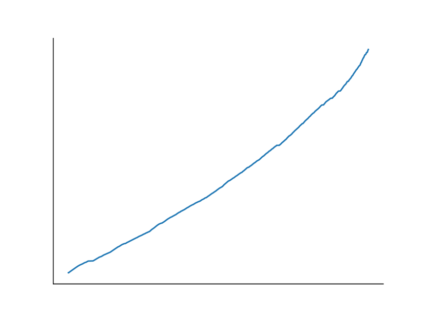
(d) Genome

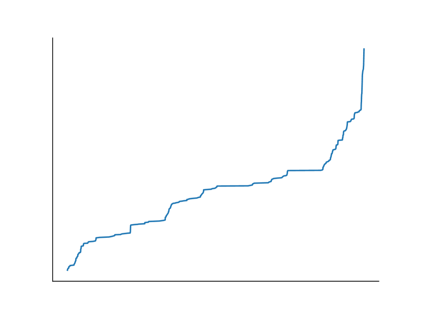
(e) Facebook
(zoomed-in)

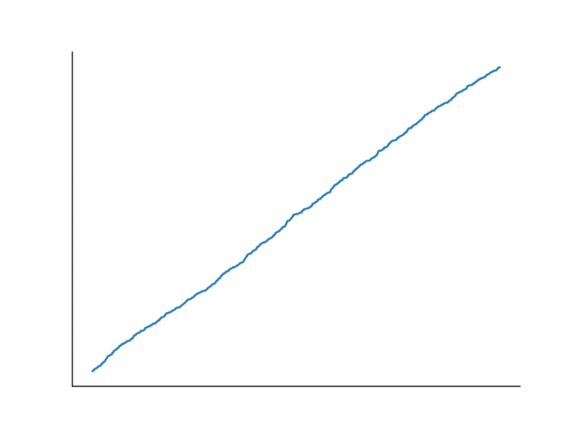
(f) Covid
(zoomed-in)

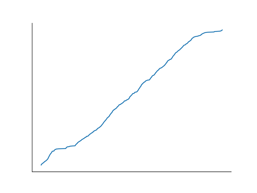
(g) OSM
(zoomed-in)

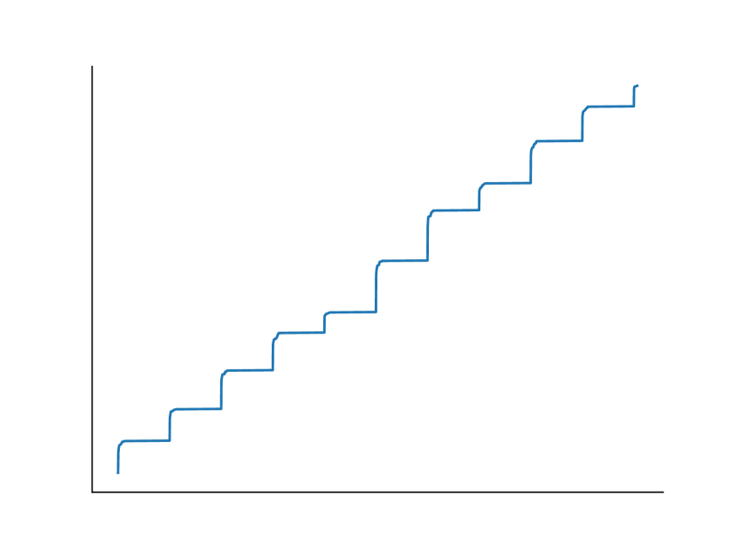
(h) Genome
(zoomed-in)

Figure 5: CDFs of the datasets

Workloads. We use the following two types of workloads:

(1) Read-only workload. The learned indexes ALEX, LIPP, and SALI (same below) are constructed over the full datasets. Afterwards, our CSV algorithm is applied to optimise their structures. Then, the queries (detailed below) are run.

(2) Read-write workload. The learned indexes are constructed and CSV is applied over a random half of each dataset. The other halves are inserted in random insert batches of size $10\%n$. Queries are run after each batch insertion.

We consider three sets of queries over each dataset:

(1) Promoted data. Querying every key that has been promoted to upper levels in the index by our algorithm.

(2) Random. Querying one million keys randomly sampled from each dataset.

(3) Zipfian. Querying one million keys sampled from each dataset using a Zipfian distribution to represent a realistic workload, following a previous work [3].

Parameters. We vary the smoothing threshold, $\alpha$ from 0.05 to 0.8, with a default value of 0.1. To show the scalability of our algorithm by varying the dataset size, the original datasets were down sampled by eliminating every $j$-th key from the sorted datasets in order to remove $n/j$ data points and create smaller datasets of size 12.5 million, 25 million, 50 million, and 100 million, respectively. The default datasets are the original ones with 200 million data points.

For each queried key, the query time was recorded by repeating the query 100 times and taking its average. Since our main goal is to show the query performance gain achievable by our CSV algorithm, we report performance results relative to those produced by the original learned indexes without CSV, in addition to reporting the absolute query time results for random and Zipfian queries.

For LIPP and SALI, they can create nodes that are indexing only a few keys [4]. For these two indexes, CSV is run starting at the second level of the index structures, such that each smoothing step can benefit more points. This is not an issue for ALEX, and CSV is run starting at the bottom level of the structure. Further, since the query times of the keys in the top two levels of the index structures are very close, our CSV algorithm stops at the second level from the top (i.e., the root).

VI-B Results on Read-only Workloads

VI-B1 Impact of Smoothing Threshold

We vary the smoothing threshold from 0.05 to 0.8 to quantify its impact.

Query time (promoted data). The total time saved by CSV, compared to the original index structure are shown in Figures 6a, 6c, and 6e for LIPP, SALI, and ALEX indexes respectively. The general trend is that adding more virtual points (i.e., increasing the smoothing budget, $\alpha$) saves more query times. LIPP and SALI tend to perform quite similarly due to SALI using LIPP as the base index. For LIPP and SALI indexes, the easy to learn datasets (Facebook and Covid) stabilise after a certain number of virtual points are inserted. This is primarily due to the original dataset’s CDF being linear. However, this is not the case for ALEX index primarily due to the leaf-node search term in its query performance.

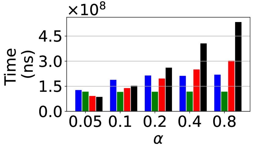
(a) LIPP: Total time saved

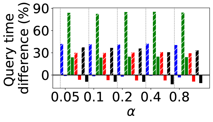
(b) LIPP: Relative query time

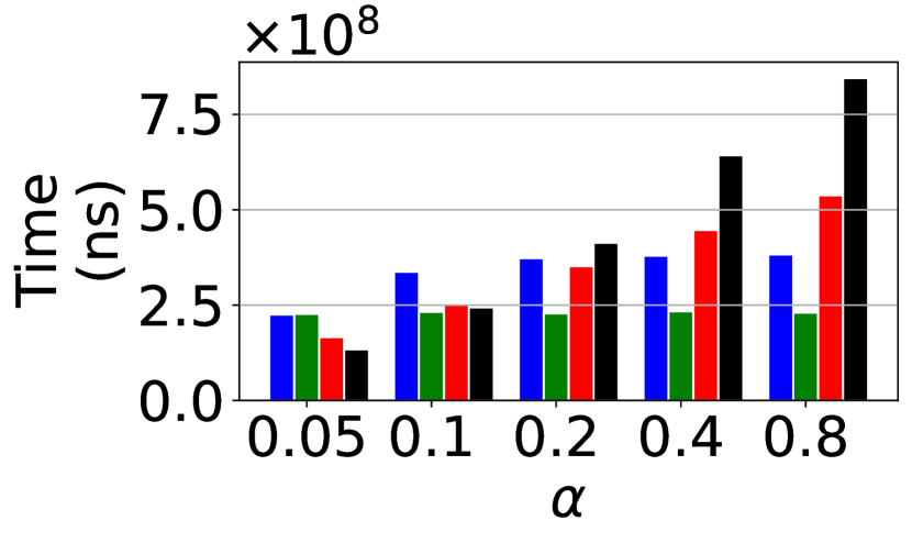
(c) SALI: Total time saved

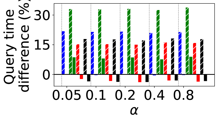
(d) SALI: Relative query time

(e) ALEX: Total time saved

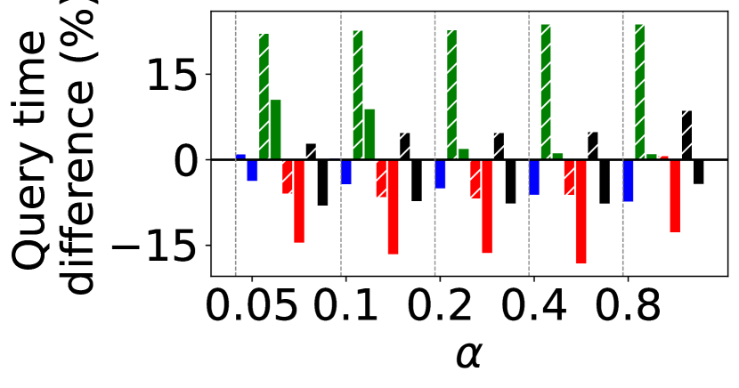
(f) ALEX: Relative query time

Figure 6: Query time vs. smoothing threshold ($\alpha$)

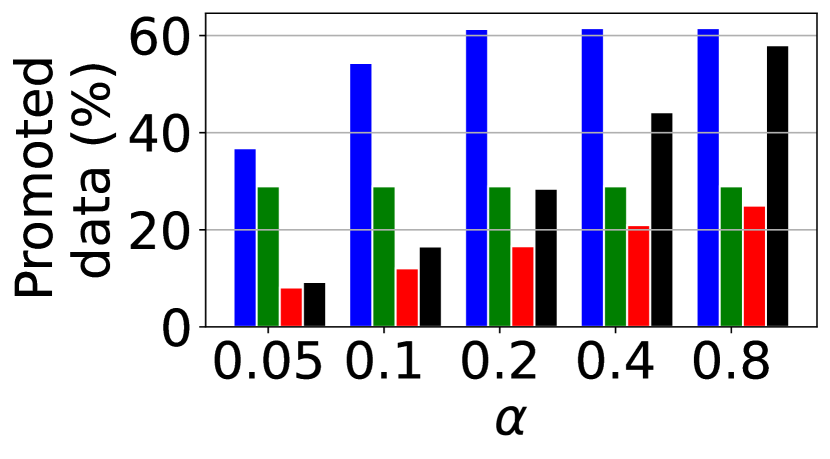
(a) Percentage of
promoted data

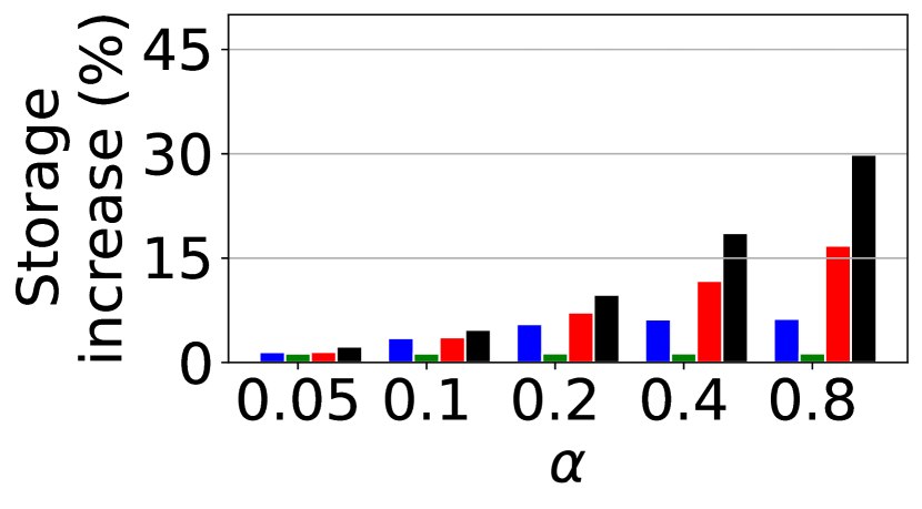
(b) Percentage of storage
space increase

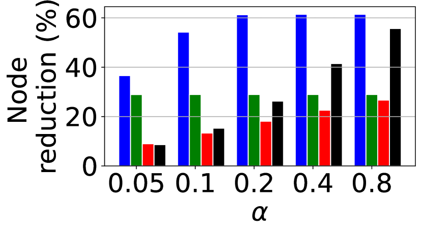
(c) Percentage of index
model reduction

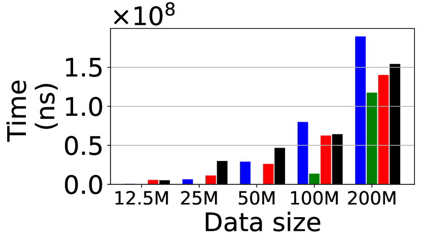
(d) Total time saved vs.
dataset cardinality

Figure 7: (a)-(c): LIPP space cost vs. smoothing threshold, (d): LIPP query time vs. dataset cardinality

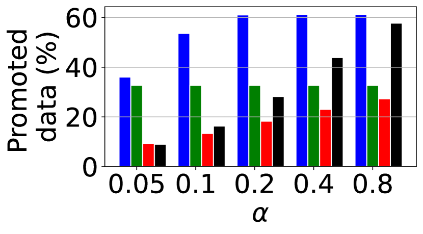
(a) Percentage of
promoted data

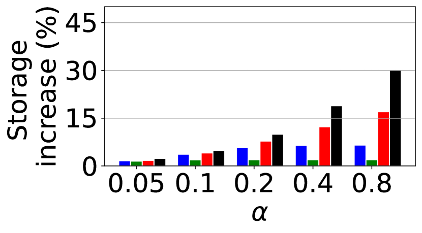
(b) Percentage of storage
space increase

(c) Percentage of index
model reduction

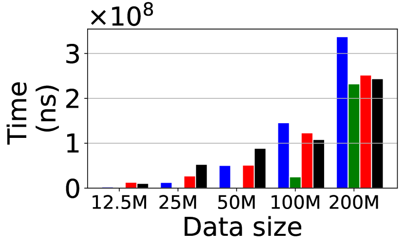
(d) Total time saved vs.
dataset cardinality

Figure 8: (a)-(c): SALI space cost vs. smoothing threshold; (d): SALI query time vs. dataset cardinality

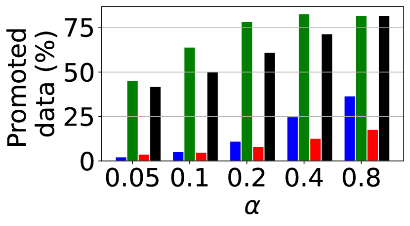
(a) Percentage of
promoted data

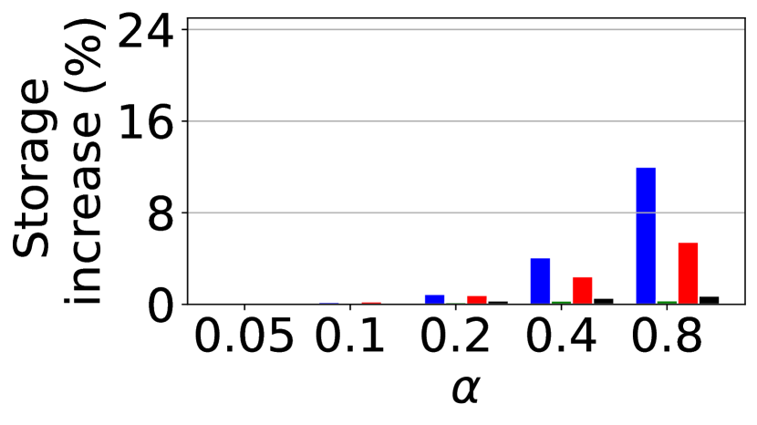
(b) Percentage of storage
space increase

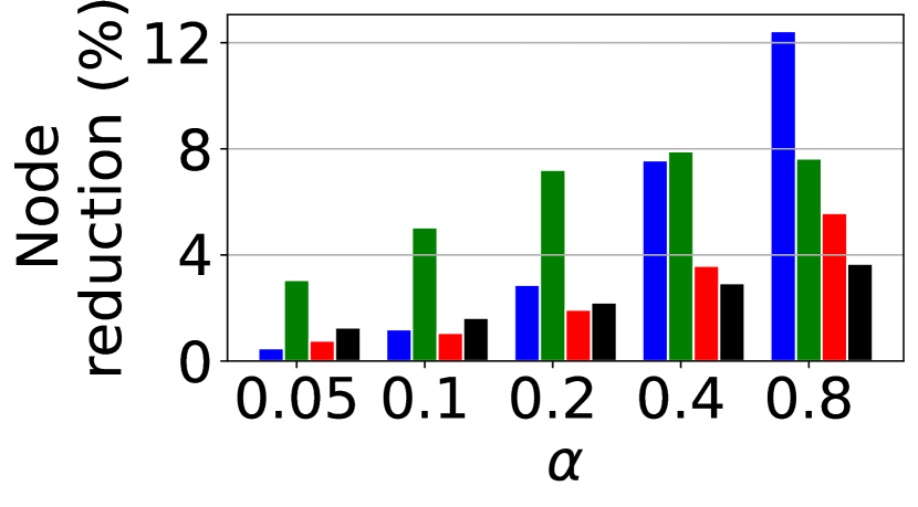
(c) Percentage of index
model reduction

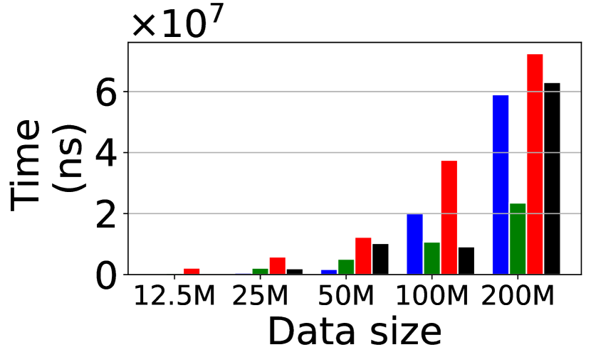
(d) Total time saved vs.
dataset cardinality

Figure 9: (a)-(c): ALEX space cost vs. smoothing threshold; (d): ALEX query time vs. dataset cardinality

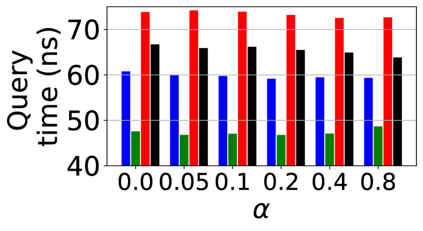
(a) LIPP: Absolute average query time (random)

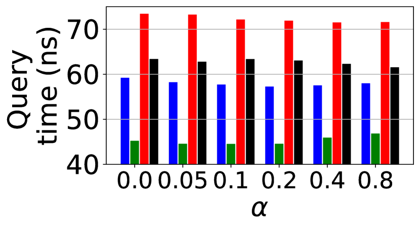
(b) LIPP: Absolute average query time (Zipfian)

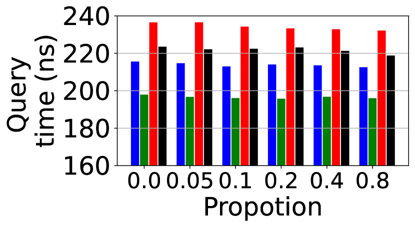
(c) SALI: Absolute average query time (random)

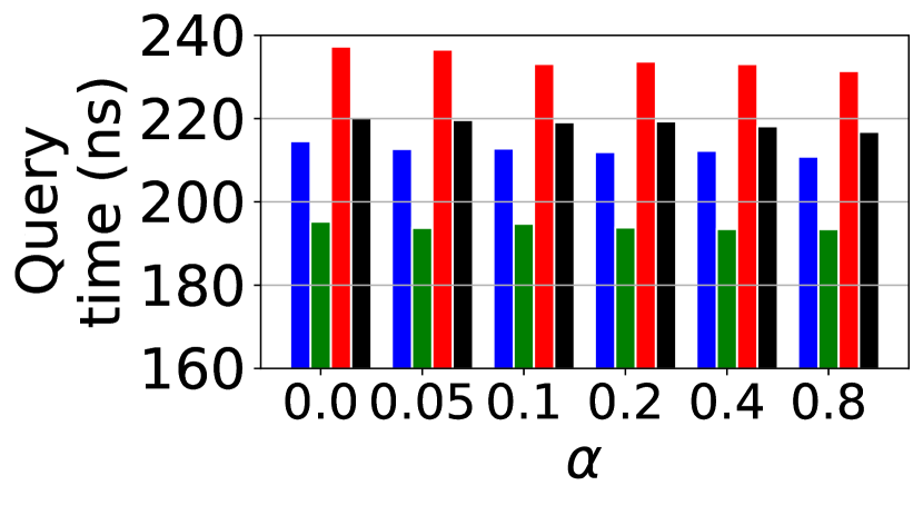
(d) SALI: Absolute average query time (Zipfian)

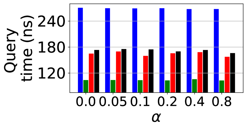
(e) ALEX: Absolute average query time (random)

(f) ALEX: Absolute average query time (Zipfian)

Figure 10: Query time vs. smoothing budget on other query distributions

Figs. 6(b), 6(d), and 6(f) illustrate the query times of the promoted data relative to the average query times of LIPP, SALI, and ALEX, respectively. Here, the line at the $y$-value 0 represents the average query time (that is, the average query time for randomly queried data) before applying CSV (note that, we have also presented the absolute average query time for randomly queried data later in Fig. 10, where $\alpha=0.0$ represent the values for the original indexes). The dashed bars (denoted as ‘Original’) represent the query times as a percentage of the average query time for the promoted data before applying CSV. These figures show that the keys that will be promoted by CSV take a longer query time compared to the average – generally being between 15% to 80% higher than randomly queried data for LIPP and SALI. This is because the keys that will be promoted by CSV are typically at the deeper levels of the index structures that require higher query times.

After applying CSV, the query times of the promoted data as a percentage of the average query time is significantly reduced, They can be even lower than the average query time for larger values of $\alpha$ (shown by the bars below the line with $y$-value 0). As ALEX has an additional leaf-node search step which is not required by LIPP and SALI, the benefit for the promoted data is smaller (since CSV forms larger nodes that could lead to longer leaf-node search times). However, it is important to note that CSV still yields consistent query time improvements for the promoted data (i.e., the bars with solid colours are below the dashed bars of the same colour).

Size of the promoted data. Figs. 7(a), 8(a), and 9(a) show the number of keys promoted to higher levels after applying our CSV algorithm, as a percentage of the total number of keys that can be promoted (i.e., keys at level 3 or below). For the Facebook dataset, CSV can promote around 60% of all possible data to higher levels, while for the Covid dataset, CSV promotes around 30% of the data. For the harder to learn datasets, OSM and Genome, CSV also manages to promote up to 27% and 57% of the data, respectively. The datasets with most promoted data are again different for ALEX, which is consistent with the observations before. Also, while the general patterns are similar to those in the query times saved, higher bars may be observed on some datasets (e.g., Facebook) in these figures than those in the total time saved Figures above. This is because the promoted data is given as a percentage to the keys that can be promoted. Even though OSM and Genome report lower percentages of promoted data, the actual number of promoted data is higher. This is because, they have much higher number of keys in lower levels.

Index size. Due to the addition of virtual points, we expect the storage consumption to increase. This is shown in Figs. 7(b), 8(b), and 9(b). In all cases, less than 31% of additional storage space is required by the CSV-enhanced indexes compared to the original structures, and in most cases, less than 10%. The increase in the space cost is proportional to the smoothing threshold, which is also intuitive.

The storage space increase is balanced out by the removal of unnecessary nodes, whose data is promoted to higher levels. This node reduction follows a similar pattern to the percentage of promoted data, as shown by Figs. 7(c), 8(c) and 9(c). Here, the node reduction is given as a percentage of the nodes that could be removed (nodes at levels 3 or lower of the index structures).

Query time (other query distributions). The average query time for random distribution and Zipfian distribution queries are given in Figs. 10(a), 10(c), and 10(e) and Figs. 10(b), 10(d) and 10(f), respectively. When considering random queries, with the original index performance shown in $\alpha$ value of 0, their performance is slightly improved in most of the cases tested. This can be attributed to the improvements from our smoothing process. The small increase is due to a large number of keys being in higher levels that are not considered for promotion, while the random queries are mostly from those levels. The performance of the queries from the Zipfian distribution shows a similar pattern for the same reason.

Pre-processing time for CSV. The times taken to run CSV to optimise the learned index structures are summarized in Tables III and IV for LIPP and ALEX. As SALI is based on LIPP, where CSV reports a similar performance, we omit the detailed results for brevity.

We see that CSV takes more time to run as the smoothing budget grows, since there are more candidate virtual points to be examined. The algorithm running times vary across different datasets, again because the datasets have different difficulties in index learning. Note that, while the running times of CSV may seem quite large under certain settings, e.g., over 80,000 seconds on OSM for ALEX, however considering CSV can be performed at the same time when the index is constructed prior to deployment, this pre-processing time is amortized by the improvement in query time.

TABLE III: CSV Pre-processing Time (s) for LIPP

	0.05	0.1	0.2	0.4	0.8
Facebook	589	1,194	1,859	2,106	2,228
Covid	304	337	343	337	336
OSM	1,217	2,329	4,495	7,983	13,019
Genome	1,155	2,174	4,616	9,316	15,709

TABLE IV: CSV Pre-processing Time (s) for ALEX

	0.05	0.1	0.2	0.4	0.8
Facebook	247	889	4,123	17,508	48,737
Covid	609	1,423	2,795	4,463	4,955
OSM	988	2,297	9,526	33,097	81,620
Genome	1,356	2,902	6,253	8,854	9,777

VI-B2 Impact of Dataset Cardinality.

To demonstrate the scalability of CSV against the dataset cardinality, we repeat the experiments on datasets of 12.5 million to 200 million data points. Figs. 7(d), 8(d), and 9(d) show the total query times saved by applying CSV. It can be seen that for all datasets, the times saved grow with the dataset cardinality. The rate of improvement on the easier to learn datasets grows faster, since there are not many keys in the deeper levels for these datasets when the dataset cardinality is small. These results confirm the scalability of CSV towards datasets of growing cardinality.

VI-C Results on Read-write Workloads

Due to the similar trends between LIPP and SALI indexes, SALI is omitted from the results below.

Query time (promoted data). Fig. 11 shows the total query times saved by CSV, compared to the original index structures, as more batches of data are inserted. Here, the query times saved are decreasing slightly as more data is inserted for LIPP, because the inserted data have higher chance of colliding with the promoted data as they are now in higher levels, compared to when they are in lower levels as in the original index structure. For ALEX, the trend is quite similar except for on the OSM dataset, where there are two drops after one insertion batch (i.e., $0.1n$ points are inserted) and three insertion batches ((i.e., $0.3n$ points are inserted). This is primarily due to the original index structure’s query times happen to be slightly lower in these two cases.

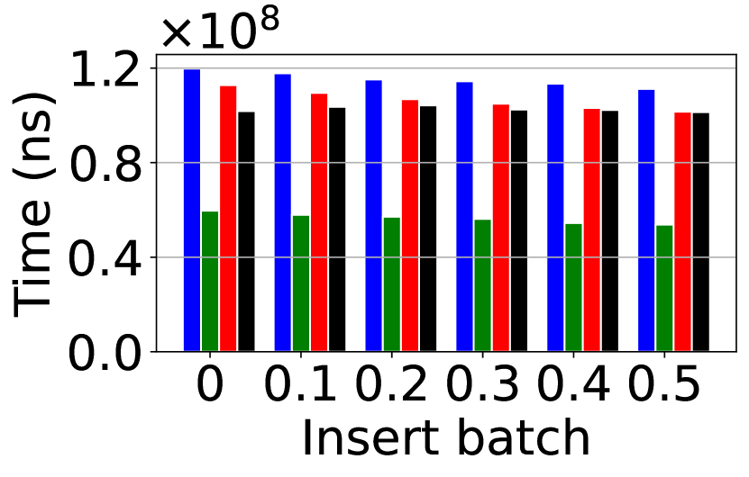
(a) LIPP

(b) ALEX

Figure 11: Total time saved vs. insertion batches (promoted data)

Index size. The index size overhead decreases after each batch of insertions, as shown in Fig. 12. This is because the initial gaps left by the virtual points are gradually filled up by the inserted points, hence improving the overall space utilization. Again, the index size overhead is at or below 10%, emphasizing the space efficiency of CSV.

(a) LIPP

(b) ALEX

Figure 12: Percentage of storage space increase vs. insertion batches

Query time (other distributions). The query times for the random and Zipfian distributions, as shown in Figs. 13 to 16, increase gradually with more data inserted into the index structures, while applying CSV again helps reduce the average query times.

(a) CSV

(b) Original

Figure 13: LIPP: Absolute average query time vs. insertion batches (random)

(a) CSV

(b) Original

Figure 14: ALEX: Absolute average query time vs. insertion batches: original structures (random)

(a) CSV

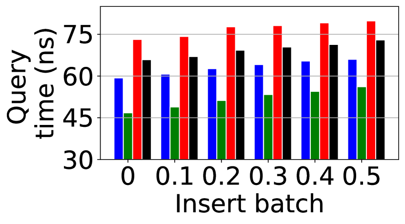
(b) Original

Figure 15: LIPP: Absolute average query time vs. insertion batches (Zipfian)

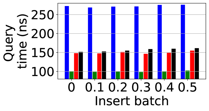
(a) CSV

(b) Original

Figure 16: ALEX: Absolute average query time vs. insertion batches (Zipfian)

Insertion time. Fig. 17 shows the insertion times of the CSV-enhanced indexes relative to those of the original indexes. Using CSV helps improve the insertion times in most cases because the gaps left by the virtual points can be reused for insertions. CSV could also lead to higher insertion times in a few cases. This could be attributed to the fact that there are more keys at the upper levels of the CSV-enhanced indexes which may lead to more collisions with the insertions.

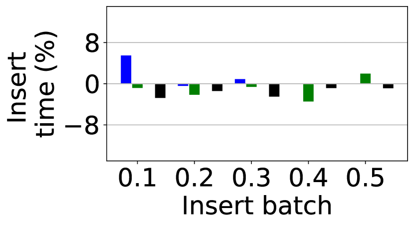
(a) LIPP

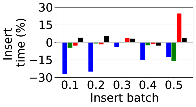
(b) ALEX

Figure 17: Insertion time vs. insertion batches

Robustness to insertion. Figs. 18 to 21 show the data reduced from the CSV as a percentage of the data in the original index structure for each level. It can be seen that fewer keys are inserted to lower levels (negative values) and more keys are promoted to higher levels (positive values). This suggests that the indexing functions created by CSV are more robust to the insertions as there are fewer predictions to the same position, allowing more keys to be placed in the same node. In a very limited number of instances, the CSV-enhanced indexes have more data in some lower levels. This could be attributed to the inserted data having conflicts with the existing keys. However, the maximum such extra keys added in lower levels by CSV is only 22 keys in Fig. 20(a) for level 8.

(a) LIPP

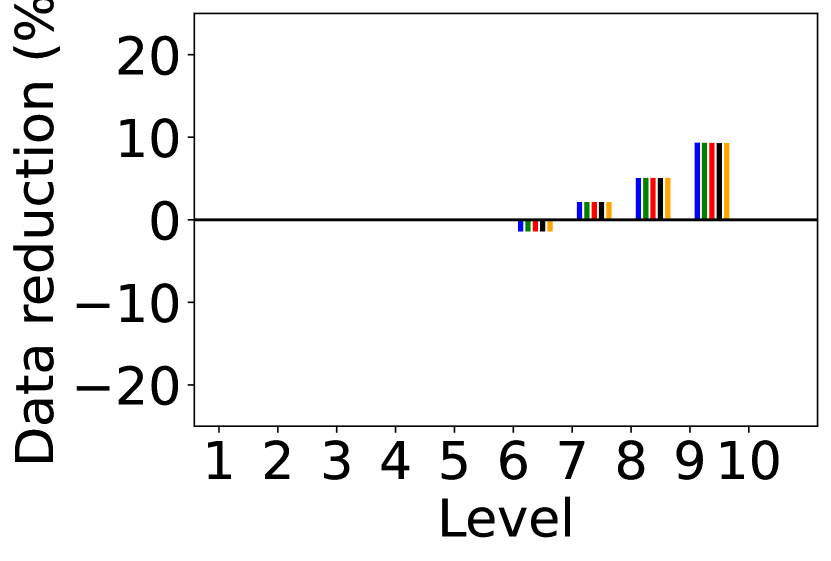
(b) ALEX

Figure 18: Data reduction percentage on Facebook by level vs. insertion batches

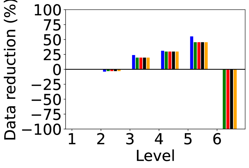
(a) LIPP

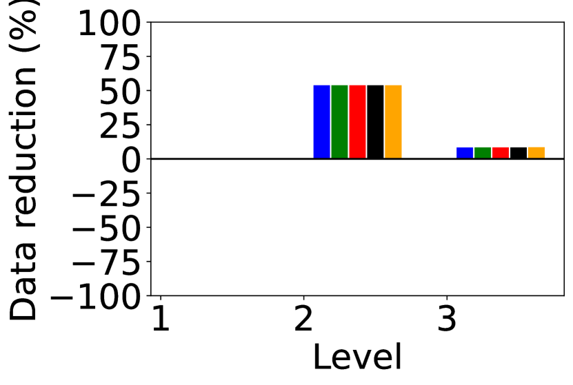
(b) ALEX

Figure 19: Data reduction percentage on Covid by level vs. insertion batches

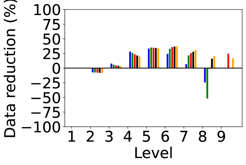
(a) LIPP

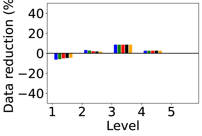
(b) ALEX

Figure 20: Data reduction percentage on OSM by level vs. insertion batches

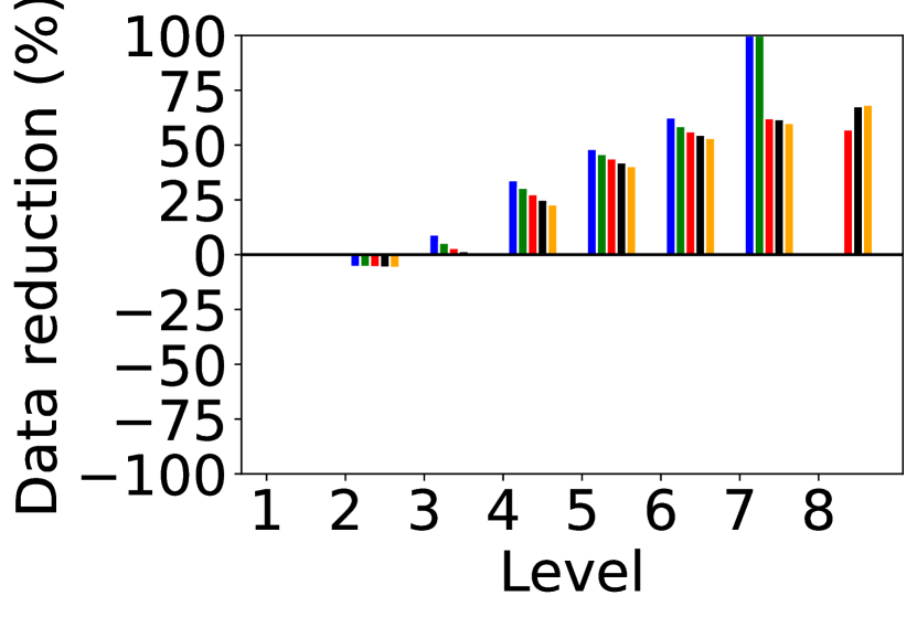
(a) LIPP

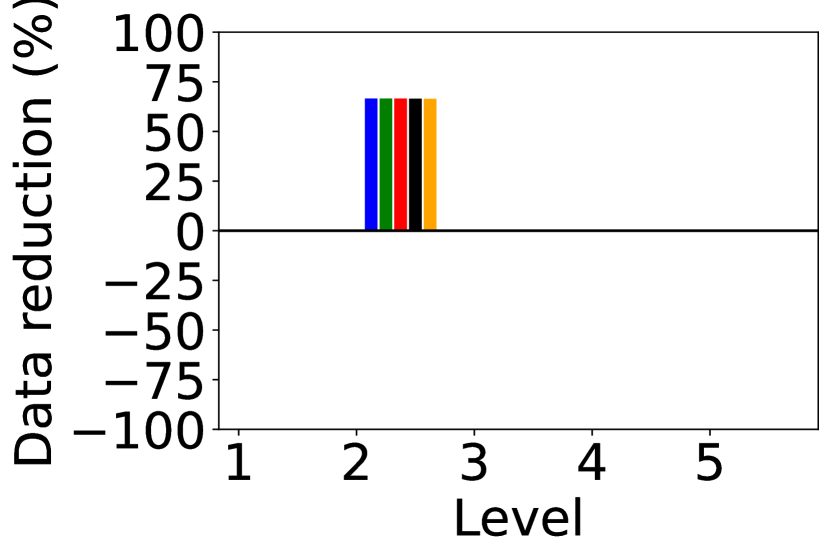
(b) ALEX

Figure 21: Data reduction percentage on Genome by level vs. insertion batches

VII Conclusion

We addressed the issue of indexing data of complex distributions by modifying the key set to be more favourable for index learning, instead of developing yet another indexing function or structure. To achieve this, we proposed a CDF smoothing technique via insertion of virtual points. Further, we proposed an algorithm named CSV to utilize this technique on existing hierarchical learned index structures, to improve the query time for keys in lower levels of these index structures. The proposed algorithm is implemented on three recent learned indexes, which are evaluated on real-world datasets. The results show significant query performance improvements, i.e., up to 34%, with a controllable and low storage space overhead.

References

- [1] T. Kraska, A. Beutel, E. H. Chi, J. Dean, and N. Polyzotis, “The case for learned index structures,” in SIGMOD, 2018, pp. 489–504.
- [2] J. Ding, U. F. Minhas, J. Yu, C. Wang, J. Do, Y. Li, H. Zhang, B. Chandramouli, J. Gehrke, D. Kossmann, D. Lomet, and T. Kraska, “ALEX: An updatable adaptive learned index,” in SIGMOD, 2020, p. 969–984.
- [3] P. Ferragina and G. Vinciguerra, “The PGM-index: A fully-dynamic compressed learned index with provable worst-case bounds,” Proceedings of the VLDB Endowment, vol. 13, no. 8, p. 1162–1175, 2020.
- [4] J. Wu, Y. Zhang, S. Chen, J. Wang, Y. Chen, and C. Xing, “Updatable learned index with precise positions,” Proceedings of the VLDB Endowment, vol. 14, no. 8, p. 1276–1288, 2021.
- [5] Z. Zhang, P.-Q. Jin, X.-L. Wang, Y.-Q. Lv, S.-H. Wan, and X.-K. Xie, “COLIN: A cache-conscious dynamic learned index with high read/write performance,” Journal of Computer Science and Technology, vol. 36, pp. 721–740, 2021.
- [6] V. Nathan, J. Ding, M. Alizadeh, and T. Kraska, “Learning multi-dimensional indexes,” in SIGMOD, 2020, p. 985–1000.
- [7] P. Li, H. Lu, Q. Zheng, L. Yang, and G. Pan, “LISA: A learned index structure for spatial data,” in SIGMOD, 2020, p. 2119–2133.
- [8] J. Ding, V. Nathan, M. Alizadeh, and T. Kraska, “Tsunami: A learned multi-dimensional index for correlated data and skewed workloads,” Proceedings of the VLDB Endowment, vol. 14, no. 2, p. 74–86, 2020.
- [9] Y. Ding, X. Zhao, and P. Jin, “An error-bounded space-efficient hybrid learned index with high lookup performance,” in DEXA, 2022, p. 216–228.
- [10] S. Pai, M. Mathioudakis, and Y. Wang, “WaZI: A learned and workload-aware Z-index,” in EDBT, 2024, pp. 559–571.
- [11] Y. Sheng, X. Cao, Y. Fang, K. Zhao, J. Qi, G. Cong, and W. Zhang, “WISK: A workload-aware learned index for spatial keyword queries,” Proceedings of the ACM on Management of Data, vol. 1, no. 2, pp. 187:1–187:27, 2023.
- [12] P. Li, Y. Hua, J. Jia, and P. Zuo, “FINEdex: A fine-grained learned index scheme for scalable and concurrent memory systems,” Proceedings of the VLDB Endowment, vol. 15, no. 2, p. 321–334, 2021.
- [13] C. Tang, Y. Wang, Z. Dong, G. Hu, Z. Wang, M. Wang, and H. Chen, “XIndex: A scalable learned index for multicore data storage,” in PPoPP, 2020, p. 308–320.
- [14] J. Ge, H. Zhang, B. Shi, Y. Luo, Y. Guo, Y. Chai, Y. Chen, and A. Pan, “SALI: A scalable adaptive learned index framework based on probability models,” Proceedings of the ACM on Management of Data, vol. 1, no. 4, pp. 258:1–258:25, 2023.
- [15] B. Lu, J. Ding, E. Lo, U. F. Minhas, and T. Wang, “APEX: a high-performance learned index on persistent memory,” Proceedings of the VLDB Endowment, vol. 15, no. 3, p. 597–610, 2021.
- [16] H. Lan, Z. Bao, J. S. Culpepper, R. Borovica-Gajic, and Y. Dong, “A simple yet high-performing on-disk learned index: Can we have our cake and eat it too?” arXiv preprint arXiv:2306.02604, 2023.
- [17] Z. Wang, C. Ding, F. Song, K. Lu, J. Wan, Z. Tan, C. Xie, and G. Li, “WIPE: A write-optimized learned index for persistent memory,” ACM Transactions on Architecture and Code Optimization,, vol. 21, no. 2, pp. 22:1–22:25, 2024.
- [18] A. Kipf, R. Marcus, A. van Renen, M. Stoian, A. Kemper, T. Kraska, and T. Neumann, “RadixSpline: a single-pass learned index,” in aiDM, 2020, pp. 5:1–5:5.
- [19] M. Mishra and R. Singhal, “RUSLI: Real-time updatable spline learned index,” in aiDM, 2021, p. 1–8.
- [20] A. Galakatos, M. Markovitch, C. Binnig, R. Fonseca, and T. Kraska, “FITing-Tree: A data-aware index structure,” in SIGMOD, 2019, p. 1189–1206.
- [21] Z. Sun, X. Zhou, and G. Li, “Learned index: A comprehensive experimental evaluation,” Proceedings of the VLDB Endowment, vol. 16, no. 8, p. 1992–2004, 2023.
- [22] C. Wongkham, B. Lu, C. Liu, Z. Zhong, E. Lo, and T. Wang, “Are updatable learned indexes ready?” Proceedings of the VLDB Endowment, vol. 15, no. 11, p. 3004–3017, 2022.
- [23] S. Wu, Y. Cui, J. Yu, X. Sun, T.-W. Kuo, and C. J. Xue, “NFL: Robust learned index via distribution transformation,” Proceedings of the VLDB Endowment, vol. 15, no. 10, p. 2188–2200, 2022.
- [24] J. Ge, B. Shi, Y. Chai, Y. Luo, Y. Guo, Y. He, and Y. Chai, “Cutting learned index into pieces: An in-depth inquiry into updatable learned indexes,” in ICDE, 2023, pp. 315–327.
- [25] J. Zhang and Y. Gao, “CARMI: A cache-aware learned index with a cost-based construction algorithm,” Proceedings of the VLDB Endowment, vol. 15, no. 11, p. 2679–2691, 2022.
- [26] L. Liu, C. Li, Z. Zhang, Y. Liu, K. Zhou, and J. Zhang, “A data-aware learned index scheme for efficient writes,” in ICPP, 2023, pp. 28:1–28:11.
- [27] M. Eppert, P. Fent, and T. Neumann, “A tailored regression for learned indexes: Logarithmic error regression,” in aiDM, 2021, p. 9–15.
- [28] Y. Li, D. Chen, B. Ding, K. Zeng, and J. Zhou, “A pluggable learned index method via sampling and gap insertion,” arXiv preprint arXiv:2101.00808, 2021.
- [29] E. M. Kornaropoulos, S. Ren, and R. Tamassia, “The price of tailoring the index to your data: Poisoning attacks on learned index structures,” in SIGMOD, 2022, p. 1331–1344.
- [30] M. Bachfischer, R. Borovica-Gajic, and B. I. Rubinstein, “Testing the robustness of learned index structures,” arXiv preprint arXiv:2207.11575, 2022.
- [31] R. Marcus, A. Kipf, A. van Renen, M. Stoian, S. Misra, A. Kemper, T. Neumann, and T. Kraska, “Benchmarking learned indexes,” Proceedings of the VLDB Endowment, vol. 14, no. 1, p. 1–13, 2020.
- [32] P. Van Sandt, Y. Chronis, and J. M. Patel, “Efficiently searching in-memory sorted arrays: Revenge of the interpolation search?” in SIGMOD, 2019, p. 36–53.
- [33] C. E. Lopez and C. Gallemore, “An augmented multilingual twitter dataset for studying the COVID-19 infodemic,” Social Network Analysis and Mining, vol. 11, no. 1, p. 102, 2021.
- [34] S2Geometry. (2024) The S2 Geometry library. [Online]. Available: http://s2geometry.io/
- [35] V. Pandey, A. Kipf, T. Neumann, and A. Kemper, “How good are modern spatial analytics systems?” Proceedings of the VLDB Endowment, vol. 11, no. 11, p. 1661–1673, 2018.
- [36] S. S. Rao, M. H. Huntley, N. C. Durand, E. K. Stamenova, I. D. Bochkov, J. T. Robinson, A. L. Sanborn, I. Machol, A. D. Omer, E. S. Lander et al., “A 3D map of the human genome at kilobase resolution reveals principles of chromatin looping,” Cell, vol. 159, no. 7, pp. 1665–1680, 2014.