High ground state overlap via quantum embedding methods

Abstract

Quantum computers can accurately compute ground state energies using phase estimation, but this requires a guiding state which has significant overlap with the true ground state. For large molecules and extended materials, it becomes difficult to find guiding states with good ground state overlap for growing molecule sizes. Additionally, the required number of qubits and quantum gates may become prohibitively large. One approach for dealing with these challenges is to use a quantum embedding method, which allows a reduction to one or multiple smaller quantum cores embedded in a larger quantum region. In such situations it is unclear how the embedding method affects the hardness of constructing good guiding states. In this work, we therefore investigate the preparation of guiding states in the context of quantum embedding methods. We extend previous work on quantum impurity problems, a framework in which we can rigorously analyze the embedding of a subset of orbitals. While there exist results for optimal active orbital space selection in terms of energy minimization, we rigorously demonstrate how the same principles can be used to define selected orbital spaces for state preparation in terms of the overlap with the ground state. Moreover, we perform numerical studies of molecular systems relevant to biochemistry, one field in which quantum embedding methods are required due to the large size of biomacromolecules such as proteins and nucleic acids. We investigate two different embedding strategies which can exhibit qualitatively different orbital entanglement. In all cases we demonstrate that the easy-to-obtain mean-field state will have a sufficiently high overlap with the target state to perform quantum phase estimation.

I Introduction

Some of the most promising applications for quantum computers arguably lie in their utility for molecular and materials science. These fields face important computational challenges, in both academic and industrial settings. Prominent examples can be found in catalysis, battery and drug design [1, 2, 3, 4], and biochemistry [5, 6]. True quantum advantage will likely only emerge in the fault-tolerant regime, where quantum phase estimation (QPE) algorithms will allow for energy calculations of a quantum system (i.e., a molecule or material) with controlled and guaranteed accuracy.

One of the central problems of quantum chemistry is the computation of ground-state electronic energies. We consider a system with a fixed number $n$ of electrons, and a discretization of the electronic structure problem in the Born-Oppenheimer approximation into $N$ spin-orbitals, giving a Hamiltonian of the form

$$H=\sum_{pq=1}^{N}h_{pq}a_{p}^{{\dagger}}a_{q}+\frac{1}{2}\sum_{pqrs=1}^{N}g_{pqrs}a_{p}^{{\dagger}}a_{r}^{{\dagger}}a_{s}a_{q}\,,$$

where $a_{p}$ for $p=1,\dots,N$ are the fermionic annihilation operators for the $N$ spin-orbitals and $g_{pqrs}=(pq|rs)$ are the two-body integrals, see for example [7] for details. A system with $N$ spin-orbitals and $n$ electrons has a Hilbert space of dimension ${N\choose n}$ which is exponential in $N$ if $n$ scales linearly with $N$. High accuracy classical methods struggle with the size of this Hilbert space. The key advantage of quantum computing is that the quantum computer can natively represent states in the Hilbert space using only $N$ qubits. When considering the scaling with system size, one should keep in mind that at fixed electron number $n$, but an increasing number of orbitals $N$ (the continuum limit), the Hilbert space dimension increases only as $\operatorname{poly}(N)$ (polynomially in $N$), albeit with an in practice prohibitive exponent $n$.

There are two major challenges in quantum computing for chemistry and many-body physics.

1. The first challenge is the orthogonality catastrophe. Quantum phase estimation requires an initial guiding state which has sufficient overlap with the ground state. However, for systems with large $N$ and scaling electron number, small local errors in the guiding state lead to an exponential decay in the overlap with the global ground state. As a result good guiding states become hard to find, see Appendix A.

2. The second challenge is to perform Hamiltonian simulation for a time $\mathcal{O}(\varepsilon^{-1})$ to achieve quantum phase estimation precision $\varepsilon$, and to reduce the dependence of the computational cost on $N$.

The first challenge is a fundamental and theoretical obstruction to computing ground state energies efficiently on a quantum computer. However, for many molecules, conventional computational methods are observed to find good guiding states in practice (though this may be different for strongly correlated materials with a lattice structure), so for practical applications to quantum chemistry there is evidence that this is not the main problem [8, 9] and our work supports this claim. For the second challenge, the scaling of the Hamiltonian simulation subroutine in the phase estimation algorithm is polynomial in $N$, and can in theory be performed efficiently on a quantum computer. However, this scaling can lead to quantum circuits with a prohibitively large gate count in practice and represents a serious bottleneck for useful quantum computations. Concretely, from state-of-the-art resource estimates [2, 10, 3] it seems that with fault-tolerant devices, computations for 100 - 200 spin orbitals already require very extensive quantum resources (although it is difficult to precisely predict specifications of future fault-tolerant quantum computers).

Given a choice of orbital basis, the electronic ground state can be written as

$$\ket{\Psi}=\sum_{i}C_{i}\ket{\Phi_{i}},\quad\sum_{i}\absolutevalue{C_{i}}^{2}=1$$ (1)

where the sum runs over Slater determinants $\ket{\Phi_{i}}$. For example, one can choose Hartree-Fock (HF) orbitals. In that case, the expansion in Eq. 1 consists of the HF state $\ket{\Phi_{0}}$ and corrections to it, which represent electron correlations. One can also choose a different orbital basis, and this may lead to a significant increase in the largest weight on a single determinant. If the HF basis state qualitatively misrepresents the ground state, and there are more determinants with weights of the same order of magnitude, this is known as static correlation. The remaining determinants with small weights then account for the so-called dynamical correlation. While useful notions, there is no sharp distinction between dynamical and static correlation.

The question of finding and preparing good guiding states is closely related to the computational complexity of the electronic structure problem. The problem of finding ground state energies of local Hamiltonians in full generality is QMA-hard [11, 12], so this task is believed to be intractable even for quantum computers. In particular, this implies that it is hard to prepare guiding states with non-trivial ground state overlap — however, numerical evidence suggests that finding good guiding states is feasible for many realistic not-too-large chemical systems [8, 13]. This is the case if the correlation is of a dynamical nature, and also in systems with a static correlation; a small number of determinants [9], choosing a different orbital basis (see, for instance, Ref. [14]), or symmetry-respecting configuration state functions [15] may suffice to reach good ground state overlap and hence yield efficient quantum phase estimation algorithms. For quantum phase estimation, a constant (or even inverse polynomially small) ground state overlap suffices for efficient ground state energy computation. For the total cost, it does not make a significant difference whether one has a constant ground state overlap, or even ground state overlap close to 1. However, if the guiding state has ground state overlap close to 1, this allows the possibility to paralellize the phase estimation into multiple circuits of shorter depth [16, 17], as we briefly review in Appendix A, and which may be particularly useful for early fault-tolerant quantum computers.

In many large molecules where static quantum correlations are important, so that a mean-field treatment does not suffice to represent the target state even qualitatively well, these correlations can be assigned to a relatively small number of orbitals. If these orbitals are localized in three-dimensional space, static correlation will be of a short-ranged nature. In such situations, both challenges (ground state overlap and Hamiltonian simulation scaling with $N$) can be addressed by using an appropriate embedding method, which singles out a spatial region (or length scale) that is treated fully quantum mechanically, and an environment (or longer range correlations) which can be treated with an approximate electronic structure model such as (mean-field) Hartree-Fock (HF) or some other electronic structure model of low computational complexity such as (variants of) Kohn-Sham density functional theory (DFT). By focusing on a smaller embedded quantum subsystem (denoted as a quantum core in the following), the system to which one applies phase estimation is sufficiently small so that the exponential scaling of the orthogonality catastrophe has not yet kicked in, and one can still find high-overlap guiding states using classical methods. Additionally, the smaller number of orbitals leads to a reduced gate count in the phase estimation quantum circuit. For very large molecules (such as proteins, protein complexes, or interacting biomolecules in biochemistry), embedding strategies can be of a multi-level nature, where the description of the interatomic interactions ranges from classical force fields to different quantum mechanical approximations. We provide a brief introduction to relevant aspects of quantum embedding theory in Section II.

In this work we focus on quantum-in-quantum embedding schemes, where a large system is described by an approximate quantum mechanical model (such as HF or Kohn-Sham DFT), while one or more subsystems embedded into this large system define the quantum cores. The energy contribution of the quantum cores to the full potential energy surface of the large system can be rigorously obtained by a (future) fault-tolerant quantum computer using a representation of the full wavefunction in the restricted orbital space of the quantum cores. It is for this reason that we consider state preparation in the context of quantum embedding approaches.

While wave function-based approaches in traditional computing (such as coupled cluster theory or multi-configurational approaches with multi-reference perturbation theory) can deliver accurate quantum core energies, an important drawback is that precise and controllable error bounds are not known for any of these methods [18]. By contrast, quantum computation based on phase estimation can deliver total electronic energies to a given precision (that is, typically chemical accuracy between 1 and 0.1 mHartree) — provided that an initial guiding state can be efficiently prepared which will have a large overlap with the target state that is to be determined. We emphasize that rigorous error estimates will be a key advantage over traditional approaches [1, 19, 20], apart from the fact that a quantum computer with a sufficiently large number of qubits for the representation of an electronic state will tame the curse of dimensionality posed to traditional approaches.

The use of embedding methods for quantum computing in quantum chemistry raises important questions:

1. What is the interplay between an embedding method and the guiding state? For example, if the choice of the embedding method affects the type of correlation on the resulting orbital space in a quantum core, then this may have consequences for the character of the guiding state up to the point where it might be difficult to determine.

2. What is the computational complexity of problems with localized quantum correlations?

The second question concerns the general computational complexity of problems with localized quantum correlations. In Section III, we study this question theoretically in the context of quantum impurity models, specifically by extending the work of [21] on the nature of quantum impurity problems to shed light on these questions. A quantum impurity model is a system with a scaling number of $N$ orbitals, of which only a constant number $M$ participate in two-body interactions. Such models may be considered a useful description for systems where electron correlation is localized to a small subset of orbitals. Based on [21], we show that there exist good quantum embeddings for such systems. Based on this, we propose an approach to the guiding state problem where one uses an embedding method to find a guiding state which is an arbitrary state on the quantum core, and a Slater determinant on the environment. We show that if one chooses a good embedding or if the one-body Hamiltonian is gapped, this guiding state has at least an inverse polynomial overlap with the true ground state of the embedding Hamiltonian, giving a polynomial quantum algorithm for the ground state energy. This is in contrast to the best-known rigorous classical algorithms, which in these cases have a quasi-polynomial scaling in the precision [21].

These results motivate a general strategy for preparing guiding states for problems with localized quantum correlations on large-scale fault-tolerant quantum computers. We propose that one searches for guiding states through quantum-in-quantum embeddings. Here, one identifies an active orbital space $A$ and an environment $C$, and takes as a guiding state a state of the form $\ket{\Phi_{A}}\wedge\ket{\Psi_{C}}$, where $\ket{\Phi_{A}}$ is the solution to the (small) active space problem, and $\ket{\Psi_{C}}$ is a Slater determinant on the environment. Quantum phase estimation then allows for accurate computation of the ground state energy.

We demonstrate numerically in Section IV that for two conceptually different embedding methods, one can find low-complexity guiding states, even though the two different methods produce rather different orbital bases. For this demonstration we focus on small biomolecules (tryptophan and its oligopeptide structures), which occur as monomers and oligomers in biomacromolecules (proteins), and on a transition-metal drug that can form a host-guest complex with a protein. Such complexes are key to molecular recognition processes. While we focus on biomolecules, our approach is similarly relevant in other application areas involving larger molecules or materials.

II Quantum embedding methods

In order to make computations feasible for large systems, for which physical or chemical properties are governed by a relatively small spatial regions within the larger system, an established approach (see, for instance [22, 23]) is to treat different subsystems or length scales at different levels of accuracy. For example, in the case of molecular recognition, it may be sufficient to focus on the interaction seam of host and guest molecules and, hence, to take into account electron correlation accurately only in the binding region. Embedding theory deals with approaches to embed approximations of different levels of accuracy into one another; see [24, 25, 26, 27, 28, 29] for reviews of quantum embedding theory. In general, one decomposes the system into a quantum core, where one uses a high-level electronic structure model, which takes into account the more complex nature of the wavefunction, and a (quantum or classical) environment. If feasible, the environment can be treated using a low-level model such as HF or DFT. It is possible to have multiple quantum cores and multiple embedding layers, treating parts of the system at the level of classical force fields, semi-empirical methods, or DFT at different levels of accuracy. In order to take the effect of the environment into account, an embedding scheme requires the construction of an effective Hamiltonian on the quantum cores, given the solution of the low-level solver. Given the result of minimizing this Hamiltonian on the quantum cores, the embedding scheme should provide a prescription for a global energy estimate.

We will discuss two different embedding schemes, which we compare in detail with molecular examples in Section IV. The first approach is based on density matrices. This is natural for quantum computing, since quantum computation naturally interfaces with quantum states. For example, the bootstrap embedding (a particular density matrix-based embedding scheme), one can enforce the consistency conditions between overlapping fragments on the quantum computer [30]. As an alternative, we also consider projection-based embedding methods. These have the advantage of being naturally compatible with DFT, which may be useful for multiscale approaches.

II.1 Embedding based on density matrices

A natural approach toward embedding emerges from the framework of open-system quantum theory and is based on density matrices; an example is density matrix embedding theory (DMET) [31, 32, 33, 34], see [35] for a precise mathematical description. Here we consider a system with $N$ orbitals, where we identify subsets $A_{1},\dots,A_{n}$ of these orbitals, which may be called ‘fragments’ or ‘impurities’. We let $M_{i}$ be the number of orbitals in $A_{i}$. Depending on the method, these fragments may overlap or not. Whereas the formal basis of DMET is the Schmidt decomposition, its key practical idea is to combine a high-level solver on the fragments with a mean-field solution on the global level and enforce consistency conditions. We start with a global state given by a single Slater determinant $\ket{\Psi}$, which can be obtained as the Hartree-Fock solution by the low-level solver. For each of the subsystems $A_{i}$ we can perform a Schmidt decomposition, which for each $i$ gives a decomposition of the the full $N$-dimensional single-particle space into $A_{i}$ (the fragment orbitals), a ‘bath’ $B_{i}$ for $A_{i}$ of size at most $M_{i}$ (the bath orbitals) and its complement $C_{i}$, such that the state

$$\ket{\Psi}=\ket{\Psi_{A_{i}B_{i}}}\wedge\ket{\Psi_{C_{i}}}$$

is decomposed into Slater determinants $\ket{\Psi_{A_{i}B_{i}}}$ and $\ket{\Psi_{C_{i}}}$ on $A_{i}B_{i}$ and $C_{i}$ respectively. Now, one may look for wavefunctions of the form $\ket{\Psi_{i}}=\ket{\Phi_{A_{i}B_{i}}}\wedge\ket{\Psi_{C_{i}}}$ where $\ket{\Phi_{A_{i}B_{i}}}$ is now an arbitrary fermionic state on $A_{i}B_{i}$, determined by a high-precision solver (such as a quantum computer). The high-level solver minimizes the energy over states of this form. Since we have a fixed Slater determinant $\ket{\Psi_{C_{i}}}$ on $C_{i}$, this gives an effective Hamiltonian on $A_{i}B_{i}$

$$H_{A_{i}B_{i}}=\left(I\otimes\bra{\Psi_{C_{i}}}\right)H\left(I\otimes\ket{\Psi_{C_{i}}}\right).$$

This Hamiltonian is such that

$$\min_{\ket{\Psi_{i}}}\bra{\Psi_{i}}H\ket{\Psi_{i}} =\min_{\ket{\Phi_{A_{i}B_{i}}}}\bra{\Phi_{A_{i}B_{i}}}H_{A_{i}B_{i}}\ket{\Phi_{A_{i}B_{i}}}$$

where the minimization on the left-hand side is over states of the form

$$\ket{\Psi_{i}}=\ket{\Phi_{A_{i}B_{i}}}\wedge\ket{\Psi_{C_{i}}}.$$

There are different schemes for estimating a global energy based on density matrix embedding. The standard approach is to try to achieve self-consistency between the global Slater determinant and the fragment wavefunctions. Here, one takes non-overlapping fragments and searches for a solution where the Slater determinant $\ket{\Psi}$ has the same 1-RDMs on the fragments $A_{i}$ as the fragment solutions $\ket{\Phi_{A_{i}B_{i}}}$. This can be obtained by iteratively solving for the fragments and updating them to a global mean-field solution with constrained 1-RDMs. A different approach is the bootstrap embedding, where one takes overlapping fragments and iteratively tries to enforce consistency between the fragments on their overlap instead of with a global state, see [36, 37, 38] for details. However, we note that in both cases, there is no guarantee of the existence of a global wavefunction compatible with these schemes, and the results are not variational. This means that the obtained value is not necessarily a strict upper bound on the true ground state energy.

II.2 Embedding based on projection

An alternative approach is given by projection-based embeddings [39, 40]. Here, we use a method based on the Huzinaga equation [41, 39]. We describe the case with a single quantum core. We start the theory discussion with HF as the low-level solver, highlighting the similarities to DMET. Later will we describe how DFT retrieves the missing electron correlation in Hartree-Fock, making the approach formally exact. The exactness of the approach means that when using the exact (unknown) exchange correlation functional for the DFT computation, and the exact wave function solution on the embedded fragment, the result of following the embedding procedure equals the exact ground state energy. This embedding method starts from a HF (or from a Kohn-Sham density functional theory calculation), yielding a collection of molecular orbitals indexed by a set $J$ and a single Slater determinant $\ket{\Phi}$ with the orbitals in $\mathcal{N}\subseteq J$ occupied. Given these orbitals $\phi_{j}$, they are partitioned into two sets $A$ and $C$ of active and environment orbitals. We write $\mathcal{N}_{A}$ and $\mathcal{N}_{C}$ for the subsets of occupied orbitals in $\ket{\Phi}$. The division into $A$ and $C$ is often based on the localization of the orbitals on specific atoms in the molecule [40, 39]. Alternatively, a unitary transformation in $\mathcal{N}$ may be transformed to enforce a localization on specific atoms [42], or an automated orbital analysis can be performed to identify orbitals contributing strongly to energy differences [43]. The idea of the projection-based embedding is now again to try to solve the minimization problem

$$\min_{\ket{\Psi}}\bra{\Psi}H\ket{\Psi}\qquad\ket{\Psi}=\ket{\Phi_{A}}\wedge\ket{\Psi_{C}}$$

where $\ket{\Phi_{A}}$ is an arbitrary state on $A$ and $\ket{\Psi_{C}}$ is the Slater determinant on the environment where the orbitals in $\mathcal{N}_{C}$ are occupied. Similarly to the embedding based on density matrices, the Slater determinant on the environment is kept fixed, which yields the effective Hamiltonian for the fragment

$$H_{A} =\left(I\otimes\bra{\Psi_{C}}\right)H\left(I\otimes\ket{\Psi_{C}}\right)$$

$$=\bar{E}+\sum_{p,q\in A}h^{(A\text{in}C)}_{pq}a^{\dagger}_{p}a_{q}+\frac{1}{2}\sum_{\begin{subarray}{c}p,q\\ r,s\in A\end{subarray}}(pq|rs)a^{\dagger}_{p}a^{\dagger}_{r}a_{s}a_{q},$$

where

$$\bar{E}=2\sum_{p\in\mathcal{N}_{C}}h_{pp}+\sum_{p,q\in\mathcal{N}_{C}}[2(pp|qq)-(pq|qp)]$$

is the mean-field energy of the environment, and

$$h^{(A\text{in}C)}_{pq}=h_{pq}+\sum_{c\in\mathcal{N}_{C}}[2(pq|cc)-(pc|qc)]$$

is the effective one-electron operator that includes the interaction between the fragment and the environment. In this case, both the environment energy and the fragment-environment interactions are captured on a mean-field level only, neglecting the correlation, while the overall energy is represented as $E=\bar{E}+E^{A\text{in}C}$, where $E^{A\text{in}C}$ is the energy of $h^{(A\text{in}C)}$. Note that the Hamiltonian $H_{A}$ on the quantum core has as two-body terms precisely the two-body terms acting on $A$, and only the one-body term is modified.

The key idea of the projection-based embedding is to recover the missing correlation using DFT. For this purpose, densities $\gamma$ from the initial DFT calculation are used to define the interaction terms between the fragment and the environment as

$$v_{\text{emb}}[\gamma^{A},\gamma^{C}] =g[\gamma^{A}+\gamma^{C}]-g[\gamma^{A}]$$

where $g$ is defined by

$$(g[\gamma])_{pq}=\sum_{ij}\gamma_{ij}\left[(pq|ij)-\frac{1}{2}x(pi|qj)\right]+\left(v_{\text{xc}}[\gamma]\right)_{pq}.$$

Here, $x$ is the fraction of the exact exchange in the exchange-correlation functional and $v_{\text{xc}}$ is the exchange-correlation potential matrix. This interaction term is used to redefine the effective one-electron operator as

$$\tilde{h}^{(A\text{in}C)}_{pq}= h_{pq}+\left(v_{\text{emb}}[\gamma^{A},\gamma^{C}]\right)_{pq}$$

$$-\left((F^{A}-\mu)P^{C}-P^{C}(F^{A}-\mu)\right)_{pq},$$

where $P^{C}$ is the matrix of the projection operator onto the subspace $C$, $\mu$ is a positive constant energy shift and $F^{A}$ is the Fock matrix for the embedded fragment. The last two terms are used to ensure that there is no mixing of the fragment and the environment orbitals. The overall energy of the system can be written as

$$E= \bra{\Psi_{A}}\tilde{H}_{A}\ket{\Psi_{A}}-\bra{\Psi_{A}}\hat{v}_{\text{xc}}[\gamma^{A}+\gamma^{C}]-\hat{v}_{\text{xc}}[\gamma^{C}]\ket{\Psi_{A}}$$

$$+E_{\text{xc}}^{\text{DFT}}[\gamma^{A}+\gamma^{C}]-E_{\text{xc}}^{\text{DFT}}[\gamma^{A}]-E_{\text{xc}}^{\text{DFT}}[\gamma^{C}]$$

$$+E^{\text{DFT}}[\gamma^{C}],$$

where $E^{\text{DFT}}[\gamma^{C}]$ is the Kohn-Sham DFT energy of $C$, $E_{\text{xc}}^{\text{DFT}}[\gamma]$ is the exchange-correlation functional evaluated for the density $\gamma$, and $\hat{v}_{\text{xc}}[\gamma]$ is the operator belonging to $v_{\text{xc}}$. Note that $E_{\text{xc}}^{\text{DFT}}[\gamma]$ is typically nonlinear in $\gamma$, which means that it cannot be calculated as the expectation value of $\hat{v}_{\text{xc}}[\gamma]$. Therefore, we formally subtracted the term $\bra{\Psi_{A}}\hat{v}_{\text{xc}}[\gamma^{A}+\gamma^{C}]-\hat{v}_{\text{xc}}[\gamma^{C}]\ket{\Psi_{A}}$ and added the differences in $E_{\text{xc}}^{\text{DFT}}[\gamma]$.

II.3 Embedding methods and quantum computing

Using appropriate embedding methods will be crucial for the application of quantum computers to chemical systems, especially for biochemistry, nanochemistry, and materials science. Identifying the right quantum mechanical subsystem of a molecule and using the quantum chemistry calculation on this fragment to derive conclusions about the full system is unavoidable for practical applications of quantum computation. The quantum computer then serves as the high-level solver in the embedding scheme.

Previous work using density matrix-based embedding schemes includes [44, 45, 46, 30, 47], approaches using projection-based embeddings include [48, 49, 50], and approaches based on Green’s functions are presented in Refs. [51, 52] (which we do not discuss in this work). These previous works have mostly focused on reducing the problem size, and running heuristic variational algorithms on (near-term) quantum computers. How the embedding method influences the problem of finding good guiding states, and thereby the prospects for phase estimation, has not been explored systematically in previous work to the best of our knowledge; one work in this direction is [5] which computes guiding state overlaps for a range of active space sizes for phase estimation for a protein system.

III Orbital selection for state preparation in quantum impurity problems

In this section, we aim at deriving rigorous results for the state preparation problem in an embedding situation. In order to accomplish this, we exploit the framework of quantum impurity problems. A quantum impurity model is a fermionic Hamiltonian which has arbitrary one-body interactions, and two-body interactions on a constant-sized subset of orbitals. Quantum impurity models are relevant as models in material science where there is an impurity in the material. A famous example is the Anderson impurity model [53] which describes a magnetic impurity in a metal. This model gives an explanation for the Kondo effect and has been instrumental in the development of numerical renormalization group techniques [54]. Besides the important application to impurities in metals, one can also consider them as a toy model for large molecules where mean-field approximations are accurate outside of a small interaction region. For example, the ‘impurity’ may consist of the orbitals which are localized in the binding region. Note that in the quantum impurity model, we assume that away from the impurity we have a one-body Hamiltonian (which is a different assumption than having an accurate mean-field approximation).

More formally, a quantum impurity model is defined by a fermionic Hamiltonian of the form $H_{\operatorname{free}}+H_{\operatorname{imp}}$ where $H_{\operatorname{free}}$ is a one-body Hamiltonian on $N$ fermionic modes, whereas $H_{\operatorname{imp}}$ is an interacting fermionic Hamiltonian acting on a subset of $M$ modes

$$H_{\operatorname{free}} =\sum_{pq=1}^{N}h_{pq}a_{p}^{\dagger}a_{q}$$

$$H_{\operatorname{imp}} =\sum_{pqrs=1}^{M}h_{pqrs}a_{p}^{\dagger}a_{q}^{\dagger}a_{r}a_{s}$$

Typically we consider constant $M$ and a scaling total system size $N$. We assume that $H_{\operatorname{free}}$ has single-particle energies in a constant range (which we can always achieve by rescaling). We write $\omega$ for the ground state energy gap of $H_{\operatorname{free}}$. If the Hamiltonian is number-conserving, we can study the lowest-energy state in the subspace where we fixed the number of particles to $n$.

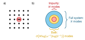
Figure 1: (a) A lattice model for the electrons in a metal, with an impurity at one site. (b) Illustration of Theorem III.1: the ground state can be accurately approximated by a state which is a Slater determinant on the environment and some unconstrained state on the fragment and bath modes.

Quantum impurity models are a simple but nontrivial class of models which capture the orthogonality catastrophe and the quality of embedding methods. The Anderson derivation of the orthogonality catastrophe [55], see Appendix A, suggests that the scaling of the orthogonality catastrophe may be polynomial rather than exponential for quantum impurity problems. For quantum phase estimation an inverse polynomial overlap suffices to get a polynomial algorithm, so this suggests that quantum impurity problems may be in BQP.

Secondly, from the perspective of embedding methods, since the impurity is small compared to the system size, one may hope that one can identify a bath of a relatively small number of orbitals which are influenced by the impurity, and one can solve the full system by restricting to this bath.

Quantum impurity problems have been studied rigorously by Bravyi and Gosset in [21]. Their main technical result is a bound on the decay of the eigenvalues of the 1-RDM. This gives rise to approximations of the ground state by a relatively small number of Gaussian states. As an application, [21] gives a quasipolynomial classical algorithm for the ground state energy, and shows that the quantum impurity problem is in QCMA, which is the class of problems which can be efficiently verified by a quantum computer given a classical witness, and which is between NP and QMA.

Our results build on this work in two ways. Firstly, we argue that under certain conditions one can find an efficiently preparable state which has inverse polynomial overlap with the ground state, giving an efficient quantum algorithm for the ground state energy.

Secondly, the results in [21] are formulated in terms of Gaussian states rather than Slater determinants. In order to relate their results to usual approaches to embedding methods in quantum chemistry, we derive the analagous statements using Slater determinants, working at a fixed particle number. A detailed description of the set-up, as well as formal statements and proofs are provided in Appendix C.

III.1 Decay properties of the one-body reduced density matrix and good embeddings

One-electron basis states (orbitals) are key to understanding different embedding techniques [56]. Given an electronic structure Hamiltonian on a set of orbitals and a fixed number of electrons, orbitals are often partitioned into sets that are called frozen (doubly occupied), active, and virtual (unoccupied). The idea is that, in an expansion of the wavefunction as in Eq. 1, only the frozen and a few additional orbitals (that is, the active ones) give rise to determinants with large weights $\alpha_{i}$. This means that the problem reduces to an effective problem defined only on the active space. The frozen and virtual spaces may contribute to the dynamical correlation, but this can be accounted for by a computationally less intensive method method (for example, by perturbation theory). The selection of the active orbitals can be based on various measures such as natural orbital occupation numbers [57, 58, 59, 60] or information entropy based [61, 62, 63, 64]. Our formal analysis will focus on the former in the following, whereas for practical reasons, our numerical results will exploit the latter, which can be based on localized orbitals that can have advantages over natural orbitals. In any case, as we show in the appendix, orbital rotations are always possible, which would allow one to exploit natural orbitals for state preparation, which can then be rotated into a local basis.

Given a ground state $\ket{\Psi}$, the one-body reduced density matrix (1-RDM), or covariance matrix, is the matrix $\gamma$ defined by $\gamma_{pq}=\bra{\Psi}a_{p}^{\dagger}a_{q}\ket{\Psi}$. Its eigenvectors define a set of orbitals known as the natural orbitals. We order the eigenvalues of $\gamma$ as $1\geq\sigma_{1}\geq\sigma_{2}\geq\dots\geq\sigma_{N}\geq 0$. The eigenvalue $\sigma_{j}$ equals the expected particle number for natural orbital $j$. This means that the natural orbitals for which $\sigma_{j}$ equals zero or one are always unoccupied or occupied respectively in the ground state. If the eigenvalue $\sigma_{j}$ is close to zero or one, we may approximate the ground state by a state where the corresponding natural orbital is unoccupied or occupied respectively. In other words, if we can bound the number of orbitals for which $\sigma_{j}$ is not close to zero or one by $K$, then we can approximate the ground state $\ket{\Psi}$ by a state $\ket{\tilde{\Psi}}=\ket{\Phi}\wedge\ket{\Theta}$ where $\ket{\Theta}$ is a Slater determinant and $\ket{\Phi}$ is an arbitrary state on $K$ modes. This means that these $K$ modes define a good active space for the problem at hand, and we can reduce the problem of (approximately) computing the ground state energy to this subspace.

The main result of [21] is a bound on the eigenvalues of the 1-RDM of quantum impurity problems, which is used to approximate the ground state in terms of Gaussian states. For chemistry problems we typically have a fixed number of electrons, and it is more convenient to work with Slater determinants. We adapt the argument of [21] to show the following result, which we prove in Appendix C.

Theorem III.1.

Let $\omega>0$ be the ground state energy gap of $H_{\operatorname{free}}$, and let $\varepsilon>0$. Then for

$$K=\mathcal{O}\left(\log(\omega^{-1})\left(\log(\varepsilon^{-1})+\log\log(\omega^{-1})\right)\right)$$

there exists a Slater determinant $\ket{\Theta}$ on $N-K$ modes and an arbitrary state $\ket{\Phi}$ on $K$ modes such that the state

$$\ket{\tilde{\Psi}}=\ket{\Phi}\wedge\ket{\Theta}$$

has overlap $\absolutevalue{\braket{\tilde{\Psi}}{\Psi}}\geq 1-\varepsilon$ with a ground state $\ket{\Psi}$ of $H_{\operatorname{free}}+H_{\operatorname{imp}}$.

Note that while this result shows that there exists a good active space, it only provides a good way to determine which orbitals make up this active space given the ground state 1-RDM (which one does not necessarily have access to without a priori knowledge of the ground state). In practice, finding good active spaces is based on using an efficient classical method to approximate the 1-RDM and using this estimate to select an appropriate accurate space as discussed in Section II.

III.2 Computational complexity of the quantum impurity problem

The general electronic structure problem is QMA-complete [65, 12], meaning that it is likely a hard problem even for quantum computers. On the other hand, Hamiltonians with only one-body interactions, like $H_{\operatorname{free}}$, can be efficiently simulated classically [66]. An important broad question in quantum computing is to determine the existence of (physically relevant) families of Hamiltonians for which the ground state problem is in BQP, while computing the ground state energy is hard classically. Proving such a separation is difficult (as this would imply a separation between P and BQP), but one can at least try to prove BQP containment for specific families of Hamiltonian ground state energy problems for which we do not know rigorous polynomial-time classical algorithms, see for example [67, 68].

We investigate the quantum computational complexity of quantum impurity problems. Here, the goal is to approximate the ground state energy of an impurity problem on $N$ modes, with a constant-sized impurity, to precision $\varepsilon$. As we saw in the previous section, for quantum impurity problems there exist relatively small active spaces, significantly reducing the size of the problem. It was shown in [21] that this can be leveraged to give a classical algorithm which scales polynomially in $N$ and quasipolynomially in the precision $\varepsilon$, with overall scaling $\mathcal{O}(N^{3})\exp(\mathcal{O}(\log(\varepsilon^{-1})^{3}))$. It is also shown that the ground state energy problem for quantum impurity models is contained in QCMA, the class of problems for which a quantum computer can efficiently verify solutions given a classical witness. QCMA-hard problems are unlikely to be solvable efficiently on a quantum computer. This leaves the interesting open problem whether one can prove whether quantum computers can efficiently approximate the ground state energy of quantum impurity problems to polynomial precision. We argue that under two different restrictions, quantum impurity problems become easy for quantum computers (while not obviously so for classical algorithms).

The main observation is that when we apply Theorem III.1, it suffices to find an active space such that the ground state overlap is constant (but not close to 1). If this active space contains only a constant number of orbitals $K$, then we may consider the state $\rho$ corresponding to choosing a random active space of size $K$ and preparing the maximally mixed state for this active space. For constant $K$, this leads to a ground state overlap which is at least $\operatorname{poly}(N)^{-1}$, and hence $\rho$ can be used as a guiding state to yield a polynomial time algorithm. Indeed, Theorem III.1 gives a constant-sized active space for constant precision if the gap $\omega$ is constant. As a further comment, these assumptions change the scaling of the classical algorithm of [21] to $\mathcal{O}(N^{3})\exp(\mathcal{O}(\log(\varepsilon^{-1})^{2}))$ in the case of constant gap. This provides evidence that quantum impurity models may provide an example class of systems with polynomial time quantum algorithm, but no polynomial time classical algorithm. However, the precise status of this remains unclear, in particular since there is already a classical algorithm with quasipolynomial scaling, and an improved analysis or better classical algorithm could lead to polynomial scaling. Moreover, the potential advantage disappears if the full quantum impurity Hamiltonian is gapped, as [21] provides a polynomial classical algorithm for that situation based on matrix product states (MPS).

A second simplification arises in the case where we have a sufficiently accurate approximation of the 1-RDM of a ground state. In this case, we can construct an active space on $\log(\omega^{-1})$ orbitals which suffices for a constant overlap with the ground state. Since this active space has polynomial dimension, the maximally mixed state on this subspace gives a sufficiently good guiding state for phase estimation. We summarize these findings with the following result, formally stated an proven as Theorem C.3 in Appendix C.

Theorem III.2.

The quantum impurity problem for $H=H_{\operatorname{free}}+H_{\operatorname{imp}}$ is in BQP if either $H_{\operatorname{free}}$ has a constant gap, or if the ground state 1-RDM is given.

Of course, one generally needs the ground state in order to compute the 1-RDM, so if one requires it beforehand then this does not directly lead to a useful algorithm. The above result should however be seen as evidence for the usefulness of iterative approaches, where one starts with some estimate of the 1-RDM using computationally inexpensive classical means, and then uses a quantum computer to perform a calculation which leads to a more accurate approximation of the 1-RDM. See [52] for a practical proposal for such a scheme.

The algorithms in Theorem III.2 and their analysis do not directly lead to practically useful approaches, as their polynomial scaling can be of high degree. However, these results should be seen as a proof of principle that in quantum impurity problems the ‘orthogonality catastrophe’ is of a relatively mild nature and may not be an insurmountable problem, reducing a potentially exponential scaling to a polynomial one. In practice, one can likely find better guiding states than the maximally mixed states in the above theoretical algorithms. Of course, classical algorithms for impurity problems will also perform much better than currently proven by rigorous guarantees [69, 70, 71].

Given a large system of $N$ orbitals, where we know that the problem has a strong electron correlation in some subsystem, one can use a quantum embedding method (such as described in Section II) to find a reasonable active space $A$ of $K$ modes, and an environment system $C$. One then uses a classical method to find a good guiding state $\ket{\Psi_{A}}$ on this small active space, and a Slater determinant $\ket{\Psi_{C}}$ on $C$, and uses $\ket{\Psi_{A}}\wedge\ket{\Psi_{C}}$ as guiding state on the full system. Theorem III.1 shows that for a quantum impurity model there exist good guiding states of this form, but it does not guarantee that one finds the right subsystem $A$ or state $\ket{\Psi_{A}}$ in this way.

Finally, we note that the concept of impurity models has also been used to compute properties of strongly correlated materials, as in the Hubbard model. In these cases, a local patch of the system is treated as an impurity, and the interaction with the remainder is treated at a mean-field level [72]. It has been proposed to use this framework, with a quantum computer as the impurity solver, for strongly correlated systems [52]. It was demonstrated in [8] that this leads to a highly multi-configurational problem on the quantum core, but that still, with only 10 determinants, an overlap of around 0.05 can be achieved.

IV Numerical examples

We now proceed to a numerical investigation of two different embedding schemes following the concepts discussed above, namely of a scheme used in the bootstrap embedding (as an example of a density-matrix embedding) and of the Huzinaga (projection) embedding, to assess the influence of quantum embedding on preparation of states with large ground state overlap. We investigate the relations between the overlap of the mean-field HF basis state, as well as more complex states, with the target state for different spatial sizes of a quantum core and for growing orbital spaces. As we will see, these different embedding strategies produce rather different orbital bases. We study two systems which are exemplary for biomolecules: tryptophan in Section IV.1 (one of the essential amino acids) and a compound containing Ruthenium in Section IV.2 with prospects as an anti-cancer drug. Some of the computational methods are described in more detail in Appendix D.

In general, we observe that in all cases we encounter, the (easy-to-prepare) mean-field state has large overlap with the ground state of the embedded Hamiltonian, with overlaps larger than $0.9$ in almost all cases. By using more complex states, the overlap can be brought closer to 1. This does not greatly influence the total cost of quantum phase estimation, but it does allow paralellization with reduced maximal depth (and in many cases this depth reduction will be larger than the additional circuit depth from the more complicated guiding state).

IV.1 Tryptophan

Some of the twenty essential amino acids, the fundamental building blocks of biomacromolecules, contain unsaturated side chains that are therefore suitable candidates for probing the role of static correlation in biomacromolecules. Out of these aromatic amino acids, we chose tryptophan as an example. In addition to this monomeric protein building block, we also study a sequence of tryptophan molecules resembling an oligopeptide structure (Fig. 2) that can be considered a limiting case for proteins (noting that the primary sequence of amino acids will not necessarily show repetitions composed of only one amino acid). This situation is used to model a biomolecule of increasing size, so we can see how the overlap of the HF state or sum-of-Slater states decreases with increasing system size (peptide length). An easy approximation is to consider the tryptophan residues in this series as noninteracting (so the ground state is a product state) so that we can easily estimate the exponential decline of the overlap of the HF determinant and the sum-of-Slater state with peptide length. Switching on the weak interaction only slightly changes the overlap, as we demonstrate for the di- and tripeptides of tryptophan.

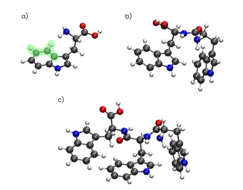
Figure 2: Molecular structure of tryptophan and its derivatives: a) monomer with the fragment used to compare different embedding approaches indicated in green, b) dimer, and c) trimer. Carbon atoms are indicated in black, hydrogen atoms in white, oxygen atoms in red, and nitrogen atoms in blue.

Although our results are specific to the examples chosen, we expect their electronic structures to be representative for a more general picture of electronic states. This is due to the regular structure of the amino-acid building blocks of proteins. The results obtained for tryptophan and its oligopeptides will be easily transferable to the homologous and also aromatic amino acid phenyl alanine and may be straightforwardly generalized to the other essential amino acids.

We first applied a density-matrix based embedding. Specifically, we used the bootstrap embedding algorithm for molecular systems [38] on a selected five-atom fragment that is part of the aromatic side chain, depicted in Fig. 2. This fragment was selected as it represents an intuitively challenging embedded system, as it is connected to the environment with both single and delocalized conjugate double bonds. For the bootstrap embedding, a set of orthogonal localized orbitals was constructed using the intrinsic atomic orbitals scheme [73]. This basis was then used to perform the Schmidt decomposition of the HF state and select the set of fragment and entangled bath orbitals. Fragment orbitals selected in this way were localized on atoms, making them a poor choice for the wavefunction representation. Therefore, the selected fragment and bath orbitals were transformed to the eigenvectors of the Fock operator in the fragment-bath space, resulting in canonical orbitals depicted in Fig. 3 a). Due to the nature of Schmidt decomposition, these orbitals resemble the canonical HF orbitals of the entire system and, consequently, exhibit relatively small single-orbital entropies (defined as von Neumann entropies of the one-orbital reduced density matrix [61]). Hence, the multiconfigurational character of the fragment-bath system obtained with bootstrap embedding is comparable to the one of the entire system, even though fragmentation ‘cuts’ through single and double bonds (Fig. 3 b)). From the drop in the values of the single-orbital entropies one can conclude that there are twelve orbitals that contribute the most to the multiconfigurational character and the static correlation [64, 74] and include the reconstructed delocalized aromatic $\pi$ system of the side chain (Fig. 3). Note that in the complete bootstrap embedding, one would apply this construction to multiple fragments, and then perform a matching procedure between the different fragments, a step we ignore for the purpose of this discussion.

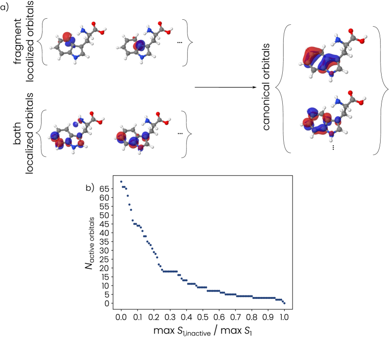
Figure 3: a) Left: fragment and bath orbitals obtained from the Schmidt decomposition of the HF state, Right: canonical orbitals obtained from the HF calculation in the fragment-bath space. b) Threshold diagrams corresponding to the maximal discarded single-orbital entropies relative to the largest value ($\text{max}\ S_{1}=0.19115$) for different active space sizes, as introduced in Ref. [64].

Next, we performed DMRG calculations for different active space sizes in the fragment-bath space, with orbitals being selected based on the largest values of the single-orbital entropies, as described in Ref. [64]. We use a bond dimension of $D=1024$ to yield a reference MPS that can be taken as a reliable approximation to the exact (full configuraion interaction, or FCI) ground state. To assess the suitability of MPS wavefunctions with smaller bond dimensions for initial state preparation, we calculate both energy differences and overlaps of them with the reference MPS; the results are shown in Fig. 4 a) and b).

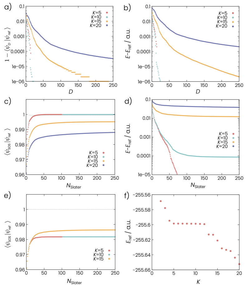
Figure 4: a) Overlap of truncated MPS wavefunctions with the reference MPS of bond dimension $D=1024$ (taken as an approximate FCI result) for different active space sizes $K$. b) Corresponding energy differences of the small-bond-dimension and the reference MPS. c) Overlap of sum-of-Slater states with different numbers of Slater determinants with the reference MPS wavefunction d) Corresponding energy differences of the sum-of-Slater states and reference MPS state e) Overlap of sum-of-Slater states obtained from reference MPS wavefunctions in smaller active orbital spaces with the reference MPS wavefunction of the largest active space considered ($K=20$) f) Reference MPS energies for different active space sizes

From Fig. 4 one can see that the overlap of the truncated states with the reference MPS state approaches a value of one relatively quickly. This is expected, as the truncation of the bond dimension is performed in the optimal way using the singular value decomposition, selecting the state of the lower bond dimension that has maximal overlap with the nontruncated one. For similar reasons, the energies of the small-bond-dimension states quickly approach the corresponding reference energy. Furthermore, even states with bond dimension $D=2$ already demonstrate excellent overlap with the reference MPS state ($\approx 0.97$), making such an MPS a good candidate for state preparation.

We also consider a different ansatz, namely sum-of-Slater states (see Appendix A and [9] for a discussion of such states on quantum computers). We obtain these by selecting the most important determinants from the FCI-type expansion represented by the reference MPS wavefunction, keeping the $N_{\text{Slater}}=L$ terms with the largest amplitudes:

$$\ket{\Psi_{\text{SOS}}}=\frac{1}{\sqrt{\sum_{i=1}^{L}\absolutevalue{C_{i}}^{2}}}\sum_{i=1}^{L}C_{i}\ket{\Phi_{i}}$$ (2)

where $\ket{\Phi_{i}}$ are Slater determinants in a fixed basis of orbitals, and we have ordered so $\absolutevalue{C_{1}}\geq\absolutevalue{C_{2}}\geq\dots$. These states are both useful as a guiding state Ansatz (for small $L$), and to understand the correlation structure of the ground state. From Fig. 4 c), it can clearly be seen that the overlap obtained for these sum-of-Slater expansions with the reference MPS wavefunction are again relatively large. However, convergence of these overlaps with the number of included determinants is much slower than the convergence of small-bond-dimension MPS wavefunctions with increasing bond dimension. Moreover, convergence is slowed down even further for increasing active space sizes $K$, which may be taken as an indication of the orthogonality catastrophe in the large active space limit. It is thus necessary to weigh both the gate count for the preparation of MPS and sum-of-Slater states and the quality of the overlap that they provide for the specific system of interest.

With respect to the correlation structure of the ground state, it is noteworthy that the change of overlap exhibits two different regimes, with a large jump at a small number of Slater determinants, followed by a slow convergence to unity. The initial jump corresponds to the inclusion of the Slater determinants describing excitations into the virtual orbitals with the largest values of the single-orbital entropies, which carry the largest coefficients in the FCI expansion and account for static correlation. Although overlaps with the reference MPS wavefunction are comparatively large, energies corresponding to the sum-of-Slater states converge slowly to the reference MPS energy (Fig. 4 d)). Such behavior is expected, as truncation of a Slater-determinant expansion results in a neglect of a significant portion of the dynamical correlation energy. By contrast, an MPS, even if truncated to very low bond dimension, can represent a large number of Slater determinants, resulting in much better convergence behavior, which makes them a good candidate for guiding states with high ground state overlap [9].

We now investigate the quality of the sum-of-Slater states obtained for smaller active spaces as initial states for the larger active space ($K=20$). As can be seen in Fig. 4 e), the sum-of-Slater ansatz prepared in an active space with $K=15$ orbitals provides overlaps that are virtually indistinguishable from the reference. In the case of $K=5$ and $K=10$, the overlap is somewhat lower when compared to the sum-of-Slater state prepared in the $K=15$ case, but still represents an improvement over the Hartree-Fock state. This is due to the fact that not all highly entangled orbitals are included in these cases (as can be seen from the Fig. 3 b)), resulting in a lack of several determinants with non-negligible coefficients. However, it can be seen that as long as the most entangled orbitals are included, these active spaces provide sum-of-Slater states that are of the same quality in terms of overlap as the ones obtained from the calculation on the larger active space.

Finally, from the Fig. 4 f), it is evident that many orbitals must be considered to reach chemical accuracy in absolute energies, as they carry a significant portion of the correlation energy. The fact that the initial state can be prepared in smaller active spaces therefore significantly reduces the computational overhead for the classical part of the initial state preparation.

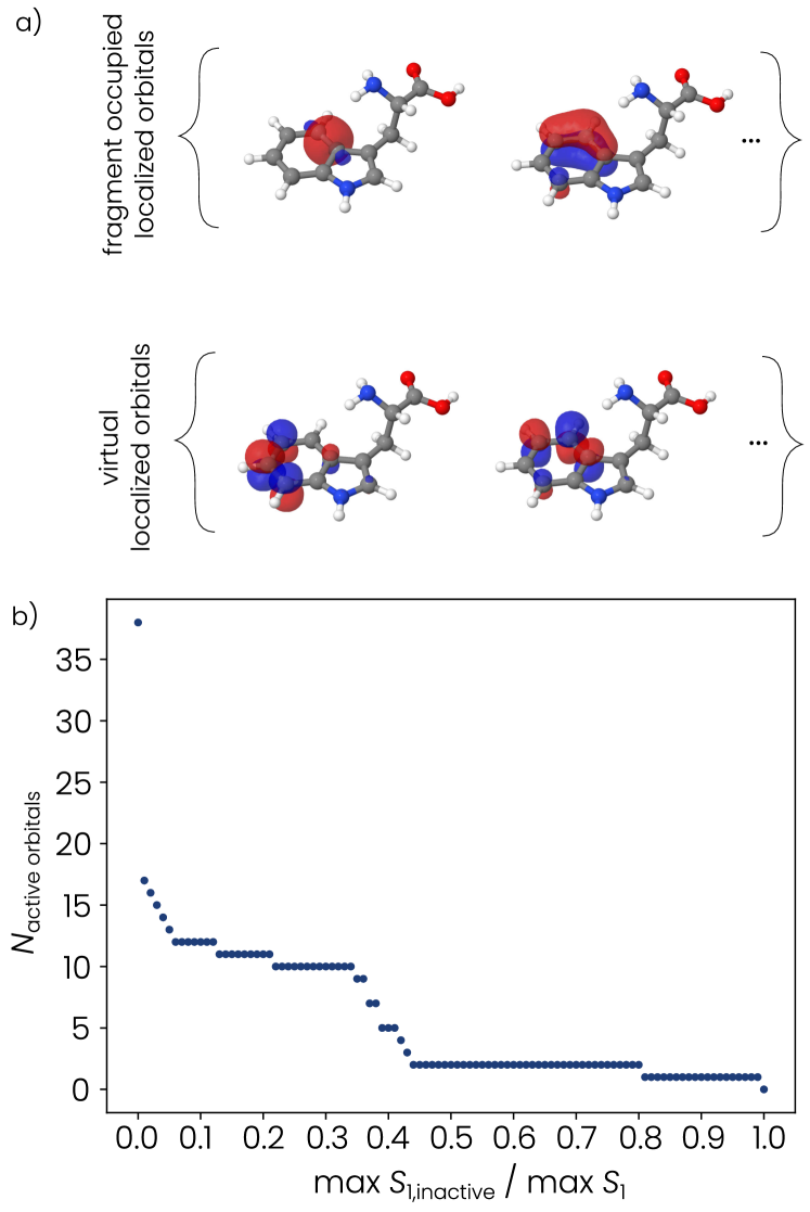
Figure 5: a) Localized occupied fragment orbitals and localized virtual orbitals obtained in Huzinaga embedding c) Threshold diagrams corresponding to the maximal discarded single-orbital entropies relative to the largest value ($\text{max}\ S_{1}=0.21866$) for different active space sizes, as introduced in Ref. [64]. This may be contrasted with Fig. 3.

We also investigated a projection-based Huzinaga embedding [39, 75], using the same five-atom fragment, in order to assess how different embedding strategies affect the state preparation problem. There are several key differences with respect to bootstrap embedding. Firstly, the orbitals used for the Huzinaga embedding are obtained from a DFT calculation on the entire molecule, while the basis for the density-matrix approach in the bootstrap embedding is a HF calculation. This results in a different Hilbert space for the fragment problem. Secondly, in the Huzinaga embedding, interaction of the fragment orbitals with the occupied environment is described with a DFT potential, which approximates the correlation contributions from the occupied environment orbitals that are neglected in the case of bootstrap embedding. This interaction modifies the one-electron part of the fragment Hamiltonian. Third, a split orbital localization scheme is applied within the Huzinaga embedding, based on intrinsic bond orbitals [73, 76], while canonical orbitals are used in the bootstrap embedding, which results in a qualitatively different multiconfigurational character of the fragment wavefunction in these cases. Unlike bootstrap embedding, the entire virtual space is considered in Huzinaga embedding and the canonical orbitals are not recomputed after the embedding. Due to the local nature of the orbitals, the values of the single-orbital entropies are significantly different from the bootstrap embedding case (Fig. 5 and Fig. 3). In Huzinaga embedding, orbital entropies are larger when compared to the bootstrap case, which can be attributed to the usage of localized orbitals [77]. This results in a larger number of highly entangled orbitals, while the contribution of the virtuals that are spatially separated from the embedded fragment decreases significantly.

Due to the small entanglement of some virtual orbitals, convergence of the sum-of-Slater states both in terms of overlap and energy is faster than in the bootstrap embedding case (Fig. 6 a) and b)). Hence, localized orbitals might present a more suitable basis for initial state preparation. Whereas one In classical quantum chemical methods one aims for a pronounced single-configurational character of the wavefunction and accounts for dynamic correlation a posteriori. In contrast, for quantum computers, it may be more desirable to have a multiconfigurational wavefunction with little residual dynamic correlation (Fig. 6 d)), since given a guiding state with only constant overlap, phase estimation gives accurate energies on the fragment orbitals. Similar to our bootstrap embedding results, initial states with large overlap can be prepared in a smaller active space, reducing the cost of a classical calculation for the state preparation step also in the case of Huzinaga embedding (Fig. 6 c)).

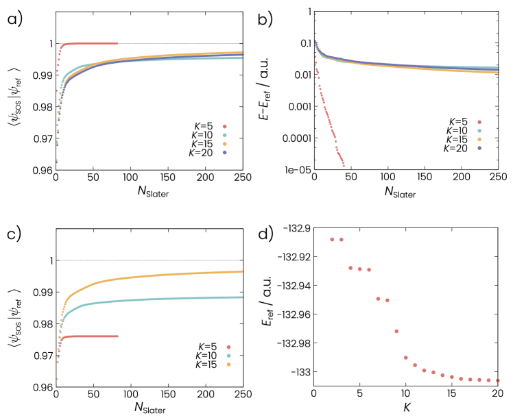
Figure 6: a) Overlap of sum-of-Slater states (with $N_{\text{Slater}}$ Slater determinants corresponding to the largest coefficients) with the reference MPS state of bond dimension $D=1024$ for different active space sizes $K$. b) Overlap of sum-of-Slater states for different active space sizes $K$ with the reference MPS state ($D=1024$) for the largest active space considered $K=20$. c) Energies of sum-of-Slater states, with lines corresponding to the energies of the full MPS wavefunction. d) Energy of the MPS ground state energy approximation, as a function of active space size $K$.

Finally, we turn to the sequence of tryptophan molecules mimicking an oligopeptide structure. We chose the active spaces to be residing entirely on the side chain (see Appendix D for details). First, we consider the limit of noninteracting side chains corresponding to separated tryptophan molecules in the sequence. In this case, the overlaps of the HF state with the reference MPS states decay exponentially with the number of tryptophan molecules (Fig. 7 a)). In the case of sum-of-Slater states, the decay is approximately exponential as well. The exact exponential dependence occurs when the Slater determinants included correspond to the wavefunction that is a product of sum-of-Slater states on each monomer. Since the monomer ground state has relatively high overlap with the HF state, we see that the overlap of the HF state is still substantial (at around 0.7) for a sequence of 5 tryptophane molecules.

We also compute the overlap with the ground state of the interacting tryptophan dimer and trimer. It can be seen that weak interactions (between the side chains) only marginally perturb the overlap behavior observed for the separately treated side chains, so the exponential decay from the non-interacting case is a good approximation. We performed embedding calculations for a single side chain in ditryptophan (at the C-terminus side chain) and tritryptophan (side chain at the amino acid in the middle) and investigated the resulting overlaps of the sum-of-Slater states. As can be seen in Fig. 7 b), the behavior of the overlap in both cases of the embedded monomers is essentially the same as in the case of a single tryptophan side chain. From these observations, we may conclude for proteins that embedding of relevant amino acid side chains represents a good strategy for mitigation of the orthogonality catastrophe caused by large system size.

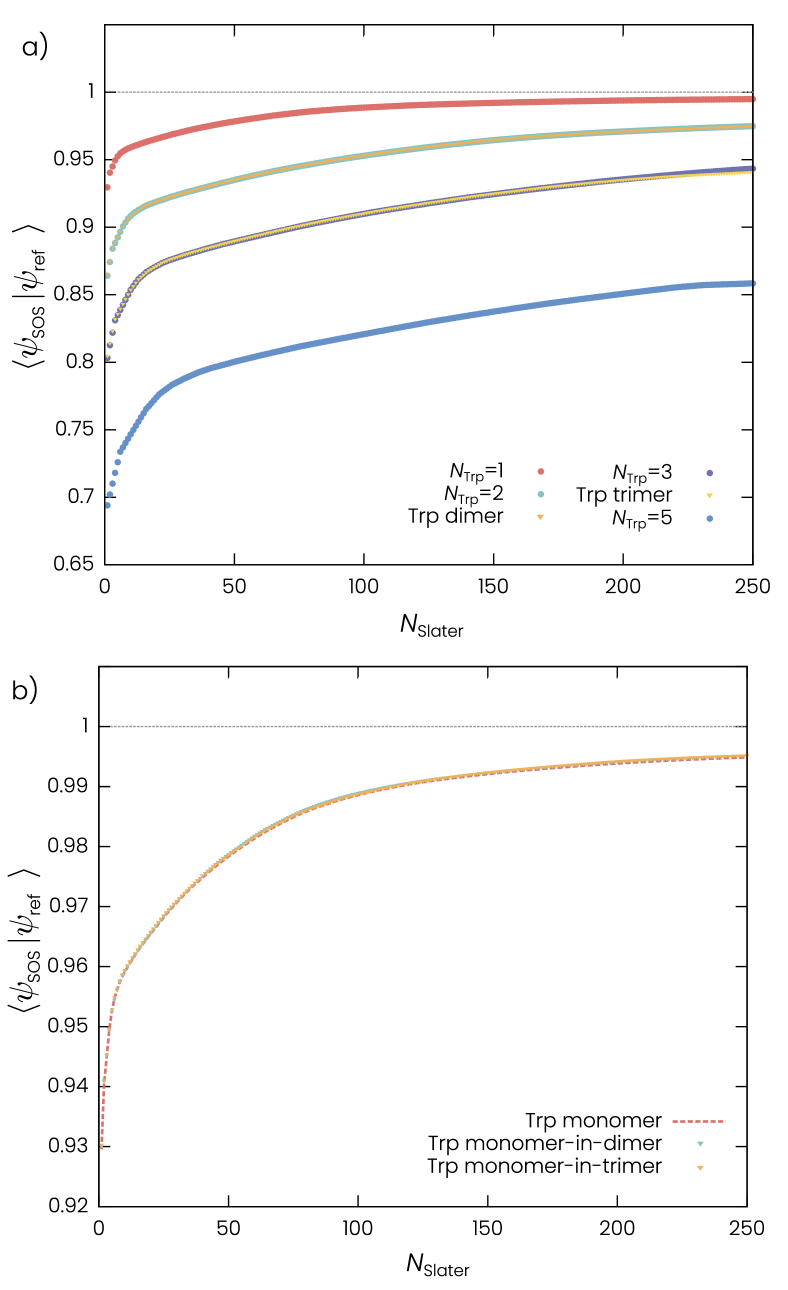
Figure 7: a) Overlap of sum-of-Slater states containing $N_{\text{Slater}}$ Slater determinants with the with the reference MPS state of bond dimension $D=1024$ for different numbers of noninteracting tryptophan residues (circles) and interacting residues in ditryptophan and tritryptophan (triangles, note: the data for the interacting dimer and trimer overlaps with the data for the noninteracting cases) b) Same as a) for a single monomer embedded into the ditryptophan and tritryptophan (triangles). Values for the isolated monomer are given as a dashed line.

IV.2 Ruthenium anti-cancer drug

As a second example, we consider a system containing elements beyond the second period of the periodic table. This compound (see Fig. 8 for a ball-and-stick representation of its structure) is an anti-cancer drug [78, 79] which can bind as an inhibitor to a glucose-regulating protein [80]. Such a binding is a typical example of small-molecule drug recognition by biomacromolecules and therefore an example for a molecular recognition application. Here, we focus on the isolated Ru-based drug molecule and consider its central region, the Ru ion containing moiety, as a quantum core (as highlighted in green in Fig. 8). We leave an investigation of how the ground state overlap problem changes when including the target protein in the embedding to future work.

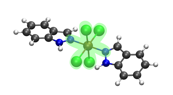
Figure 8: Molecular structure of the ruthenium complex with the fragment used for the Huzinaga embedding indicated in transparent green. Carbon atoms are indicated in black, hydrogen atoms in white, nitrogen atoms in blue, chlorine atoms in green, and the ruthenium atom in brown.

For this complex, we applied the Huzinaga embedding of the ruthenium ion and its first (nearest-neighbor) coordination sphere (Fig. 8). We consider two different charges of this complex: the anion, $q=-1$, corresponds to a doublet state, and the neutral complex, $q=0$, we considered as a triplet ground state. For the doublet, the overlap of HF state and the sum-of-Slater states is very large, indicating a single-configurational character of the wavefunction. By contrast, the triplet state exhibits smaller overlap of the HF determinant with the reference MPS state of bond dimension $D=1024$, which is quickly cured by including a second Slater determinant to yield a large overlap, see Fig. 9. This behavior is a consequence of the triplet nature of the wavefunction, which cannot be described by a single spin-restricted determinant. However, it can be described with a configuration state function which is a symmetry-adjusted basis state. In the case of the triplet, the configuration state function is a linear combination of two restricted Slater determinants (and therefor multi-configurational). If the system of interest is comprised of several high-spin regions with (e.g., in the case of metal clusters), the overlap of the HF determinant will further decrease, depending on the number and spins of these regions [13]. It has already been argued that spin coupling to produce configuration state functions effectively solves this problem [15]. However, we note that such situations are not at all common in biomolecular recognition situations.

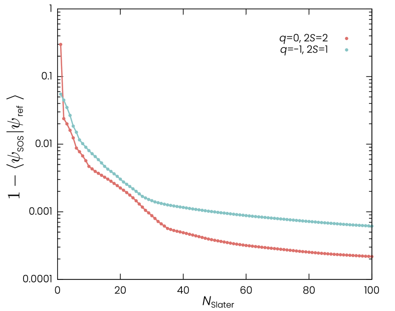
Figure 9: Overlap of sum-of-Slater states (with $N_{\text{Slater}}$ Slater determinants corresponding to the largest coefficients) with a reference MPS state of bond dimension $D=1024$ for the doublet (net charge $q=-1$) and triplet (net charge $q=0$) electronic states of the embedded fragment in the ruthenium complex.

V Conclusions

In this work, we have demonstrated that embedding methods effectively solve the orthogonality catastrophe in practice for problems with local spatial structures, specifically in biochemistry. We show that for two conceptually different quantum embedding methods, low complexity states serve as good guiding states for quantum phase estimation. We demonstrate this is the case for the fundamental building blocks of biomolecules, but also for other compounds such as small metal-containing drug molecules. As expected, the ground state overlap of the mean-field HF basis state with the target state decreases with increasing active space size, but based on our estimates, phase estimation will likely face bottlenecks due to the polynomial scaling of simulation methods with the number of orbitals $N$ before small or vanishing ground state overlaps become problematic. This is clearly a positive prospect for quantum algorithms for ground state energy estimation, especially for biochemical applications.

For general applicability, we have also studied embedding and guiding state preparation for impurity models. Here we argued for the existence of accurate small active orbital spaces and for mild scaling of ground state overlap. An interesting open question is whether the quantum impurity problem without any further restrictions is in BQP. The mathematical analysis of embedding methods and of quantum impurity problems is based on the natural occupation numbers of the 1-RDM. Future work could explore whether the structure of 1-RDMs, which satisfy additional linear constraints [81, 82], can be used to improve quantum embedding schemes [83, 84, 85] and help to find good guiding states for phase estimation.

Various interesting challenges remain to assess the utility of fault-tolerant quantum computers for ground state energy estimation of electronic structure in chemistry. As we have emphasized, one of the main advantages of quantum computing based on phase estimation over conventional methods are its accuracy guarantees. However, embedding methods introduce an (uncontrolled) error, even if small in practice. A better understanding of this error and the effect of the approximate treatment of the environment on the quantum core will be important for applications of quantum computers to macromolecules and requires further work.

Appendix A Guiding states in quantum chemistry

This appendix contains a review of the guiding state problem for quantum chemistry. We start by briefly reviewing the dependence of quantum phase estimation on the ground state overlap of the guiding state. Next we give an overview of different ansatzes for guiding states. We discuss different types of correlation in quantum chemistry, and why one expects that the ground state overlap vanishes exponentially for increasing system size (the orthogonality catastrophe).

A.1 Quantum circuits and guiding state preparation

To estimate the ground state energy one would like to apply quantum phase estimation with the time-evolution operator $U(t)=\exp(itH)$. Then, using a guiding state $\ket{\psi}$ with ground state overlap $\absolutevalue{\braket{\psi}{\psi_{0}}}\geq\eta$, one finds an approximation to the ground state energy with probability $\eta^{2}$. Therefore, the ground state overlap is related to the number of repetitions needed to find the ground state energy through phase estimation. An approximation of accuracy $\varepsilon$ requires a circuit with time evolution for time $\mathcal{O}(\varepsilon^{-1})$, leading to a total cost of $\tilde{\mathcal{O}}(\varepsilon^{-1}\eta^{-2})$. The scaling with $\varepsilon^{-1}$ is known as Heisenberg scaling and is optimal [86], but different approaches to phase estimation have different scalings with the ground state overlap. Given access to a quantum circuit preparing $\ket{\psi}$, one can find the ground state energy using $\mathcal{O}(\eta^{-1})$ uses of this state preparation unitary, and time evolution for time $\tilde{\mathcal{O}}(\varepsilon^{-1}\eta^{-1})$. This scaling is optimal [87] but does, however, lead to deeper circuits. On the other hand, there are also approaches which only require a single ancilla qubit and time evolution for time $\tilde{\mathcal{O}}(\varepsilon^{-1})$ [88]; these require $\tilde{\mathcal{O}}(\eta^{-4})$ circuit repetitions. Finally, in the regime where $\eta\to 1$ it is possible to reduce the maximal circuit depth, at the cost of an increased number of repetitions. If $\delta=1-\eta^{2}$, the maximal required time evolution can be reduced to $\mathcal{O}(\delta\varepsilon^{-1})$, with a total evolution time of $\mathcal{O}(\delta\varepsilon^{-2})$ [16, 17]. This means that if one can find guiding states with ground state overlap surpassing $\eta\geq 0.9$ using cheap conventional methods, this may be used to signifificantly reduce the required circuit depth for accurate energy estimates using quantum phase estimation, which may be helpful for realizing such simulations on devices with limited number of qubits and maximal circuit depth.

There are three standard classes of guiding states for chemistry problems, which we will now briefly review, together with the cost of preparing them on a quantum computer. We refer to [9] for an extensive overview. For convenience we assume we are using a Jordan-Wigner mapping for the fermion-to-qubit mapping of the electronic structure problem. We quote the best known gate counts for two measures: the number of two-qubit gates required (and ignoring the number of single-qubit gates); or alternatively the number of Toffoli gates (and ignoring the number of Clifford gates). The first measure is relevant for current and near-term devices where two-qubit gates are typically much slower and more noisy than single-qubit gates. The second measure applies to a fault-tolerant model where the main cost comes from the non-transversal (non-Clifford) operations.

1. Single Slater determinant: This is the most basic case. Hartree-Fock yields a single Slater determinant, and under a fermion-to-qubit mapping this state is represented by a product state (which requires no two-qubit gates or $T$ gates to prepare). If we use the standard Jordan-Wigner mapping with canonical orbitals (compatible with the HF state), then for $N$ spin-orbitals and $n$ electrons this is simply the state $\ket{1}^{n}\ket{0}^{N-n}$. It is also possible to choose a single Slater determinant in a different orbital basis than the one used for the fermion-to-qubit mapping, which can significantly improve the ground state overlap [8, 14]. A single-particle basis change can be implemented as a quantum circuit using so-called Givens rotations. Using the Jordan-Wigner representation, this requires $n(N-n)$ two-qubit gates [89].

2. Sum-of-Slater determinants: A direct extension is to take a state which is a superposition of a (small) number $L$ of Slater determinants, as in Eq. 2. Such states can for example be found through configuration interaction with single and double excitations (CISD) methods or selective configuration interaction (SCI) methods [9]. Alternatively, they can be extracted as the dominant coefficients of a matrix product state (see below). Again, if we assume that the fermion-to-qubit mapping uses the same orbital basis, such states are mapped to a superposition of $L$ standard basis states. These can be prepared using at most $\mathcal{O}(NL)$ two-qubit gates, see [90] for explicit gate counts; or $\mathcal{O}(L\log(L))$ Toffoli gates and $\big{(}\log(L))$ ancilla qubits [9]. Additionally, if the number of excitations from the HF state is bounded by $k$, $\mathcal{O}(Lk)$ two-qubit gates suffice [91].

3. Matrix product states: A final power class of states are matrix product states (MPS). These can be found using the density matrix renormalization group (DMRG) algorithm and are characterized by their bond dimension $D$. Accurate quantum chemistry calculations typically require a large bond dimension, but alternatively one can either try to minimize over low bond dimension MPS, or truncate a high bond dimension MPS to a low bond dimension state which has less accurate energy but still significant ground state energy overlap. In many cases, this leads to high-quality guiding states [9], but at a relatively high classical processing cost. MPS can be prepared in sequential fashion, using $\mathcal{O}(ND^{2})$ gates (either two-qubit or Toffoli) [92] and depth scaling with $N$. Heuristic methods for short depth circuits preparing states with high overlap with a given MPS can be found in [93, 94]. Other depth reduction techniques are based on the correlation length of the MPS [95], or by using mid-circuit measurements and adaptive circuits [96].

Other methods for finding and preparing guiding states, not discussed in this work, include adiabatic state preparation [97, 98], thermal state preparation algorithms [99] and variational approaches based on unitary coupled cluster methods [100].

A.2 The orthogonality catastrophe

In most cases in many-body physics, requiring approximations at the level of the wavefunction which are such that they have large overlap with the true ground state is a very strong requirement. As we will explain below in more detail, small (local) errors in the approximation leads to essentially orthogonal states on the many-body level, a phenomenon known as the orthogonality catastrophe. Nevertheless, for quantum algorithms it is in fact important to prepare guiding states which have a significant overlap with the true many-body ground state in order to guarantee that the quantum phase estimation algorithm will give a good estimate of the ground state energy.

We collect four basic arguments for the orthogonality catastrophe, based on accumulation of error and Andersons impurity argument in the thermodynamic limit, the electron-electron cusp in the continuum limit, and finally an argument from the computational complexity of the ground state problem.

The most basic intuition for the orthogonality catastrophe is that if we have an extended system consisting of $N$ subsystems without any correlation between the systems, the global ground state overlap decays exponentially if there is a local approximation error. If the true state is $\ket{\phi}^{\otimes n}$, and we have on-site estimates $\ket{\psi}$ of $\ket{\phi}$, then the global squared overlap decays exponentially as $\absolutevalue{\braket{\phi}{\psi}}^{2N}$ (and the same is true for uncorrelated fermionic systems) [101]. While this gives a reasonable intuition, it is also a very artificial scenario.

In [55] Anderson showed that a similar phenomenon occurs for a realistic physical system of an electron gas with an impurity. The impurity is a local sized perturbation, which is constant-sized compared to the number of electrons. The ground state of the perturbed system has an overlap with the ground state of the unperturbed system which, in this case, decays polynomially with the system size. Note that this differs from the uncorrelated example, where the decay arises from the fact that every local fragment incurs an error. This phenomenon is known as the Anderson orthogonality catastrophe. This can be derived in perturbation theory for a one-body perturbation [55]. This means that for impurity models, the orthogonality ‘catastrophe’ may only be of polynomial nature and therefore need not be an obstruction to an efficient quantum algorithm as one may hope that the ground state has a polynomially decaying overlap with the mean-field state. We partially make this idea rigorous in Section III and Appendix C, based on the work of [21].

Another fundamental reason for the orthogonality catastrophe lies in the continuum limit rather than the thermodynamic limit. Here we keep the number of electrons $n$ fixed, but increase the spatial resolution of the second-quantized Hamiltonian by raising the number of orbitals $N$. This leads to convergence to the true wavefunction in $L^{2}(\mathbb{R}^{3n})\otimes\mathbb{C}^{2}$. Note that the Hilbert space of a fixed number of electrons $n$ but increasing $N$ scales polynomially (but with an exponent scaling with $n$). It is well known that resolving the electron-electron cusp of the wavefunction of any system with Coulomb interactions requires a diverging number of Slater determinants (see for example the discussion in Chapter 7 of [7]). This is well understood analytically [102, 103, 104], and is true for arbitrary eigenfunctions of the electronic structure Hamiltonian. In particular, it is known that the 1-RDM in the continuum limit has eigenvalues (i.e. natural occupation numbers) decaying as $\lambda_{k}\sim k^{-\frac{8}{3}}$ as $k$ goes to infinity [102], lower bounding the required number of (natural) orbitals needed to approximate the exact wavefunction.

A final argument for a version of the orthogonality catastrophe comes from complexity theory. The problem of computing ground state energies is known to be QMA-complete, which means that it is strongly believed to be hard for quantum computers. This remains true in the case of electronic structure Hamiltonians [65, 12]. As a result, there should be no efficient (quantum) algorithm for finding states with at most polynomially decaying overlap with the true ground state: if such an algorithm existed, it could be used to prepare an initial state for the quantum phase estimation algorithm and thus efficiently estimate the ground state energy. On the other hand, it is known that the ground state estimation problem remains BQP-hard even if one is provided a guiding state with very high ground state overlap [105]. This means that in general, having classical methods which achieve reasonable overlap does not imply the ability to improve this precision arbitrarily in an efficient manner (although this could still be the case in practice for problems in chemistry, as suggested by [13]).

Finally, for the general class of Hamiltonians which have an (unknown) efficiently describable guiding state whose expectation values can be computed efficiently using a classical computer (such as MPS), the ground state energy problem is QCMA complete [106]. This provides evidence that in general guiding states which can efficiently be described classically may still be hard to find.

A.3 Guiding states in chemistry

Electronic structure theory is the main quantum mechanical problem in chemical and materials science. We distinguish three regimes:

1. The weak correlation limit: In the weak correlation limit the mean-field Hartree-Fock state is already an excellent qualitative approximation. As discussed, these are easy to prepare on a quantum computer, and this suffices as the choice of guiding state. Most chemical processes belong to this class. However, for these systems coupled cluster models based on a Hartree-Fock reference state deliver reliable results because they can efficiently account for the lacking dynamic correlation (yet, with unknown system-focused error for a specific application [18]). Small molecule [8] belong to this class, as well as electronic host-guest binding energy calculations such as those required in drug design problems. Quantum computers potentially exhibit an advantage in this regime for larger numbers of orbitals $N$. Then, quantum phase estimation can, in principle, obtain an energy of guaranteed accuracy that can be taken as a reference for standard coupled cluster models.

2. The intermediate correlation limit: Here, static electron correlation can become important and multi-configurational approaches are more suitable. In this regime, traditional computation begins to face severe problems. Only coupled cluster models that can deal with a multi-configurational reference or that are of high excitation degree (including at least quadruple excitations) are applicable. However, the former are not unambiguously defined, whereas the latter are too costly for all but the smallest molecules. At the same time, generic multi-configurational models such as the complete active space self-consistent field (CASSCF) wavefunction and the MPS wavefunction optimized by DMRG are natural choices, but suffer from a lack of similarly accurate dynamical correlation methods to account for the fact that CASSCF and DMRG approaches are restricted to a few dozens of orbitals only. Nevertheless, only a small number of determinants (say, on the order of a dozen) will represent the state qualitatively well. Their superposition can be initialized efficiently as a guiding state on a quantum computer (provided that knowledge about these determinants can be obtained at comparatively little cost before a quantum computation).

3. The strong correlation limit: A large number of Slater determinants will be required in order to achieve a sufficiently high overlap with the target state. There are only few examples known in ground-state chemistry of this kind. A prominent class of examples are iron-sulfur clusters, where the overlap of the optimal Slater determinant with the ground state becomes very small [13], while DMRG optimized MPS may still have large overlap. Such cases can be more routinely found in materials science, where materials are built from many units with half-filled single-particle states, or in electronically excited states.

Generally, to assess the quantum advantage of quantum phase estimation, a better understanding of which systems have polynomially scaling conventional methods in practice on the one hand, and an understanding of which systems allow for good guiding states is required [13, 9].

Appendix B Fermionic formalism

We start by defining notation and recalling the formalism of fermionic quantum systems. We consider a single-particle space $\mathcal{H}$ of dimension $N$ which we may identify with $\mathbb{C}^{N}$. We refer to elements of the single-particle space $\mathcal{H}$ as modes; or equivalently in chemistry terminology as orbitals. The full Hilbert space is the Fock space

$$\bigoplus_{n=0}^{N}\mathcal{H}^{\wedge n}\cong(\mathbb{C}^{2})^{\otimes N}$$

which can be mapped to $N$ qubits. Numbering an orthonormal basis of modes $j=1,2,\dots,N$, we associate creation and annihilation operators $a_{j}$ and $a_{j}^{\dagger}$ respectively which satisfy the fermionic anticommutation relations

$$\{a_{j},a_{k}\}=0=\{a_{j}^{\dagger},a_{k}^{\dagger}\}\ ,\quad\{a_{j},a_{k}^{\dagger}\}=\delta_{jk}\ .$$

We define the vacuum state $\ket{\Omega}$ to be the unique mutual kernel of all the operators $a_{j}$, from which the creation operators $a_{j}^{\dagger}$ generate the full Hilbert space as a Fock space. Given any normalised vector $x=(x_{1},\dots,x_{N})\in\mathbb{C}^{N}$ we let

$$a^{\dagger}(x)=\sum_{j=1}^{N}x_{j}a_{j}^{\dagger}\qquad a(x)=\sum_{j=1}^{N}\overline{x_{j}}a_{j},$$

be the operators which create and annihilate the mode $x$.

The operators

$$\hat{n}(x)=a^{\dagger}(x)a(x)\qquad\hat{n}=\sum_{j=1}^{N}a_{j}^{\dagger}a_{j}$$

are the number operator for mode $x$ and the total number operator. If $\ket{\Psi}$ is an eigenvector of $\hat{n}(x)$ with eigenvalue 0 or 1 we say that mode $x$ is respectively unoccupied or occupied in the state $\ket{\Psi}$. Given a state $\ket{\Psi}$, its covariance matrix or one-body reduced density matrix (1-RDM) is operator on $\mathcal{H}$ defined by

$$\langle x,\gamma y\rangle=\bra{\Psi}a^{\dagger}(x)a(y)\ket{\Psi}.$$

After a choice of basis this gives an $N\times N$ matrix with entries $\gamma_{jk}=\bra{\Psi}a_{j}^{\dagger}a_{k}\ket{\Psi}$.

A Slater determinant is a state of the form

$$a^{\dagger}(x_{n})\dots a^{\dagger}(x_{1})\ket{\Omega}$$

where $x_{1},\dots,x_{n}$ are a collection of orthonormal modes in $\mathcal{H}$. Up to a phase, the Slater determinant only depends on the subspace $\mathcal{X}$ spanned by the $x_{i}$, and it is the state where the modes in $\mathcal{X}$ are occupied, and the modes in $\mathcal{X}^{\perp}$ are unoccupied.

We can also define the $2N$ Majorana operators

$$c_{2j-1}=a_{j}+a_{j}^{\dagger}\qquad c_{2j}=-i(a_{j}-a_{j}^{\dagger}).$$

A Gaussian unitary is a unitary $U$ acting on the Fock space such that as an orthogonal transformation $O\in O(2N)$,

$$Uc_{p}U^{\dagger}=\sum_{q}O_{pq}c_{q}\ .$$

for an orthogonal transformation $O\in O(2N)$. A Gaussian state is a state of the form $U\ket{\Omega}$, where $U$ is a Gaussian unitary operator. In particular, any Slater determinant is a Gaussian state.

A non-interacting (or free, or one-body) Hamiltonian is a Hamiltonian of the form

$$H_{\operatorname{free}}=\sum_{j,k}h_{jk}a_{j}^{\dagger}a_{k}$$

where $h$ is a Hermitian operator on $\mathcal{H}$. By choosing a basis for $\mathcal{H}$ in which $h$ is diagonal, we can always transform this to the form

$$H_{\operatorname{free}}=\sum_{j=1}^{N}\epsilon_{j}\tilde{a}_{j}^{\dagger}\tilde{a}_{j}$$

with $\epsilon_{1}\leq\epsilon_{2}\leq\dots$. The ground state space of a non-interacting Hamiltonian is spanned by a set of Slater determinants. If $\epsilon_{j}<0$ for $j\leq n$, and $\epsilon_{j}>0$ for $j>n+k$, then the ground state space is spanned by the set of Slater determinants for which modes $1,\dots,n$ are occupied and $n+k,\dots,N$ are unoccupied. In particular, if $\epsilon_{j}\neq 0$ for all $j$ then the ground state is unique.

In this work we are concerned with quantum impurity Hamiltonians, where a free Hamiltonian is perturbed by a non-negligible but spatially localised impurity term $H_{\operatorname{imp}}$. The term $H_{\operatorname{imp}}$ is localised in the sense that, written in terms of the fermionic operators $a_{j}$, $a_{j}^{\dagger}$, it only contains the modes $j\leq M$ for some constant $M$.

Definition B.1.

A quantum impurity Hamiltonian is a Hamiltonian of the form

$$H=H_{\operatorname{free}}+H_{\operatorname{imp}}.$$

where $H_{\operatorname{free}}$ is a non-interacting Hamiltonian on $N$ modes, and $H_{\operatorname{imp}}$ is an interacting Hamiltonian a subset of $M$ of the modes. The quantum impurity problem is the problem of computing the ground state energy of $H=H_{\operatorname{free}}+H_{\operatorname{imp}}$ to accuracy $\varepsilon$, where $H_{\operatorname{free}}$ has bounded single-particle energies $\epsilon_{j}$.

In this computational problem, note that $H_{\operatorname{imp}}$ and $M$ are taken to as constant parameters: we seek an efficient solution in terms of the total system size $N$ and the precision $\varepsilon$.

There are a few ways in which this problem can be simplified. Firstly, note that we can without loss of generality assume that the single-particle energies are non-negative. This follows by defining a new set of fermionic operators $b_{j}$ by

$$b_{j}=\tilde{a}_{j}^{\dagger}\qquad \text{ for }j=1,\dots,n$$

$$b_{j}=\tilde{a}_{j}\qquad \text{ for }j=n+1,\dots,N\ ,$$

where $n$ is maximal such that $\epsilon_{n}<0$, as above. More generally, this corresponds to the transformation

$$b(x)=\sum_{j=1}^{n}x_{j}a_{j}^{\dagger}+\sum_{j=n+1}^{N}\overline{x_{j}}a_{j}\ .$$

Under this transformation, the free Hamiltonian takes the form (after a constant energy shift)

$$H_{\operatorname{free}}=\sum_{j=1}^{N}\absolutevalue{\epsilon_{j}}b_{j}^{\dagger}b_{j}\ ,$$

and the state vacuum state with respect to the $b_{j}$, $\ket{\Theta}$, is a ground state. Note that $\ket{\Theta}$ is a Slater determinant with respect to the $\tilde{a}_{j}$, via

$$\ket{\Theta}=\prod_{j=1}^{n}\tilde{a}_{j}^{\dagger}\ket{\Omega}\ .$$

For convenience, we can normalise the energy scale to without loss of generality assume that $\epsilon_{j}\in[0,1]$ for all $j$.

We denote by $\omega$ energy gap of $H_{\operatorname{free}}$, which is equal to the smallest nonzero $\absolutevalue{\epsilon_{j}}$,

$$\omega=\min_{j:\epsilon_{j}\neq 0}\absolutevalue{\epsilon_{j}}\ .$$

In fact, for the purposes of estimating the ground state energy of $H$ to accuracy $\varepsilon$, it turns out that we may assume $\omega>\varepsilon/m=\Omega(\varepsilon)$. This fact follows by truncating the low-energy modes of $H_{\operatorname{free}}$ and is proved as Lemma 5 of [21].

In our analysis of the quantum impurity problem we will make particular use of the covariance matrix with respect to the ground state $\ket{\Psi}$ of $H$, whose entries are given by

$$\gamma_{jk}=\braket{\Psi}{b_{j}^{\dagger}b_{k}}{\Psi}\ .$$

Appendix C Covariance matrix analysis for quantum impurity models

In this section, $H=H_{\operatorname{free}}+H_{\operatorname{imp}}$ is a quantum impurity Hamiltonian on $N$ modes, with an impurity on $M$ modes and we use the notation of Section III. We assume that $H_{\operatorname{free}}$ has the form

$$H_{\operatorname{free}}=\sum_{j=1}^{N}\epsilon_{j}a_{j}^{\dagger}a_{j}\ ,$$

where $\epsilon_{j}\in[-1,1]$ for all $j$. As in Appendix B, we may write

$$H_{\operatorname{free}}=\sum_{j=1}^{N}|\epsilon_{j}|b_{j}^{\dagger}b_{j}\ ,$$

for some new fermionic operators $b_{j}$. In this section we denote by $\gamma$ and $\gamma^{\prime}$ the 1-RDMs of the ground state $\ket{\Psi}$ with respect to the $b_{j}$ and $a_{j}$ modes respectively, that is,

$$\gamma_{jk}=\braket{\Psi}{b_{j}^{\dagger}b_{k}}{\Psi}\qquad\gamma^{\prime}_{jk}=\braket{\Psi}{a_{j}^{\dagger}a_{k}}{\Psi}\ .$$

In [21] it is shown that for the ground state $\ket{\Psi}$ of $H$, the covariance matrix $\gamma$ has exponentially decaying eigenvalues. To be precise, Theorem 2 of [21] shows that there exists a constant $c$ such that there exists a ground state $\ket{\Psi}$ such that the eigenvalues $\sigma_{1}\geq\sigma_{2}\geq\dots$ of $\gamma$ are bounded as

$$\sigma_{j}\leq c\exp\left(-\frac{j}{14M\log(2\omega^{-1})}\right)\,.$$ (3)

This bound can be used to show that $\ket{\Psi}$ can be approximated by a state which is a superposition over a limited number of Gaussian states. We revisit the argument of [21] and show that (with respect to the original choice of fermionic operators $a_{j}$) we can also obtain a ground state approximation using Slater determinants. Note that the class of Gaussian quantum states is strictly larger than the class of Slater determinants; for certain models ground state approximations using Gaussian states can be much better than those by Slater determinants [107].

The key computational step is summarised in the following lemma. Informally, this guarantees that by assuming that modes with eigenvalues close to 1 in the 1-RDM are filled, and assuming that those with eigenvalues close to 0 are unfilled, one can obtain a reasonable approximation to the true state.

Lemma C.1.

Let $\gamma$ be the 1-RDM of a state $\ket{\Psi}$, and let $x_{1},x_{2},\dots,x_{N}$ be an orthonormal basis for $\mathbb{C}^{N}$. Given disjoint subsets $I^{+},I^{-}\subseteq[n]$, define the projectors

$$\Pi^{-}=\prod_{j\in I^{-}}a(x_{j})^{\dagger}a(x_{j})\qquad\Pi^{+}=\prod_{j\in I^{+}}a(x_{j})a(x_{j})^{\dagger}\ .$$

Then there exists a state $\ket{\tilde{\Psi}}$ in the image of both $\Pi^{-}$ and $\Pi^{+}$ such that

$$|\braket{\Psi}{\tilde{\Psi}}|\geq 1-\delta\ ,$$

where

$$\delta\leq\sum_{j\in I^{-}}\sqrt{1-\gamma_{jj}}+\sum_{j\in I^{+}}\sqrt{\gamma_{jj}}\ ,$$

where $\gamma_{jk}$ are the elements of $\gamma$ with respect to the basis $\{x_{j}\}$.

Proof.

We can directly compute

$$\braket{\Psi}{\Pi^{+}\Pi^{-}}{\Psi} =1-\braket{\Psi}{I-\Pi^{+}\Pi^{-}}{\Psi}$$

$$\geq 1-\|I-\Pi\ket{\Psi}\|$$

$$\geq 1-\|I-\Pi^{-}\ket{\Psi}\|-\|I-\Pi^{+}\ket{\Psi}\|\ .$$

The first norm may be bounded by

$$\|I-\Pi^{-}\ket{\Psi}\| \leq\sum_{j\in I^{-}}\|I-a(x_{j})^{\dagger}a(x_{j})\ket{\Psi}\|$$

$$=\sum_{j\in I^{-}}\sqrt{1-\gamma_{jj}}\ ,$$

and the second may be bounded by

$$\|I-\Pi^{+}\ket{\Psi}\| \leq\sum_{j\in I^{+}}\|I-a(x_{j})a(x_{j})^{\dagger}\ket{\Psi}\|$$

$$=\sum_{j\in I^{+}}\sqrt{\gamma_{jj}}\ .$$

We now let

$$\ket{\tilde{\Psi}}=\frac{\Pi^{+}\Pi^{-}\ket{\Psi}}{\|\Pi^{+}\Pi^{-}\ket{\Psi}\|}\ ,$$ (4)

which satisfies the theorem by the above calculation. ∎

We now restate Theorem III.1, with some additional details.

Theorem C.2.

Let $\omega>0$ be the ground state energy gap of $H_{\operatorname{free}}$, and let $\varepsilon>0$. Then for

$$K=\mathcal{O}\left(\log(\omega^{-1})\left(\log(\varepsilon^{-1})+\log\log(\omega^{-1})\right)\right)$$

there exists a Slater determinant $\ket{\Theta}$ on $N-K$ modes and an arbitrary state $\ket{\Phi}$ on $K$ modes such that the state

$$\ket{\tilde{\Psi}}=\ket{\Phi}\wedge\ket{\Theta}$$

has ground state overlap $\absolutevalue{\braket{\tilde{\Psi}}{\Psi}}\geq 1-\varepsilon$. Moreover, we may choose the Slater determinant $\ket{\Theta}$ to be defined on a set of modes which commute with $H_{\operatorname{imp}}$.

Proof.

The full single-particle space is $\mathbb{C}^{N}$. Let $\mathcal{J}_{+}$ and $\mathcal{J}_{-}$ be the subspaces of non-negative and negative energy modes (of dimensions $N-n$ and $n$ respectively) and let $\mathcal{M}$ be the subspace of modes on which $H_{\operatorname{imp}}$ is acts (of dimension $M$), and let $\mathcal{L}$ be the orthogonal complement of $\mathcal{M}$. By definition, $H_{\operatorname{imp}}$ commutes with $a(x)$ for any $x\in\mathcal{L}$. We then define

$$\mathcal{L}_{+}=\mathcal{J}_{+}\cap\mathcal{L}\qquad\mathcal{L}_{-}=\mathcal{J}_{-}\cap\mathcal{L}.$$

By dimension counting,

$$\dim(\mathcal{L}_{+})\geq N-M-n\qquad\dim(\mathcal{L}_{-})\geq n-M.$$

We define fermionic operators $b_{j}$ by $b_{j}=a_{j}^{\dagger}$ for $j\leq n$ and $b_{j}=a_{j}$ for $j>n$, so the free Hamiltonian is given by

$$H_{\operatorname{free}}=\sum_{j=1}^{N}\absolutevalue{\epsilon_{j}}b_{j}^{\dagger}b_{j}$$

after subtracting a constant term. Since $H_{\operatorname{free}}$ is assumed to be normalised, the single particle energies $|\epsilon_{j}|$ now lie in $[0,1]$. We let $\gamma$ be the 1-RDM for the ground state $\ket{\Psi}$ with respect to the fermionic operators $b_{j}$, with eigenvalues $\sigma_{1}\geq\sigma_{2}\geq\dots$. Let $\Lambda^{\pm}$ be the projection onto $\mathcal{L}_{\pm}$ and let $\lambda_{1}^{\pm}\geq\lambda_{2}^{\pm}\geq\dots$ be the eigenvalues of $\Lambda^{\pm}\gamma\Lambda^{\pm}$. By the Cauchy interlacing theorem and Eq. 3 we have

$$0\leq\lambda_{j}^{\pm}\leq\sigma_{j}\leq c\exp\left(-\frac{j}{14M\log(2\omega^{-1})}\right).$$

Let $\gamma^{\prime}$ be the 1-RDM with respect to the original fermionic operators $a_{j}$, so that

$$\gamma^{\prime}_{jk} =\delta_{jk}-\gamma_{kj} \text{for }j,k\leq n$$

$$\gamma^{\prime}_{jk} =\gamma_{jk} \text{for }j,k>n.$$

In particular, this means that $\Lambda^{+}\gamma^{\prime}\Lambda^{+}$ has eigenvalues $\lambda_{j}^{+}$ and $\Lambda^{-}\gamma^{\prime}\Lambda^{-}$ has eigenvalues $1-\lambda_{j}^{-}$.

Let $\{v_{j}^{+}\}\subseteq\mathcal{L}^{+}$ and $\{v_{j}^{-}\}\subseteq\mathcal{L}^{-}$ be eigenbases of $\Lambda^{+}\gamma\Lambda^{+}$ and $\Lambda^{-}\gamma\Lambda^{-}$ respectively, corresponding to eigenvalues of descending size. The union of these bases can be extended to an orthonormal basis $\mathcal{B}$ for $\mathbb{C}^{N}$. Let $I^{-}$ index all but the first $K/2-M$ elements of $\{x_{j}^{-}\}$, and let $I^{+}$ index all but the first $K/2-M$ elements of $\{x_{j}^{+}\}$. Note that either of these sets may be empty, but $|I^{-}\cup I^{+}|\geq N-K$.

Applying Lemma C.1 with $I^{+}$ and $I^{-}$ as above, we obtain a state $\ket{\tilde{\Psi}}$ as in Eq. 4 which has ground state overlap bounded by

$$|\braket{\Psi}{\tilde{\Psi}}|\geq 1-\sum_{j\geq K/2-M}\Big{(}\sqrt{\lambda_{j}^{+}}+\sqrt{\lambda_{j}^{-}}\Big{)}\ .$$

By construction, the state $\ket{\tilde{\Psi}}$ is of the form

$$\ket{\tilde{\Psi}}=\ket{\Phi}\wedge\ket{\Theta}\ ,$$

where $\ket{\Theta}$ is the state with modes $v_{j}^{+}$ not filled and modes $v_{j}^{-}$ filled for $j\geq K/2-M$, and where $\ket{\Phi}$ is a state on at most $K$ modes. By choosing $K$ as in the theorem statement, the ground state overlap can be lower bounded by $1-\delta$, and hence $\ket{\tilde{\Psi}}$ fulfils all the desired requirements. ∎

In the case where $H_{\operatorname{free}}$ has a constant spectral gap $\omega$, the exponential decay of the 1-RDM spectrum places a constant upper bound on the number of excitations for a good approximation to the ground state $\ket{\Psi}$. This leads to a space of polynomial dimension which may be readily searched via quantum phase estimation. If the matrix $\gamma$ itself is known — but with no assumptions on the spectral gap $\omega$ — a similar argument can be applied. Although one cannot place a constant bound on the total number of excitations as before, knowing the eigenvectors of $\gamma$ allows one to predict which modes are likely to be excited. Following the same approach as Corollary 2 in [21], this again leads to a search space of polynomial dimension. Based on the above discussion, we now restate and prove Theorem III.2.

Theorem C.3.

Consider a quantum impurity problem with $M=\mathcal{O}(1)$. Suppose that either $\omega=\mathcal{O}(1)$, or we are given the covariance matrix $\gamma$ for a ground state satisfying Eq. 3. Then the quantum impurity problem can be solved by a quantum computer using $\operatorname{poly}(N,\varepsilon^{-1})$ gates.

It is not necessary that $\gamma$ is given precisely; for the below proof it is sufficient merely to have knowledge of an upper bound $\tilde{\gamma}\geq\gamma$ such that the spectrum of $\tilde{\gamma}$ decays exponentially as in Eq. 3.

Proof.

We may choose fermionic operators such that

$$H_{\operatorname{free}}=\sum_{j}\epsilon_{j}b_{j}^{\dagger}b_{j}$$

with $0\leq\epsilon_{j}\leq 1$. We represent the Hamiltonian on $N$ qubits using the Jordan-Wigner transformation. If $\omega=\mathcal{O}(1)$, by Theorem III.1, for constant $\varepsilon=\nicefrac{{1}}{{2}}$, for constant $K$ there exists a ground state $\ket{\Psi}$ which has overlap

$$\braket{\Psi}{\tilde{\Psi}}\geq\frac{1}{2}$$

for a state $\ket{\tilde{\Psi}}$ which is a superposition of Slater determinants with at most $K$ excitations. We now consider the subspace $V$ of the full Hilbert space which is spanned by all states with at most $K$ excitations. The dimension of this space is

$$\dim(V)=\sum_{k=0}^{K}{N\choose k}.$$ (5)

For $\nicefrac{{N}}{{2}}\geq K$

$$\sum_{k=0}^{K}{N\choose k}\leq K{N\choose K}\leq KN^{K}=\operatorname{poly}(N).$$

For small $\nicefrac{{N}}{{2}}<K$, Eq. 5 is bounded by $2^{N}\leq 2^{2K}$, which is constant. If we let $\tau$ denote the maximally mixed state on $V$, then

$$\bra{\Psi}\tau\ket{\Psi}\geq\frac{\absolutevalue{\braket{\Psi}{\tilde{\Psi}}}^{2}}{\dim(V)}$$

which has at least inverse polynomial magnitude. The mixed state $\tau$ can be efficiently prepared on a quantum computer. In the qubit representation it corresponds to the uniform mixture of standard basis states $\ket{x_{1}\dots x_{N}}$, $x_{1}\dots x_{N}\in\{0,1\}^{N}$ with Hamming weight $x_{1}+\dots+x_{N}\leq K$. One can prepare this state by uniformly sampling from bit strings $x_{1}\dots x_{n}$ with Hamming weight at most $K$, and then prepare $\ket{x_{1}\dots x_{n}}$. Applying quantum phase estimation, using (approximate) time evolution along $H$ and initial state $\tau$ now gives an efficient algorithm for computing the ground state energy to precision $\varepsilon$ using $\operatorname{poly}(N,\varepsilon^{-1})$ gates.

The case where we are given $\gamma$ (but no assumption on $\omega$) proceeds similarly; it suffices to find an efficiently preparable state with at least inverse polynomial overlap.

First we note that, as discussed in Appendix B, we may without loss of generality restrict ourselves to the case where $\omega=\Omega(\varepsilon)$. Moreover note that Let $x_{1},x_{2},\dots\in\mathbb{C}^{n}$ be the orthonormal eigenvectors of the 1-RDM $\gamma$ corresponding to eigenvalues $\sigma_{1}\geq\sigma_{2}\geq\dots$ respectively. Now take $Q=\lceil 14M\log(2\omega^{-1})\rceil$, and define sets

$$I_{1} =\{1,2,\dots,Q\}$$

$$I_{2} =\{Q+1,\dots,2Q\}$$

$$I_{3} =\{2Q+1,\dots,3Q\}$$

$$\vdots$$

For each $s\in\mathbb{N}$, define the partial number operator

$$N_{s}=\sum_{j\in I_{s}}b(x_{j})^{\dagger}b(x_{j})\ ,$$

which counts how many of the modes corresponding to the subset $I_{s}$ of eigenvectors of $\gamma$ are excited. Note that the $N_{s}$ mutually commute. We can upper bound the expected value of these observables by

$$\bra{\Psi}N_{s}\ket{\Psi} =\sum_{j\in I_{s}}\sigma_{j}$$

$$\leq c_{0}M\log(2\omega^{-1})e^{-s}\ ,$$

where $c_{0}$ is some universal constant, using (3). For each $s$, let $n_{s}$ be a random variable corresponding to the measurement distribution of the observable $N_{s}$ induced by the state $\ket{\Psi}$, and let $R_{s}=c_{0}M\log(2\omega^{-1})e^{-s/2}$. Then Markov’s inequality implies

$$\operatorname{P}[n_{s}\geq R_{s}]\leq e^{-s/2}\ ,$$

and applying a union bound we see that, for any $S\in\mathbb{N}$,

$$\operatorname{P}[n_{s}\leq R_{s}\text{ for all }s\geq S]\geq 1-\sum_{s\geq S}e^{-s/2}\ .$$

Now choose $S_{0}\in\mathbb{N}$ such that

$$\sum_{s\geq S_{0}}e^{-s/2}\leq\frac{1}{2}\ ,$$

and

$$\frac{R_{s}}{Q}<\frac{1}{2}\text{ for all }s\geq S_{0}\ .$$

Note that such an $S_{0}$ can be chosen as a universal constant, independent of $M$, $\omega$, and $N$. Then

$$\operatorname{P}[n_{s}\leq R_{s}\text{ for all }s\geq S_{0}]\geq\frac{1}{2}\ .$$

Equivalently, letting $P$ denote the projection onto the subspace spanned by Fock basis states $\ket{\Phi}$ (with respect to the modes $b(x_{j})$) satisfying $N_{s}\ket{\Phi}\leq R_{s}$ for all $s>S_{0}$,

$$\bra{\Psi}P\ket{\Psi}\geq\frac{1}{2}\ .$$

In particular this implies that the maximally mixed state on $P$, $\tau^{\prime}$, has squared ground state overlap

$$\braket{\Psi}{\tau^{\prime}}{\Psi}\geq\frac{1}{2\Tr[P]}\ .$$

By an identical combinatorial argument to the one presented in Corollary 2 of [21], $\Tr[P]$ can be bounded by $e^{O(m\log(\omega^{-1}))}=\operatorname{poly}(\varepsilon^{-1})$, completing the proof. ∎

In fact even in the absence of a spectral gap or knowledge of the 1-RDM as in Theorem C.3, it is one may still obtain a quasipolynomial quantum speedup for the impurity problem. In particular, whereas the classical algorithm of [21] requires time $\operatorname{poly}(N)\exp\Bigl(\mathcal{O}(\log(\varepsilon^{-1})^{3})\Bigr{missing})$, a naive quantum adaptation of this approach can reduce the time complexity to $\operatorname{poly}(N)\exp\Bigl(\mathcal{O}(\log(\varepsilon^{-1})^{2})\Bigr{missing})$. This speedup arises from the step analogous to Lemma C.1, in which the search space for candidate ground states is reduced to a limited set of active excitations. In the classical case it is necessary to choose $\delta=\mathcal{O}(\varepsilon)$ to ensure that $\ket{\tilde{\Psi}}$ approximates the ground state energy sufficiently well, however in the quantum case $\delta$ can be taken as constant for the phase estimation step. In the algorithm of [21], this leads to reduction of the search space dimension by a factor of $\log(\varepsilon)$. Although this is not sufficient to show BQP containment of the quantum impurity problem, it provides intuition that a polynomial time algorithm for the fully general case may be attainable through more detailed analysis.

Appendix D Numerical methods

Geometries of all systems were optimized with RI-DFT [108, 109] and a Perdew, Burke, and Ernzerhof exchange–correlation functional (PBE) [110], D3 dispersion correction [111] and Becke-Johnson damping [112] using def2-SVP basis set [113]. Structures were optimized with TURBOMOLE [114, 115].

For the (oligo)tryptophan systems, HF molecular orbitals were obtained for the bootstrap embedding and for the sequence of tryptophan side chains. As we were interested in the valence shell for the exploration of multiconfigurational character, the molecular orbitals were first obtained using def2-SVP basis set and then used to construct intrinsic bond orbitals [73, 76] (IBOs) separately for occupied and virtual space. For the Huzinaga embedding [39, 75] in tryptophan and ruthenium system, Kohn-Sham orbitals calculated with PBE were used instead. IBOs were again constructed separately for the occupied and virtual space. These calculations were run with Serenity [116, 117]. For the bootstrap embedding, Hartree-Fock molecular orbitals were obtained using the def2-SVP basis set. Following the Hartree-Fock calculation, intrinsic atomic orbitals [73] were constructed and used to represent the 1-RDM. From there, the procedure described in Ref. [118] was followed to obtain the fragment and the entangled bath orbitals. These calculations were run with the PySCF program [119, 120, 121].

Orbitals selected for the active space calculations in the case of the tryptophan sequence comprised the entire $\pi$ system of the tryptophan side chain, as well as the $\sigma$ and $\sigma^{*}$ orbitals of the C$-$H bond in the five-membered ring that forms a weak CH-$\pi$ hydrogen bond. For the embedding examples, single-orbital entropies, mutual information and orbital ordering were obtained with autoCAS [122, 123] and the active spaces were constructed by choosing $K$ orbitals corresponding to the largest values.

Next, DMRG calculations with bond dimension $D=1024$ were performed to obtain an approximation of the target ground state of the system as an MPS. Slater determinants with the leading contributions were constructed from the MPS using sampling-reconstruction of the complete active space (SR-CAS) [124] and used to construct the sum-of-Slater states. MPS wavefunctions of lower bond dimensions were obtained by truncating the bond dimension using the singular value decomposition. DMRG calculations were run with the QCMaquis software package [125].

References

- Reiher et al. [2017] Markus Reiher, Nathan Wiebe, Krysta M. Svore, Dave Wecker, and Matthias Troyer. Elucidating reaction mechanisms on quantum computers. Proceedings of the National Academy of Sciences, 114(29):7555–7560, 2017.
- von Burg et al. [2021a] Vera von Burg, Guang Hao Low, Thomas Häner, Damian S. Steiger, Markus Reiher, Martin Roetteler, and Matthias Troyer. Quantum computing enhanced computational catalysis. Physical Review Research, 3(3):033055, 2021a.
- Kim et al. [2022] Isaac H. Kim, Ye-Hua Liu, Sam Pallister, William Pol, Sam Roberts, and Eunseok Lee. Fault-tolerant resource estimate for quantum chemical simulations: Case study on Li-ion battery electrolyte molecules. Physical Review Research, 4(2):023019, 2022.
- Santagati et al. [2024] Raffaele Santagati, Alan Aspuru-Guzik, Ryan Babbush, Matthias Degroote, Leticia Gonzalez, Elica Kyoseva, Nikolaj Moll, Markus Oppel, Robert M. Parrish, Nicholas C. Rubin, et al. Drug design on quantum computers. Nature Physics, pages 1–9, 2024.
- Goings et al. [2022] Joshua J. Goings, Alec White, Joonho Lee, Christofer S. Tautermann, Matthias Degroote, Craig Gidney, Toru Shiozaki, Ryan Babbush, and Nicholas C. Rubin. Reliably assessing the electronic structure of cytochrome P450 on today’s classical computers and tomorrow’s quantum computers. Proceedings of the National Academy of Sciences, 119(38):e2203533119, 2022.
- Baiardi et al. [2023] Alberto Baiardi, Matthias Christandl, and Markus Reiher. Quantum computing for molecular biology. ChemBioChem, 24(13):e202300120, 2023.
- Helgaker et al. [2014] Trygve Helgaker, Poul Jørgensen, and Jeppe Olsen. Molecular Electronic-Structure Theory. John Wiley & Sons, Ltd, 1 edition, 2014. doi: 10.1002/9781119019572.
- Tubman et al. [2018] Norm M. Tubman, Carlos Mejuto-Zaera, Jeffrey M. Epstein, Diptarka Hait, Daniel S. Levine, William Huggins, Zhang Jiang, Jarrod R. McClean, Ryan Babbush, Martin Head-Gordon, and K. Birgitta Whaley. Postponing the orthogonality catastrophe: Efficient state preparation for electronic structure simulations on quantum devices, September 2018.
- Fomichev et al. [2023] Stepan Fomichev, Kasra Hejazi, Modjtaba Shokrian Zini, Matthew Kiser, Joana Fraxanet Morales, Pablo Antonio Moreno Casares, Alain Delgado, Joonsuk Huh, Arne-Christian Voigt, Jonathan E. Mueller, and Juan Miguel Arrazola. Initial state preparation for quantum chemistry on quantum computers, October 2023.
- Lee et al. [2021] Joonho Lee, Dominic W. Berry, Craig Gidney, William J. Huggins, Jarrod R. McClean, Nathan Wiebe, and Ryan Babbush. Even more efficient quantum computations of chemistry through tensor hypercontraction. PRX Quantum, 2(3):030305, 2021.
- Kempe et al. [2006] Julia Kempe, Alexei Kitaev, and Oded Regev. The complexity of the local Hamiltonian problem. SIAM Journal on Computing, 35(5):1070–1097, 2006.
- O’Gorman et al. [2022] Bryan O’Gorman, Sandy Irani, James Whitfield, and Bill Fefferman. Intractability of electronic structure in a fixed basis. PRX Quantum, 3(2):020322, 2022.
- Lee et al. [2023] Seunghoon Lee, Joonho Lee, Huanchen Zhai, Yu Tong, Alexander M. Dalzell, Ashutosh Kumar, Phillip Helms, Johnnie Gray, Zhi-Hao Cui, Wenyuan Liu, Michael Kastoryano, Ryan Babbush, John Preskill, David R. Reichman, Earl T. Campbell, Edward F. Valeev, Lin Lin, and Garnet Kin-Lic Chan. Evaluating the evidence for exponential quantum advantage in ground-state quantum chemistry. Nature Communications, 14(1):1952, April 2023. ISSN 2041-1723. doi: 10.1038/s41467-023-37587-6.
- Ollitrault et al. [2024] Pauline J. Ollitrault, Cristian L. Cortes, Jerome F. Gonthier, Robert M. Parrish, Dario Rocca, Gian-Luca Anselmetti, Matthias Degroote, Nikolaj Moll, Raffaele Santagati, and Michael Streif. Enhancing initial state overlap through orbital optimization for faster molecular electronic ground-state energy estimation. arXiv preprint arXiv:2404.08565, 2024.
- Marti-Dafcik et al. [2024] Daniel Marti-Dafcik, Hugh GA Burton, and David P Tew. Spin coupling is all you need: Encoding strong electron correlation on quantum computers. arXiv preprint arXiv:2404.18878, 2024.
- Ding and Lin [2023] Zhiyan Ding and Lin Lin. Even shorter quantum circuit for phase estimation on early fault-tolerant quantum computers with applications to ground-state energy estimation. PRX Quantum, 4(2):020331, 2023.
- Ni et al. [2023] Hongkang Ni, Haoya Li, and Lexing Ying. On low-depth algorithms for quantum phase estimation. Quantum, 7:1165, 2023.
- Reiher [2022] Markus Reiher. Molecule-specific uncertainty quantification in quantum chemical studies. Israel Journal of Chemistry, 62(1-2):e202100101, 2022.
- Liu et al. [2022] Hongbin Liu, Guang Hao Low, Damian S. Steiger, Thomas Häner, Markus Reiher, and Matthias Troyer. Prospects of quantum computing for molecular sciences. Mater. Theory, 6, 2022. doi: 10.1186/s41313-021-00039-z.
- von Burg et al. [2021b] Vera von Burg, Guang Hao Low, Thomas Häner, Damian S. Steiger, Markus Reiher, Martin Roetteler, and Matthias Troyer. Quantum computing enhanced computational catalysis. Phys. Rev. Research, 3:033055, 2021b. doi: 10.1103/physrevresearch.3.033055.
- Bravyi and Gosset [2017] Sergey Bravyi and David Gosset. Complexity of quantum impurity problems. Communications in Mathematical Physics, 356:451–500, 2017.
- Warshel and Levitt [1976] Arieh Warshel and Michael Levitt. Theoretical studies of enzymic reactions: dielectric, electrostatic and steric stabilization of the carbonium ion in the reaction of lysozyme. Journal of molecular biology, 103(2):227–249, 1976.
- Wesolowski and Warshel [1993] Tomasz Adam Wesolowski and Arieh Warshel. Frozen density functional approach for ab initio calculations of solvated molecules. The Journal of Physical Chemistry, 97(30):8050–8053, 1993.
- Senn and Thiel [2009] Hans Martin Senn and Walter Thiel. QM/MM methods for biomolecular systems. Angew. Chem. Int. Ed., 48:1198–1229, 2009. doi: 10.1002/anie.200802019.
- Mennucci [2012] Benedetta Mennucci. Polarizable continuum model. WIREs Comput Mol Sci, 2(3):386–404, 2012. doi: 10.1002/wcms.1086.
- Libisch et al. [2014] Florian Libisch, Chen Huang, and Emily A. Carter. Embedded Correlated Wavefunction Schemes: Theory and Applications. Acc. Chem. Res., 47:2768–2775, 2014. doi: 10.1021/ar500086h.
- Sun and Chan [2016] Qiming Sun and Garnet Kin-Lic Chan. Quantum embedding theories. Accounts of Chemical Research, 49(12):2705–2712, 2016.
- Jones et al. [2020] Leighton O. Jones, Martín A. Mosquera, George C. Schatz, and Mark A. Ratner. Embedding methods for quantum chemistry: Applications from materials to life sciences. J. Am. Chem. Soc., 142(7):3281–3295, 2020. doi: 10.1021/jacs.9b10780.
- Jacob and Neugebauer [2024] Christoph R. Jacob and Johannes Neugebauer. Subsystem density-functional theory (update). WIREs Comput. Mol. Sci., 14:e1700, 2024. doi: 10.1002/wcms.1700.
- Liu et al. [2023] Yuan Liu, Oinam R. Meitei, Zachary E. Chin, Arkopal Dutt, Max Tao, Isaac L. Chuang, and Troy Van Voorhis. Bootstrap embedding on a quantum computer. Journal of Chemical Theory and Computation, 19(8):2230–2247, 2023.
- Knizia and Chan [2012] Gerald Knizia and Garnet Kin-Lic Chan. Density matrix embedding: A simple alternative to dynamical mean-field theory. Physical Review Letters, 109(18):186404, 2012.
- Wouters et al. [2016] Sebastian Wouters, Carlos A. Jiménez-Hoyos, Qiming Sun, and Garnet K.-L. Chan. A practical guide to density matrix embedding theory in quantum chemistry. Journal of Chemical Theory and Computation, 12(6):2706–2719, 2016.
- Pham et al. [2018] Hung Q. Pham, Varinia Bernales, and Laura Gagliardi. Can density matrix embedding theory with the complete activate space self-consistent field solver describe single and double bond breaking in molecular systems? Journal of Chemical Theory and Computation, 14(4):1960–1968, 2018.
- Sekaran et al. [2021] Sajanthan Sekaran, Masahisa Tsuchiizu, Matthieu Saubanère, and Emmanuel Fromager. Householder-transformed density matrix functional embedding theory. Phys. Rev. B, 104:035121, 2021. doi: 10.1103/physrevb.104.035121.
- Cancès et al. [2023] Eric Cancès, Fabian Faulstich, Alfred Kirsch, Eloïse Letournel, and Antoine Levitt. Some mathematical insights on density matrix embedding theory. arXiv preprint arXiv:2305.16472, 2023.
- Welborn et al. [2016] Matthew Welborn, Takashi Tsuchimochi, and Troy Van Voorhis. Bootstrap embedding: An internally consistent fragment-based method. The Journal of Chemical Physics, 145(7), 2016.
- Ye et al. [2019] Hong-Zhou Ye, Nathan D. Ricke, Henry K. Tran, and Troy Van Voorhis. Bootstrap embedding for molecules. Journal of Chemical Theory and Computation, 15(8):4497–4506, 2019.
- Ye et al. [2020] Hong-Zhou Ye, Henry K. Tran, and Troy Van Voorhis. Bootstrap embedding for large molecular systems. Journal of Chemical Theory and Computation, 16(8):5035–5046, 2020.
- Hégely et al. [2016] Bence Hégely, Péter R. Nagy, György G. Ferenczy, and Mihály Kállay. Exact density functional and wave function embedding schemes based on orbital localization. The Journal of Chemical Physics, 145(6), 2016.
- Manby et al. [2012] Frederick R. Manby, Martina Stella, Jason D. Goodpaster, and Thomas F. Miller. A Simple, Exact Density-Functional-Theory Embedding Scheme. J. Chem. Theory Comput., 8:2564–2568, 2012. doi: https://doi.org/10.1021/ct300544e.
- Huzinaga and Cantu [1971] Sigeru Huzinaga and Antonio A. Cantu. Theory of separability of many-electron systems. The Journal of Chemical Physics, 55(12):5543–5549, 1971.
- Claudino and Mayhall [2019] Daniel Claudino and Nicholas J. Mayhall. Automatic partition of orbital spaces based on singular value decomposition in the context of embedding theories. J. Chem. Theory Comput., 15:1053–1064, 2019. doi: 10.1021/acs.jctc.8b01112.
- Bensberg and Neugebauer [2019] Moritz Bensberg and Johannes Neugebauer. Direct orbital selection for projection-based embedding. J. Chem. Phys., 150:214106, 2019. doi: 10.1063/1.5099007.
- Mineh and Montanaro [2022] Lana Mineh and Ashley Montanaro. Solving the Hubbard model using density matrix embedding theory and the variational quantum eigensolver. Physical Review B, 105(12):125117, 2022.
- Tilly et al. [2021] Jules Tilly, P. V. Sriluckshmy, Akashkumar Patel, Enrico Fontana, Ivan Rungger, Edward Grant, Robert Anderson, Jonathan Tennyson, and George H. Booth. Reduced density matrix sampling: Self-consistent embedding and multiscale electronic structure on current generation quantum computers. Physical Review Research, 3(3):033230, 2021.
- Kawashima et al. [2021] Yukio Kawashima, Erika Lloyd, Marc P. Coons, Yunseong Nam, Shunji Matsuura, Alejandro J. Garza, Sonika Johri, Lee Huntington, Valentin Senicourt, Andrii O. Maksymov, et al. Optimizing electronic structure simulations on a trapped-ion quantum computer using problem decomposition. Communications Physics, 4(1):245, 2021.
- Cao et al. [2023] Changsu Cao, Jinzhao Sun, Xiao Yuan, Han-Shi Hu, Hung Q. Pham, and Dingshun Lv. Ab initio quantum simulation of strongly correlated materials with quantum embedding. npj Computational Materials, 9(1):78, 2023.
- Ralli et al. [2024] Alexis Ralli, Michael Williams de la Bastida, and Peter V. Coveney. Scalable approach to quantum simulation via projection-based embedding. Physical Review A, 109(2):022418, 2024.
- Rossmannek et al. [2023] Max Rossmannek, Fabijan Pavosevic, Angel Rubio, and Ivano Tavernelli. Quantum embedding method for the simulation of strongly correlated systems on quantum computers. The Journal of Physical Chemistry Letters, 14(14):3491–3497, 2023.
- Battaglia et al. [2024] Stefano Battaglia, Max Rossmannek, Vladimir V. Rybkin, Ivano Tavernelli, and Jürg Hutter. A general framework for active space embedding methods: applications in quantum computing. arXiv preprint arXiv:2404.18737, 2024.
- Vorwerk et al. [2022] Christian Vorwerk, Nan Sheng, Marco Govoni, Benchen Huang, and Giulia Galli. Quantum embedding theories to simulate condensed systems on quantum computers. Nature Computational Science, 2(7):424–432, 2022.
- Bauer et al. [2016] Bela Bauer, Dave Wecker, Andrew J. Millis, Matthew B. Hastings, and Matthias Troyer. Hybrid quantum-classical approach to correlated materials. Physical Review X, 6(3):031045, 2016.
- Anderson [1961] Philip Warren Anderson. Localized magnetic states in metals. Physical Review, 124(1):41, 1961.
- Wilson [1975] Kenneth G. Wilson. The renormalization group: Critical phenomena and the Kondo problem. Reviews of Modern Physics, 47(4):773, 1975.
- Anderson [1967] Philip W. Anderson. Infrared catastrophe in Fermi gases with local scattering potentials. Physical Review Letters, 18(24):1049, 1967.
- Mühlbach and Reiher [2018] Adrian H. Mühlbach and Markus Reiher. Quantum system partitioning at the single-particle level. J. Chem. Phys., 149:184104, 2018. doi: 10.1063/1.5055942.
- Jensen et al. [1988] Hans Jørgen Aa. Jensen, Poul Jørgensen, Hans Ågren, and Jeppe Olsen. Second-order møller–plesset perturbation theory as a configuration and orbital generator in multiconfiguration self-consistent field calculations. Journal of Chemical Physics, 88(6):3834–3839, 1988.
- Bofill and Pulay [1989] Josep M. Bofill and Peter Pulay. The unrestricted natural orbital–complete active space (uno–cas) method: An inexpensive alternative to the complete active space–self-consistent-field (cas–scf) method. Journal of Chemical Physics, 90(7):3637–3646, 1989.
- Krausbeck et al. [2014] Florian Krausbeck, David Mendive-Tapia, Alex J. W. Thom, and Michael J. Bearpark. Choosing rasscf orbital active spaces for multiple electronic states. Computational and Theoretical Chemistry, 1040-1041:14–19, 2014.
- Keller et al. [2015a] Sebastian Keller, Katharina Boguslawski, Tomasz Janowski, Markus Reiher, and Peter Pulay. Selection of active spaces for multiconfigurational wavefunctions. Journal of Chemical Physics, 142(24):244104, 2015a.
- Legeza and Sólyom [2003] Ö. Legeza and J. Sólyom. Optimizing the density-matrix renormalization group method using quantum information entropy. Physical Review B, 68:195116, 2003.
- Rissler et al. [2006] Jörg Rissler, Reinhard M. Noack, and Steven R. White. Measuring orbital interaction using quantum information theory. Chemical Physics, 323(2):519–531, 2006.
- Boguslawski et al. [2012] Katharina Boguslawski, Paweł Tecmer, Örs Legeza, and Markus Reiher. Entanglement measures for single- and multireference correlation effects. Journal of Physical Chemistry Letters, 3(21):3129–3135, 2012.
- Stein and Reiher [2016a] Christopher J. Stein and Markus Reiher. Automated selection of active orbital spaces. Journal of Chemical Theory and Computation, 12(4):1760–1771, 2016a.
- Schuch and Verstraete [2009] Norbert Schuch and Frank Verstraete. Computational complexity of interacting electrons and fundamental limitations of density functional theory. Nature Physics, 5(10):732–735, 2009.
- Bravyi [2004] Sergey Bravyi. Lagrangian representation for fermionic linear optics. arXiv preprint quant-ph/0404180, 2004.
- Chen et al. [2024] Chi-Fang Chen, Alexander M. Dalzell, Mario Berta, Fernando G. S. L. Brandão, and Joel A. Tropp. Sparse random Hamiltonians are quantumly easy. Physical Review X, 14(1):011014, 2024.
- Hastings and O’Donnell [2022] Matthew B. Hastings and Ryan O’Donnell. Optimizing strongly interacting fermionic Hamiltonians. In Proceedings of the 54th Annual ACM SIGACT Symposium on Theory of Computing, pages 776–789, 2022.
- Kotliar et al. [2006] Gabriel Kotliar, Sergej Y. Savrasov, Kristjan Haule, Viktor S. Oudovenko, O. Parcollet, and C. A. Marianetti. Electronic structure calculations with dynamical mean-field theory. Reviews of Modern Physics, 78(3):865, 2006.
- Gull et al. [2011] Emanuel Gull, Andrew J. Millis, Alexander I. Lichtenstein, Alexey N. Rubtsov, Matthias Troyer, and Philipp Werner. Continuous-time Monte Carlo methods for quantum impurity models. Reviews of Modern Physics, 83(2):349, 2011.
- Bulla et al. [2008] Ralf Bulla, Theo A. Costi, and Thomas Pruschke. Numerical renormalization group method for quantum impurity systems. Reviews of Modern Physics, 80(2):395, 2008.
- Georges et al. [1996] Antoine Georges, Gabriel Kotliar, Werner Krauth, and Marcelo J. Rozenberg. Dynamical mean-field theory of strongly correlated fermion systems and the limit of infinite dimensions. Reviews of Modern Physics, 68(1):13, 1996.
- Knizia [2013] Gerald Knizia. Intrinsic Atomic Orbitals: An Unbiased Bridge between Quantum Theory and Chemical Concepts. J. Chem. Theory Comput., 9:4834–4843, 2013. doi: https://doi.org/10.1021/ct400687b.
- Stein and Reiher [2017] Christopher J. Stein and Markus Reiher. Measuring multi-configurational character by orbital entanglement. Molecular Physics, 115(17-18):2110–2119, 2017.
- Chulhai and Goodpaster [2018] Dhabih V. Chulhai and Jason D. Goodpaster. Projection-Based Correlated Wave Function in Density Functional Theory Embedding for Periodic Systems. J. Chem. Theory Comput., 14:1928–1942, 2018. doi: 10.1021/acs.jctc.7b01154.
- Senjean et al. [2021] Bruno Senjean, Souloke Sen, Michal Repisky, Gerald Knizia, and Lucas Visscher. Generalization of Intrinsic Orbitals to Kramers-Paired Quaternion Spinors, Molecular Fragments, and Valence Virtual Spinors. J. Chem. Theory Comput., 17:1337–1354, 2021. doi: 10.1021/acs.jctc.0c00964.
- Weser et al. [2021] Oskar Weser, Leon Freitag, Kai Guther, Ali Alavi, and Giovanni Li Manni. Chemical insights into the electronic structure of fe(ii) porphyrin using fciqmc, dmrg, and generalized active spaces. International Journal of Quantum Chemistry, 121(3):e26454, 2021.
- Trondl et al. [2014] Robert Trondl, Petra Heffeter, Christian R. Kowol, Michael A. Jakupec, Walter Berger, and Bernhard K. Keppler. NKP-1339, the first ruthenium-based anticancer drug on the edge to clinical application. Chem. Sci., 5:2925–2932, 2014. doi: 10.1039/c3sc53243g.
- Peti et al. [1999] Wolfgang Peti, Thomas Pieper, Martina Sommer, Bernhard K. Keppler, and Gerald Giester. Synthesis of Tumor-Inhibiting Complex Salts Containing the Aniontrans-Tetrachlorobis(indazole)ruthenate(III) and Crystal Structure of the Tetraphenylphosphonium Salt. Eur. J. Inorg. Chem., 1999:1551–1555, 1999. doi: 10.1002/(sici)1099-0682(199909)1999:9<1551::aid-ejic1551>3.0.co;2-7.
- Macias et al. [2011] Alba T. Macias, Douglas S. Williamson, Nicola Allen, Jenifer Borgognoni, Alexandra Clay, Zoe Daniels, Pawel Dokurno, Martin J. Drysdale, Geraint L. Francis, Christopher J. Graham, Rob Howes, Natalia Matassova, James B. Murray, Rachel Parsons, Terry Shaw, Allan E. Surgenor, Lindsey Terry, Yikang Wang, Mike Wood, and Andrew J. Massey. Adenosine-Derived Inhibitors of 78 kDa Glucose Regulated Protein (Grp78) ATPase: Insights into Isoform Selectivity. J. Med. Chem., 54:4034–4041, 2011. ISSN 1520-4804. doi: 10.1021/jm101625x.
- Altunbulak and Klyachko [2008] Murat Altunbulak and Alexander Klyachko. The Pauli principle revisited. Communications in Mathematical Physics, 282:287–322, 2008.
- Schilling et al. [2018] Christian Schilling, Murat Altunbulak, Stefan Knecht, Alexandre Lopes, James D. Whitfield, Matthias Christandl, David Gross, and Markus Reiher. Generalized Pauli constraints in small atoms. Physical Review A, 97(5):052503, 2018.
- Theophilou et al. [2015] Iris Theophilou, Nektarios N. Lathiotakis, Miguel A. L. Marques, and Nicole Helbig. Generalized pauli constraints in reduced density matrix functional theory. The Journal of Chemical Physics, 142(15), 2015.
- Schilling et al. [2020] Christian Schilling, Carlos L. Benavides-Riveros, Alexandre Lopes, Tomasz Maciążek, and Adam Sawicki. Implications of pinned occupation numbers for natural orbital expansions: I. Generalizing the concept of active spaces. New Journal of Physics, 22(2):023001, 2020.
- Faulstich et al. [2022] Fabian M. Faulstich, Raehyun Kim, Zhi-Hao Cui, Zaiwen Wen, Garnet Kin-Lic Chan, and Lin Lin. Pure state -representability of density matrix embedding theory. Journal of Chemical Theory and Computation, 18(2):851–864, 2022.
- Giovannetti et al. [2006] Vittorio Giovannetti, Seth Lloyd, and Lorenzo Maccone. Quantum metrology. Physical Review Letters, 96(1):010401, 2006.
- Mande and de Wolf [2023] Nikhil S. Mande and Ronald de Wolf. Tight bounds for quantum phase estimation and related problems. arXiv preprint arXiv:2305.04908, 2023.
- Lin and Tong [2022] Lin Lin and Yu Tong. Heisenberg-limited ground-state energy estimation for early fault-tolerant quantum computers. PRX Quantum, 3(1):010318, 2022.
- Kivlichan et al. [2018] Ian D. Kivlichan, Jarrod McClean, Nathan Wiebe, Craig Gidney, Alán Aspuru-Guzik, Garnet Kin-Lic Chan, and Ryan Babbush. Quantum simulation of electronic structure with linear depth and connectivity. Physical Review Letters, 120(11):110501, 2018.
- Malvetti et al. [2021] Emanuel Malvetti, Raban Iten, and Roger Colbeck. Quantum circuits for sparse isometries. Quantum, 5:412, 2021.
- de Veras et al. [2022] Tiago M. L. de Veras, Leon D. da Silva, and Adenilton J. da Silva. Double sparse quantum state preparation. Quantum Information Processing, 21(6):204, 2022.
- Schön et al. [2005] Christian Schön, Enrique Solano, Frank Verstraete, J. Ignacio Cirac, and Michael M. Wolf. Sequential generation of entangled multiqubit states. Physical Review Letters, 95(11):110503, 2005.
- Ran [2020] Shi-Ju Ran. Encoding of matrix product states into quantum circuits of one- and two-qubit gates. Physical Review A, 101(3):032310, 2020.
- Rudolph et al. [2023] Manuel S. Rudolph, Jing Chen, Jacob Miller, Atithi Acharya, and Alejandro Perdomo-Ortiz. Decomposition of matrix product states into shallow quantum circuits. Quantum Science and Technology, 9(1):015012, 2023.
- Malz et al. [2024] Daniel Malz, Georgios Styliaris, Zhi-Yuan Wei, and J. Ignacio Cirac. Preparation of matrix product states with log-depth quantum circuits. Physical Review Letters, 132(4):040404, 2024.
- Smith et al. [2024] Kevin C. Smith, Abid Khan, Bryan K. Clark, S. M. Girvin, and Tzu-Chieh Wei. Constant-depth preparation of matrix product states with adaptive quantum circuits. arXiv preprint arXiv:2404.16083, 2024.
- Veis and Pittner [2014] Libor Veis and Jiří Pittner. Adiabatic state preparation study of methylene. The Journal of Chemical Physics, 140(21), 2014.
- Albash and Lidar [2018] Tameem Albash and Daniel A. Lidar. Adiabatic quantum computation. Reviews of Modern Physics, 90(1):015002, 2018.
- Chen et al. [2023] Chi-Fang Chen, Michael J. Kastoryano, Fernando G. S. L. Brandão, and András Gilyén. Quantum thermal state preparation. arXiv preprint arXiv:2303.18224, 2023.
- Lee et al. [2018] Joonho Lee, William J. Huggins, Martin Head-Gordon, and K. Birgitta Whaley. Generalized unitary coupled cluster wave functions for quantum computation. Journal of Chemical Theory and Computation, 15(1):311–324, 2018.
- Kohn [1999] Walter Kohn. Nobel lecture: Electronic structure of matter—wave functions and density functionals. Reviews of Modern Physics, 71(5):1253, 1999.
- Sobolev [2022] Alexander V. Sobolev. Eigenvalue asymptotics for the one-particle density matrix. Duke Mathematical Journal, 171(17):3481–3513, 2022.
- Hearnshaw and Sobolev [2022] Peter Hearnshaw and Alexander V. Sobolev. Analyticity of the one-particle density matrix. Annales Henri Poincaré, 23(2):707–738, 2022.
- Hearnshaw and Sobolev [2023] Peter Hearnshaw and Alexander V. Sobolev. The diagonal behaviour of the one-particle Coulombic density matrix. Probability and Mathematical Physics, 4(4):935–964, 2023.
- Cade et al. [2023] Chris Cade, Marten Folkertsma, Sevag Gharibian, Ryu Hayakawa, François Le Gall, Tomoyuki Morimae, and Jordi Weggemans. Improved hardness results for the guided local Hamiltonian problem. In 50th International Colloquium on Automata, Languages, and Programming (ICALP 2023). Schloss Dagstuhl-Leibniz-Zentrum für Informatik, 2023.
- Weggemans et al. [2023] Jordi Weggemans, Marten Folkertsma, and Chris Cade. Guidable local Hamiltonian problems with implications to heuristic ansatze state preparation and the quantum PCP conjecture. arXiv preprint arXiv:2302.11578, 2023.
- Bravyi et al. [2019] Sergey Bravyi, David Gosset, Robert König, and Kristan Temme. Approximation algorithms for quantum many-body problems. Journal of Mathematical Physics, 60(3), 2019.
- Eichkorn et al. [1995] Karin Eichkorn, Oliver Treutler, Holger Öhm, Marco Häser, and Reinhart Ahlrichs. Auxiliary basis sets to approximate coulomb potentials. Chemical Physics Letters, 242(6):652–660, 1995.
- Eichkorn et al. [1997] Karin Eichkorn, Florian Weigend, Oliver Treutler, and Reinhart Ahlrichs. Auxiliary basis sets for main row atoms and transition metals and their use to approximate coulomb potentials. Theoretical Chemistry Accounts, 97:119–124, 1997.
- Perdew et al. [1996] John P. Perdew, Kieron Burke, and Matthias Ernzerhof. Generalized gradient approximation made simple. Physical Review Letters, 77:3865–3868, 1996.
- Grimme et al. [2010] Stefan Grimme, Jens Antony, Stephan Ehrlich, and Helge Krieg. A consistent and accurate ab initio parametrization of density functional dispersion correction (DFT-D) for the 94 elements H-Pu. Journal of Chemical Physics, 132(15):154104, 2010.
- Grimme et al. [2011] Stefan Grimme, Stephan Ehrlich, and Lars Goerigk. Effect of the damping function in dispersion corrected density functional theory. Journal of Computational Chemistry, 32(7):1456––1465, 2011.
- Weigend and Ahlrichs [2005] Florian Weigend and Reinhart Ahlrichs. Balanced basis sets of split valence, triple zeta valence and quadruple zeta valence quality for H to Rn: Design and assessment of accuracy. Physical Chemistry Chemical Physics, 7:3297–3305, 2005.
- Ahlrichs et al. [1989] Reinhart Ahlrichs, Michael Bär, Marco Häser, Hans Horn, and Christoph Kölmel. Electronic structure calculations on workstation computers: The program system turbomole. Chem. Phys. Lett., 162:165–169, 1989. doi: 10.1016/0009-2614(89)85118-8.
- [115] TURBOMOLE V7.0.2 2015, a development of University of Karlsruhe and Forschungszentrum Karlsruhe GmbH, 1989-2007, TURBOMOLE GmbH, since 2007; available from http://www.turbomole.com.
- Unsleber et al. [2018] Jan P. Unsleber, Thomas Dresselhaus, Kevin Klahr, David Schnieders, Michael Böckers, Dennis Barton, and Johannes Neugebauer. Serenity : A Subsystem Quantum Chemistry Program. J. Comput. Chem., 39:788–798, 2018. doi: 10.1002/jcc.25162.
- Niemeyer et al. [2022] Niklas Niemeyer, Patrick Eschenbach, Moritz Bensberg, Johannes Tölle, Lars Hellmann, Lukas Lampe, Anja Massolle, Anton Rikus, David Schnieders, Jan P. Unsleber, and Johannes Neugebauer. The subsystem quantum chemistry program Serenity. WIREs Comput. Mol. Sci., 13:e1647, 2022. doi: 10.1002/wcms.1647.
- Ye et al. [2021] Hong-Zhou Ye, Henry K. Tran, and Troy Van Voorhis. Accurate electronic excitation energies in full-valence active space via bootstrap embedding. Journal of Chemical Theory and Computation, 17(6):3335–3347, 2021.
- Sun et al. [2018] Qiming Sun, Timothy C. Berkelbach, Nick S. Blunt, George H. Booth, Sheng Guo, Zhendong Li, Junzi Liu, James D. McClain, Elvira R. Sayfutyarova, Sandeep Sharma, Sebastian Wouters, and Garnet Kin-Lic Chan. Pyscf: the python-based simulations of chemistry framework. WIREs Computational Molecular Science, 8(1):e1340, 2018.
- Sun et al. [2020] Qiming Sun, Xing Zhang, Samragni Banerjee, Peng Bao, Marc Barbry, Nick S. Blunt, Nikolay A. Bogdanov, George H. Booth, Jia Chen, Zhi-Hao Cui, Janus J. Eriksen, Yang Gao, Sheng Guo, Jan Hermann, Matthew R. Hermes, Kevin Koh, Peter Koval, Susi Lehtola, Zhendong Li, Junzi Liu, Narbe Mardirossian, James D. McClain, Mario Motta, Bastien Mussard, Hung Q. Pham, Artem Pulkin, Wirawan Purwanto, Paul J. Robinson, Enrico Ronca, Elvira R. Sayfutyarova, Maximilian Scheurer, Henry F. Schurkus, James E. T. Smith, Chong Sun, Shi-Ning Sun, Shiv Upadhyay, Lucas K. Wagner, Xiao Wang, Alec White, James Daniel Whitfield, Mark J. Williamson, Sebastian Wouters, Jun Yang, Jason M. Yu, Tianyu Zhu, Timothy C. Berkelbach, Sandeep Sharma, Alexander Yu. Sokolov, and Garnet Kin-Lic Chan. Recent developments in the pyscf program package. Journal of Chemical Physics, 153(2):024109, 2020.
- Sun [2015] Qiming Sun. Libcint: An efficient general integral library for gaussian basis functions. Journal of Computational Chemistry, 36(22):1664–1671, 2015.
- Stein and Reiher [2016b] Christopher J. Stein and Markus Reiher. Automated selection of active orbital spaces. Journal of Chemical Theory and Computation, 12(4):1760–1771, 2016b.
- [123] Moritz Bensberg, Maximillian Mö"rchen, Christopher J. Stein, Jan P. Unsleber, Thomas Weymuth, and Markus Reiher. "qcscine/autocas: Release 2.3.0 (version 2.3.0)", zenodo, 2024.
- Boguslawski et al. [2011] Katharina Boguslawski, Konrad H. Marti, and Markus Reiher. Construction of casci-type wave functions for very large active spaces. Journal of Chemical Physics, 134(22):224101, 2011.
- Keller et al. [2015b] Sebastian Keller, Michele Dolfi, Matthias Troyer, and Markus Reiher. An efficient matrix product operator representation of the quantum chemical hamiltonian. Journal of Chemical Physics, 143(24):244118, 2015b.