A Jellyfish Cyborg: Exploiting Natural Embodied Intelligence as Soft Robots

In the advanced field of bio-inspired robotics, the emergence of cyborgs represents the successful integration of engineering and biological systems. Building on previous research that showed how electrical stimuli could initiate and speed up a jellyfish’s movement, this study presents a groundbreaking approach that explores how the natural embodied intelligence of the animal can be harnessed to address pivotal challenges such as spontaneous exploration, navigation in various environments, control of whole-body motion, and real-time predictions of behavior. We have developed a comprehensive data acquisition system and a unique setup for stimulating jellyfish, allowing for a detailed study of their movements. Through careful analysis of both spontaneous behaviors and behaviors induced by targeted stimulation, we have identified subtle differences between natural and induced motion patterns. By using a machine learning method called physical reservoir computing, we have successfully shown that future behaviors can be accurately predicted by directly measuring the jellyfish’s body shape when the stimuli align with the animal’s natural dynamics. Our findings also reveal significant advancements in motion control and real-time prediction capabilities of jellyfish cyborgs. In summary, this research provides a comprehensive roadmap for optimizing the capabilities of jellyfish cyborgs, with potential implications in marine reconnaissance and sustainable ecological interventions.

One-Sentence Summary:

Optimal stimulus conditions for harnessing jellyfish’s embodied intelligence, enabling swimming prediction via reservoir computing.

Introduction

At a fundamental level, the purpose of a cyborg (the fusion of a living biological system with mechatronic enhancements) is to leverage the nature intelligence implicit in the interaction between an animal and its natural environment for a synthetic application. Animals are pre-optimized to interact with the environment of their native ecosystem to fit into their ecological niche. Numerous studies have demonstrated that behaviors such as locomotion  (?, ?, ?), learning (?, ?), and manipulation (?, ?) are, at least in part, ingrained into the physiological structure of animals. Effective design and control of the mechatronic elements of a cyborg should integrate with the highly-complex systems of muscles, nerves, and sensory receptors in a way that prioritizes the preservation of the “embodied intelligence”.

Several cyborgs  (?) have been developed with the potential to maneuver very quickly and robustly through complex terrain while still performing some kind of highly technical cognitive task that would be difficult to train into the animal by itself (?, ?, ?). In current research these systems have been shown to maneuver in several domains of locomotion including: terrestrial, aquatic, and aerial locomotion  (?). They have also shown the potential for navigational tasks with studies demonstrating steering a robot by utilizing animals sensory organs  (?) and steering an animal with an electronic controller (?, ?, ?, ?, ?). While cyborgs such as these are indicative of the potential broad applications of bio-hybrid machines they still have yet to achieve similar degrees of sophistication to their raw biological bases or similar peak performances when compared with other state-of-the-art bio-inspired robots (?, ?, ?, ?).

One group of animals that has become a source of inspiration in the field of soft swimming robots are jellyfish. Jellyfish compose an entire subphylum (medusozoa) and can be found in nature at a variety of diverse body sizes which all share the same general swimming mechanism: pulsatile jetting via an umbrellar structure (?, ?). Despite their apparent simplicity, jellyfish are highly efficient swimmers  (?, ?) capable of intentional turning maneuvers  (?) with a sophisticated self-healing mechanism  (?). These features have inspired several bio-inspired robots (?, ?, ?, ?, ?) and recently a few jellyfish cyborgs. Studies with these cyborgs found that by sending electrical stimuli to jellyfish’s muscles, they could successfully generate actuation of the jetting behavior and subsequently increase the swimming speed of a jellyfish  (?). Furthermore these cyborgs were made autonomous by attaching small housing for control electronics to the subumbrellar portion of the bell to allow autonomous speed modulation (?). These systems have shown impressive first examples of a jellyfish cyborg, however, they have yet to perform steering behaviors or shown the ability to predict the animals body motions. Both would be necessary for more complex navigation tasks with the animal.

Prediction and control of jellyfish cyborgs possesses a challenge. Swimming behaviors in jellyfish are generated from a complex fluid-structure interaction for a soft body in water, the modelling of which is further complicated here due to the addition of predicting the interaction between the jellyfish’s spontaneous neural responses and electrical stimulus. Furthermore, (as is the case with many cyborgs) in the small size permits limited computational resources. With jellyfish in particular any added mass required for computing system may not be supported by the animal’s small force production (precisely what makes jellyfish so efficient) and requisite softness. One possible method to address these issues is to use the jellyfish’s body itself as a computational resource as a physical reservoir computer (PRC)  (?, ?).

Reservoir computing leverages the diverse state trajectories of a nonlinear dynamical system (termed reservoir), to solve temporal machine learning tasks, which usually require memory, and PRC represents a scheme to exploit natural physical dynamics as a reservoir. For a system to function as a reservoir, the minimal conditions require that the system exhibits reproducible responses against identical input stream, which is termed the echo state property (?). Cases using biological systems for PRC have been reported such as cultured neural networks  (?), plants  (?), a population of unicellular organism Tetrahymena thermophila  (?), and a brain organoid  (?). By applying this methodology to a biological dynamical system, it may be possible to simultaneously parse sensory information, compute a planning algorithm, and determine subsequent control inputs simply by using the animals natural and spontaneous motion and a small simple circuit.

In this study we endeavor to make a pathway to designing and controlling jellyfish cyborgs by exploiting the animal’s embodied intelligence. To achieve this in animals it is critical to understand this intelligence manifests and how our intervention synchronizes with it. We build a system that enables the exploration of the dynamics of the jellyfish and the ways in which their bodies respond and synchronize with stimuli. Then we analyze the predictive and computational abilities of the animals, and develop computationally-inexpensive predictive model of the jellyfish that can be processed in real-time on a 3.5 $cm^{2}$ microcontroller. Lastly, we discuss the implications of these results and how they may be utilized for Jellyfish cyborg that can switch between exploratory natural behaviors to highly controllable pulsatile motions.

Results

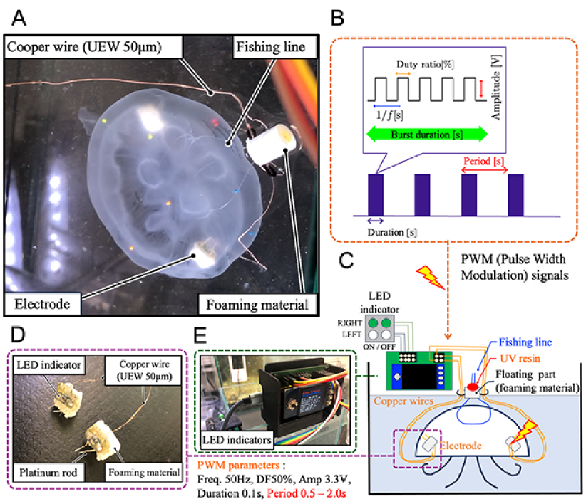
Figure 1: Overview of Electrostimulation Experiments: (A) Electrode-mounted jellyfish with the floating tethered system designed for this study. (B) Pulse width modulation (PWM) signals for jellyfish muscle stimulation that mimic neural commands to muscles. (C) Schematic of the proposed floating tethered system. (D) Electrodes with LED stimulus indicators and wires. (E) Custom-built electrical stimulator using a Raspberry Pi Pico W. Parameters of PWM signals are adjusted by a Python program implemented in the stimulator.

Jellyfish cyborg system for embedding embodied intelligence

To control a biological jellyfish cyborg that can utilize the interaction between its soft body and the water environment to generate efficient, adaptive, and flexible behaviors  (?, ?, ?, ?, ?), we developed a system that allows for quantitative and statistical data acquisition during stimulus intervention experiments while closely replicating natural floating behaviors (Fig. 1 A, supplementary video S1). Electrodes (Fig. 1 D) were inserted into the underside of the umbrellar body (Fig. 1 C) of the jellyfish (Aurelia aurita medusae, Fig. 2 A) to provide electrical stimuli to the coronary muscles  (?, ?, ?), which are located on the body. Pulse Width Modulation (PWM) signals (Fig. 1 B), which emulate neural commands to the muscles, were generated using a custom-developed electrostimulation device (Fig. 1 E) and applied to the electrodes to induce muscle contraction generating pulsatile motion. We systematically investigated the conditions that lead to effective floating locomotion in jellyfish by adjusting the parameters of the PWM signal (see Materials and Methods).

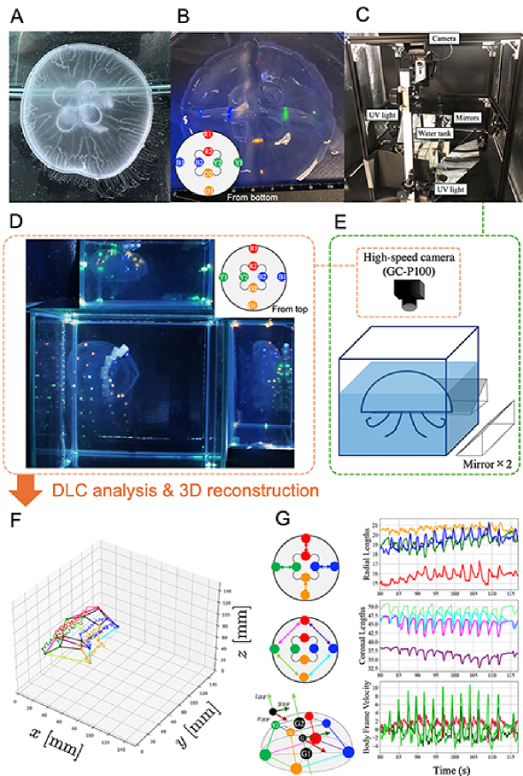
Figure 2: Experimental Animals and Setup: (A) Aurelia aurita medusae. (B) Visible Implant Elastomer Tag under UV light. (C) Measurement system with a high-speed camera. (D) Overlaid snapshots of camera images (every 6 seconds). Reconstruction and quantification of floating locomotion in a tank in three-dimensional (3D) space by estimating marker positions using DeepLabCut (DLC). (E) One camera from the top view and two mirrors on the sides of the tank for synchronized, simultaneous recording from three different directions. (F) Reconstructed 3D motion of spontaneous jellyfish floating. (G) Time-series data of radial and coronal lengths on the jellyfish body and 3D velocity in the defined BodyFrame.

To quantify the spatiotemporal response behavior of jellyfish to electro-stimulus and collect data for motion prediction using reservoir computing, we developed a custom 3D motion capture system, which allows us to measure jellyfish behaviors in a three-dimensional space within a water tank (see Fig. 2). The key features of our system include: (i) implementation of Visible Implant Elastomer (VIE) tag markers that reflect UV light (Fig. 2 B) to measure the deformation of the transparent jellyfish body, (ii) recording from three orientations using a top view camera and two mirrors (Fig. 2 C and E), and (iii) marker position estimation through DeepLabCut  (?) (Fig. 2 D) and 3D motion reconstruction (Fig. 2 F). With this system, we are able to quantify the jellyfish’s 3D floating trajectory in the tank (Fig. 2 F), collect time series data on the length between markers on the body, and measure the locomotion speed along the BodyFrame of the jellyfish (Fig. 2 G) (see Materials and Methods for more details).

Spontaneous pulsatile floating behavior

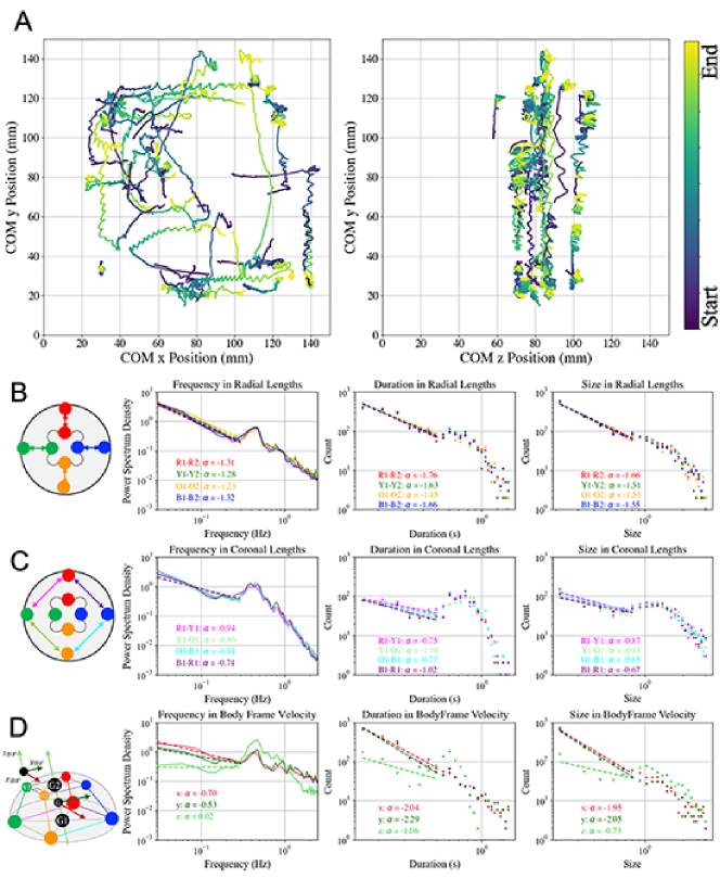
Figure 3: Spontaneous Pulsatile Floating Pattern: (A) 3D spontaneous floating trajectories in a water tank under analysis ($N=6$ animals, 37 trials). Left: top view ($x$-$y$ plane). Right: side view ($z$-$y$ plane). Color maps indicate the start and end of the measurement. (B), (C), and (E) Distribution of Power Spectrum Density (left column), Duration (center column), and Size (right column) for Radial length (B), Coronal length (C), and BodyFrame velocity (D). The vertical and horizontal axis scales are shown in the figure in log scale. The colors in the figure are R1-R2 (red), B1-B2 (blue), O1-O2 (orange), Y1-Y2 (green), R1-B1 (purple), B1-O1 (cyan), O1-Y1 (green), Y1-R1 (magenta), x velocity (crimson), y velocity (dark green), z velocity (lime green). Each dotted line in the figure represents a linear regression line in the corresponding region, and $\alpha$ is the value of the power exponent.

Fig.2 F illustrates the reconstructed 3D spontaneous pulsatile floating behaviors of the jellyfish in the water tank. The color trajectories (red, green, orange, blue) represent the VIE tags trajectories in the tank. The squares connected by lines demonstrate the deformation of the jellyfish body, connecting R1-Y1-O1-B1 (magenta, green, cyan, and purple colors) and R2-Y2-O2-B2 (all black colors) in the initial and final states. By comparing with the videos (supplementary video S2), we can confirm that the 3D motions can be qualitatively reproduced from the 2D video images.

Fig. 2 G displays the time evolution of the radial and coronal lengths calculated from the reconstructed marker positions. The line colors correspond to those of the jellyfish in the left panels of Fig. 2 G. We observed active oscillations for radial and coronal lengths generated through ring (subumbrellar) muscle expansion and contraction in the jellyfish body. The bottom panel in Fig. 2 G shows the velocity changes in the $x_{BF}$ (crimson), $y_{BF}$ (dark-green), and $z_{BF}$ (lime-green) directions in the BodyFrame defined for the jellyfish’s body. In the BodyFrame velocity, the increase and decrease of the velocity synchronized with the contraction of the body. The velocity changes in the $y_{BF}$ direction, which mainly corresponds to the direction in which the jellyfish was moving, and in the $z_{BF}$ direction, which corresponds to the direction above the bell of the jellyfish, are also notable.

Fig. 3 A displays the locomotion trajectories of spontaneous floating patterns in a 3D water tank ($N=6$ animals, $n=37$ trials). The trajectories are plotted in the $x$-$y$ and $z$-$y$ planes. The measurements were conducted over a relatively long time scale of 35–150 s, with the start and end times indicated by color scale (viridis). The initial position of the jellyfish was random. Notably, the height in the $z$-direction is constrained by the tethered floating system depicted in Fig. 1 C. We observed four types of spontaneous floating patterns: periodic pulsating straight locomotion, periodic pulsating rotational movements, a combination of these movements, and a resting state where the jellyfish remained stationary without pulsating. Some animals were unable to navigate around the walls or corners of the tank due to the limited range, and instead continued to pulsate.

To investigate the mechanisms inherent in the spontaneous floating pattern, we conducted a detailed analysis of the time series data for jellyfish body lengths including: radial lengths (B), coronal lengths (C), and BodyFrame velocity (D). In Fig. 3 B–D, the left column displays the frequency analysis (Power Spectrum Density) of these time series data on a logarithmic scale. Notable frequency peaks characterize the intrinsic pulsating motion with some variation occurring among individuals. A power law relationship is observed in linear regression lines up to the peaks: (B) $\alpha$ = 1.2 to 1.3; (C) $\alpha$ = 0.7 to 0.9; and (D) $\alpha$ = 0.5 to 0.7, except in the $z_{BF}$-direction, which has $\alpha$ = 0.02.

We extracted pulse-like oscillation waveforms from the time series data to evaluate the characteristics of Self-Organized Criticality (SOC)  (?, ?, ?). The presence of a power law in a phenomenon is an indication of the existence of SOC. We computed the duration (in seconds) and size (integral value, area) of the pulses, and their distribution is plotted in the center and right columns (see Materials and Methods for calculation details). The analysis results indicate that the radial lengths have durations and sizes of approximately $\alpha$: 1.4 to 1.7, the coronal lengths have $\alpha$: 0.7 to 1.10, and the BodyFrame velocity has $\alpha$: 2.0, except in the $z_{BF}$-direction.

Stimulated pulsatile floating behaviors

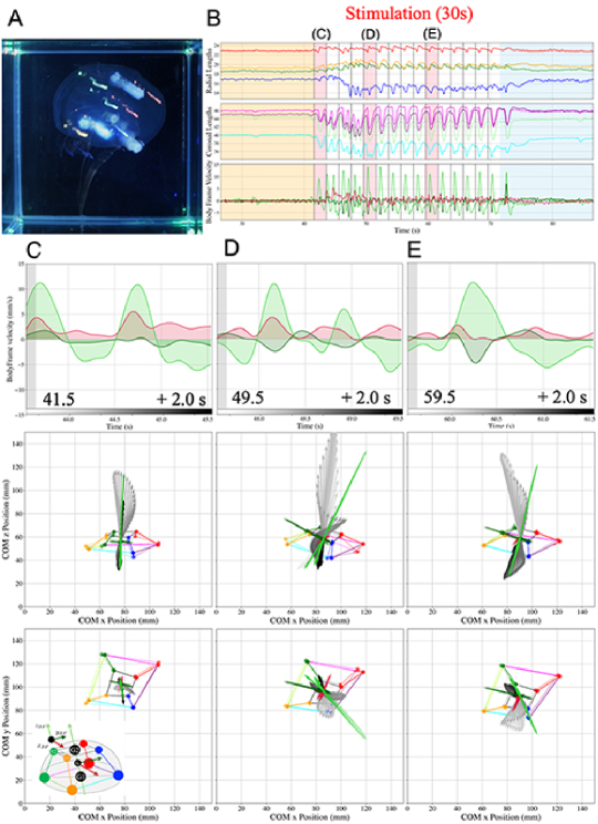
Figure 4: A representative example of the floating pattern induced by electrostimulation (supplementary video S3): (A) Locomotion trajectory of a jellyfish (top view) during the 30 s electrostimulation period. Overlaid snapshots are shown at 2.0 s intervals of the stimulation cycle (the closer to the stimulation start time, the higher the transparency). (B) Time series data of radial and coronal lengths, and BodyFrame velocities including periods before, during, and after electrostimulation (yellow: before 15 s, white: stimulation 30 s, sky-blue: after 15 s). The pink highlights indicate one cycle (2.0 s) of electrostimulation in (C)-(E) below. (C), (D), (E) Top row: Velocity changes in $x$ (crimson), $y$ (dark green), and $z$ (lime green) directions in the BodyFrame during the corresponding one stimulus cycle (2.0 s). Middle row: Jellyfish position at the beginning and end of stimulation, and the time evolution of the velocity vector during electrostimulation in the $x$-$z$ plane (side view) of the tank. Velocity vectors change in shade of black from the beginning to the end of the 2.0 s stimulation. The velocity vectors in the $x$-, $y$-, and $z$-axis of the BodyFrame are also shown in each color. Bottom row: Identical data as in the middle row, displayed in the $x$-$y$ plane (top view).

Fig. 4 illustrates the floating pattern observed when a 2.0-second periodic electrical stimulus was applied to the electrode between O1-B1. The following parameters of the PWM signal were kept constant in the experiments: frequency (f) is 50 Hz and duty ratio is 50%. Preliminary (trial and error) experiments determined these parameters effectively generated pulsatile motion. Here, we investigated how the pulsatile motion varied by adjusting the stimulation period (Fig. 1 B). To analyze changes in behavior before and after electrical stimulation, we quantified the floating patterns during three time intervals: 40 seconds before, 30 seconds during, and 40 seconds after the periodic electrical stimulation. As a control condition, we also conducted experiments without stimulation for 150s intervals using the floating tethered system and electrodes, referred to as the "w/o stimulation" condition.

Fig. 4 A shows the superimposed top view of the camera that measured the locomotion trajectory of the jellyfish during 30 seconds of electrical stimulation, with intervals of $2.0s$ of the stimulation cycle. In Fig. 4 B, the time series data of radial lengths (top), coronal lengths (middle), and BodyFrame velocity (bottom) are shown for $15s$ before (yellow) and $15s$ after stimulation (light blue). We observed a pulsatile pattern during the electrostimulation period, characterized by contraction and increased velocity, mainly in the $y_{BF}$- and $z_{BF}$-directions, which synchronized with the input period. Fig. 4 C–E depict the changes in BodyFrame velocity (top), the position of the jellyfish before and after stimulation (center and bottom), and the projection of the BodyFrame velocity vector trajectory onto the $x$-$z$ plane (center) and transverse plane (bottom) during the relevant period of the electrostimulation in Fig. 4 B (highlighted in pink). The figure illustrates that the velocity change in the $z_{BF}$ direction was mainly induced in the initial stimulus period, while the velocity vector in the $x$-$y$ plane was induced in the latter half of the stimulus period. Specifically, during the 2.0 s of the stimulus cycle (especially in E, which settled into a steady pattern), in the first half of the stimulus period just after $0.1s$ of electrostimulation (start to around $1.0s$, gray arrows), velocity vectors in the direction of travel in the $x$-$y$ plane and the positive direction of $z_{BF}$ were induced. In the second half (from around $1.0s$ to the end, black arrows), on the other hand, the velocity vectors in the opposite direction to the locomotion direction in the transverse plane and in the negative direction of $z_{BF}$ were induced. These changes in the velocity vectors contribute to the increase or decrease in the whole-body velocity of the jellyfish during one stimulus cycle, resulting in muscle stimulus-induced locomotion.

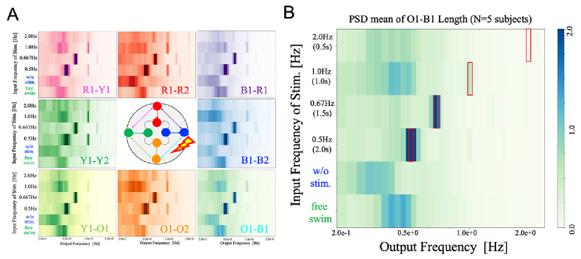
Figure 5: Spatiotemporal pulsatile floating pattern analysis for electrostimulation: $N=5$ subjects. Comparison in four stimulus input conditions: 2.0 s, 1.5 s, 1.0 s, 0.5 s. We conducted 5 trials for each condition, randomizing the order of conditions. We fixed the wires between R1 and Y1 and between O1 and B1, applying a PWM signal only to the electrode between O1 and B1. (A) Frequency response (Power Spectrum Density: PSD distribution) for each spatially distributed radial and coronal length. (B) Detailed display of frequency analysis (O1-B1) for four stimulation input conditions, no electrostimulation with wires (w/o stim column), and spontaneous floating motion (free swim column). Vertical and horizontal axes indicate input and output frequencies, respectively, and color shading indicates PSD. The red squares were displayed in the areas corresponding to the input frequencies for the four conditions.

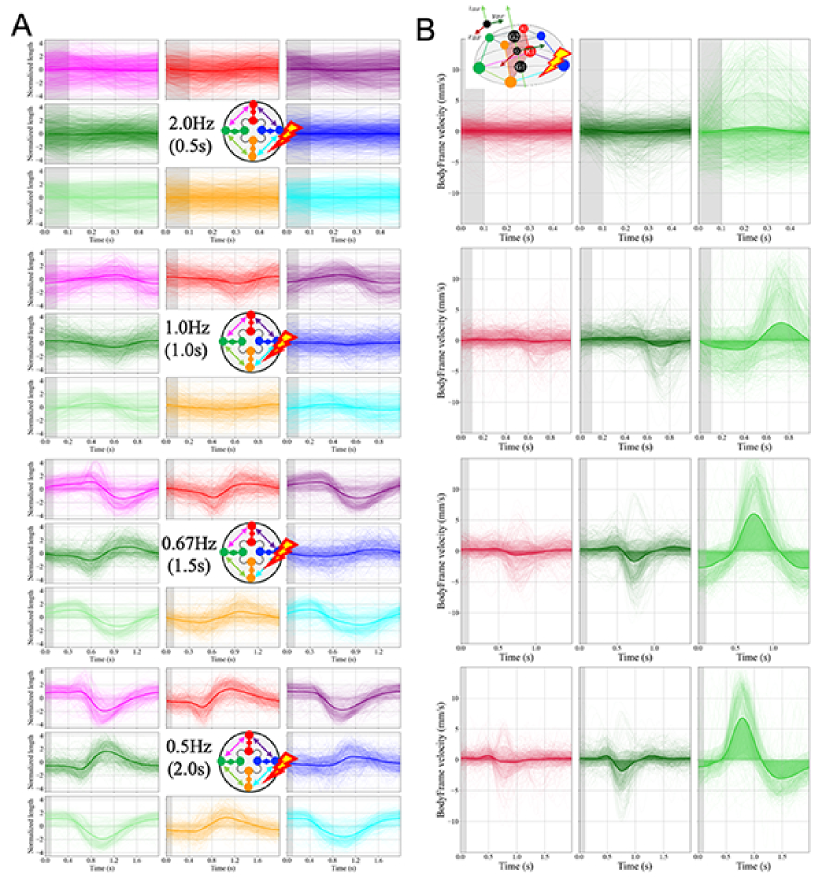
Figure 6: Phase response for electrostimulation: (A) Phase response analysis for radial and coronal length (normalized length data) for each condition (0.5 s, 1.0 s, 1.5 s, 2.0 s from the top). Each time series data set was segmented and overlaid at each input stimulus period ($N=5$ subjects, 5 trials per condition). The dark line indicates the mean trajectory. (B) Phase response analysis of $x$ (crimson), $y$ (dark-green), and $z$ (lime-green) velocities on the BodyFrame for each condition (0.5 s, 1.0 s, 1.5 s, and 2.0 s from the top) (data extraction and display methods are similar to (C)). The average velocity is indicated by a bold line, and the region between the average velocity and velocity 0 is indicated by the corresponding transparent color.

Fig. 5 A shows the frequency response of the radial and coronal lengths in the jellyfish body ($N=5$ animals) when subjected to electrical stimulus input on the ring muscle. The input is provided from an electrode positioned between O1 and B1. The color map corresponds to the lengths associated with each color. Fig. 5 B provides a closer look at the frequency response for the lengths O1–B1, offering a more detailed interpretation of Fig. 5 A. The vertical axis of Fig. 5 B represents the frequency of the electrical stimulation input. The resulting frequency responses, corresponding to stimulation inputs of $0.5s$, $1.0s$, $1.5s$, and $2.0s$ periods (4 conditions) from the top, are displayed on the horizontal axis. The Power Spectrum Density (PSD) values are represented by the color shade. The “w/o stimulation” column presents the frequency response in the presence of wires but without electrostimulation, while the “free swim” column represents the frequency response during spontaneous floating as demonstrated in Fig. 3. The red square in Fig. 5 B indicates the input frequency. Fig. 5 A reveals that there is no significant difference between the spatial location of the input stimulus (O1–B1) and the frequency response of each body part.

Fig. 6 A illustrates the phase response of body length (radial and coronal lengths) to periodic electrostimulation inputs. The periods include $0.5s$, $1.0s$, $1.5s$, and $2.0s$. The pulses of each input frequency are depicted showing the normalized length time variation during the 30 s electrostimulation period. The gray shaded regions represent the $0.1s$ period when the PWM signals were injected. The color of each plot corresponds to the length color located on the jellyfish body. Bold lines indicate the average change in length for $N=5$ subjects with 5 trials per condition. Notably, we observed coherent length changes in the $1.5s$ and $2.0s$ input conditions, coinciding with the frequency peaks depicted in Fig. 5 A. Contraction and expansion changes in length were clearly observed in these input conditions, suggesting the generation of pulsatile motion synchronized with the input frequency. In contrast to the frequency response, a spatial distribution of the phase response was observed, characterized by a phase-time response curve symmetrical to the line between the jellyfish body center of mass and the electric stimulus point (midpoint of O1 and B1): thus, the response curves for B1-B2 (blue) and O1-O2 (orange), Y1-O1 (light-green) and B1-R1 (purple), and Y1-Y2 (green) and R1-R2 (red) were identical, respectively. This indicates the generation of a contraction/relaxation progression in the jellyfish body from the stimulation point. Furthermore, the response curves for the $1.5s$ and $2.0s$ input conditions confirm that the period characterizing contraction/relaxation for each length is approximately $1.6s$.

Fig. 6 B displays the phase response of BodyFrame velocity to electrostimulation frequency inputs ($0.5s$, $1.0s$, $1.5s$, and $2.0s$ periods). The plotting method is the same as in Fig. 6 A. Bold lines represent the change in the mean value for $N=5$ subjects with 5 trials per condition. To clarify positive and negative changes in velocity, the same transparent color is used between the mean velocity and velocity 0. Similar to the findings in Fig. 6 A, coherent changes in BodyFrame velocity were observed in the $1.5s$ and $2.0s$ electrostimulation input conditions. Notably, the velocity in the $z_{BF}$ direction was positive in the first half of the stimulus input (around $1.0s$ from the start) and negative in the second half (around $1.0s$ to the end). Conversely, the velocity in the $y_{BF}$ direction was negative in the first half and positive in the second half, albeit not as clearly as $z_{BF}$. In the $1.5s$ and $2.0s$ conditions with distinct frequency responses, the progressive waves of contraction/relaxation in the jellyfish’s soft body that induced by the muscle electrostimulation, resulted in velocity change in the BodyFrame. This change would contribute to the locomotion direction of the floating jellyfish.

Verification of stimulus location and locomotion direction

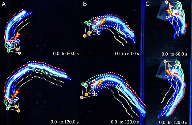
Figure 7: Direction control experiments were conducted using 2.0-s period electrostimulation, which effectively induced pulsatile locomotion. These experiments lasted for 120 seconds and aimed to determine the relationship between the stimulus input position and the direction of locomotion. The jellyfish locomotion was observed in a water tank with inserted UV reflective markers (VIEs), solely from a top view. For the electrostimulation, only one wire was inserted at the midpoint between R1 and B1. To visualize and plot the trajectories, movies were superimposed at 2.0s intervals. In figures (A), (B), and (C), the trajectories starting from different initial positions and postures (orientations) in the tank are depicted. The upper row displays the trajectory between 0 and 60 s, while the lower row shows the trajectory between 0 and 120 s.

To demonstrate the possibility of controlling the direction of jellyfish locomotion through muscle electrostimulation, we conducted experiments to investigate the relationship between the position of the stimulus input and the direction of locomotion. Using only one electrode, we performed continuous electro-muscle stimulation experiments for 120 seconds. Figure 7 illustrates the locomotion trajectories of jellyfish starting from different initial positions and postures (orientations) in the tank. The upper row shows the trajectory from 0 to 60 seconds, while the lower row shows the trajectory from 0 to 120 seconds. We inserted UV reflective markers (VIEs) into the jellyfish and recorded only the top view. The results in Figure 7 (supplementary video S4) demonstrate that the jellyfish tended to move in the direction of the midpoint between R1 and B1, where the electrostimulation was applied to the muscles, regardless of the initial position and posture of the jellyfish. The curved trajectory during electrostimulation suggests that the wire tension affected the trajectory.

Motion Prediction with Reservoir Computing

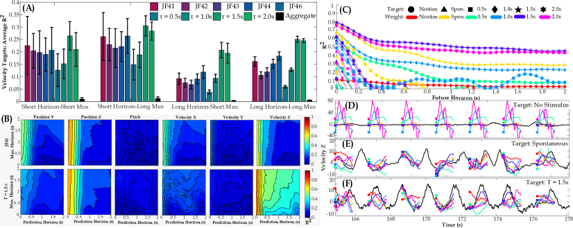
Figure 8: Results of Jellyfish motion prediction RC. A) Average and standard deviation of $R^{2}$ for several training schemes organized by both specimen (indicated by JF and a number) and stimulus. B) Shows the $R^{2}$ values for 6 of the different targeted whole body motions for both a test organized by specimen and organized by input stimuli. C) Shows $R^{2}$ for a confusion task with weights trained on different types of organized pulse being used to emulate vertical velocity targets of both trained and untrained data. A set of 1 second velocity predictions using different training weights emulating vertical velocities during: D) free swimming motion with some spontaneous pulses, E) collected spontaneous pulses, and F) pulses stimulated at $1.5s$ intervals. The black line shows the target response while the predictions are depicted following the colors from C.

Fig.8 shows the results of a "Hybrid" reservoir computer configuration that fuses an echo-state network (ESN)  (?) and a PRC to predict future motions of the Jellyfish including relative position, angular rotations, and BodyFrame velocities (see Materials and Methods for RC settings). The jellyfish states injected to the RC (i.e. ESN inputs and outputs of the PRC) come directly from a "Best" sensor configuration made up of the lengths: outer radius, inner radius, Y2–O1, and R2–O2 (see Supplementary Material S5 and S8 for how the sensor and hybrid configuration were selected).

To compare the performance using different training data, the Hybrid RC was trained on stimulated pulsatile data aggregated and grouped by animal specimen and stimulus period. Fig.8A shows the four quadrant averaged $R^{2}$ values for all velocity targets for each on different data groupings.The four quadrants of estimated data are averaged on “Short” horizons, including data from $(0s,1s]$ in the future, and “Long” horizons including data from $(1s,2s]$ in the future, for the input multiplexing (mux) and predictions. $R^{2}$ trained on all Jellyfish aggregated data is also depicted for comparison. Training the data on only the bodies motions during stimulated intervals significantly improves the velocity predictions while the aggregated data performing only marginally better than a regression fit. The highest reconstruction accuracy occurs in data organized and trained on the input stimuli $\tau=1.5s$ and $\tau=2s$. These periods also correspond to the COM and relative marker position profiles with the most consistency across different tests and specimen. These stimuli also have particularly good accuracy for long horizon predictions with higher average values than even RCs trained on $\tau=0.5s$ and $\tau=1s$ over short prediction horizons. RC’s trained on individual specimen also show good performance in short horizon cases with JF41 and JF46 showing comparable performance to $\tau=2s$ trained RC.

Further illustrating the differences between training type, Fig.8B shows value of $R^{2}$ of the RC for 6 of the targets (2 periodic positions, the best captured body rotation, and the 3 BodyFrame velocities) trained on stimulated data for combined tests on specimen JF41 and at $\tau=1.5s$. The vertical (Z direction) motions of the Jellyfish are captured the best in the RC framework. Peak $R^{2}$ values for vertical position are $0.81$ and $0.74$ and for vertical velocity $0.68$ and $0.79$ for JF41 and $\tau=1.5s$ cases respectively. The body rotations, such as the shown pitch angle, are poorly approximated. Body rotations during testing generally slow and of a small magnitude across individual pulses. Further, we did not find a strong indication of these motions synchronizing with the current stimulus method. For JF41, transverse plane (x-y) velocity predictions exceed $R^{2}$ values of $0.5$ while the $\tau=1.5s$ case has all other velocity predictions below $0.3$. It was noted that individual specimen often had similar net velocity directions during stimulus but only the vertical directions appeared consistent across specimen, likely causing this feature. While the input organized RCs shows much better predictions of the vertical motions for long horizons (in the longest multiplex case the z velocity $R^{2}$ value falling below $0.5$ after $1s$ ), the specimen organized RC show better all around short predictions for very short horizons.

To analyze estimation of untrained regions and the information encoded in the RC, weights were trained on the free swimming data (both in aggregate and limited only to the spontaneously occurring pulses) and on each of the input stimulus periods’ pulsatile responses. Fig.8 C shows the confusion $R^{2}$ results for predicting future vertical velocities with each trained weight set emulating each training target. Each of these predictions used the $2s$ mux input data for the RC. Fig.8 C does not depict any $R^{2}<0$. While each weight matrix best predicts the velocity on which is was trained for both, a few weights can also achieve high prediction accuracy’s in short horizons for untrained targets. Most notably the data trained on spontaneous pulses, $\tau=1.5s$, and $\tau=2s$ all achieve have $R^{2}>0.4$ when emulating one another. Additionally, $\tau=1.0s$ was also able to emulate the stimulated behavior for $\tau=1.5s$ and $\tau=2s$. Contrarily, the free swimming behavior both poorly predicts other targets and is poorly predicted by any training data set. Only its own trained weight set can predict the free swimming data with a positive $R^{2}$.

To illustrate this, $1s$ predictions are shown emulating free swimming with some spontaneously occurring pulses in Fig.8 D. The $\tau=1.0s$ and $\tau=2.0s$ intervals significantly over-predict the motion of the free swimming behavior. The spontaneous and $\tau=1.5s$ weight set exhibit similar magnitudes to the spontaneously occurring pulses response but poorly predict waveform shape when the body is at rest. In contrast, predictions of only spontaneous pulses (Fig.8 E) are matched well in both direction and magnitude for short horizons with all stimulus period weights during a pulse. Estimates are particularly good when the velocity is decreasing, likely owing to the body having a similar relaxation motions after muscle contraction. The worst estimates occur when there are longer or inconsistent intervals between pulses. This facet is largely remedied during stimulation (Fig.8 F) that enforces a regular interval. Notably the self trained weights in Fig.8 F follow the pulse shape closely over each of the depicted $1s$ horizons.

These results show that whole body motions can be emulated with high accuracy using data from the Jellyfish’s body. While difficult to predict the occurrence of spontaneous pulses, the body can be used to predict motion well during input stimulus, and better when the inputs stimuli synchronize with the bodies natural pulsate swimming.

Applicable RC

A viable version of the Hybrid RC was composed that could be run on a commercially available 3.5 $cm^{2}$ microcontroller: the SEEED Xiao SAMD21 (shown in Fig. S9). Testing of RC forms and processing speeds it was found that the largest form of the hybrid RC that could efficiently compute the targets and be run in real-time (set by the camera frame rate) was a 35 node ESN input with instantaneous sensor data with only the PRC receiving temporal multiplexing (see supplementary materials S10). In addition the output state also included 3-axis IMU acceleration data, as this was determined to improve the accuracy while being among the easiest small scale sensors to include on the animal without directly interfering with body motion. The projected $2s$ predictions for six instances over a $2s$ pulse are shown in Fig. 1S. This RC was trained on the $\tau=2.0s$ data set targeting velocity with the position predictions for the local movement estimated via dead-reckoning (to see results from additional trained tests see supplementary video S7).

As in earlier results the velocity predictions of the motions in z are the best and accurately capture both the magnitude and shape very well. In this direction $R^{2}$ value for velocity was 0.7306 for estimates of the current position and 0.39 for the final position holds a value above 0.6 for the first 10 time-steps. Both x and y velocity predictions match the general behavioral shape with attenuated magnitudes, most notably so in y. The velocity $R^{2}$ values ranged between 0.21 and 0.165 (at $t=+1.6s$) in x and 0.148 and 0.07 (at $t=+2s$) in y. The positional predictions also match the shape of the position trajectory. The average errors in the prediction tails ($t=+2s$) where the position predictions deviate the most are x:0.007, y:0.0032, and z:0.0087. In 3D these appear to follow the sample motion profile with an attenuated magnitude largely in the y direction. The best predictions for all motions generally occur after the body has fully contracted ($t>0.8s$) while the worst occur immediately prior to the next pulse where the body is near its natural rest state. While the predictions shown here may not all be useful as far $2s$, shorter horizons do show good predictability.

Discussion

The goal of this study is to develop a control system for a jellyfish cyborg robot that effectively harnesses the self-organized adaptive abilities, known as “embodied intelligence,” which are naturally embedded in biological animals. The model animal, jellyfish (Aurelia aurita medusa), is chosen because it is among the most energetically efficient aquatic animals  (?, ?), despite its simple neural structure and lack of a brain  (?, ?, ?, ?). This efficiency is achieved by effectively utilizing the interaction between its soft body deformation and the hydrodynamics of the environment  (?, ?), which we refer to as “embodiment  (?).” In order to study this phenomenon, we have developed a tethered floating system that intervenes in jellyfishes’ floating locomotion by applying electrostimulation to the coronal muscles of its body. We have also constructed a custom-built measurement system to quantify and analyze jellyfishes’ three-dimensional locomotion in the aquatic environment. Additionally, we have applied an extended framework of reservoir computing (?, ?) to predict jellyfish locomotion using the accumulated data from both spontaneous and electrostimulation-induced locomotion. This study is the first to successfully incorporate the dynamical motion data generated from the interaction between an animal’s body and its environment into an “embodied” reservoir computing framework to predict animal locomotion.

Using our developed measurement system, we estimated the position of VIE tags injected into the transparent body of jellyfish, allowing us to quantify the spatiotemporal deformation patterns of floating jellyfish that exhibit spontaneous pulsation. Our analysis confirmed the characteristic contraction-relaxation of the jellyfish’s soft body shape during spontaneous floating, as well as the associated locomotion velocity along the defined BodyFrame, and the time-series data of the macroscopic locomotion trajectory in the 3D aquarium (Fig. 3). Frequency analysis of the time-series data revealed two essential findings. Firstly, there was a frequency peak (around 0.45 Hz) corresponding to the spontaneous period of jellyfish locomotion. Secondly, there was a power law observed in the frequency region up to the peak, except for the $z_{BF}$ velocity. It is worth noting that the body size of the jellyfish used in this study ranged from 55 to 80 mm, and there was no significant variation in body size, explaining the lack of individual differences in the intrinsic frequency peak of locomotion. The absence of a power law for the $z_{BF}$ velocity, unlike other variables, can be attributed to the weak motion constraint in the $z_{BF}$ direction imposed by the adopted tethered floating system. To further investigate the SOC characteristics  (?, ?) in jellyfish locomotion, we extracted pulse-like patterns from the time-series data and quantified the duration of one pulse cycle, as well as its size (integral value and area) (see Fig. LABEL:fig:duration_size). As illustrated in Fig. 3 B-D, the fact that a power law was also observed for the duration and size of the pulses suggests the presence of SOC in the spontaneous floating motion of jellyfish. Previous studies  (?, ?) have examined the frequency response of jellyfish muscles to electrostimulation while placed on a dish, but our study is the first to reveal the frequency response during spontaneous locomotion. Additionally, there have been no prior investigations into the characteristics of SOC in the spontaneous locomotion of jellyfish.

The muscle electrostimulation experiment confirmed that changing the period of input rectangular pulse using the PWM signal (Fig. 1 B) altered the pulsatile frequency and BodyFrame velocity (Figs. 5 and 6). To the best of our knowledge, this is the first frequency and phase response analysis of jellyfish floating locomotion induced by muscle electrostimulation, rather than jellyfish placed on a dish  (?, ?). The phase response analysis for controllable frequencies (Fig. 6 A, specifically 1.5 s and 2.0 s) provides three notable suggestions: (i) From the 2.0 s period experiment, the characteristic period of contraction/relaxation of jellyfish muscle induced by electrostimulation input is approximately 1.6 s, and the time constraint of this muscle contraction was the basis for the reduced responsiveness of the 0.5 s and 1.0 s stimulus input. (ii) The phase response curves of the 1.5 s and 2.0 s input periods are symmetrical with respect to the line connecting the center of the jellyfish body and the electrostimulation position, i.e., O1-O2 and B1-B2, O1-Y1 and B1-R1, and Y1-Y2 and R1 and R2 are comparable. This indicates that the muscle contraction/relaxation within the jellyfish’s soft body propagates spatially from the location of the electrostimulation toward the body center. (iii) Coherent and consistent phase responses to the 1.5 s and 2.0 s inputs, where peaks in frequency response are observed, suggest that the responses to these input parameters possess an Echo State Property (ESP)  (?), which is a condition that can be used for reservoir computing of the jellyfish’s floating motion. The velocities along the BodyFrame induced by electrostimulation (1.5 s and 2.0 s period) exhibit the largest positive peak in $z_{BF}$ and a small negative peak in $y_{BF}$ during one cycle of electrostimulation, but no significant peak in the $x_{BF}$ direction (Fig. 6 B). This lack of a peak was due to the large deviations in $x_{BF}$ and $y_{BF}$ velocity for each individual. These deviations are caused by the influence of the electrode weight on the jellyfish body shape (difficult to perfectly balance the weight to 0 g underwater) and the inability to achieve completely uniform and symmetric conditions, such as the inserted electrode position. Nevertheless, the case of one jellyfish shown in Fig. 4 and the results of the directional control experiment indicate that the locomotion direction in the macroscopic $x$-$y$ plane tends to move from the jellyfish body center toward the electrostimulation point, suggesting the feasibility of directional control for a jellyfish cyborg. The changing profile of the $x_{BF}$ and $y_{BF}$ velocity vectors (Fig. 4 C and D), due to the spatial pulsatile propagation of the jellyfish’s soft body deformation induced by the electrostimulation described above, adjust the jellyfish’s “posture” and changes the direction of the “dominant” $z_{BF}$ velocity vector, resulting in locomotion toward the stimulus position.

We have shown the current state of a jellyfish’s body provides information that can be used to directly estimate its current whole body motion and, indeed, future motions. Incorporating an ESN and/or a number of past states of the body can significantly improve these estimations. Estimates with aggregated data show the jellyfish’s body provides little information to “telegraph” when a pulse will occur or if these pulses will exhibit a maneuver other than a vertical motion. Spontaneous pulses occur due to neural signals possibly induced by environmental stimuli but generally appear to be random or exploratory motions that are difficult to predict. However, the motion of the pulses themselves can be predicted fairly well from visible morphological states. Thus when stimulus is injected that can consistently induce pulsing motions, the animals’ swimming becomes predictable. Furthermore, stimuli that synchronize with the jellyfish’s natural pulsing dynamics (such as periods $\tau=1.5s$ and $\tau=2.0s$) result in better predictions and faster swimming. These pulses have the added benefit of functioning as a good data source to predict the motions of the natural swimming pulses (at least for short horizons $<0.2s$). Although predictions of vertical motions are good, from the data collected here it is difficult to estimate rotational motion and estimates are fair to poor of motions directed in the transverse plane. While tests across specimen did not always result in the same direction of motion in the transverse plane during stimulus, individual specimen often did have consistent motions in these directions when stimulated (likely owing to variability between animals and the placement of the electrode). As a result, estimation of individual animals improved in the transverse plane. This suggests that, in future, other directions and rotations can likely be predicted provided a stimulus method that can consistently induce these motions across specimen. As it was demonstrated that these predictive models can be computed directly on a small microcontroller, integrating them with an established autonomous control system is a simple task. With both prediction and control functionality, higher level control architectures such as model predictive control may be implemented directly on a small scale jellyfish cyborg while preserving its embodied intelligence.

Still, there are several limitations to the experiments in the present study. First, it is not possible to completely eliminate the effects of physical properties such as electrode weight and wire tension needed for electrostimulation in an underwater environment. One possible solution is to use larger individual jellyfish, specifically those larger than 200 mm, where the impact of electrodes and wires is less significant. Another option is to transform the system into a fully mobile cyborg robot, as seen in previous studies  (?, ?). Second, we have not yet validated the simultaneous or time-delayed electrical stimulation input using multiple electrodes. Initially, our study involved four electrodes attached to the jellyfish body. However, the weight and tension of the electrodes and wires proved to be a significant issue as described above, twice as large compared to using two electrodes. By addressing this problem and implementing electrical stimulation at multiple locations, we can anticipate the possibility of generating complex locomotion trajectories by integrating the findings from this study on one-electrode electrostimulation. Third, our study used a relatively small water tank (150mm$\times$150mm$\times$ 150mm) due to the limitations of the measurement environment. As a result, we faced restrictions on the duration of spontaneous floating locomotion without external environmental input. Furthermore, after stimulation, we observed in some trials that locomotion near the tank wall was almost immobile due to physical constraints. Expanding the measurement system to larger tanks in the future will enable us to gain a better understanding of the characteristics of long-duration and long-distance locomotion. On the other hand, to ensure more systematic data acquisition, we designed a measurement system specialized for the laboratory environment. The primary goal was to accumulate data for a comprehensive understanding of the locomotion principle and its application to physical reservoir computing. The precise data obtained from this measurement system, along with knowledge of frequency response, phase response, velocity characteristics in BodyFrame, and motion prediction using embodied reservoirs, will contribute to the development of a jellyfish cyborg control strategy that maximizes its potential abilities, such as efficiency and adaptability derived from its embodiment. To successfully develop jellyfish cyborgs that aid in ocean exploration and marine pollution abatement, it is crucial to enable behavioral control according to the desired objective while preserving the jellyfish’s embodied intelligence.

Materials and Methods

Animals

Aurelia aurita medusae were obtained from Kamo Aquarium (Tsuruoka, Yamagata Prefecture, Japan). The specimens were kept in specially designed aquariums for jellyfish (Kuranetarium, Nettaien, Miyagi Prefecture, Japan) and maintained at a temperature of 21$\sim$25^∘C. The aquariums were filled with natural deep seawater pumped from the ocean at a depth of 800 meters (Najim 800, bluelab, Shizuoka Prefecture, Japan), which helps to maintain jellyfish in a healthy state for longer. We collected data from six animals ($N=6$) in spontaneous floating experiments, and five of these animals were used in electrical stimulation experiments ($N=5$). Two additional jellyfish were used for the directional control experiments.

Ethics

Currently, jellyfish research at Tohoku University and the University of Tokyo is not subject to animal care regulations. We strongly support the ethical considerations and responsibilities discussed by  (?) with regard to animal experiments, whether they involve invertebrates that do not require specific approval or vertebrates that do. In our jellyfish experiments, we followed the principles of harm minimization, precaution, and the 4Rs (reduction, replacement, refinement, and reproduction). Furthermore, we fully agree with the authors that future research on cyborgs, which may explore ethical boundaries not yet fully considered by ethicists and legislators, will require careful consideration of both animal welfare and social consequences  (?).

Experimental setup

We constructed a system to measure and quantify the spatiotemporal patterns of three-dimensional (3D) floating movements in a glass water tank (150mm $\times$ 150mm $\times$ 150mm) (Fig. 2 C). The goal was to capture the jellyfish’s spontaneous pulsatile floating motion while adhering to measurement constraints. To efficiently analyze the 3D motion, we designed a measurement system that utilized a single camera positioned above the tank and two mirrors on the tank’s sides. This setup allowed for synchronized, simultaneous recording from three different angles (Fig. 2 E). The high-speed camera (GC-P100, JVCKENWOOD Corporation) was used to record the jellyfish’s motion data (videos), which were stored on an SD memory card in the camera.

The jellyfish’s body is mostly transparent, making it difficult to analyze the spatiotemporal patterns of its pulsatile floating motion from videos taken in its natural state. To address this, we used biocompatible Visible Implant Elastomer (VIE) Tags  (?), which are reflective markers visible under UV light. We injected VIE tags in four different colors at eight different locations on the jellyfish’s body, as shown in Fig. 2 B. These tags served as position markers for subsequent video analysis.

Electrical stimulation

We developed a custom-built electrical stimulator for stimulating jellyfish muscles (Fig. 1 E). An extension circuit board was designed for Raspberry Pi Pico W (Raspberry Pi Foundation), which included 4-channel Pulse Width Modulation (PWM) signal outputs. The parameters of the PWM signals, such as frequency $f$ (50 to 150 Hz) and duty ratio (0 to 100%), were changed using a Raspberry Pi microprocessor. This allowed us to investigate the effects of these parameters on motion generation due to muscle stimulation. Here, the frequency $f$ was set to 50 Hz, duty ratio was set to 50%, amplitude was 3.3 V, and duration was set to 0.1 s. We systematically analyzed behaviors generated by muscle contraction induced by bursts of PWM pulses. To do this, we varied the period [s] of the PWM signal and identified the condition that most effectively and repeatably produced pulsating motion.

The two wire electrodes were composed of copper wires with a diameter of 50 $\mu$m, platinum rod tips with a diameter of 254.0 mm (A-M Systems, Sequim, WA, USA), and tiny chip-LEDs (TinyLily 10402, TinyCircuits, Akron, OH, USA) as indicators of electrical simulations (Fig. 1 D). The electrode weight was offset with foam material to keep it approximately neutrally buoyant. A pair of stimulation electrodes were bilaterally implanted into the subumbrellar tissue of jellyfish near the bell margin (Fig. 1 A and C).

In stimulated floating experiments where electrodes with copper wires are used, it is mechanically impossible to completely eliminate the influence of wire forces. However, we made efforts to minimize the effect of the wires on jellyfish motion. To achieve this, we developed a floating tethered system that would maintain the jellyfish umbrella in a reasonably constant orientation while keeping wire tension as low as possible, as shown in Fig. 1 A and C. In this method, we threaded a fishing line (blue line in Fig. 1 C) through the gelatin (water) part of the jellyfish’s body, which does not affect its movement. We then fixed the endpoints of the fishing line to the foam material with UV resin (red ellipsoid in Fig. 1 C). This tethered method allowed the jellyfish to maintain the umbrella orientation within a range where it would not flip upside down, while still exhibiting its spontaneous floating behaviors. Fig. 1 A shows a photograph of a jellyfish specimen where the tether system was successfully implemented to produce a natural pulsating floating motion with wires and electrodes for stimulation.

Data Analysis

To quantify the pulsatile floating patterns in 3D space based on the 2D high-speed camera images (1920 $\times$ 1080 pixels at 60 fps), we used a pose estimation algorithm called DeepLabCut (DLC)  (?, ?). First, we marked training data (50-200 frames for each condition, such as spontaneous floating) to train the algorithm. This allowed the algorithm to automatically estimate 12 positions, including the four corners of the tank and 2 $\times$ 4 color markers on the jellyfish (as shown in Fig. 2 B), in three camera views (top:c, and from behind:u and from right:r in the mirrors). This resulted in a total of 36 positions (c1, c2, c3, c4, cR1, cR2, cY1, cY2, cO1, cO2, cB1, cB2, u1, u2, u3, u4, uR1, uR2, uY1, uY2, uO1, uO2, uB1, uB2, r1, r2, r3, r4, rR1, rR2, rY1, rY2, rO1, rO2, rB1, and rB2) during each trial of the experiment (Fig. S11). The pose estimation error after processing with DeepLabCut was less than 2.0 pixels (1920 $\times$ 1080 video pixels), indicating that the estimation accuracy was sufficient for further analysis.

The marker estimation using DLC provided 2D positions from three different directions. It’s important to note that the data obtained from these directions are temporally synchronized because they were captured by a single camera. While there are methods available to reconstruct 3D positions from 2D image data, for simplicity of analysis, we approximated the 3D positions using the estimated 2D positions in the $x$, $y$, and $z$ directions. However, since the four corner landmarks of the water tank do not form a perfect rectangle, we applied a homographic transformation to obtain compensated 2D positions, ensuring that the landmark appeared as an exact rectangle on the water tank.

Using the reconstructed 3D positions of the eight VIE Tags injected into the jellyfish body (R1, R2, Y1, Y2, O1, O2, B1, and B2, Fig. 2 F), we analyzed the pulsatile floating patterns in the water tank. All lengths between markers were calculated. In particular, we focused on the radial lengths (the four lengths between R1 and R2, Y1 and Y2, O1 and O2) and the coronal lengths (the four lengths between R1 and Y1, Y1 and O1, O1 and B1, B1 and R1) to quantify the spatiotemporal floating patterns (Fig. 2 G left). For analysis and RC training, relative body motions were extracted from the marker position data (Fig. 2 G bottom). The outer markers (index 1) and inner marker (index 2) were grouped as separate planes (G1 and G2 respectively) of the jellyfish with the global center of mass (COM) selected to be the center of the inner markers as these are closer to the thicker center of the bell. The average distances from the COM and the inner and outer maker sets was computed and denoted as the inner and outer radii. Euler (Z-Y-Z) rotations were used to set the animals’ body data into an identical local BodyFrame (denoted by BF in Fig. 2 G bottom). The first two rotations set the line segment between the centers of outer and inner planes of markers to be exactly along the vertical Z direction, and the final rotation was selected such that the line segment Y2-O2 to was fixed to the x-z plane.

During the stimulation experiments, we used four LED indicators to synchronize the stimulus input signals with the analyzed video images. The pair of LEDs indicated the left (white LEDs) and right (green LEDs) electrodes, with one LED indicating “ON” and the other indicating “OFF” for the simulations (Figs. 1 C and E). By estimating the positions of the LEDs through the DLC analysis, we were able to automatically analyze the synchronization between the timing of the stimulus inputs and the jellyfish’s floating motion. Fig. S12 depicts the detection method used for analyzing pulse duration and size in relation to Self-Organized Criticality (SOC). To illustrate this, let’s consider the case of a periodic B1-R1 expansion and contraction motion with a normalized length. In this scenario, we establish a threshold and determine the duration as the period above this threshold. Additionally, we calculate the integral value (area) of the values above the threshold to represent the size. Through the analysis of these duration and size metrics, we can evaluate the likelihood of SOC characteristics.

Reservoir Computing

The general form of the Jellyfish RC is shown in Fig. S13A. Possible inputs to the RC consisted of any of the 28 marker-to-marker length the inner/outer body radii, or the stimulation signal to the Jellyfish. These states could either be directly fed to the output state (in the PRC form) and/or used as the input to an ESN  (?). Targets for the RC were separated for pulsatile data sets (which only included data while the animal is pulsing its body) and aggregate data sets (which included all data including when the animal was at rest). Pulsatile sets included the bodies 3D local frame velocities and dead-reckoned position states (both Cartesian positions and Euler rotations) that were reset to zero at the onset of each pulse to remove the net motion and initial position variance that cannot be estimated from an RC. Aggregate data targets were limited to just the local velocities. Pulses of the jellyfish were extracted by using both the periodic input signal (for stimulated pulses) and based on sharp continuous changes in velocity (for spontaneous pulses). Velocity are computed from position and time data using an explicit-Euler approximation and smoothed with a 5 sample moving average filter. The weight matrix for each of these targets are trained by linear regression.

As there are more than $155$ million unique sensor configurations of just from the internal body lengths, a best sensor group was determined using the PRC. All possible unique combinations of between 1 and 5 sensors (174,436) were tested in the PRC tasks for emulating the pulsatile targets, aggregate targets, and the input signal, with the best performing sensor configuration recorded for each task. After which the frequency of each sensor’s appearance in a best configuration was computed and used to determine which sensors are the best overall (for greater detail see supplementary material S8). The 4 most frequently appearing lengths were chosen to be the best sensor as it was assumed that the animals would have limited capacity to support a large number of on board sensors and this also appeared to allow a fair comparison to other naive configurations during the more rigorous RC testing phase. The spectral radius of the ESN was also initially swept from [0.05,1] at 0.05 intervals and finally chosen to be fixed to 0.35 as it was found to have the best accuracy at all of the target reconstruction tasks with each tested sensor configuration.

Full testing of the RC focused on predicting current and future behaviors of the animal with the regression estimating the target data from [0,2] seconds in the future on a shifting horizon. To improve these estimates, temporal multiplexing with a shifting horizon of the past input signals was used to explicitly encode additional memory into the RC, with the hope that any periodicity present in these animal may improve the estimation of longer horizons (see Supplementary Video S6). This multiplexing (mux) appeared in the PRC as additional state trajectories and in the ESN as a leaky-integrator (?) on the input. Note that, during multiplexing the magnitude of input sensor series is scaled such that the maximum possible sum of input to the ESN has a magnitude of 1. Furthermore the each new input signal to a node of the ESN caused by the mux would have a new weights with all other input weights remaining constant. An example of the resulting correlation coefficients $R^{2}$ between the RC estimations and targets as a function of these two horizons are shown in Fig. S13B. Furthermore, demonstrations of the estimations using different RC forms of the body velocity for for current and a prediction $2s$ in the future are Fig. S13C. RC washout phase of the RC was $10^{4}$ and $10^{3}$ samples for training with data from aggregate and pulsatile data sets respectively and there was no separation between the training and evaluation phases.

Supplementary materials

videos S1 to S4
Fig. S5
videos S6 to S7
Figs. S8 to S13

References

- 1. P. J. Whelan, Progress in neurobiology 49, 481 (1996).
- 2. D. N. Beal, F. S. Hover, M. S. Triantafyllou, J. C. Liao, G. V. Lauder, Journal of fluid mechanics 549, 385 (2006).
- 3. K. Jayaram, et al., Journal of The Royal Society Interface 15, 20170664 (2018).
- 4. M. J. Wells, Journal of Experimental Biology 36, 590 (1959).
- 5. P. Carducci, R. Schwing, L. Huber, V. Truppa, Animal behaviour 135, 199 (2018).
- 6. Z. P. Demery, J. Chappell, G. R. Martin, Proceedings of the Royal Society B: Biological Sciences 278, 3687 (2011).
- 7. K. Suzumori, K. Fukuda, R. Niiyama, K. Nakajima, The Science of Soft Robots: Design, Materials and Information Processing (Springer Nature, 2023).
- 8. Z. Wu, et al., IEEE Intelligent Systems 31, 44 (2016).
- 9. A. Menciassi, S. Takeuchi, R. D. Kamm, APL bioengineering 4 (2020).
- 10. D. Romano, E. Donati, G. Benelli, C. Stefanini, Biological cybernetics 113, 201 (2019).
- 11. N. Ando, R. Kanzaki, Current Opinion in Insect Science 42, 61 (2020).
- 12. H. Sato, et al., Frontiers in Integrative Neuroscience 3 (2009).
- 13. T. T. V. Doan, M. Y. W. Tan, X.-H. Bui, H. Sato, Soft robotics 5 1, 17 (2017).
- 14. H. D. Nguyen, V. T. Dung, H. Sato, T. T. Vo-Doan, Sensors and Actuators B: Chemical 376, 132988 (2023).
- 15. H. Siljak, P. H. Nardelli, R. C. Moioli, IEEE Access 10, 49398 (2022).
- 16. T. Latif, A. Bozkurt, 2012 Annual International Conference of the IEEE Engineering in Medicine and Biology Society (IEEE, 2012), pp. 972–975.
- 17. R. Pfeifer, M. Lungarella, F. Iida, Science 318, 1088 (2007).
- 18. A. J. Ijspeert, Science 346, 196 (2014).
- 19. D. A. Vasquez, et al., 2023 IEEE/RSJ International Conference on Intelligent Robots and Systems (IROS) (2023), pp. 2746–2751.
- 20. M. Ilami, H. Bagheri, R. Ahmed, E. O. Skowronek, H. Marvi, Advanced Materials 33, 2003139 (2021).
- 21. W. M. Megill, The biomechanics of jellyfish swimming, Ph.D. thesis, University of British Columbia (2002).
- 22. J. H. Costello, et al., Annual Review of Marine Science 13, 375 (2021).
- 23. J. G. Miles, N. A. Battista, arXiv preprint arXiv:1904.09340 (2019).
- 24. T. R. Neil, G. N. Askew, Journal of Experimental Biology 221 (2018).
- 25. C. Sinigaglia, et al., Elife 9, e54868 (2020).
- 26. S. Nir, I. Ruchaevski, S. Shraga, T. Shteinberg, B. B. Moshe, 2012 IEEE 27th Convention of Electrical and Electronics Engineers in Israel (IEEE, 2012), pp. 1–5.
- 27. S.-W. Yeom, I.-K. Oh, Smart materials and structures 18, 085002 (2009).
- 28. T. Wang, et al., Science Advances 9, eadg0292 (2023).
- 29. Y. Ko, et al., Smart Materials and Structures 21, 057001 (2012).
- 30. A. Villanueva, C. Smith, S. Priya, Bioinspiration & biomimetics 6, 036004 (2011).
- 31. N. W. Xu, J. O. Dabiri, Science Advances 6, eaaz3194 (2020).
- 32. N. W. Xu, et al., Biomimetics 5, 64 (2020).
- 33. K. Nakajima, Japanese Journal of Applied Physics 59, 060501 (2020).
- 34. K. Nakajima, I. Fischer, Reservoir computing: Theory, physical implementations, and applications (Springer Nature, 2021).
- 35. H. Jaeger, Bonn, Germany: German National Research Center for Information Technology GMD Technical Report 148, 13 (2001).
- 36. T. Kubota, K. Nakajima, H. Takahashi, Artificial Neural Networks and Machine Learning–ICANN 2019: Workshop and Special Sessions: 28th International Conference on Artificial Neural Networks (Springer International Publishing, 2019), pp. 137–148.
- 37. O. Pieters, T. De Swaef, M. Stock, F. Wyffels, Scientific Reports 12, 12594 (2022).
- 38. M. Ushio, K. Watanabe, Y. Fukuda, Y. Tokudome, K. Nakajima, Royal Society Open Science 10, 221614 (2023).
- 39. H. Cai, et al., Nature Electronics 6, 1032 (2023).
- 40. G. Horridge, The Journal of Experimental Biology 31, 594 (1954).
- 41. G. J. Romanes, Philosophical Transactions of the Royal Society of London pp. 269–313 (1876).
- 42. J. Costello, S. Colin, Marine Biology 121, 327 (1994).
- 43. T. Nath, et al., Nature protocols 14, 2152 (2019).
- 44. D. L. Turcotte, Reports on progress in physics 62, 1377 (1999).
- 45. P. Bak, How Nature Works: The Science of Self-Organized Criticality (Copernicus, 1996).
- 46. H. J. Jensen, Self-organized criticality: emergent complex behavior in physical and biological systems (Vol. 10) (Cambridge university press, 1998).
- 47. R. Satterlie, Journal of neurobiology 16, 41 (1985).
- 48. R. Satterlie, Journal of Experimental Biology 214, 1215 (2011).
- 49. N. W. Xu, O. Lenczewska, S. E. Wieten, C. Federico, J. O. Dabiri, preprint.org (2020).
- 50. Northwest Marine Technology, Inc., Visible implant elastomer (vie) tags (2023). Accecced on 2023.10.31.
- 51. A. Mathis, et al., Nature Neuroscience 21, 1281 (2018).
- 52. T. Nath, et al., Nature Protocols 14, 2152 (2018).
- 53. H. Jaeger, M. Lukoševičius, D. Popovici, U. Siewert, Neural networks 20, 335 (2007).
Acknowledgments
This work was supported by a JSPS KAKENHI (JP23K18472) and by JKA and its promotion funds from KEIRIN RACE.