Harmonic maps from post-critically finite fractals to the circle
Abstract
Every continuous map between two compact Riemannian manifolds is homotopic to a harmonic map (HM). We show that a similar situation holds for continuous maps between a post-critically finite (p.c.f.) fractal and a circle. Specifically, we provide a geometric proof of Strichartz’s theorem stating that for a given degree and appropriate boundary conditions there is a unique HM from the Sierpinski Gasket (SG) to a circle. Furthermore, we extend this result to HMs on p.c.f. fractals.
Our method uses covering spaces for the SG, which are constructed separately for HMs of a given degree, thus capturing the topology intrinsic to each homotopy class. After lifting continuous functions on the SG with values in the unit circle to continuous real-valued functions on the covering space, we use the harmonic extension algorithm to obtain a harmonic function on the covering space. The desired HM is obtained by restricting the domain of the resultant harmonic function to the fundamental domain and projecting the range to the circle.
We show that with suitable modifications the method applies to p.c.f. fractals, a large class of self-similar domains. We illustrate our method of constructing the HMs using numerical examples of HMs from the SG to the circle and discuss the construction of the covering spaces for several representative p.c.f. fractals, including the -level SG, the hexagasket, and the pentagasket.
1 Introduction
Harmonic analysis on self-similar sets originated from studies of random walks and diffusions in disordered media (cf., [6, 2, 9, 1]). In this context, the Laplace operator serves as an infinitesimal generator of a diffusion process on a fractal. Alternatively, the Laplacian can be defined directly as a limit of properly scaled discrete Laplacians on a family of graphs approximating a given fractal [8, 14]. The latter approach had been applied to the SG first and was later extended to a large class of fractal sets, the p.c.f. fractals [7, 8].
In this paper, we study the Laplace equation on a fractal domain for functions with values in :
| (1.1) |
subject to appropriate boundary conditions on . Throughout this paper, we refer to -valued solutions of (1.1) as harmonic maps (HMs) on . We were led to this problem by studying systems of coupled phase oscillators on self-similar networks. In the continuum limit, the coupled oscillator model is represented by the nonlinear heat equation on a fractal [10]. Since the phase oscillators take values in the unit circle, one is interested in -valued solutions of the continuum limit. The linearization of the steady state continuum equation is given by (1.1) [11].
a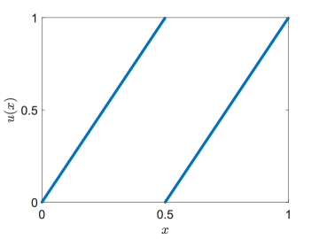 b
b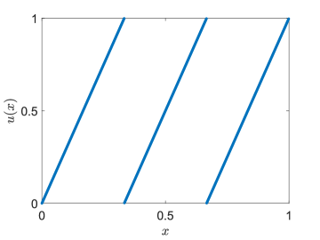
The following simple examples illustrate the relation between the topology of and the structure of solutions of (1.1). Consider the boundary value problem for the Laplace operator on :
| (1.2) |
The only real-valued solutions of (1.2) are constant functions , i.e., up to an additive constant, is a unique solution of (1.2). If on the other hand, takes values in , then there are infinitely many topologically distinct solutions
| (1.3) |
Here, is the degree of the continuous map from to itself. By the Hopf theorem, the degree determines the homotopy class of solutions of -valued solutions of (1.2). Thus, up to translations there is a unique HM from to itself for each homotopy class.
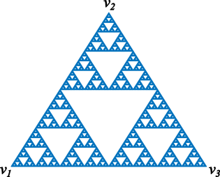
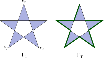
Next we turn to (1.1) on the SG, denoted by : is a unique compact set satisfying the following fixed point equation
| (1.4) |
where
and ’s are vertices of an equilateral triangle (see Fig. 2) [5]. The set will be used to assign the boundary values for the Laplace equation (1.1) on .
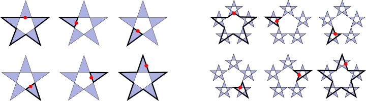
As a fractal domain, has a more interesting topology than the unit circle used in the previous example. Naturally, one expects to find a richer family of HMs from to compared to the HMs from to itself. HMs shown in Figure 3 confirm this intuition.
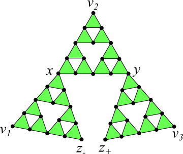
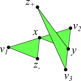
To describe the structure of the HMs from to the circle, we first need to explain the structure of the loop space of . To this end, let stand for a solid closed triangle with vertices and and let stand for the alphabet of three symbols. For and , we define an -cell as
and stands for an oriented boundary of . In addition, .
Let stand for the loops from with taken in lexicographical order, i.e., etc.
a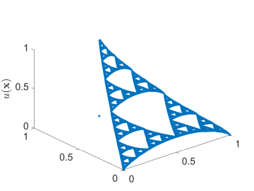 b
b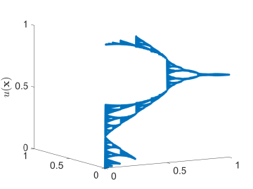 c
c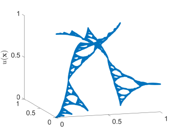 d
d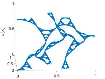
Given , the restriction of to after appropriate reparametrization yields a map from to itself, . Let denote the degree of . The degree of is defined as follows
| (1.5) |
where is the degree of restricted to a closed simple path and reparametrized appropriately. In Section 2, we show that (1.5) determines the homotopy type of as a map from to .
Since is uniformly continuous and the diameter of goes to as the length of goes to infinity, has only finitely many nonzero entries. Consequently, there exists such that the winding numbers for loops bounding -cells for are all zero:
Therefore, the homotopy class of a harmonic map on is determined by the degree over loops bounding -cells for , i.e., by a finite number of entries in (1.5)
| (1.6) |
where we dropped the infinite sequence of zeros at the end.
Theorem 2.6 states that (1.1) on the SG with appropriate boundary conditions has a unique solution from each homotopy class. This shows that like for HMs from to itself, there are infinitely many -valued solutions of the Laplace equation on SG. The hierarchy of HMs on is given by the integer-valued vector (1.5), the degree of . It is known that continuous maps between compact Riemannian manifolds are homotopic to HMs (cf. [4]). Theorem 2.6 implies that like HMs between Riemannian manifolds, HMs from SG to the circle represent homotopy classes of continuous functions. Theorem 2.6 was formulated and proved by Strichartz in 2001 (cf. [13]). It was conjectured in [13] that Theorem 2.6 can be extended to HMs from p.c.f. sets to the circle.
In this paper, we develop a geometric proof of the Strichartz’s theorem, which extends to HMs from p.c.f. fractals to the circle. At the heart of our method lies the construction of a covering space for a given fractal set. The covering space is constructed separately for each homotopy class. With the covering space in hand, we lift -valued continuous function on a fractal to a real-valued continuous function on the covering space. After that we apply the standard harmonic extension algorithm used for computing (real-valued) harmonic functions on p.c.f. fractals (cf. [8]). The desired HM is obtained by restricting the domain of the harmonic function on the covering space to the fundamental domain and projecting the range to the unit circle.
The outline of the paper is as follows. In Section 2, we discuss continuous maps from the SG to the circle. Here, we define the degree of the HM from the SG to the circle and show that it determines the homotopy class like in the case of the maps from a circle to itself. In Section 3, we review relevant facts from the theory of real-valued harmonic functions on the SG. After that we explain the construction of the covering space and the harmonic structure on the covering space in Section 4 and Section 5 respectively. This is followed by the construction of the HM from the SG to the circle in Section 6. For clarity of presentation, we first discuss in detail the case of a simple degree, i.e., when the degree is given by a single integer: . Then we explain how to extend the construction of the covering space for HMs on SG with arbitrary degree in Section 7. Finally, we discuss the generalization of our method to p.c.f. fractals, for which the harmonic extension algorithm is developed in Section 8. Here, we highlight the special features of the SG that were used in the proof of Theorem 2.6, but are no longer available in the more general case of p.c.f. fractals, and propose ways how to overcome this problem.
2 The boundary value problem
Following [13], HMs on SG and other p.c.f. fractals will be constructed as solutions of a certain boundary value problem. Recall that we will denote SG by . To set up the problem for , we need to understand the homotopy classes of continuous functions on first. To this end, let
For each triangular loop , we choose a reference point . For concreteness, let be the leftmost vertex of .
For , we choose a uniform parametrization , which starts at , , and traces in clockwise direction with constant speed.
For a given , is a continuous function from to itself111Throughout this paper, is a uniform parametrization, i.e., .
There is a unique continuous function such that
| (2.1) | ||||
| (2.2) |
The second condition (2.2) can be written as
| (2.3) |
where
is called the lift of . The degree of is expressed in terms of the lift of :
Definition 2.1.
The degree of is defined by
| (2.4) |
where .
Remark 2.2.
Since is uniformly continuous on , the number of nonzero entries in (2.4) is finite.
Definition 2.3.
Two maps are called homotopic, denoted , if there exists a continuous mapping such that
| (2.5) |
Theorem 2.4.
Let . Then if and only if .
Proof.
Suppose . Then there exists satisfying (2.5). Let . Choose a parametrization and consider and . Then and are two continuous maps from to itself. They are homotopic with the homotopy provided by . By the Hopf degree theorem, .
Conversely, suppose . In particular,
| (2.6) |
We claim that
| (2.7) |
provides the desired homotopy between and . The key point is to check that is well defined as a continuous map from to , i.e., for every and
| (2.8) |
The equality in (2.8) clearly holds for . Let be arbitrary but fixed and note
Thus, is a uniformly continuous function on . Since is dense in there is a unique continuous extension of to ∎
We now turn to the Laplace equation
where .
In analogy to the formulation of the Dirichlet problem for real-valued functions on [8, 12], we include the values of on in the formulation of the boundary value problem for HMs. In fact, we need a little more. Note that eventually we will need to recover . Thus, instead of the values of we incorporate the values of , the lift of , to our formulation of the boundary value problem for . Specifically, we use
| (2.9) | ||||
Here, .
Remark 2.5.
In addition to (2.9), in analogy to the case of HMs from to , we will need to specify the homotopy class of :
| (2.10) |
We can now state our main result for the SG.
3 Harmonic structure on SG
Before discussing -valued HMs on , it is instructive to review the definition and basic properties of real-valued harmonic functions on (cf. [8, 14]).
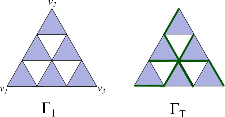
First, we define a family of graphs approximating . Specifically, for , is a graph on nodes. The set of nodes of is denoted by . Two nodes are adjacent (denoted ) if they belong to the same -cell, i.e., for some . Geometrically, (see Fig. 4).

We will distinguish the boundary and interior nodes of . The former are given by the vertices of , i.e., , and the latter are the remaining nodes . Let stand for the space of functions from to .
Definition 3.1.
is called -harmonic if it satisfies the discrete Laplace equation at every interior node of :
| (3.1) |
Harmonic functions on the SG and other fractals are defined with the help of the Dirichlet (energy) form , which in turn is defined using properly scaled energy forms on graphs approximating corresponding fractals (cf. [8]). For , the Dirichlet forms on the sequence of graphs are defined as follows:
| (3.2) |
The sequence of Dirichlet forms has the following properties.
-
1.
A -harmonic minimizes over all functions subject to the same boundary conditions
(3.3) -
2.
The minimum of the energy form over all extensions of to is equal to :
(3.4)
The first property follows from the Euler-Lagrange equation for . This property does not depend on the scaling coefficient in (3.2). The second property, on the other hand, holds due to the choice of the scaling constant . The sequence of equips with a harmonic structure.
By (3.4), forms a non-decreasing sequence for any . Thus,
is well-defined. The domain of the Laplacian on is defined by
Definition 3.2.
A function is called harmonic if it minimizes over all continuous functions on subject to given boundary conditions on .
Property (3.4) yields a recursive algorithm for computing the values of a harmonic function on , a dense subset of . For , the values on are prescribed:
Given the values on are computed using the following rule, which we state for an arbitrary fixed -cell : Suppose the values of at , the nodes of , are known. Then the values of at the nodes at the next level of discretization are computed as follows
| (3.5) |
where stands for the value of at (Figure 5; see [8, 12] for details on harmonic extension).

The recursive algorithm of computing the values of a harmonic function on using its values on via (3.5) is called harmonic extension. Using (3.4), one can show that at each step of the harmonic extension:
| (3.6) |
Thus, each of is a -harmonic function. Further, harmonic extension results in a uniformly continuous function on . Thus, the values of on can be obtained from to SG by continuity (see [12, §11.2] for more details). The continuous function obtained in this way minimizes over all continuous functions on SG with the same boundary conditions. This yields a harmonic function on SG.
By construction, and is also -harmonic for every . This property may be used as an alternative definition of a harmonic function on SG.
4 The covering space
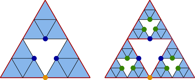
In this section, we explain the construction of covering spaces for , which are the key tool in the proof of Theorem 2.6. The covering space is constructed separately for each degree vector . We begin with the simplest case, In the remainder of this section, we assume that , because otherwise can be computed using the standard harmonic extension algorithm for real valued functions (cf. (3.5)).
Before we turn to the construction of the covering space, we take a slight detour to explain the coding of the nodes of the graphs approximating . Every node from is a vertex of the corresponding triangle and can be represented as
Thus, for each node in we define an itinerary , where stands for the infinite sequence of ’s: . Note that for there are two possible itineraries, e.g., and correspond to the same node from .
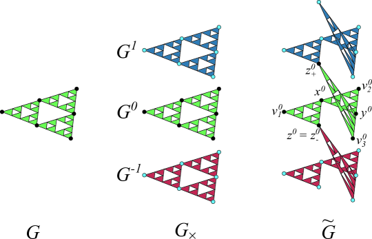
The construction of the covering space involves the following steps.
- 1.
-
2.
Then cut each at , i.e., we replace with two distinct copies
(4.5) -
3.
Identify
(4.6) -
4.
The covering space , is the topological space obtained after identification (4.6). The copies of , belonging to different levels , compose the sheets of . We keep denoting them by . Each sheet contains both copies of and is called the fundamental domain.
-
5.
For , we introduce a family of graphs approximating (see Figure 7). are constructed in the same way as graphs in the previous section (see Figure 4), with the only distinction that replaced with the the two copies and (see Figure 7). By identifying , we obtain the discretization of the covering space , . The set of nodes of is denoted by , , and is dense in
5 Harmonic structure on
Harmonic functions on will be constructed via minimization of the energy form to be defined next. To this end, let and be arbitrary fixed numbers and define
| (5.1) |
for and (see Figure 8).
The energy form on is defined as follows
| (5.2) |
The energy form inherits the key properties of the Dirichlet form (see (3.3), (3.4)):
-
1.
A -harmonic minimizes over :
(5.3) -
2.
The minimum of the energy form over all extensions of to is equal to :
(5.4)
For every , consider the minimization problem
| (5.5) |
Lemma 5.1.
Proof.
Let be arbitrary but fixed.
Since is bounded from below and the sub-level sets are compact, we conclude that (5.5) has at least one solution.
Let be a minimizer of . By (5.4), .
Remark 5.2.
Having found the minimizer on , we extend it by continuity to the fundamental domain , and further to a uniformly continuous function on the covering space:
| (5.7) |
Theorem 5.3.
The restriction of on , , is -harmonic for every :
| (5.8) |
Proof.
By construction, is the unique minimizer of on . Thus, is -harmonic and it remains to check that satisfies the discrete Laplace equation at . It is sufficient to verify this only at .
To simplify the notation, for the reminder of the proof we set . Denote the graph obtained by gluing and by
where for the vertex set of we take the union of the node sets of these two graphs with and keep the adjacency relations from and . Denote the node set of by .
Define by
| (5.9) |
We want to show that is the minimizer of
| (5.10) |
where
This will imply that is -harmonic at , because is an interior point of .
First, note that minimization problem (5.10) has a unique solution (cf. Lemma 5.1), which we denote by
| (5.11) |
Using the symmetry of the energy form, observe that if (5.11) minimizes (5.10) then so does
The uniqueness of the minimizer (5.10) then implies
From this we conclude that and . Thus, (cf., (5.9)), which means that is -harmonic. ∎
6 Simple harmonic maps from SG to
Having constructed , a harmonic function on the covering space, we are one step away from producing a HM on SG. This is done by restricting the domain of to the fundamental domain and by projecting the range of to :
| (6.1) |
Intuitively, it is clear that is the desired HM. In the remainder of this section, we clarify the variational interpretation of this statement, i.e., we show that is a critical point of the appropriate energy functional on . To this end, we need to adapt the definitions of the energy forms and function spaces from the previous section to the present setting.
For we define
| (6.2) |
where is the geodesic distance on .
Recall the definition of from the previous section. Identify to obtain Note that the approximate .
Since is uniformly continuous on , for large enough ,
and thus
This combined with Lemma 5.1 implies that is a unique minimizer of in .
The rest of the argument follows the standard scheme. Using the properties of (cf. (5.4)), we deduce that forms a non-decreasing sequence for any and define
By construction, and
7 Higher order maps
In the previous section, we completed the construction of a HM of a simple degree. In this section, we extend the algorithm for the case of an arbitrary degree.
Let be a HM of degree
| (7.1) |
We say that is a HM of order if
The construction of the covering space for higher order HMs requires additional cuts, which we explain below. To this end, note that the degree of the HM of order can be rewritten as
| (7.2) |
where
For , we choose the same cut points as before
and identify
At step , we have and choose cut point such that it belongs to the boundary of the corresponding -cell, but does not belong to the boundary of the parent -cell (see Figure 9). Formally, , where . Here, stands for the complement of .
Denote the two itineraries of by .
Next, we cut at and identify
| (7.3) |
The cut points for the first, second, and third order HMs are shown in Figure 9 (also see Appendix A for explicit formulae for the cut points needed for construction of the second order HMs).
The remainder of the algorithm proceeds as in Section 5. Specifically, let Then approximate the sheets of by graphs Define discrete spaces
As in Lemma 5.1, one can show that for every
has a unique solution, which can be computed via harmonic extension. By extending this solution to as in (5.7), we obtain a -harmonic function. By repeating this procedure for all , we obtain the values of harmonic , which after restricting to the fundamental domain and projecting to yields the desired HM with the prescribed degree (5.9). Figure 3d shows an example of a HM with degree .
8 Extending to p.c.f. fractals
The goal of this section is to extend the algorithm for constructing HMs to a broader class of fractals. The first step in this direction is to identify necessary assumptions on the self-similar set, which enable such an extension. To this end, in § 8.1, we review the definition of a p.c.f. fractal and a harmonic structure on the p.c.f. fractals following [8, 12]. Subsequently, in § 8.2, we discuss specific features of the SG that are absent in a general p.c.f. set. These differences prompt certain adjustments in our approach to the general case. After discussing the setting and formulating the corresponding assumptions, we present Theorem 8.2, the main result of this section. This is followed by a discussion of several representative examples in § 8.3.
8.1 P.c.f. fractals and harmonic structure
Let be an attractor of an iterated function system, i.e., is compact set satisfying
| (8.1) |
where such that
In addition, we assume that is connected222The ambient Euclidean space is used to simplify presentation. Any other metric space may be used instead [8].
Let and define -cells as before
The critical set of is defined by
Assume that and define
| (8.2) |
Definition 8.1.
Let be a compact connected set satisfying (8.1). is called a p.c.f. fractal if is finite.
For the remainder of this section, we assume that is a p.c.f. fractal.
Let
Note that
as in the case of SG discussed above. Further,
is dense in .
Next, we we equip with a harmonic structure. Specifically, we assume that there is a sequence of quadratic forms
where is a positive definite matrix.
The sequence satisfies the following two conditions:
- i
-
Self-similarity. There exist such that
(8.3) - ii
-
Compatibility. For every
(8.4)
The compatibility condition implies that is non-decreasing for any . Thus,
is well-defined and
Furthermore, thanks to (8.4), the minimization problem
can be solved recursively
This is the basis of the harmonic extension algorithm.
The harmonic structure implicitly defines a sequence of graphs approximating :
8.2 The main result
For a general p.c.f. self-similar set , unlike SG, there is no natural candidate for the basis of the cycle space of a graph approximating (see, e.g., 3-level SG in Figure 11). Likewise, the outer boundary of used for assigning the condition for the lift (2.10) may be much more complicated than that for the SG (see, e.g., the hexagasket in Figure 13). These observations motivate a slightly different approach to formulating the boundary value problem for the HM on . Below we formulate the necessary assumptions and state the main result concerning the existence of HMs from a general p.c.f. set to the circle.
Let be a graph approximating at level . To formulate the analog of (2.9)-(2.10), we pick a basis for the cycle space of , :
| (8.5) |
For let stand for the set of vertices forming
Further, we embed the cycles from to , , such that
| (8.6) |
and
| (8.7) |
We also assume that for every there is such that
| (8.8) |
We postulate the existence of the embedding and satisfying (8.6), (8.7) and (8.8) respectively. These assumptions are used in the construction of the covering space for .
We are now ready to formulate the boundary value problem for HMs in general. Following the strategy developed for the SG, to construct HMs on p.c.f. fractals we formulate the boundary value problem for a harmonic function on the fundamental domain of the covering space. To this end, fix a level and the degree
| (8.9) |
where is the degree of .
Let be a cycle that contains boundary vertices . Here, by abuse of notation also stands for the corresponding loop in . We impose the analog of (2.9):
| (8.10) | ||||
where and
Proof.
The key constructions and the corresponding results in Sections 4-7 translate to the present setting with minor modifications, so we highlight only the main distinctions from the previous proof for SG.
First, denote the trivial covering space . As described above, embed the cycles into . For each , fix a cut point disjoint from the other embedded cycles , . Finally, make the following identifications in the covering space:
where stand for the two itineraries of along the cycle , cf. (7.3). The resultant space is comprised of sheets , and has associated graphs with vertices . As before approximates the fundamental domain.
The remainder of the procedure is implemented similarly. Define the discrete spaces with appropriate boundary and jump conditions:
and energy form
| (8.11) |
Repeating the energy minimization along the lines of Lemma 5.1 results in a unique harmonic function on . This can be harmonically extended as in Lemma 5.3 to a dense set of , and further extended by uniform continuity to obtain a harmonic function on the entire . Restricting to the fundamental domain and projecting the range to yields the desired harmonic map. ∎
8.3 Examples
The following examples are meant to illustrate key steps in the construction of the covering space for a set of representative p.c.f. fractals. With the covering space in hand, the rest of the algorithm follows as discussed in Theorem 8.2.
For each of the following examples, we use a simple method for generating the required basis and associated cut points. Begin with a spanning tree, of . Adding any edge, , not contained in generates a cycle; the collection of all such cycles forms a basis [3]. The cut points are constructed using the same edges, . For each edge, simply select any vertex along the embedded image of in .
8.4
The level- SG generalizes the SG [8]. Take to be the vertices of a triangle . The is constructed via an iterated function system by defining maps
where
Taking results again in SG. For the are generated by the expressions
Figure 10 shows and a corresponding spanning tree for . Figure 11 shows the associated cycle basis and locations of cut points.
In contrast to , the boundaries no longer form a basis for the cycle space of . Indeed, we see , while for the cycle space is in fact -dimensional. HMs at this level.
a)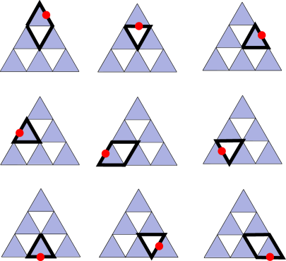 b)
b) 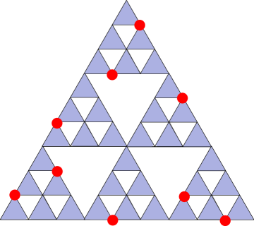
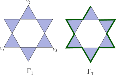
8.5 Polygaskets
Polygaskets generalize the construction of SG to regular polygons. Consider a regular -gon, , with not divisible by 4. Then define homotheties with fixed points the vertices of such that and intersect at a single point when . As discussed in [14], one can compose the with rotations so that it is sufficient to take as the boundary just 3 vertices of the -gon: .
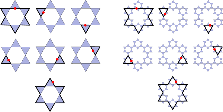
Figures 12 and 13 demonstrate the construction of the cycle basis and cut points for the first level of the hexagasket (this fractal was also studied in [15] following the method of [13]). Like the , edges in the hexagasket embed naturally from to , making the identification of cycles and cut points in relatively straightforward.
In contrast, Figures 14 and 15 show the pentagasket. In this case, there is a non-trivial embedding of cycles from to . Nonetheless, it is still possible to construct a cycle basis and cut points in satisfying (8.6)-(8.8).
9 Discussion
In this paper, we presented a method for constructing HMs from the p.c.f. fractals to the unit circle using the covering spaces for the underlying fractal. The method provides a complete description of HMs from the SG to the unit circle. Specifically, it shows that there is a unique HM satisfying given boundary conditions in each homotopy class. In addition, the method yields explicit and exact formulae for computing HMs on a dense set of points. Our method may be viewed as a natural generalization of the classical harmonic extension algorithm for real-valued functions (cf. [8]; see also [14, 12]).
The method extends naturally to a large class of fractals, the p.c.f. fractals. While the implementation of the computational algorithm and the proof of the main result remain practically the same as in the case of SG, the analysis of the HMs on p.c.f. sets reveals subtle differences. Namely, for SG the cycle spaces of approximating graphs embed nicely from one level approximation to the next one. This affords an especially nice and simple way of describing the degree of a HM on SG (see (2.10)). Examples of level- SG and polygaskets show that in general the relation between cycles spaces of approximating graphs at different levels of approximation may be more complex. This prevented us from claiming uniqueness in Theorem 8.2, even though the gist of the matter remained the same as before. By construction, the HM obtained in the proof of Theorem 8.2 is still unique in a given homotopy class, provided the latter is fully captured by (8.9), i.e., there are no nonzero winding numbers at smaller scales. For SG, this condition was conveniently expressed by the nonzero entries of (2.10) or by the order of the HM. While the meaning of the order of HM is intuitively clear for a general p.c.f. set, expressing it formally meets certain technical difficulties, which are postponed for a future study. Nonetheless, the covering spaces for p.c.f. fractals that we introduced in this work provide a nice visual tool for describing the geometry of HMs to the unit circle and we believe that they will find other interesting applications.
Acknowledgments. The work of both authors is partially supported by NSF.
Appendix A Appendix: Cut points for SG
-
1.
As before we cut every at :
and identify .
-
2.
In addition, for every and .
-
(a)
Denote
-
(b)
Cut at and :
-
(c)
Identify
where
-
(a)
References
- [1] Martin T. Barlow, Diffusions on fractals, Lectures on probability theory and statistics (Saint-Flour, 1995), Lecture Notes in Math., vol. 1690, Springer, Berlin, 1998, pp. 1–121.
- [2] Martin T. Barlow and Edwin A. Perkins, Brownian motion on the Sierpiński gasket, Probab. Theory Related Fields 79 (1988), no. 4, 543–623.
- [3] Reinhard Diestel, Graph theory, Springer (print edition); Reinhard Diestel (eBooks), 2024.
- [4] James Eells, Jr. and J. H. Sampson, Harmonic mappings of Riemannian manifolds, Amer. J. Math. 86 (1964), 109–160.
- [5] Kenneth Falconer, Fractal geometry, third ed., John Wiley & Sons, Ltd., Chichester, 2014, Mathematical foundations and applications.
- [6] Sheldon Goldstein, Random walks and diffusions on fractals, Percolation theory and ergodic theory of infinite particle systems (Minneapolis, Minn., 1984–1985), IMA Vol. Math. Appl., vol. 8, Springer, New York, 1987, pp. 121–129.
- [7] Jun Kigami, Harmonic calculus on p.c.f. self-similar sets, Trans. Amer. Math. Soc. 335 (1993), no. 2, 721–755.
- [8] , Analysis on fractals, Cambridge Tracts in Mathematics, vol. 143, Cambridge University Press, Cambridge, 2001.
- [9] Shigeo Kusuoka, A diffusion process on a fractal, Probabilistic methods in mathematical physics (Katata/Kyoto, 1985), Academic Press, Boston, MA, 1987, pp. 251–274.
- [10] Georgi S. Medvedev, Galerkin approximation of a nonlocal diffusion equation on euclidean and fractal domains, arXiv:2306.15844, 2023.
- [11] Georgi S. Medvedev and Matthew S. Mizuhara, in preparation.
- [12] Ricardo A. Sáenz, Introduction to harmonic analysis, Student Mathematical Library, vol. 105, American Mathematical Society, Providence, RI; Institute for Advanced Study (IAS), Princeton, NJ, [2023] ©2023, IAS/Park City Mathematical Subseries.
- [13] Robert S. Strichartz, Harmonic mappings of the Sierpinski gasket to the circle, Proc. Amer. Math. Soc. 130 (2002), no. 3, 805–817. MR 1866036
- [14] , Differential equations on fractals, Princeton University Press, Princeton, NJ, 2006, A tutorial.
- [15] Donglei Tang, Harmonic mappings of the hexagasket to the circle, Anal. Theory Appl. 27 (2011), no. 4, 377–386.