Dynamic Subgraph Matching via Cost-Model-based Vertex Dominance Embeddings (Technical Report)

Abstract.

In many real-world applications such as social network analysis, knowledge graph discovery, biological network analytics, and so on, graph data management has become increasingly important and has drawn much attention from the database community. While many graphs (e.g., Twitter, Wikipedia, etc.) are usually involving over time, it is of great importance to study the dynamic subgraph matching (DSM) problem, a fundamental yet challenging graph operator, which continuously monitors subgraph matching results over dynamic graphs with a stream of edge updates. To efficiently tackle the DSM problem, we carefully design a novel vertex dominance embedding approach, which effectively encodes vertex labels that can be incrementally maintained upon graph updates. Inspire by low pruning power for high-degree vertices, we propose a new degree grouping technique over basic subgraph patterns in different degree groups (i.e., groups of star substructures), and devise degree-aware star substructure synopses (DAS³) to effectively facilitate our designed vertex dominance and range pruning strategies. We develop efficient algorithms to incrementally maintain dynamic graphs and answer DSM queries. Through extensive experiments, we confirm the efficiency of our proposed approaches over both real and synthetic graphs.

PVLDB Reference Format:
PVLDB, 14(1): XXX-XXX, 2020.
doi:XX.XX/XXX.XX

PVLDB Artifact Availability:
The source code, data, and/or other artifacts have been made available at https://github.com/JamesWhiteSnow/DSM.

1. Introduction

For the past few decades, the subgraph matching problem has been extensively studied as a fundamental operator in the graph data management (Orogat and El-Roby, 2022; Wasserman and Faust, 1994; Karlebach and Shamir, 2008; Szklarczyk et al., 2015; Chen et al., 2009; Zhang and Yu, 2022) for many real-world applications such as social network analysis, knowledge graph discovery, and pattern matching in biological networks. Given a large-scale data graph $G$, a subgraph matching query finds all the subgraphs of $G$ that are isomorphic to a given query graph $q$.

While many previous works (He and Singh, 2008; Shang et al., 2008; Bonnici et al., 2013; Bi et al., 2016; Jüttner and Madarasi, 2018; Han et al., 2019; Bhattarai et al., 2019; Sun and Luo, 2020) usually considered the subgraph matching over static graphs, real-world graph data are often dynamic and change over time. For example, in social networks, friend relationships among users may be subject to changes (e.g., adding or breaking up with friends); similarly, in collaboration networks, people may start to collaborate on some project and then suddenly stop the collaboration for years. In these scenarios, it is important, yet challenging, to conduct the subgraph matching over such a large-scale, dynamic data graph $G_{D}$, upon updates (e.g., edge insertions/deletions). In other words, we need to continuously monitor subgraphs (e.g., user communities or collaborative teams) in $G_{D}$ that follow query graph patterns $q$.

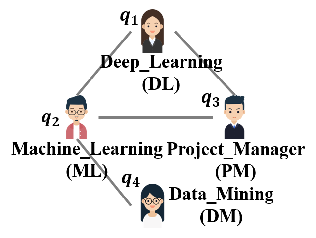
(a) query graph $q$

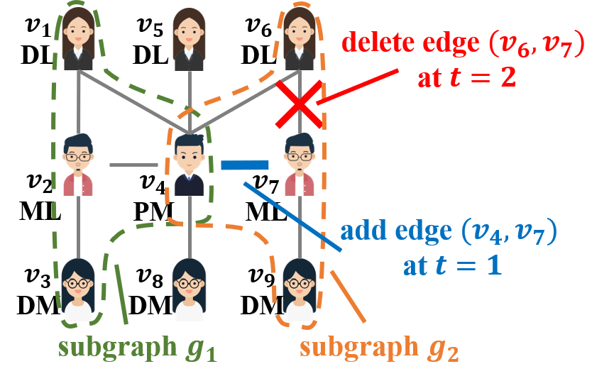
(b) dynamic collaboration network $G_{D}$

Figure 1. An example of the subgraph matching in dynamic collaboration networks $G_{D}$.

Below, we give an example of the subgraph matching over dynamic collaboration networks in the expert team search application.

Example 0.

(Monitoring Project Teams in Dynamic Collaboration Networks (Fan et al., 2013a)) Due to numerous requests from departments/companies for recruiting (similar) project teams, a job search advisor may want to monitor the talent market (especially teams of experts) in dynamically changing collaboration networks.

Consider a toy example of a collaboration network $G_{D}$ in Figure 1. Figure 1(a) shows a desirable expert team pattern $q$, which is represented by a graph of 4 experts $q_{1}$$\sim$$q_{4}$, where each expert vertex $q_{i}$ is associated with one’s skill/role keyword (e.g., $q_{1}$ with keyword “Deep_Learning” and $q_{3}$ with “Project_Manager”), and each edge indicates that two experts had the collaboration before (e.g., edge $(q_{1},q_{3})$).

Figure 1(b) provides an example of a dynamic collaboration network $G_{D}$, where edges are inserted or deleted over time. For example, a new edge $(v_{4},v_{7})$ is inserted at timestamp $t=1$, implying that two experts $v_{4}$ and $v_{7}$ start to collaborate with each other in a team. Similarly, at timestamp $t=2$, an existing edge $(v_{6},v_{7})$ is removed from the graph $G_{D}$, which may indicate that experts $v_{6}$ and $v_{7}$ have not collaborated with each other for a certain period of time (e.g., two years).

In this example, the job search advisor can register a dynamic subgraph matching query over $G_{D}$ to continuously identify subgraphs of $G_{D}$ that match with the query graph pattern $q$. At timestamp $t=1$, subgraphs $g_{1}$ and $g_{2}$ are the subgraph matching answers, whereas at timestamp $t=2$, subgraph $g_{1}$ is the only answer (since the deletion of edge $(v_{6},v_{7})$ invalidates the subgraph $g_{2}$).  $\blacksquare$

Dynamic subgraph matching has many other real applications. For example, in the application of anomaly detection for online shopping (Qiu et al., 2018), the interactions (e.g., purchases, views, likes, etc.) among users/products over time form a dynamic social/transaction graph, and it is important to detect some abnormal events such as fraudulent activities (i.e., query graph patterns) over such a dynamically changing graph.

Inspired by the examples above, we formulate a dynamic subgraph matching (DSM) query over a dynamic graph, which continuously monitors subgraph matching results, upon updates to the data graph.

Prior Works: Due to NP-completeness of the subgraph isomorphism (Garey and Johnson, 1983; Cordella et al., 2004; Grohe and Schweitzer, 2020), dynamic subgraph matching is not tractable. To tackle this problem, several exact algorithms have been proposed (Fan et al., 2013b; Choudhury et al., 2015; Kankanamge et al., 2017; Idris et al., 2017, 2020; Kim et al., 2018; Min et al., 2021), which consist of three categories: recomputation-based (Fan et al., 2013b), direct-incremental (Kankanamge et al., 2017), and index-based incremental algorithms (Choudhury et al., 2015; Idris et al., 2017, 2020; Kim et al., 2018; Min et al., 2021). The recomputation-based algorithms re-compute all the subgraph matching answers at each timestamp from scratch, the direct-incremental algorithms incrementally calculate new matching results from dynamic graphs upon updates, and index-based incremental ones incrementally maintain matching results via auxiliary indexes built over query answers.

Our Contributions: Our work falls into the category of the direct-incremental algorithm. Different from existing works that directly use structural information (e.g., vertex label and neighbors’ label set) to filter out vertex candidates, we design a novel and effective vertex dominance embedding technique for candidate vertex/subgraph retrieval. Specifically, our proposed vertex dominance embeddings can be incrementally maintained in dynamic graphs, and transform our DSM problem into a dominating region search problem in the embedding space with no false dismissals. To enhance the pruning power of our embeddings for high-degree vertices, we propose a new degree grouping approach for vertex embeddings over basic subgraph patterns in different degree groups (i.e., groups of star substructures). We also devise a cost model to further guide the vertex embeddings to effectively achieve high pruning power. Finally, we develop algorithms to incrementally maintain dynamic graphs and answer DSM queries efficiently.

Specifically, in this paper, we make the following contributions:

1. We formally define the dynamic subgraph matching (DSM) problem in Section 2, and propose a general framework for DSM query answering in Section 3.

2. We carefully design incremental vertex dominance embeddings to facilitate dynamic subgraph matching in Section 4.

3. We devise a degree grouping technique to enhance the pruning power of vertex embeddings, and construct degree-aware star substructure synopses (DAS³) to support the dynamic subgraph matching in Section 5.

4. We design effective synopsis pruning strategies, and develop efficient DSM processing algorithms in Section 6.

5. We present a novel cost-model-guided vertex embeddings to further improve the pruning power in Section 7.

6. We demonstrate through extensive experiments the efficiency and effectiveness of our DSM processing algorithm over real/synthetic graphs in Section 8.

Section 9 reviews previous works on dynamic graph management and graph embeddings. Finally, Section 10 concludes this paper.

Table 1. Symbols and Descriptions

Symbol	Description
$G$	a static graph
$G_{D}$	a dynamic graph
$\Delta G_{t}$	a set of graph updates at timestamp $t$
$G_{t}$	a snapshot graph of $G_{D}$ at timestamp $t$
$e+$ (or $e-$)	an insertion (or deletion) of edge $e$
$q$	a query graph
$Q$	a set of query graph patterns
$x_{i}$	a SPUR vector of vertex $v_{i}$
$y_{i}$	a SPAN vector of vertex $v_{i}$’s 1-hop neighbors
$o(v_{i})$ (or $o(g_{v_{i}})$, $o(s_{v_{i}})$)	a vertex dominance embedding vector

2. Problem Definition

Table 1 depicts the commonly used symbols in this paper.

2.1. Static Graph Model

We give the model of a static undirected, vertex-labeled graph $G$.

Definition 0.

(Static Graph, $G$) A static graph, $G$, is denoted as a triple $(V(G),E(G),L(G))$, where $V(G)$ is a set of vertices $v_{i}$, $E(G)$ is a set of edges $e_{i,j}=(v_{i},v_{j})$ between vertices $v_{i}$ and $v_{j}$, and $L(G)$ is a label function from each vertex $v_{i}\in V(G)$ to a label $l(v_{i})$.  $\blacksquare$

The static graph model (as given in Definition 2.1) has been widely used in various real-life applications to reflect relationships between different entities, for example, social networks (Al-Baghdadi et al., 2020), Semantic Web (Hassanzadeh et al., 2012), transportation networks (Rai and Lian, 2023), biological networks (Kan et al., 2023), citation networks (Yang and Han, 2023), and so on.

The Graph Isomorphism: Next, we define the classic graph isomorphism problem between two graphs.

Definition 0.

(Graph Isomorphism) Given two graphs $G_{1}$ and $G_{2}$, graph $G_{1}$ is isomorphic to graph $G_{2}$ (denoted as $G_{1}\equiv G_{2}$), if there exists a bijection mapping function $M:V(G_{1})\Rightarrow V(G_{2})$, such that: i) $\forall v_{i}\in V(G_{1})$, we have $L(v_{i})=L(M(v_{i}))$, and; ii) $\forall e_{i,j}\in E(G_{1})$, edge $e_{M(v_{i}),M(v_{j})}=(M(v_{i}),M(v_{j}))\in E(G_{2})$ holds.  $\blacksquare$

In Definition 2.2, the graph isomorphism problem checks whether graphs $G_{1}$ and $G_{2}$ exactly match with each other.

The Subgraph Matching Problem: The subgraph isomorphism (or subgraph matching) problem is defined as follows.

Definition 0.

(Subgraph Matching) Given graphs $G$ and $g$, a subgraph matching problem identifies subgraphs $g^{\prime}$ of $G$ (i.e., $g^{\prime}\subseteq G$) such that $g$ and $g^{\prime}$ are isomorphic.  $\blacksquare$

Note that, the subgraph matching problem is NP-complete (Garey and Johnson, 1983).

2.2. Dynamic Graph Model

Real-world graphs are often continuously evolving and updated. Examples of such dynamic graphs include social networks with updates of friend relationships among users, bibliographical networks with new collaboration relationships, and so on. In this subsection, we provide the data model for dynamic graphs with update operations below.

Definition 0.

(Dynamic Graph, $G_{D}$) A dynamic graph, $G_{D}$, consists of an initial graph $G_{0}$ (as given by Definition 2.1) and a sequence of graph update operations $\Delta\mathcal{G}=\{\Delta G_{1},\Delta G_{2},\dots,\Delta G_{t},\dots\}$ on $G$. Here, $\Delta G_{t}$ is a graph update operator, in the form of $(e+,t)$ or $(e-,t)$, which indicates either an insertion ($+$) or a deletion ($-$) of an edge $e$ at timestamp $t$, respectively.   $\blacksquare$

Snapshot Graph, $G_{t}$: From Definition 2.4, after applying to initial graph $G$ all the graph update operations up to the current timestamp $t$ (i.e., $\Delta G_{1}$, $\Delta G_{2}$, $\dots$, and $\Delta G_{t}$), we can obtain a snapshot of the dynamic graph $G_{D}$, denoted as $G_{t}$.

Discussions on the Edge Insertion: For the edge insertion $(e+,t)$ in Definition 2.4, there are three cases:

• both ending vertices of $e$ exist in the graph snapshot $G_{t-1}$;

• one ending vertex of $e$ exists in $G_{t-1}$ and the other one is a new vertex, and;

• both ending vertices of $e$ are new vertices.

We will later discuss how to deal with the three cases of edge insertions above for dynamic graph maintenance and incremental query answering.

2.3. Dynamic Subgraph Matching Queries

In this subsection, we define a dynamic subgraph matching (DSM) query in a large dynamic graph $G_{D}$, which continuously monitors subgraph matching answers for a set, $Q$, of query graph patterns.

Definition 0.

(Dynamic Subgraph Matching, DSM) Given a dynamic graph $G_{D}$, a set, $Q$, of query graph patterns $q$, and a timestamp $t$, a dynamic subgraph match (DSM) query maintains a subgraph matching answer set $A(q,t)$ for each query graph pattern $q\in Q$, such that any subgraph $g\in A(q,t)$ in $G_{D}$ is isomorphic to the query graph $q$ (denoted as $g\equiv q$).

Alternatively, for each $q\in Q$, the DSM problem incrementally computes an update, $\Delta A(q,t)$, to the answer set $A(q,t-1)$, upon the change $\Delta G_{t}$ to $G_{t-1}$. $\blacksquare$

In Definition 2.5, the DSM query continuously maintains a subgraph matching answer set $A(q,t)$ (w.r.t. each query graph pattern $q\in Q$) over dynamic graph $G_{D}$ (upon incremental updates) for a long period of time. The DSM problem is quite useful in real applications such as cyber-attack event detection and credit card fraud monitoring.

2.4. Challenges

The subgraph matching problem in a data graph has been proven to be NP-complete (Garey and Johnson, 1983). Thus, it is even more challenging to design effective techniques for answering subgraph matching queries in the scenario of dynamic graphs. Due to frequent updates to the data graph, it is non-trivial how to effectively maintain a large-scale dynamic graph that can support effectively obtaining initial subgraph matching results, and continuously and efficiently monitor DSM answer sets, upon fast graph updates.

To tackle the DSM problem, in this paper, we will propose a novel and effective vertex dominance embedding technique over dynamic graphs, which transforms the subgraph matching to a dominance search problem in a graph-node-embedding space. Our proposed embedding technique can guarantee the subgraph matching with no false dismissals. Furthermore, we also design effective pruning, indexing, and incremental maintenance mechanisms to facilitate efficient and scalable dynamic subgraph matching.

Input: i) a dynamic data graph $G_{D}$; ii) a set, $Q$, of registered query graph patterns, and; iii) current timestamp $t$

Output: the subgraph matching answer set, $A(q,t)$, for each registered query graph $q\in Q$

1

// Graph Maintenance Stage

2

3generate a vertex dominance embedding vector $o(v_{i})$ for each vertex $v_{i}\in G_{0}$

4

5build $m$ synopses, $Syn_{j}$, over vertex embeddings with degree grouping

6

7for each graph update $\Delta G_{t}\in\Delta\mathcal{G}$ do

8       obtain $G_{t}$ by applying the graph update $\Delta G_{t}$ over $G_{t-1}$

9      

10      maintain synopses $Syn_{j}$ by updating the corresponding vertex embeddings

11      

12

// DSM Query Answering

13

// Initial Subgraph Matching Answer Set Generation

14

15for each query graph $q\in Q$ do

16       compute a query embedding vector $o(q_{i})$ of each vertex $q_{i}\in V(q)$

17      

18      find candidate vertex sets $q_{i}.cand\_set$ for query vertices $q_{i}$ by accessing synopses $Syn_{j}$

19      

20      enumerate candidate subgraphs $g$ from candidate vertices in $q_{i}.cand\_set$

21      

22      obtain an initial subgraph matching answer set, $A(q,t)$, of matching subgraphs $g$ ($\equiv q$)

23      

24

// Continuous Subgraph Matching Answer Set Monitoring

25

26for each graph update $\Delta G_{t}\in\Delta\mathcal{G}$ do

27       for each query graph $q\in Q$ do

28            

29            update candidate vertex sets $q_{i}.cand\_set$ by checking the updated vertices in $\Delta G_{t}$

30            

31            compute answer changes $\Delta A(q,t)$ from the new candidate sets $q_{i}.cand\_set$

32            

33            apply changes $\Delta A(q,t)$ to $A(q,t-1)$ and obtain the latest subgraph answers in $A(q,t)$

34            

35            return $A(q,t)$

36            

37      

Algorithm 1 The Dynamic Subgraph Matching Framework

3. The Dynamic Subgraph Matching Framework

In this section, we illustrate a general framework for dynamic subgraph matching in Algorithm 1, which consists of two stages, graph maintenance and DSM query answering stages.

Specifically, in the graph maintenance stage, we first pre-process initial graph $G_{0}$, by constructing a set of $m$ graph synopses, $Syn_{j}$, over vertex dominance embeddings $o(v_{i})$ with $m$ degree groups, respectively (lines 1-2). Then, for each graph update operation $\Delta G_{t}\in\Delta\mathcal{G}$, we incrementally maintain the dynamic graph $G_{t}$ and synopses $Syn_{j}$ (lines 3-5).

In the DSM query answering stage, for each newly registered query graph $q$, we obtain the initial query answer set over the current snapshot $G_{t}$ of the dynamic graph $G_{D}$ (lines 6-10). Then, we monitor the updates in query answer sets over continuously changing dynamic graph $G_{t}$ (lines 11-16).

In particular, for initial answer set generation, we compute query vertex embeddings $o(q_{i})$ from vertices $q_{i}\in V(q)$ in each query graph $q$ (lines 6-7). Then, for each query vertex $q_{i}$, we find and store candidate vertices in a set $q_{i}.cand\_set$ by accessing $Syn_{j}$ (line 8). After that, we enumerate candidate subgraphs $g$ by assembling candidate vertices in $q_{i}.cand\_set$ (line 9), and refine/return matching subgraphs $g$ in an initial subgraph matching answer set $A(q,t)$ (line 10).

Next, to answer the DSM query, for each graph update operation $\Delta G_{t}\in\Delta\mathcal{G}$ and each query graph $q\in Q$, we check the updated vertices in $\Delta G_{t}$, update candidate vertex sets $q_{i}.cand\_set$, and monitor the changes $\Delta A(q,t)$ in $A(q,t)$ (lines 11-14). Finally, we obtain $A(q,t)$ by applying changes $\Delta A(q,t)$ to $A(q,t-1)$, and return $A(q,t)$ as the DSM query answer set (lines 15-16).

4. Incremental Vertex Dominance Embeddings

In this section, we will present our vertex dominance embeddings, which can be incrementally maintained, preserve dominance relationships between basic subgraph patterns (i.e., star subgraphs), and support efficient subgraph matching over dynamic graphs.

4.1. Preliminaries and Terminologies

We first introduce two terms of basic subgraph patterns (used for our proposed vertex dominance embedding), that is, unit star subgraphs and star substructures:

• Unit Star Subgraph $g_{v_{i}}$: A unit star subgraph $g_{v_{i}}$ is defined as a (star) subgraph in $G_{t}$ containing a center vertex $v_{i}$ and its one-hop neighbors.

• Star Substructure $s_{v_{i}}$: A star substructure $s_{v_{i}}$ is defined as a (star) subgraph of the unit star subgraph $g_{v_{i}}$ in $G_{t}$ (i.e., $s_{v_{i}}\subseteq g_{v_{i}}$), which shares the same center vertex $v_{i}$.

As an example in Figure 2(a), the unit star subgraph $g_{v_{1}}$ in data graph $G_{t}$ contains a center vertex $v_{1}$ and its 1-hop neighbors $v_{2}$, $v_{3}$, and $v_{4}$. Figure 2(b) illustrates 8 ($=2^{3}$) possible star substructures $s_{v_{1}}$ ($\subseteq g_{v_{1}}$), which are centered at vertex $v_{1}$ and with different combinations of $v_{1}$’s 1-hop neighbors.

4.2. Vertex Dominance Embedding

In this subsection, we discuss how to obtain an embedding vector, $o(v_{i})$, for each vertex $v_{i}$, which embeds labels of vertex $v_{i}$ and its 1-hop neighbors (i.e., unit star subgraph or star substructure). Specifically, the embedding vector $o(v_{i})$ consists of two portions, a Seeded PseUdo Random (SPUR) vector $x_{i}$ and a SPUR Aggregated Neighbor (SPAN) vector $y_{i}$.

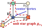
(a) unit star subgraph $g_{v_{1}}$

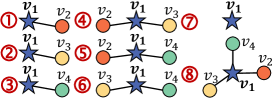
(b) 8 possible star substructures $s_{v_{1}}$

Figure 2. Illustration of unit star subgraph and star substructures.

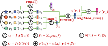
Figure 3. Illustration of vertex dominance embedding $o(v_{1})$ and the optimized vertex dominance embedding $o^{\prime}(v_{1})$.

Seeded PseUdo Random (SPUR) Vector, $x_{i}$: In the dynamic graph $G_{D}$, each vertex $v_{i}$ is associated with a label $l(v_{i})$, which can be encoded by a nonnegative integer. By treating the vertex label $l(v_{i})$ as the seed, we can generate a Seeded PseUdo Random (SPUR) vector, $x_{i}$, of arity $d$ via a pseudo-random number generator $f_{1}(\cdot)$. That is, we have:

(1) $$x_{i}=f_{1}(l(v_{i})).$$

We denote $x_{i}[j]$ as the $j$-th element in SPUR vector $x_{i}$, where $1\leq j\leq d$ and $x_{i}[j]>0$.

Note that, since our randomized SPUR vector $x_{i}$ is generated based on the seed (i.e., label $l(v_{i})$ of each vertex $v_{i}$), vertices with the same label will have the same SPUR vector.

In the example of Figure 3, vertices $v_{1}\sim v_{4}$ are associated with labels $l(v_{1})\sim l(v_{4})$, respectively. We generate their corresponding SPUR vectors, $x_{1}\sim x_{4}$, via a randomized function $f_{1}(\cdot)$ in Eq. (1).

SPUR Aggregated Neighbor (SPAN) Vector, $y_{i}$: Next, for each vertex $v_{i}$, we consider its 1-hop neighbors, $v_{j}\in\mathcal{N}_{v_{i}}$, in a star subgraph pattern (i.e., the unit star subgraph $g_{v_{i}}$ or star substructure $s_{v_{i}}$), and sum up their corresponding SPUR vectors $x_{j}$ to generate a SPur Aggregated Neighbor (SPAN) vector $y_{i}$:

(2) $$y_{i}=\sum_{\forall v_{j}\in\mathcal{N}_{v_{i}}}x_{j},$$

where $\mathcal{N}_{v_{i}}$ is a set of 1-hop neighbors of $v_{i}$, and $x_{j}$ are the SPUR vectors of 1-hop neighbors of $v_{i}$.

Taking Figure 3 as an example, the SPAN vector of the vertex $v_{1}$ is calculated by $y_{1}=x_{2}+x_{3}+x_{4}$.

Vertex Dominance Embedding, $o(v_{i})$: We define the vertex dominance embedding vector, $o(v_{i})$, of each vertex $v_{i}$, by concatenating its SPUR vector $x_{i}$ and SPAN vector $y_{i}$:

(3) $$o(v_{i})=x_{i}\text{ }||\text{ }y_{i},$$

where $||$ is the concatenation operation of two vectors, and $x_{i}$ and $y_{i}$ are given in Eqs. (1) and (2), respectively.

Intuitively, vertex dominance embedding $o(v_{i})$ encodes label features of a star subgraph pattern (i.e., $g_{v_{i}}$ or $s_{v_{i}}$) containing center vertex $v_{i}$ and its 1-hop neighbors. To distinguish vertex dominance embeddings $o(v_{i})$ from different star subsgraph patterns, we also use notations $o(g_{v_{i}})$ or $o(s_{v_{i}})$.

As shown in Figure 3, the vertex dominance embedding of vertex $v_{1}$ can be computed by $o(v_{1})=x_{1}\text{ }||\text{ }y_{1}$.

4.3. Properties of Vertex Dominance Embedding

The Dominance Property of Vertex Embeddings: From Eq. (3), the vertex dominance embedding $o(v_{i})$ is a combination of SPUR and SPAN vectors. Given any unit star subgraph $g_{v_{i}}$ and its star substructure $s_{v_{i}}$ (i.e., $s_{v_{i}}\subseteq g_{v_{i}}$), their vertex dominance embeddings always satisfy the dominance (Borzsony et al., 2001) (or equality) condition: $o(s_{v_{i}})[j]\leq o(g_{v_{i}})[j]$, for all dimensions $1\leq j\leq 2d$, which is denoted as $o(s_{v_{i}})\preceq o(g_{v_{i}})$ (including the case where $o(s_{v_{i}})=o(g_{v_{i}})$).

The reason for the property above is as follows. Since star patterns $s_{v_{i}}$ and $g_{v_{i}}$ have the same center vertex $v_{i}$, the vertex embeddings, $o(s_{v_{i}})$ and $o(g_{v_{i}})$, for $s_{v_{i}}$ and $g_{v_{i}}$, respectively, must share the same SPUR vector $x_{i}$. Moreover, since $s_{v_{i}}\subseteq g_{v_{i}}$ holds, 1-hop neighbors of vertex $v_{i}$ in $s_{v_{i}}$ and $g_{v_{i}}$ must satisfy the condition that $\mathcal{N}_{v_{i}}(s_{v_{i}})\subseteq\mathcal{N}_{v_{i}}(g_{v_{i}})$. As the SPAN vectors are defined as the summed SPUR aggregates of 1-hop neighbors in $\mathcal{N}_{v_{i}}(s_{v_{i}})$ and $\mathcal{N}_{v_{i}}(g_{v_{i}})$, respectively, we have the dominance relationship between SPAN vectors $y_{i}(s_{v_{i}})$ and $y_{i}(g_{v_{i}})$ (i.e., $y_{i}(s_{v_{i}})\preceq y_{i}(g_{v_{i}})$).

Lemma 4.1.

(The Dominance Property of Vertex Embeddings) Given a unit star subgraph $g_{v_{i}}$ centered at vertex $v_{i}$ and any of its star substructures $s_{v_{i}}$ (i.e., $s_{v_{i}}\subseteq g_{v_{i}}$), their vertex dominance embeddings satisfy the condition that: $o(s_{v_{i}})\preceq o(g_{v_{i}})$ (including $o(s_{v_{i}})=o(g_{v_{i}})$) in the embedding space.

Proof.

For a given unit star subgraph $g_{v_{i}}$ centered at vertex $v_{i}$ and any of its star substructures $s_{v_{i}}$ (i.e., $s_{v_{i}}\subseteq g_{v_{i}}$), since they share the same center vertex $v_{i}$ (i.e., with the same label $l(v_{i})$), they must have the same SPUR vector $x_{i}$.

Moreover, since $s_{v_{i}}\subseteq g_{v_{i}}$ holds, we also have $\mathcal{N}_{v_{i}}(s_{v_{i}})\subseteq\mathcal{N}_{v_{i}}(g_{v_{i}})$, where $\mathcal{N}_{v_{i}}(s_{v_{i}})$ (or $\mathcal{N}_{v_{i}}(g_{v_{i}})$) is a set of $v_{i}$’s 1-hop neighbors in subgraph $s_{v_{i}}$ (or $g_{v_{i}}$). Thus, for SPAN vectors $y_{i}(s_{v_{i}})$ and $y_{i}(g_{v_{i}})$ of $s_{v_{i}}$ and $g_{v_{i}}$, respectively, it must hold that: $y_{i}(s_{v_{i}})[k]\leq y_{i}(g_{v_{i}})[k]$ for all dimensions $k$ (since we have $y_{i}(s_{v_{i}})[k]=\sum_{\forall v_{j}\in\mathcal{N}_{v_{i}}(s_{v_{i}})}x_{j}[k]\leq\sum_{\forall v_{j}\in\mathcal{N}_{v_{i}}(g_{v_{i}})}x_{j}[k]=y_{i}(g_{v_{i}})[k]$). In other words, their SPAN vectors satisfy the condition that $y_{i}(s_{v_{i}})\preceq y_{i}(g_{v_{i}})$. Therefore, for $s_{v_{i}}\subseteq g_{v_{i}}$, their vertex dominance embeddings satisfy the condition that: $o(s_{v_{i}})=(x_{i}||y_{i}(s_{v_{i}}))\preceq(x_{i}||y_{i}(g_{v_{i}}))=o(g_{v_{i}})$ (including $o(s_{v_{i}})=o(g_{v_{i}})$) in the embedding space, which completes the proof. ∎

The Usage of the Vertex Embedding Property: Note that, a star substructure $s_{v_{i}}$ ($\subseteq g_{v_{i}}$) can be a potential query unit star subgraph $s_{q_{i}}$ from the query graph $q$ (containing a center query vertex $q_{i}$ and its 1-hop neighbors) for dynamic subgraph matching.

During the subgraph matching, given a query embedding vector $o(q_{i})$ of query vertex $q_{i}$, we can identify those candidate matching vertices $v_{i}$ in dynamic graph $G_{D}$ with embeddings $o(v_{i})$ dominated by $o(q_{i})$. This way, we can convert the dynamic subgraph matching problem into a dominance search problem in the embedding space.

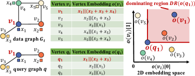
Figure 4. An example of vertex dominance embeddings in subgraph matching ( $||$ is the concatenation operation of two vectors).

Example 0.

Figure 4 shows an example of our vertex dominance embedding for subgraph matching between a snapshot graph $G_{t}$ and a query graph $q$. Based on Eq. (3), we can obtain the embedding for each vertex in $G_{t}$ or $q$. For example, vertices $v_{1}$ and $q_{1}$ have the embeddings $o(v_{1})=x_{1}||(x_{2}+x_{3}+x_{4})$ and $o(q_{1})=x_{1}||(x_{2}+x_{3})$, respectively.

Since vertex $q_{1}$ in $q$ matches with vertex $v_{1}$ in (a subgraph of) $G_{t}$, we can see that $o(q_{1})$ is dominating $o(v_{1})$ in a 2D embedding space (based on the property of vertex dominance embedding), which implies that $g_{q_{1}}$ is potentially a subgraph of (i.e., matching with) $g_{v_{1}}$. Moreover, although $o(v_{2})$ is dominated by $o(q_{1})$, $g_{v_{2}}$ does not match $g_{q_{1}}$. Thus, in this case, vertex $v_{2}$ is a false positive during the subgraph candidate retrieval. On the other hand, since $o(q_{1})$ is not dominating $o(v_{3})$ in the 2D embedding space, query vertex $q_{1}$ cannot match with vertex $v_{3}$ in graph $G_{t}$.   $\blacksquare$

Ease of Incremental Updates for Vertex Dominance Embeddings: In the dynamic graph $G_{D}$, our proposed vertex dominance embedding $o(v_{i})$ can be incrementally maintained, upon graph update operations in $\Delta G_{t}$.

Specifically, any edge insertion $(e+,t)$ or deletion $(e-,t)$ (as given in Definition 2.4) will affect the embeddings of two ending vertices, $v_{i}$ and $v_{j}$, of edge $e=(v_{i},v_{j})$. We consider incremental update of the embedding vector $o(v_{i})$ for vertex $v_{i}$ as follows.

• When $v_{i}$ is a newly inserted vertex, we obtain its embedding vector $o(v_{i})$ from scratch (i.e., $o(v_{i})=x_{i}||x_{j}$), and;

• When $v_{i}$ is an existing vertex in dynamic graph $G_{D}$, for an insertion (or deletion) operator of edge $e=(v_{i},v_{j})$, we update the SPAN vector, $y_{i}$, in $o(v_{i})$ with $(y_{i}+x_{j})$ (or $(y_{i}-x_{j})$), where $x_{j}$ is the SPUR vector of vertex $v_{j}$.

The embedding update of vertex $v_{j}$ is similar and thus omitted.

Note that, for each graph update (i.e., edge insertion $(e+,t)$ or deletion $(e-,t)$), the time complexity of incrementally updating vertex dominance embedding vectors is given by $O(d)$, where $d$ is the dimension of SPUR/SPAN vectors.

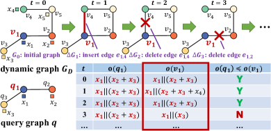
Figure 5. An example of vertex embeddings for DSM.

Example 0.

Figure 5 illustrates an example of using our vertex dominance embeddings to conduct the subgraph matching over dynamic graph $G_{D}$ over time $t$ from 0 to 3, where $q$ is a given query graph. Consider two vertices $v_{1}$ and $q_{1}$ in graphs $G_{D}$ and $q$, respectively. At timestamp $t=0$, their vertex embeddings satisfy the dominance relationship, that is, $o(q_{1})\preceq o(v_{1})$, thus, vertex $v_{1}$ is a candidate matching with $q_{1}$.

At timestamp $t=1$, a new edge $e_{1,4}$ is inserted (i.e., $\Delta G_{1}$), and the vertex embedding $o(v_{1})$ changes from $x_{1}||(x_{2}+x_{3})$ to $x_{1}||(x_{2}+x_{3}+x_{4})$ (by including new neighbor $v_{4}$’s SPUR vector $x_{4}$). Since $o(q_{1})\preceq o(v_{1})$ still holds, $v_{1}$ remains a candidate matching with $q_{1}$.

At timestamp $t=2$, since edge $e_{1,4}$ is deleted (i.e., $\Delta G_{2}$), the vertex embedding $o(v_{1})$ changes back to $x_{1}||(x_{2}+x_{3})$. At timestamp $t=3$, edge $e_{1,2}$ is deleted (i.e., $\Delta G_{3}$), and $o(v_{1})$ is updated with $x_{1}||(x_{3})$ (by removing the expired neighbor $v_{2}$’s SPUR vector $x_{2}$). In this case, $o(q_{1})\preceq o(v_{1})$ does not hold, and vertex $v_{1}$ fails to match with $q_{1}$. $\blacksquare$

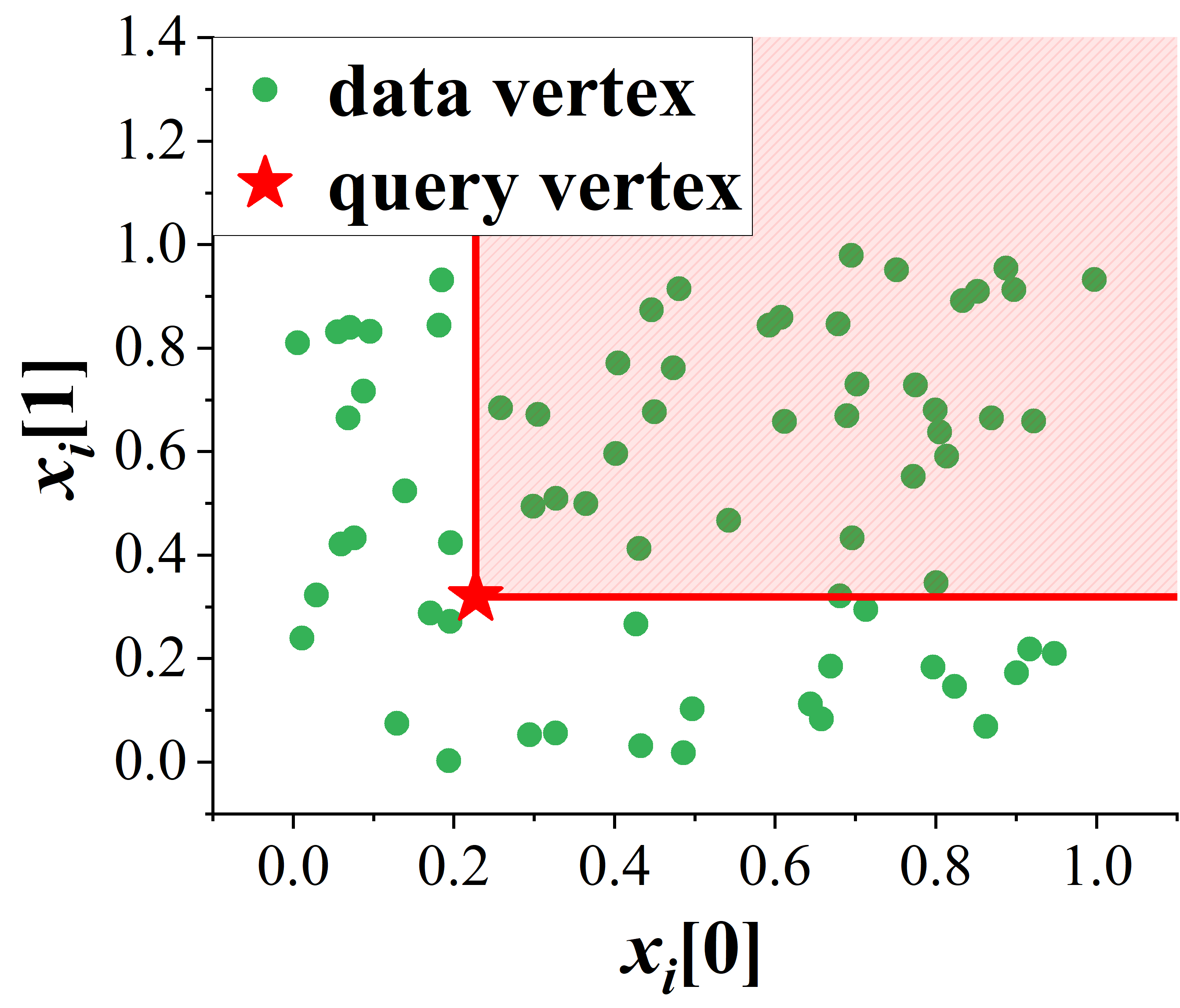
(a) SPUR vectors $x_{i}$

(b) SPAN vectors $y_{i}$

Figure 6. An example of SPUR/SPAN vector distributions in vertex dominance embedding $o(v_{i})$.

4.4. Embedding Optimization with Base Vector $z_{i}$

Figure 6 shows the distributions of 2D SPUR and SPAN vectors, $x_{i}$ and $y_{i}$, respectively, in vertex dominance embedding $o(v_{i})$ over Yeast graph (Sun and Luo, 2020) (with 3,112 vertices and 12,519 edges). We can see that, in Figure 6(a), the SPUR vectors $x_{i}$ generated by a seeded randomized function are distributed uniformly in the embedding space, whereas the SPAN vectors (i.e., the summed SPUR vectors) $y_{i}$ are more clustered along the reverse diagonal line in Figure 6(a).

As mentioned in Section 4.3, given a query vertex $q_{i}$, we can use its embedding vector $o(q_{i})$ as a query point to find the dominated embedding vectors $o(v_{i})$ ($=x_{i}\text{ }||\text{ }y_{i}$) in the 4D embedding space. Due to the scattered SPUR/SPAN vectors in the embedding space, it is very likely that some false alarms of embedding vectors $o(v_{i})$ are included as candidate matching vertices (i.e., dominated by $o(q_{i})$) .

In order to further enhance the pruning power, our goal is to update our vertex dominance embedding vector from $o(v_{i})$ to $o^{\prime}(v_{i})$, such that the number of candidate vertices dominated by $o(q_{i})$ is reduced (i.e., as small as possible). Specifically, we have the optimized embedding $o^{\prime}(v_{i})$, given by:

(4) $$o^{\prime}(v_{i})=\alpha(x_{i}||y_{i})+\beta z_{i},$$

where $\alpha$ and $\beta$ are positive constants ($\alpha\ll\beta$), and $z_{i}=f_{2}(l(v_{i}))$ is a random base vector of size $(2d)$, generated by a pseudo-random function $f_{2}(\cdot)$ with $l(v_{i})$ as the seed. Please refer to Figure 3 on how to compute this optimized vertex dominance embedding.

Note that, since the base vector $z_{i}$ is generated only based on the label $l(v_{i})$ of center vertex $v_{i}$, different star subgraphs with the same center vertex label $l(v_{i})$ will result in the same base vector $z_{i}$. Therefore, the new (optimized) vertex embedding vector $o^{\prime}(v_{i})$ in Eq. (4) still follows the dominance relationship, that is, $o^{\prime}(q_{i})\preceq o^{\prime}(v_{i})$ holds, if a query star pattern $s_{q_{i}}$ is a subgraph of unit star subgraph $g_{v_{i}}$ (i.e., $s_{q_{i}}\subseteq g_{v_{i}}$ and $l(q_{i})\equiv l(v_{i})$).

Lemma 4.4.

(The Dominance Property of the Optimized Vertex Embeddings) Given a unit star subgraph $g_{v_{i}}$ centered at vertex $v_{i}$ and any of its star substructures $s_{v_{i}}$ (i.e., $s_{v_{i}}\subseteq g_{v_{i}}$), their optimized vertex embeddings (via base vector $z_{i}$) satisfy the condition that: $o^{\prime}(s_{v_{i}})\preceq o^{\prime}(g_{v_{i}})$ (including $o^{\prime}(s_{v_{i}})=o^{\prime}(g_{v_{i}})$).

Proof.

Given a unit star subgraph $g_{v_{i}}$ centered at vertex $v_{i}$ and any of its star substructures $s_{v_{i}}$ (i.e., $s_{v_{i}}\subseteq g_{v_{i}}$), since they have the same center vertex $v_{i}$ (with the same vertex label), their base vectors have the same values, i.e., $z_{i}(s_{v_{i}})=z_{i}(g_{v_{i}})$, or equivalently $\beta z_{i}(s_{v_{i}})=\beta z_{i}(g_{v_{i}})$ (for $\beta>0$).

Due to the property of vertex dominance embeddings (as given in Lemma LABEL:lemma:embedding_property), we have $o(s_{v_{i}})\preceq o(g_{v_{i}})$, or equivalently $\alpha o(s_{v_{i}})\preceq\alpha o(g_{v_{i}})$ (for $\alpha>0$).

Therefore, we can derive that $\alpha o(s_{v_{i}})+\beta z_{i}(s_{v_{i}})\preceq\alpha o(g_{v_{i}})+\beta z_{i}(g_{v_{i}})$, or equivalently $o^{\prime}(s_{v_{i}})\preceq o^{\prime}(g_{v_{i}})$ (including $o^{\prime}(s_{v_{i}})=o^{\prime}(g_{v_{i}})$), which completes the proof. ∎

Discussions on How to Design a Base Vector, $z_{i}$: To improve the pruning power, we would like to make the distribution of the updated vertex embeddings in Eq. (4) more dispersed along diagonal line (or plane), so that fewer false alarms (dominated by $o^{\prime}(q_{i})$) can be obtained during dynamic subgraph matching.

In this paper, we propose to design the base vector $z_{i}$ as a random vector distributed on the unit diagonal line/hyperplane ($L_{1}$-norm) in the first quadrant. That is, we can normalize $z_{i}$ to $\frac{z_{i}}{||z_{i}||_{1}}$, where $||\cdot||_{1}$ is $L_{1}$-norm. Moreover, since constant $\alpha$ is far smaller than $\beta$, $\alpha(x_{i}||y_{i})$ can be considered as noises added to the scaled base vector $\beta z_{i}$. Thus, vertex embedding vectors $o^{\prime}(v_{i})$ ($=\alpha(x_{i}||y_{i})+\beta z_{i}$) in Eq. (4) are still distributed close to a diagonal line (or hyperplane) in the first quadrant.

We would like to leave interesting topics of using other base vectors $z_{i}$ (e.g., $L_{2}$-norm) as our future work.

Figure 7 shows the distributions of the updated 2D SPUR and SPAN vectors (from $o^{\prime}(v_{i})$), by adding a base vector $z_{i}$, where $z_{i}$ is given by $L_{1}$-norm. Since we have $\alpha\ll\beta$ in Eq. (4), after adding $\alpha(x_{i}||y_{i})$ to the scaled base vector $\beta z_{i}$, the previous embedding vector $o(v_{i})$ (as shown in Figure 6) is re-located close to diagonal lines in Figure 7. This way, we can reduce the number of vertex false alarms dominated by $o(q_{i})$ in both SPUR and SPAN spaces.

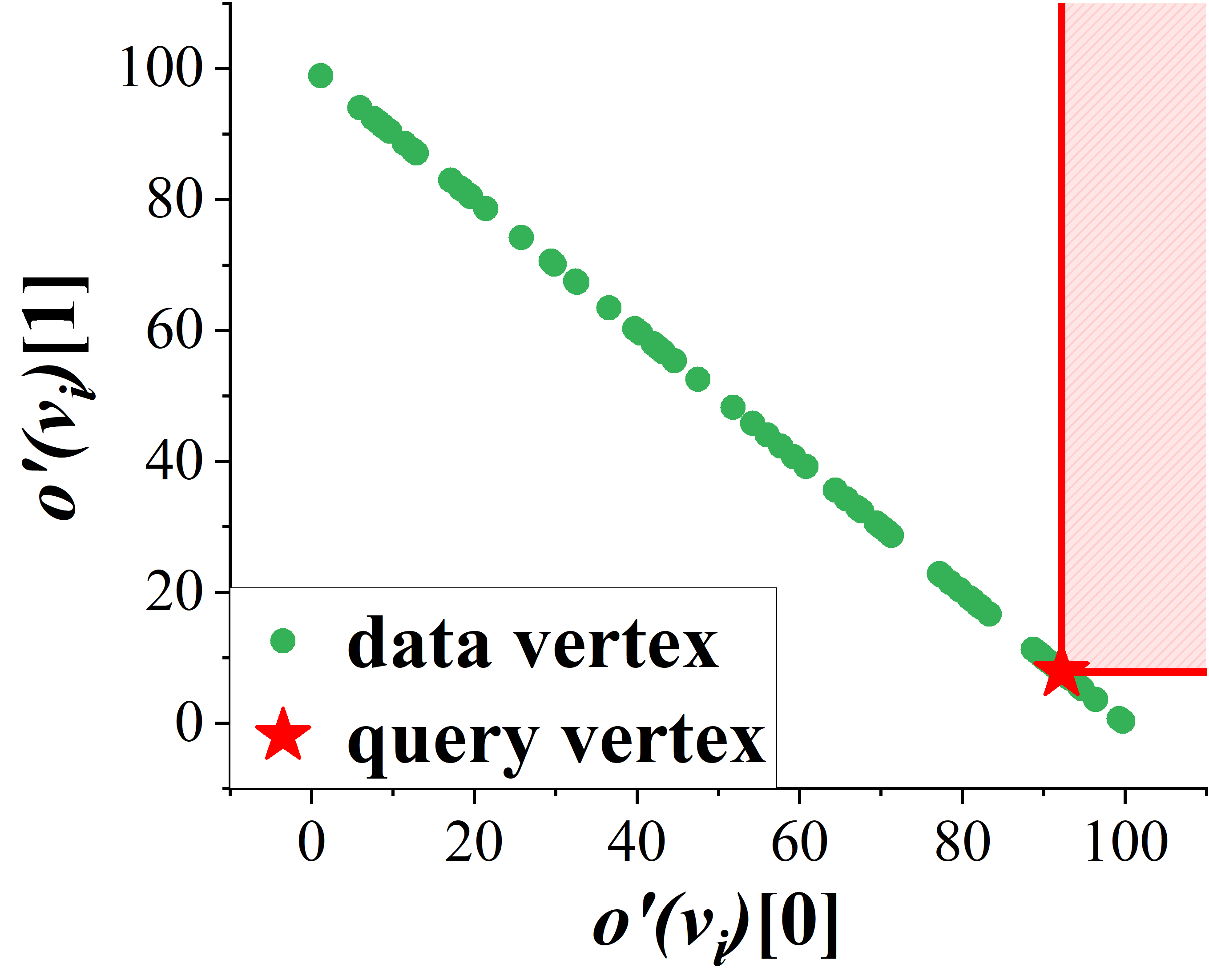
(a) $\alpha x_{i}+\beta(z_{i}[0],z_{i}[1])^{T}$

(b) $\alpha y_{i}+\beta(z_{i}[2],z_{i}[3])^{T}$

Figure 7. An example of $o^{\prime}(v_{i})$ distributions with $L_{1}$-norm diagonal-line base vector $z_{i}$ ($\alpha=0.01,\beta=100$).

5. Degree-Aware Star Substructure Synopses

In this section, we will build effective synopses over embeddings of star substructures of different degrees in dynamic graph $G_{D}$, which can be incrementally updated and support efficient DSM query processing.

5.1. Vertex Embedding via Degree Grouping

Note that, for the subgraph matching over a dynamic graph $G_{t}$, those vertices $v_{i}\in V(G_{t})$ with high degrees $deg(v_{i})$ are less likely to be pruned in the embedding space. This is because, for high degrees, the SPAN vectors in $o^{\prime}(v_{i})$ tend to have large values. Thus, $o^{\prime}(v_{i})$ is more likely to be dominated by query embedding vector $o^{\prime}(q_{i})$, and treated as candidate vertices for the refinement (i.e., $v_{i}$ cannot be pruned).

To enhance the pruning power for high-degree vertices, in this subsection, we propose a novel and effective degree grouping technique, which separately maintains vertex embeddings, $o^{\prime}(v_{i})$, for star substructures $s_{v_{i}}$ of different (lower) degree groups (instead of unit star subgraph $g_{v_{i}}$) in $G_{t}$.

Equi-Frequency Degree Grouping: One straightforward way to perform the degree grouping is to let each single degree value be a degree group. However, since vertex degrees in real-world graphs usually follow the power-law distribution (Barabási and Albert, 1999; Newman, 2005; Barabási and Bonabeau, 2003; Albert and Barabási, 2002; Dorogovtsev and Mendes, 2003), only a small fraction of vertices have high degrees. In other words, only a few unit star subgraphs $g_{v_{i}}$ have star substructures $s_{v_{i}}$ of very high degrees, which is not space- and time-efficient to maintain in a dynamic graph $G_{t}$.

Inspired by this, in this paper, we propose to maintain vertex embeddings for star substructures with $m$ degree groups (of different degree intervals). We assume that the degree statistics of the initial graph $G_{0}$ are similar to that in $G_{t}$.

This way, we obtain the probability mass function of vertex degrees in $G_{0}$ is $pmf(\delta)=\frac{freq(deg(v_{i})\geq\delta)}{|V(G_{0})|}$, where $freq(deg(v_{i})\geq\delta)$ is the number of vertices $v_{i}\in V(G_{0})$ whose degrees are greater than or equal to a degree value $\delta$. Our goal is to divide the degree interval, $[1,deg_{max}]$, into $m$ degree groups $\mathcal{B}=\{B_{1},B_{2},\cdots,B_{m}\}$, such that each degree bucket $B_{j}$ ($=(\delta_{j-1},\delta_{j}]$) contains the same (or similar) mass in the distribution of $pmf(\delta)$ (for $\delta\in B_{j}$).

5.2. The Construction of Degree-Aware Star Substructure Synopses (DAS³)

Based on the degree grouping, we will construct $m$ degree-aware star substructure synopses (DAS³), $Syn_{j}$ (for $1\leq j\leq m$), which are essentially $m$ grid files (Güting, 1994), respectively, that store (aggregated) vertex embeddings for star substructures in specific degree groups.

Data Structure of DAS³ Synopses: Specifically, each DAS³ synopsis $Syn_{j}$ partitions the embedding data space into cells, $C$, of equal size. Each grid cell $C$ is associated with a list, $C.list$, of vertices $v_{i}$. Each vertex $v_{i}\in C.list$ contains the following aggregates:

• an embedding upper bound vector, $v_{i}.UB_{\delta}$, for all star substructures $s_{v_{i}}$ with center vertex degrees $\delta\in(\delta_{j-1},\delta_{j}]$, and;

• a list of MBRs, $v_{i}.MBR_{\delta}$ (for $\delta\in(\delta_{j-1},\delta_{j}]$), that minimally bound all embedding vectors, $o^{\prime}(s_{v_{i}})$, of star substructures $s_{v_{i}}$ with degrees equal to $\delta$.

To facilitate the access of cells in DAS³ synopsis $Syn_{j}$ efficiently, we sort all cells in descending order of their keys $C.key$. Here, for each cell $C$, we use $C.UB$ to denote its maximal corner point (i.e., taking the maximum value of the cell interval on each dimension). The key, $C.key$, is defined as $||C.UB||_{2}$, where $||Z||_{2}=\sum_{i=1}^{d}Z[i]^{2}$ for a $d$-dimensional vector $Z$.

Note that, if a query vertex embedding $o(q_{i})$ dominates $C.UB$, then the key $||o(q_{i})||_{2}$ of query vertex embedding $o(q_{i})$ must be smaller than or equal to the cell key $C.key$. Thus, with such a sorted list of cells, we can efficiently access all cells that are fully or partially dominated by a given query vertex embedding $o(q_{i})$.

DAS³ Synopsis Construction: Each DAS³ synopsis $Syn_{j}$ corresponds to a degree group $B_{j}$ ($1\leq j\leq m$) with degree interval $(\delta_{j-1},\delta_{j}]$. We build the DAS³ synopsis $Syn_{j}$ as follows. For each vertex $v_{i}$ with degree $deg(v_{i})>\delta_{j-1}$ in $G_{t}$ and for each degree value $\delta$ ($\in(\delta_{j-1},\delta_{j}]$), we obtain all its star substructures, $s_{v_{i}}$, with degrees of center vertex $v_{i}$ equal to $\delta$, compute their embedding vectors $o^{\prime}(s_{v_{i}})$, and use a minimum bounding rectangle (MBR), $v_{i}.MBR_{\delta}$, to minimally bound these embedding vectors.

Let $v_{i}.UB_{\delta}$ be the maximum corner point of the MBR $v_{i}.MBR_{\delta}$ (by taking the upper bound of the MBR on each dimension). Then, for vertex $v_{i}$, we insert vertex $v_{i}$ into the vertex list, $C.list$, of a cell $C\in\mathcal{I}_{j}$, into which corner point $v_{i}.UB_{ub\_\delta}$ falls, where degree upper bound $ub\_\delta=\min\{deg(v_{i}),\delta_{j}\}$. Intuitively, this corner point $v_{i}.UB_{ub\_\delta}$ is the one most likely to be dominated by a query vertex embedding $o^{\prime}(q_{i})$ in this degree group $B_{j}$.

Moreover, we also associate corner point $v_{i}.UB_{ub\_\delta}$ with the list of MBRs, $v_{i}.MBR_{\delta}$ (for each $\delta\in(\delta_{j-1},ub\_\delta]$), in synopsis $Syn_{j}$, which can be used for further pruning for a specific degree in interval $(\delta_{j-1},\delta_{j}]$.

Discussions on MBR Computations and Incremental Maintenance: Note that, the MBRs, $v_{i}.MBR_{\delta}$, mentioned above minimally bound embedding vectors $o^{\prime}(v_{i})$ for all star substructures $s_{v_{i}}$. Since there are an exponential number of possible star structures (i.e., $2^{deg(v_{i})}$), it is not efficient to enumerate all star substructures, compute their embedding vectors, and obtain the MBRs. Therefore, in this paper, we propose a sorting-based method to obtain $v_{i}.MBR_{\delta}$ without enumerating all star substructures with degree $\delta$.

Specifically, for each vertex $v_{i}$, we maintain $d$ sorted lists, each of which, $v_{i}.spur\_list_{k}$ (for $1\leq k\leq d$), contains the $k$-th elements, $y_{j}[k]$, of SPUR vectors $y_{j}$ (obtained from $v_{i}$’s 1-hop neighbors $v_{j}\in\mathcal{N}(v_{i})$) in ascending order.

For a degree $\delta$ in the degree group $B_{j}=(\delta_{j-1},\delta_{j}]$, we obtain lower and upper bounds of MBR $v_{i}.MBR_{\delta}$, that is, $v_{i}.MBR_{\delta}[2k]$ and $v_{i}.MBR_{\delta}[2k+1]$, respectively, as follows:

(5) $$v_{i}.MBR_{\delta}[2k] = \sum_{deg\in[1,\delta]}v_{i}.spur\_list_{k}[deg],$$

(6) $$v_{i}.MBR_{\delta}[2k+1] = \sum_{deg\in[deg(v_{i})-\delta+1,deg(v_{i})]}v_{i}.spur\_list_{k}[deg],$$

where $deg(v_{i})$ is the degree of vertex $v_{i}$ in $G_{t}$ (or the size of the sorted list $v_{i}.spur\_list_{k}$).

Intuitively, Eqs. (5) and (6) give the lower/upper bounds of the MBR $v_{i}.MBR_{\delta}$ on the $k$-th dimension, by summing up the first $\delta$ and the last $\delta$ values, respectively, in the sorted list $v_{i}.spur\_list_{k}$.

The Time Complexity of the MBR Maintenance: The time complexity of sorting the $k$-th dimension of SPUR vectors (for $1\leq k\leq d$) is given by $O(d\cdot deg(v_{i})\cdot log(deg(v_{i})))$, which is much less than that of enumerating all star substructures (i.e., $O(d\cdot 2^{deg(v_{i})})$).

For the maintenance of a sorted list $v_{i}.spur\_list_{k}$ in dynamic graph $G_{t}$, upon edge insertion or deletion (or insertion/deletion of a 1-hop neighbor $v_{j}$), we can use a binary search to locate where we need to insert into (or remove from) $v_{i}.spur\_list_{k}$ elements $y_{j}[k]$ in the SPUR vector $y_{j}$. Therefore, the time complexity of incrementally maintaining $d$ sorted lists $v_{i}.spur\_list_{k}$ is given by $O(d\cdot log_{2}(deg(v_{i})))$.

6. DSM Query Processing

In this section, we will illustrate query processing algorithms based on vertex dominance embeddings in DAS³ synopses to efficiently answer DSM queries.

6.1. Synopsis Pruning Strategies

Given a query vertex $q_{i}$ in the query graph $q$ and SAS³ synopses $Syn_{j}$, we would like to obtain candidate vertices $v_{i}$ from synopsis $Syn_{j}$ which may match with the query vertex $q_{i}$, where $deg(q_{i})$ falls into the degree group $B_{j}=(\delta_{j-1},\delta_{j}]$.

In this subsection, we present two effective pruning methods over index $Syn_{j}$, named embedding dominance pruning and MBR range pruning, which are used to rule out false alarms of cells/vertices.

Embedding Dominance Pruning: We first provide the embedding dominance pruning method, which filters out those cells/vertices in synopsis $Syn_{j}$ that are not dominated by a given query embedding vector $o^{\prime}(q_{i})$.

Lemma 6.1.

(Embedding Dominance Pruning) Given a query embedding vector $o^{\prime}(q_{i})$ of the query vertex $q_{i}$, any cell $C$ or vertex $v_{i}$ can be safely pruned, if $o^{\prime}(q_{i})$ does not dominate any portion of cell $C$ or embedding upper bound vector $v_{i}.UB_{\delta}$.

Proof.

If a query vertex $q_{i}$ in query graph $q$ matches with a data vertex $v_{i}$ in a subgraph of the data graph, then their vertex dominance embeddings must hold that $o^{\prime}(q_{i})\preceq o^{\prime}(v_{i})$. Therefore, if $o^{\prime}(q_{i})$ does not dominate the cell $C$, then $o^{\prime}(q_{i})$ cannot dominate any vertex $o^{\prime}(v_{i})$ inside cell $C$, and all vertices in cell $C$ (or cell $C$) can be safely pruned.

Moreover, if $o^{\prime}(q_{i})$ does not dominate embedding upper bound vector $v_{i}.UB_{\delta}$, i.e., $v_{i}.UB_{\delta}\notin DR(o^{\prime}(q_{i}))$, then $o^{\prime}(q_{i})$ does not dominate any star substructure $s_{v_{i}}$ with center vertex $v_{i}$ and the corresponding degree group. In other words, $q_{i}$ does not match with $v_{i}$. Thus, vertex $v_{i}$ can be safely pruned. ∎

MBR Range Pruning: Next, we give an effective MBR range pruning method, which further utilizes the MBR ranges, $v_{i}.MBR_{\delta}$, of star substructure embeddings and prunes vertices $v_{i}$ that do not fall into the MBRs.

Lemma 6.2.

(MBR Range Pruning) Given a query embedding $o^{\prime}(q_{i})$ of the query vertex $q_{i}$ and a vertex $v_{i}$ in a cell of DAS³ synopsis $Syn_{j}$ (for $deg(q_{i})\in(\delta_{j-1},\delta_{j}]$), vertex $v_{i}$ can be safely pruned, if it holds that $o^{\prime}(q_{i})\notin v_{i}.MBR_{deg(q_{i})}$.

Proof.

The MBR $v_{i}.MBR_{deg(q_{i})}$ minimally bounds vertex embeddings for all possible star substructures $s_{v_{i}}$ with center vertex $v_{i}$ and degree $deg(q_{i})$. Thus, if query vertex $q_{i}\in V(q)$ and its 1-hop neighbors match with some star substructures with the same degree $deg(q_{i})$, then its query embedding vector $o^{\prime}(q_{i})$ must fall into this MBR $v_{i}.MBR_{deg(q_{i})}$. Therefore, if this condition does not hold, i.e., $o^{\prime}(q_{i})\notin v_{i}.MBR_{deg(q_{i})}$, then $q_{i}$ does not match with $v_{i}$, and $v_{i}$ can be safely pruned, which completes the proof. ∎

Input: i) a snapshot graph $G_{t}$ at current timestamp $t$; ii) a DAS³ synopsis $Syn_{j}$ on $G_{t}$, and; iii) a query graph $q$

Output: a set, $A(q,t)$, of initial subgraph matching results in $G_{t}$

1

2compute vertex dominance embeddings $o^{\prime}(q_{i})$ for all query vertices $q_{i}\in V(q)$

// traverse synopses $Syn_{j}$ to obtain candidate vertices

3 for each query vertex $q_{i}\in V(q)$ do

4       obtain a synopsis $Syn_{j}$ such that $deg(q_{i})\in(\delta_{j-1},\delta_{j}]$

5       for each cell $C\in Syn_{j}$ with $C.key\geq||o^{\prime}(q_{i})||_{2}$ do

6             for each candidate vertex $v_{i}\in C.list$ do

7                   if $o^{\prime}(q_{i})\preceq v_{i}.UB_{\delta}$  then

8                         if $o^{\prime}(q_{i})\in v_{i}.MBR_{deg(q_{i})}$  then

                               $q_{i}.cand\_set\leftarrow q_{i}.cand\_set\cup\{v_{i}\}$  // Lemmas 6.1 and  6.2

9                              

10                        

11                  

12            

13      

// generate a query plan $Q$

14

15select a query vertex $q_{i}$ with the smallest candidate set size $|q_{i}.cand\_set|$ as the first query vertex in an ordered list $Q$

16

17iteratively select a neighbor $q_{k}$ of $q_{i}\in Q$ with minimum $|q_{k}.cand\_set|$ and append $q_{k}$ to $Q$, until all query vertices in $V(q)$ have been added to $Q$

18

// assemble and refine candidate subgraphs

19 $A(q,t)\leftarrow\emptyset$

20 invoke Refinement$(q,Q,G_{t},A(q,t),\emptyset,0)$ to obtain actual DSM query answers in $A(q,t)$

21 return $A(q,t)$;

Algorithm 2 Initial DSM Answer Set Generation

6.2. Initial DSM Answer Set Generation

Algorithm 2 illustrates the algorithm of generating the initial subgraph matching answer set, $A(q,t)$, over a snapshot $G_{t}$ of a dynamic subgraph $G_{D}$, by traversing synopses over vertex dominance embeddings. Specifically, given a query graph $q$, we first obtain vertex dominance embeddings $o^{\prime}(q_{i})$ for each query vertex $q_{i}\in V(q)$ (line 1), and then traverse DAS³ synopses, $Syn_{j}$, to retrieve vertex candidate sets $q_{i}.cand\_set$ (lines 2-8). Next, we generate a query plan $Q$, which is an ordered list of connected query vertices that can be used to join their corresponding candidate vertices (lines 9-10). Finally, we assemble candidate vertices into candidate subgraphs, and refine candidate subgraphs by the left-deep join based method (Kankanamge et al., 2017; Shang et al., 2008) by invoking function Refinement($\cdot$), and return the initial subgraph matching answers in $A(q,t)$ (lines 11-13).

The Synopsis Search: For each query vertex $q_{i}\in V(q)$, we first need to find a synopsis $Syn_{j}$ that matches the degree group of $q_{i}$ (i.e., $deg(q_{i})\in(\delta_{j-1},\delta_{j}]$ must hold; line 3).

As mentioned in Section 5.2, cells, $C$, in the DAS³ synopsis $Syn_{j}$ are sorted in descending order of their keys $C.key$. We thus only need to search for those cells $C\in Syn_{j}$ satisfying the condition that $C.key\geq||o^{\prime}(q_{i})||_{2}$ (line 4). Then, for each candidate vertex $v_{i}\in C.list$, we apply our proposed embedding dominance and MBR range pruning strategies (as discussed in Lemmas 6.1 and 6.2, respectively), and obtain the candidate vertex set, $q_{i}.cand\_set$, for the query vertex $q_{i}$ (lines 5-8).

Query Plan Generation: After obtaining candidate vertices, we generate a query plan $Q$ for refinement. Intuitively, we would like to reduce the size of intermediate join results. Therefore, we first initialize $Q$ with a query vertex $q_{i}\in V(q)$ having the minimum candidate set size $|q_{i}.cand\_set|$ (line 9), and then iteratively add to $Q$ the one, $q_{k}$, that is connected with those selected query vertices in $Q$ and having the smallest $|q_{k}.cand\_set|$ value (line 10).

Input: i) a query graph $q$; ii) a sorted list (query plan) $Q$; iii) a snapshot graph $G_{t}$; iv) matching results set $A$; v) a sorted list, $M$, of vertices matching with query vertices in $Q$, and; vi) the recursion depth $n$

Output: a set, $A$, of subgraph matching results

1

2if $n=|Q|$ then

3       $A\leftarrow A\cup\{M\}$

4       return;

5      

6else

7       $S_{cand}=\emptyset$

8       if $n=0$ then

9             $S_{cand}\leftarrow S_{cand}\cup Q[n].cand\_set$

10            

11      else

12             for each candidate vertex $u\in Q[n].cand\_set$ and $u\notin M$ do

13                   if edges $(M[i],u)$ exist in $E(G_{t})$ for all edges $(Q[i],Q[n])\in E(q)$ (for $0\leq i<n$) then

14                         $S_{cand}\leftarrow S_{cand}\cup\{u\}$

15                        

16                  

17            

18      

19for each candidate vertex $u\in S_{cand}$ do

20       $M[n]=u$

21       Refinement ($q,Q,G_{t},A,M,n+1$);

22      

Algorithm 3 Refinement

Refinement: Algorithm 3 uses a left-deep join based method (Kankanamge et al., 2017; Shang et al., 2008) to assemble candidate vertices in $q_{i}.cand\_set$ into candidate subgraphs, and obtain the actual matching subgraph answer set $A(q,t)$ (i.e., lines 11-13 of Algorithm 2).

Specifically, we maintain a vertex vector $M$ that will store vertices of the subgraph $g$ matching with ordered query vertices in $Q$. To enumerate all matching subgraphs, each time we recursively expand partial matching results by including a new candidate vertex $u$ as $M[n]$ that maps with the $n$-th query vertex $Q[n]$. If we find all vertices in $M$ mapping with $Q$ (i.e., recursion depth $n=|Q|$), then we can add $M$ to the answer set $A$ (lines 1-3). Otherwise, we will find a vertex candidate set $S_{cand}$ from $Q[n].cand\_set$, such that each vertex $u$ in $S_{cand}$ has the same edge connections to that in $M$ as that in $Q$ (lines 5-11). Next, for each vertex $u\in S_{cand}$, we treat it as vertex $M[n]$ matching with $Q[n]$, and recursively call function Refinement($\cdot$) with more depth $n+1$ (lines 13-17).

After the recursive function Refinement($\cdot$) has been executed, the answer set $A$ (or $A(q,t)$ in Algorithm 3) will contain a set of actual subgraph matching results.

Complexity Analysis: In Algorithm 2, since we need to access each query vertex $q_{i}$ and its 1-hop neighbors $\mathcal{N}_{v_{i}}$, the time complexity of computing vertex dominance embeddings $o^{\prime}(q_{i})$ (line 1) is given by $O(|V(q)|+|E(q)|)$.

For the synopsis traversal (lines 2-8), assume that $PP_{C}$ is the pruning power of the cells’ key value and $PP_{v}$ is the pruning power in each cell’s point list. Thus, the synopsis traversal cost is $O(|V(q)|\cdot(1-PP_{C})K^{d}\cdot(1-PP_{v})|C.list|)$, where $K^{d}$ is the number of cells and $|C.list|$ is the number of vertices in the cell $C$.

Next, for the greedy-based query plan generation (lines 9-10), we need to iteratively select a neighbor of vertices in the query plan $Q$, which requires $O(|V(q)|^{2})$ cost.

Finally, we invoke the recursive function Refinement($\cdot$) to find actual subgraph matching results (lines 11-13), with the worst-case time complexity $O(\prod_{i=0}^{|V(q)|-1}|q_{i}.cand\_set|)$.

Therefore, the overall time complexity of Algorithm 2 is given by: $O(|V(q)|+|E(q)|+|V(q)|\cdot(1-PP_{C})K^{d}\cdot(1-PP_{v})|C.list|+\prod_{i=0}^{|V(q)|-1}|q_{i}.cand\_set|+|V(q)|^{2})$.

6.3. DSM Query Answering

Given a dynamic graph $G_{t-1}$ at timestamp $(t-1)$, a registered query graph $q$, and a graph update operation $\Delta G_{t}$ at timestamp $t$, Algorithm 4 provides a DSM query answering algorithm, which maintains/obtains the latest subgraph matching answer set, $A(q,t)$.

Specifically, if the graph update operation $\Delta G_{t}$ is an insertion of edge $e=(v_{i},v_{j})$, we will calculate an incremental update, $\Delta A(q,t)$, of new subgraph matching results (lines 1-11).

Edge Insertion: For the insertion of an edge $e=(v_{i},v_{j})$, we will first find matching edge(s) $(q_{i},q_{j})$ in the query graph with the same labels (line 3). Then, we will check whether or not edges $(v_{i},v_{j})$ and $(q_{i},q_{j})$ match each other, by applying the embedding dominance and MBR range pruning strategies (described in Section 6.1; lines 4-5). If the answer is yes, then we will generate a new query plan $Q^{\prime}$ starting from query vertices $q_{i}$ and $q_{j}$ (note: the remaining ones are obtained from $Q$, similar to line 10 of Algorithm 2; line 7), initialize the first two matching vertices $v_{i}$ and $v_{j}$ in a sorted list $M^{\prime}$ (lines 8-9), and invoke the function Refinement($\cdot$) with parameters of new query plan $Q^{\prime}$, incremental answer set $\Delta A(q,t)$, the initialized sorted list $M^{\prime}$, and recursion depth $n=2$ (as two matching vertices have been found; line 10). After that, we can update the answer set $A(q,t)$ with $A(q,t-1)\cup\Delta A(q,t)$ (line 11).

Edge Deletion: When $\Delta G_{t}$ is an edge deletion operation $(e-,t)$, we can simply remove those existing subgraph matching answers $g\in A(q,t-1)$ which contain the deleted edge $e$, and obtain the updated answer set $A(q,t)$ (lines 12-16).

Finally, we return the latest DSM query answer set $A(q,t)$ at timestamp $t$ (line 17).

Complexity Analysis: In Algorithm 4, for the edge insertion operation, we check all query edges, generate a new query plan $Q^{\prime}$, and refine new candidate subgraphs with the new edge (lines 1-11). Therefore, the worst-case time complexity is given by $O((|V(q)|^{2}+\prod_{i=2}^{|V(q)|-1}|Q^{\prime}[i].cand\_set|)\cdot|E(q)|)$.

For the edge deletion operation (lines 12-16), since we delete matching results from $A(q,t-1)$ that contain the deleted edge, by using the hash file to check the edge existence with $O(1)$ cost, the time complexity is given by $O(|A(q,t-1)|)$.

Input: i) a dynamic graph $G_{t-1}$ at previous timestamp $(t-1)$; ii) a graph update operation $\Delta G_{t}$; iii) a registered query graph $q$, and; iv) matching result set $A(q,t-1)$ at timestamp $(t-1)$

Output: an updated set, $A(q,t)$, of subgraph matching results at timestamp $t$

1

// edge insertion operation $\Delta G_{t}=(e+,t)$

2 if $\Delta G_{t}=(e+,t)$ for edge $e=(v_{i},v_{j})$ then

3       $\Delta A(q,t)\leftarrow\emptyset$

4       for each query edge $(q_{i},q_{j})\in E(q)$ with labels matching with that of $(v_{i},v_{j})$ do

             // check whether $(v_{i},v_{j})$ matches $(q_{i},q_{j})$

5             if $o^{\prime}(q_{i})\leq o^{\prime}(v_{i})$ and $o^{\prime}(q_{j})\leq o^{\prime}(v_{j})$ then

6                   if $o^{\prime}(q_{i})\in v_{i}.MBR_{deg(q_{i})}$ and $o^{\prime}(q_{j})\in v_{j}.MBR_{deg(q_{j})}$ then

                          // Lemmas 6.1 and  6.2

7                         generate a query plan $Q^{\prime}$ by using $q_{i}$ and $q_{j}$ as the first two query vertices and the remaining ones from $Q$

8                         $M^{\prime}[0]=v_{i}$

9                         $M^{\prime}[1]=v_{j}$

10                         invoke Refinement$(q,Q^{\prime},G_{t},\Delta A(q,t),M^{\prime},2)$ to incrementally obtain new matching results in $\Delta A(q,t)$

11                        

12                  

13            

14      $A(q,t)\leftarrow A(q,t-1)\cup\Delta A(q,t)$

15      

16else

      // edge deletion operation $\Delta G_{t}=(e-,t)$ for edge $e=(v_{i},v_{j})$

17       $A(q,t)=A(q,t-1)$

18       for each subgraph answer $g\in A(q,t-1)$ do

19             if edge $(v_{i},v_{j})$ exists in $E(g)$ then

20                   $A(q,t)\leftarrow A(q,t)-\{g\}$

21                  

22            

23      

24return $A(q,t)$

Algorithm 4 The Query Answering Algorithm for Continuous Dynamic Subgraph Matching Query

7. Cost-Model-Guided Embedding Optimization

In this section, we will design a novel cost model for evaluating the pruning power of our proposed vertex dominance embedding technique. Then, we will utilize this cost model to guide the embeddings and achieve better performance of dynamic subgraph matching.

7.1. Cost Model for Dynamic Subgraph Matching via Vertex Embeddings

In this subsection, we will propose a cost model to evaluate the performance of our dynamic subgraph matching (or the pruning power of using vertex dominance embeddings).

Specifically, we estimate the number, $Cost_{DSM}$, of candidate vertices $v_{i}$ (to retrieve and refine) whose embedding vectors $o^{\prime}(v_{i})$ are dominated by query embedding vector $o^{\prime}(q_{i})$ (given by Lemma 6.1). That is, we have:

(7) $$Cost_{DSM}=\sum_{v_{i}\in V(G_{t})}\prod_{j=1}^{2d}Pr\{o^{\prime}(q_{i})[j]\leq o^{\prime}(v_{i})[j]\},$$

where $2d$ is the dimension of the embedding vector $o^{\prime}(\cdot)$, and $Pr\{\cdot\}$ is a probability function.

Analysis of the Cost Model: We consider $o^{\prime}(v_{i})[j]$ as a random number generated from a random variable, with mean $\mu_{o^{\prime}(v_{i})[j]}$ and variance $\sigma_{o^{\prime}(v_{i})[j]}^{2}$. Moreover, $o^{\prime}(q_{i})[j]$ can be considered as a constant. We have the following equation:

(8) $$Pr\{o^{\prime}(q_{i})[j]\leq o^{\prime}(v_{i})[j]\}$$

$$= Pr\left\{\frac{(o^{\prime}(q_{i})[j]-o^{\prime}(v_{i})[j])-(o^{\prime}(q_{i})[j]-\mu_{o^{\prime}(v_{i})[j]})}{\sigma_{o^{\prime}(v_{i})[j]}^{2}}\right.$$

$$\left.\leq\frac{-(o^{\prime}(q_{i})[j]-\mu_{o^{\prime}(v_{i})[j]})}{\sigma_{o^{\prime}(v_{i})[j]}^{2}}\right\}.$$

By applying Central Limit Theorem (CLT) (Wikipedia, 2023) to Eq. (8), we have:

(9) $$Pr\{o^{\prime}(q_{i})[j]\leq o^{\prime}(v_{i})[j]\}\approx\Phi\left(\frac{\mu_{o^{\prime}(v_{i})[j]}-o^{\prime}(q_{i})[j]}{\sigma_{o^{\prime}(v_{i})[j]}^{2}}\right),$$

where $\Phi(\cdot)$ is the cumulative density function (cdf) of standard normal distribution.

We substitute Eq. (9) into Eq. (7) and obtain:

(10) $$Cost_{DSM}=|V(G_{t})|\cdot\prod_{j=1}^{2d}\Phi\left(\frac{\mu_{o^{\prime}(v_{i})[j]}-o^{\prime}(q_{i})[j]}{\sigma_{o^{\prime}(v_{i})[j]}^{2}}\right).$$

7.2. Design of Cost-Model-Based Vertex Dominance Embeddings

Eq. (10) estimates the (worst-case) query cost for one query vertex $q_{i}$ during the dynamic subgraph matching. Intuitively, our goal is to design vertex embeddings $o^{\prime}(\cdot)$ that minimizes the cost model $Cost_{DSM}$ (given in Eq. (10)).

Note that, $\Phi(\cdot)$ in Eq. (10) is a monotonically increasing function. Therefore, if we can minimize the term $\frac{\mu_{o^{\prime}(v_{i})[j]}-o^{\prime}(q_{i})[j]}{\sigma_{o^{\prime}(v_{i})[j]}^{2}}$ in Eq. (10), then low query cost $Cost_{DSM}$ can be achieved. In other words, guided by our proposed cost model (to minimize the query cost $Cost_{DSM}$), our target is to design/select a “good” distribution of vertex dominance embeddings $o^{\prime}(v_{i})$ with:

1. low mean $\mu_{o^{\prime}(v_{i})[j]}$ , and;

2. high variance $\sigma_{o^{\prime}(v_{i})[j]}^{2}$.

In this paper, unlike standard vertex dominance embeddings generated by Uniform random function $f_{1}(\cdot)$ (as discussed in Section 4.2), we choose to use a (seeded) Zipf random function to produce SPUR vectors $x_{i}$ in vertex embeddings $o^{\prime}(v_{i})$ (or in turn generate SPAN vectors $y_{i}=\sum x_{j}$). The $Zipf$ distribution exactly follows our target of finding a random variable with low mean and high variance, which can achieve low query cost, as guided by our proposed cost model $Cost_{DSM}$ (given in Eq. (7)). We would like to leave the interesting topic of studying other low-mean/high-variance distributions as our future work.

Discussions on the Seeded Zipf Generator: We consider two distributions, $Uniform$ and $Zipf$, each of which is divided to $b$ buckets with the same area. This way, we create a 1-to-1 mapping between buckets in a Uniform distribution and that in a $Zipf$ distribution. Given a seeded pseudo-random number, $r$, from the Uniform distribution, we can first find the bucket this Uniform random number falls into, obtain its corresponding bucket in the $Zipf$ distribution, and compute its proportional location $r^{\prime}$ in the $Zipf$ bucket. As a result, $r^{\prime}$ is the random number that follows the $Zipf$ distribution.

Integration of the Cost-Model-Based Vertex Embeddings into our Dynamic Subgraph Matching Framework: In light of our cost model above, we design a novel cost-model-based vertex dominance embedding, denoted as $o^{\prime}_{C}(v_{i})$, for each vertex $v_{i}$, that is:

(11) $$o^{\prime}_{C}(v_{i})=\alpha(x^{\prime}_{i}||y^{\prime}_{i})+\beta z_{i},$$

where $x^{\prime}_{i}=f_{Z}(l(v_{i}))$ is the newly designed SPUR vector generated by a seeded $Zipf$ random generator $f_{Z}(\cdot)$, and $y_{i}^{\prime}=\sum_{\forall v_{j}\in\mathcal{N}_{v_{i}}}x_{j}^{\prime}$.

Note that, since the SPAN vector $y^{\prime}_{i}$ in Eq. (11) is given by $\sum_{\forall v_{j}\in\mathcal{N}_{v_{i}}}x_{j}^{\prime}$, its distribution still follows the property of low mean and high variance to achieve low query cost.

8. Experimental evaluation

8.1. Experimental Settings

To evaluate the performance of our DSM approach, we conduct experiments on a Ubuntu server equipped with an Intel Core i9-12900K CPU and 128GB memory. Our source code in C++ and real/synthetic graph data sets are available at URL: https://github.com/JamesWhiteSnow/DSM.

Real/Synthetic Graph Data Sets: We evaluate our DSM approach over both real and synthetic graphs.

Real-world graphs. We test five real-world graph data used by previous works (He and Singh, 2008; Shang et al., 2008; Zhao and Han, 2010; Lee et al., 2012; Sun et al., 2012; Han et al., 2013; Ren and Wang, 2015; Bi et al., 2016; Katsarou et al., 2017; Bhattarai et al., 2019; Han et al., 2019; Sun and Luo, 2020), which can be classified into three categories: i) biology networks (Yeast and HPRD); ii) bibliographical/social networks (DBLP and Youtube), and; iii) citation networks (US Patents). Statistics of these real graphs are summarized in Table 2.

Table 2. Statistics of real-world graph data sets.

Data Sets	$|V(G)|$	$|E(G)|$	$|\sum|$	$avg\_deg(G)$
Yeast (ye)	3,112	12,519	71	8.0
HPRD (hp)	9,460	34,998	307	7.4
DBLP (db)	317,080	1,049,866	15	6.6
Youtube (yt)	1,134,890	2,987,624	25	5.3
US Patents (up)	3,774,768	16,518,947	20	8.8

Table 3. Parameter settings.

Parameters	Values
the dimension, $d$, of the SPUR/SPAN vector	1 2, 3, 4
the ratio, $\beta/\alpha$	10, 100, 1,000, 10,000, 100,000
the number, $m$, of degree groups	1, 2, 3, 4, 5
the number, $K$, of cell intervals in each dimension of $Syn_{j}$	1, 2, 5, 8, 10
the number, $|\Sigma|$, of distinct labels	5, 10, 15, 20, 25
the average degree, $avg\_deg(q)$, of the query graph $q$	2, 3, 4
the size, $|V(q)|$, of the query graph $q$	5, 6, 8, 10, 12
the average degree, $avg\_deg(G_{D})$, of dynamic graph $G_{D}$	3, 4, 5, 6, 7
the size, $|V(G_{D})|$, of the dynamic data graph $G_{D}$	10K, 30K, 50K, 80K, 100K, 500K, 1M

Synthetic graphs. We generate synthetic graphs via NetworkX (Hagberg and Conway, 2020), and produce small-world graphs following the Newman-Watts-Strogatz model (Watts and Strogatz, 1998). Parameter settings of synthetic graphs are depicted in Table 3. For each vertex $v_{i}$, we generate its label $l(v_{i})$ by randomly picking up an integer within $[1,|\sum|]$, following the $Uniform$, $Gaussian$, or $Zipf$ distribution. Accordingly, we obtain 3 types of graphs, denoted as $Syn\text{-}Uni$, $Syn\text{-}Gau$, and $Syn\text{-}Zipf$, resp.

The insertion (or deletion) rate is defined as the ratio of the number of edge insertions (or deletions) to the total number of edges in the raw graph data. Following the literature (Choudhury et al., 2015; Kim et al., 2018; Min et al., 2021; Sun et al., 2022a), we set the insertion rate to 10% by default (i.e., the initial graph $G_{0}$ contains 90% edges, and the remaining 10% edges arrive as the insertion stream). Similarly, for the case of edge deletions, we set the default deletion rate to 10% (i.e., initial graph $G_{0}$ contains all edges, and deletion operations of 10% edges arrive in the stream).

Query Graphs: Similar to previous works (Sun et al., 2012; Han et al., 2013; Ren and Wang, 2015; Bi et al., 2016; Katsarou et al., 2017; Archibald et al., 2019; Bhattarai et al., 2019; Han et al., 2019; Sun et al., 2022a), for each graph $G_{D}$, we randomly extract/sample 100 connected subgraphs as query graphs, where parameters of query graphs $q$ (e.g., $|V(q)|$ and $avg\_deg(q)$) are depicted in Table 3.

Baseline Methods: We compare our DSM approaches (using the cost-model-based vertex dominance embeddings $o^{\prime}_{C}(v_{i})$, as discussed in Section 7) with five representative baseline methods of dynamic subgraph matching as follows:

1. Graphflow (GF) (Kankanamge et al., 2017) is a direct-incremental algorithm that enumerates updates of matching results without any auxiliary data structure.

2. SJ-Tree (SJ) (Choudhury et al., 2015) is an index-based incremental method that evaluates the join query with binary joins using the index.

3. TurboFlux (TF) (Kim et al., 2018) is an index-based incremental method that stores matches of paths in $q$ without materialization and evaluates the query with the vertex-at-a-time method.

4. SymBi (Sym) (Min et al., 2021) is an index-based incremental method that prunes candidate vertex sets using all query edges.

5. IEDyn (IED) (Idris et al., 2017, 2020) is an index-based incremental method that supports acyclic queries and can achieve constant delay enumeration under the setting of graph homomorphism.

We used the code of baseline methods from (Sun et al., 2022a), which is implemented in C++ for a fair comparison.

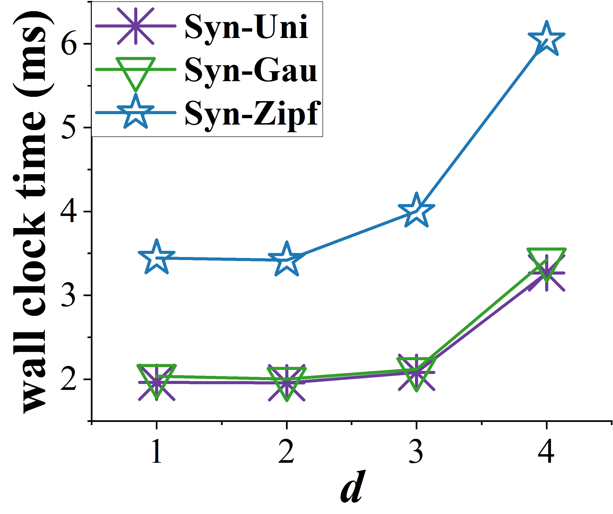
(a) DSM vs. $d$

(b) DSM vs. $\beta/\alpha$

(c) DSM vs. $m$

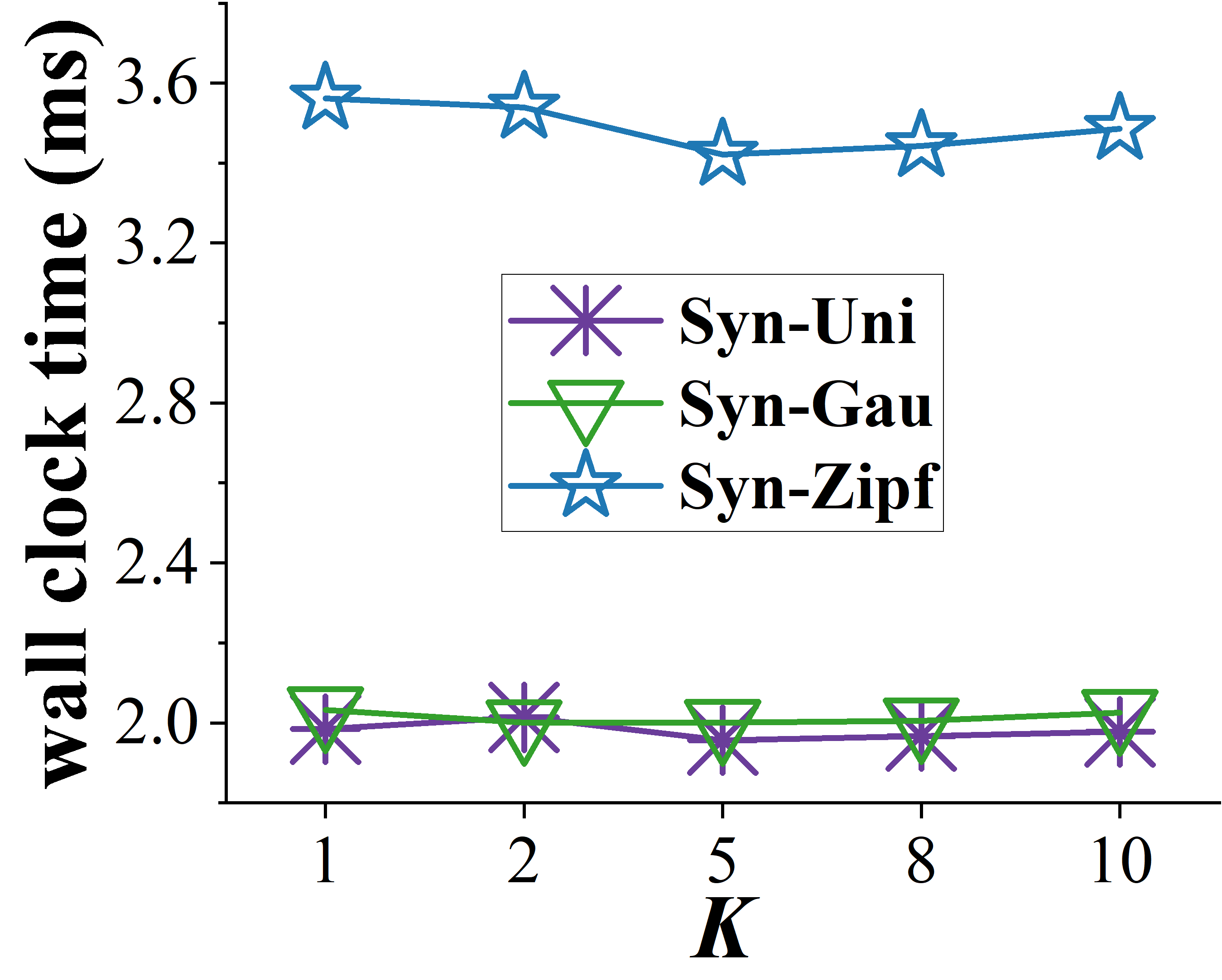
(d) DSM vs. $K$

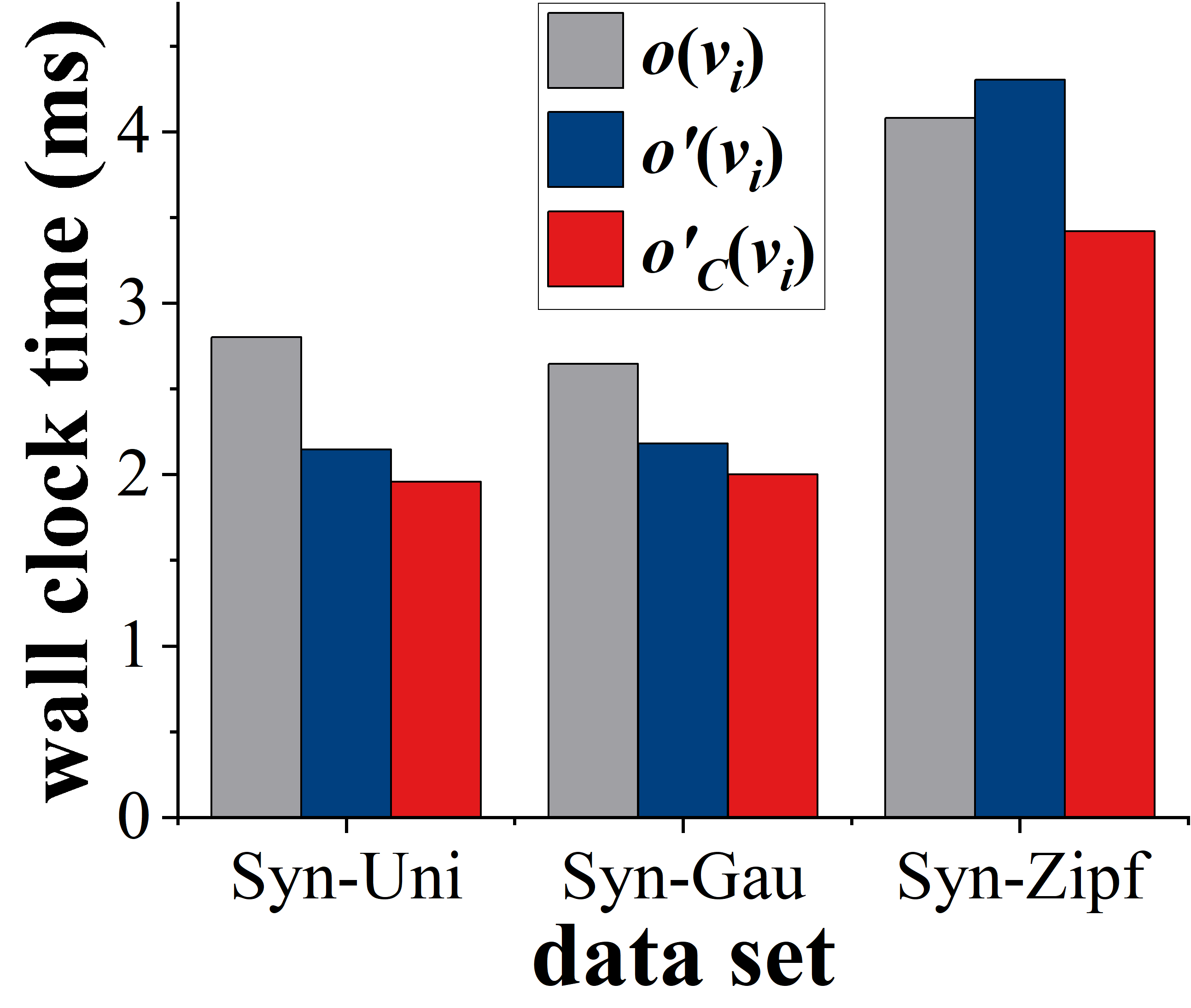
(e) DSM vs. embeddings

Figure 8. The DSM efficiency w.r.t parameters $\bm{d}$, $\bm{\beta/\alpha}$, $\bm{m}$, $\bm{K}$, and embedding design strategies.

Evaluation Metrics: In our experiments, we report the efficiency of our DSM approach and baseline methods, in terms of the wall clock time, which is the time cost of processing the DSM query over the entire graph update sequence (i.e., continuous subgraph matching answer set monitoring). In particular, this time cost includes the time of filtering, refinement, embedding updates, and synopsis updates for each DSM query. We also evaluate the pruning power of our embedding dominance pruning and MBR range pruning strategies (as mentioned in Section 6.1), which is defined as the percentage of vertices that can be ruled out by our pruning methods. For all the experiments, we take an average of each metric over 100 runs (w.r.t. 100 query graphs, resp.).

Table 3 depicts parameter settings in our experiments, where default parameter values are in bold. For each set of experiments, we vary the value of one parameter while setting other parameters to their default values.

(a) real-world graphs

(b) synthetic graphs

Figure 9. The DSM pruning power w.r.t different design strategies of vertex dominance embeddings.

(a) real-world graphs (10%)

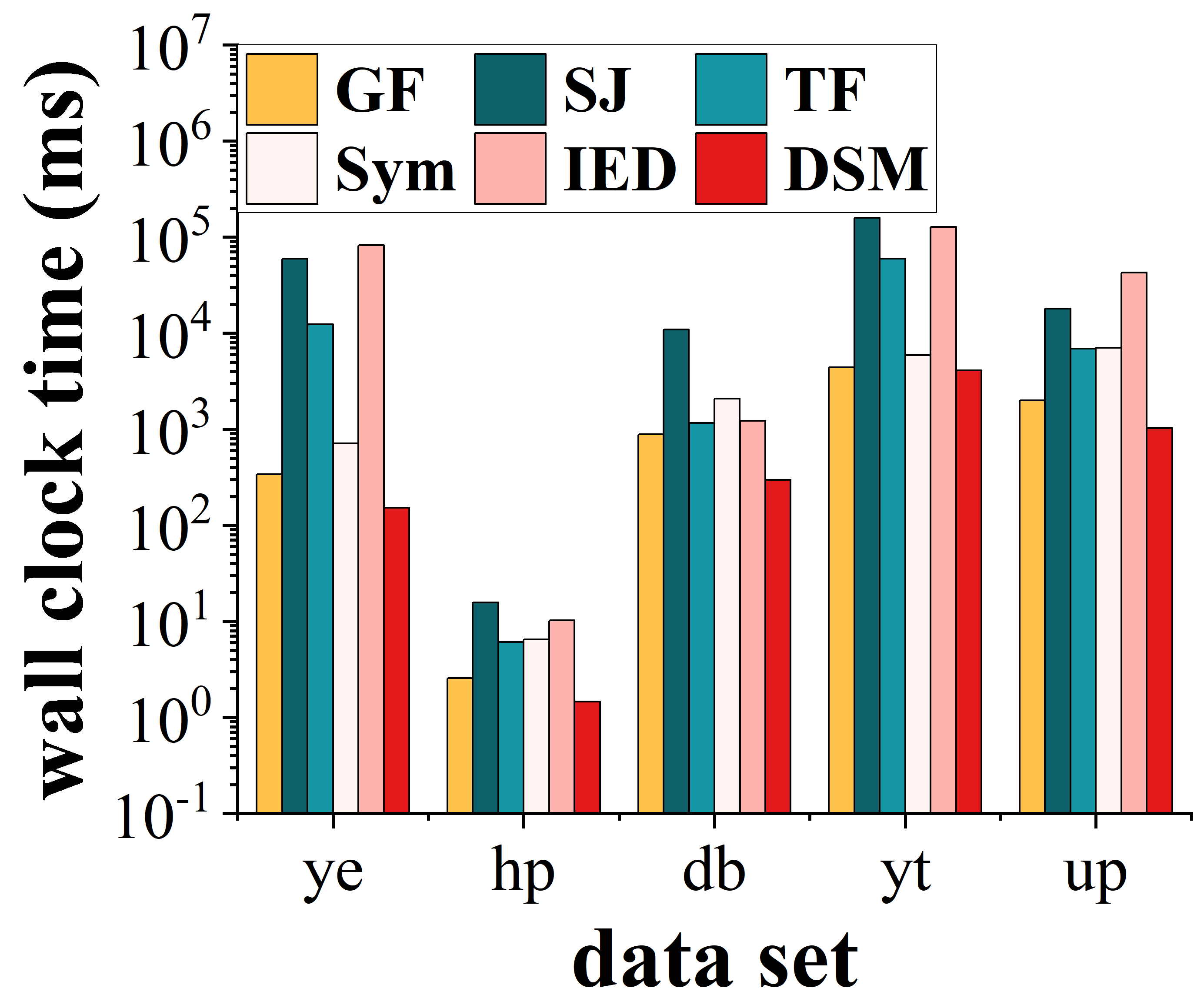
(b) real-world graphs (20%)

(c) real-world graphs (30%)

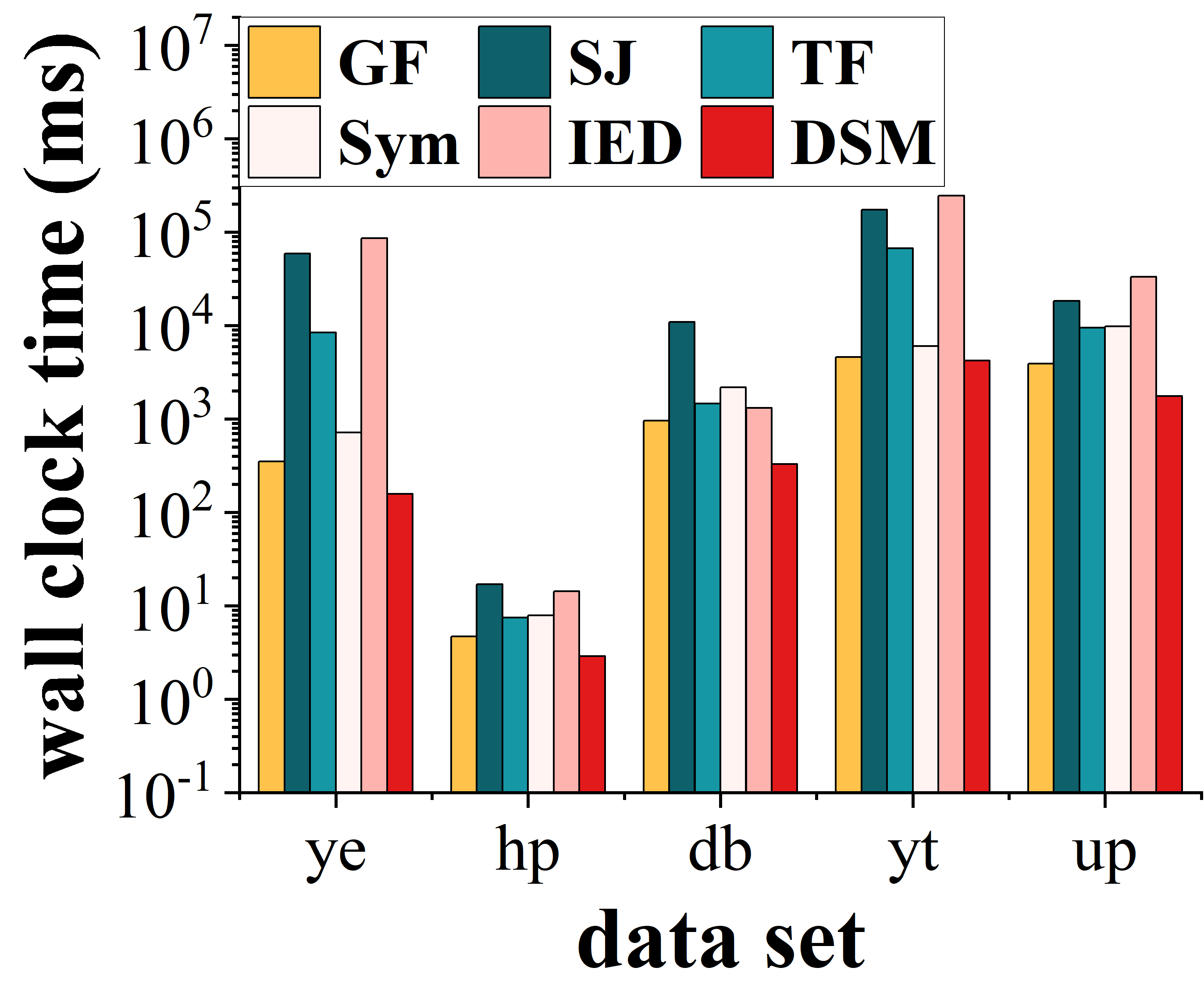
(d) real-world graphs (40%)

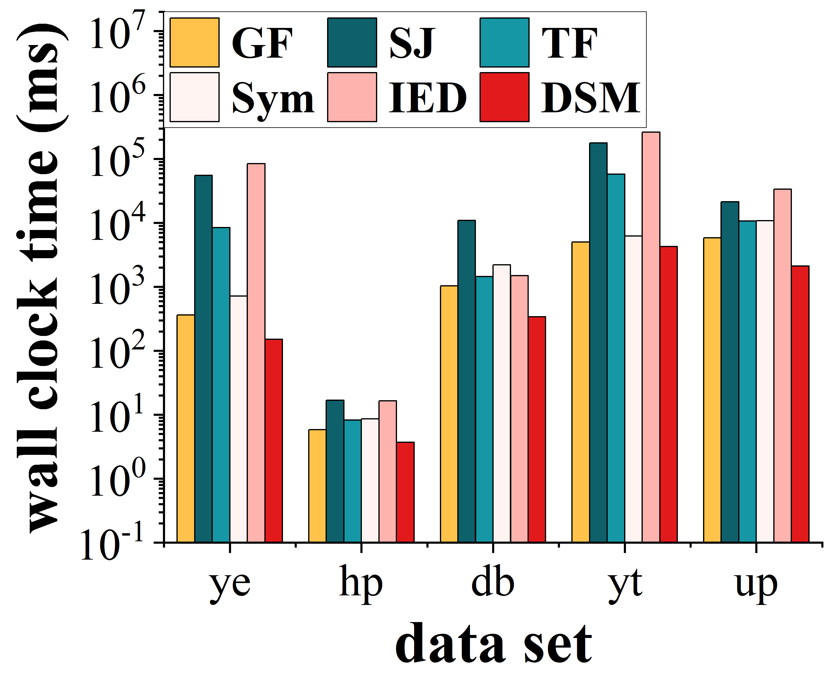
(e) real-world graphs (50%)

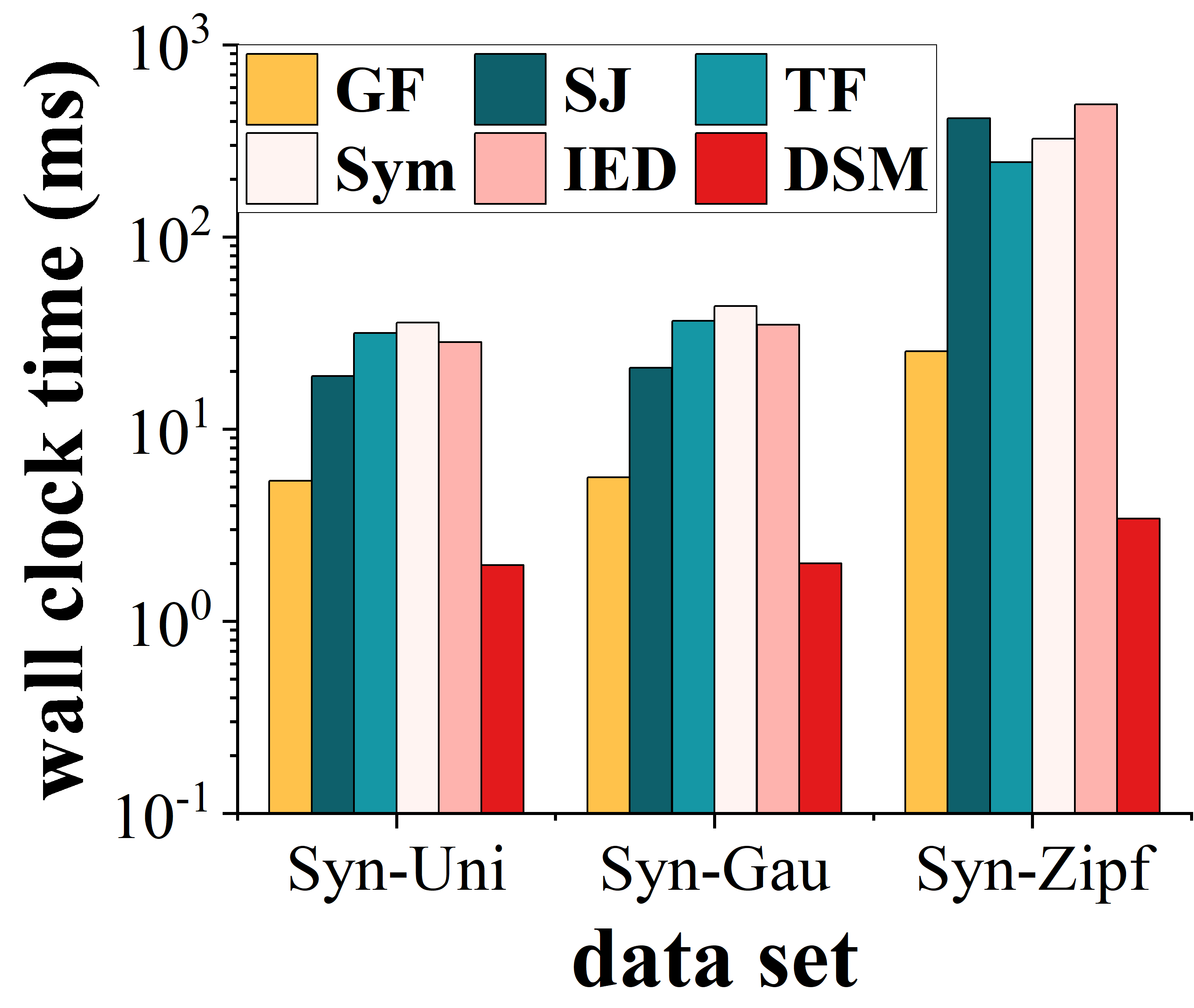
(f) synthetic graphs (10%)

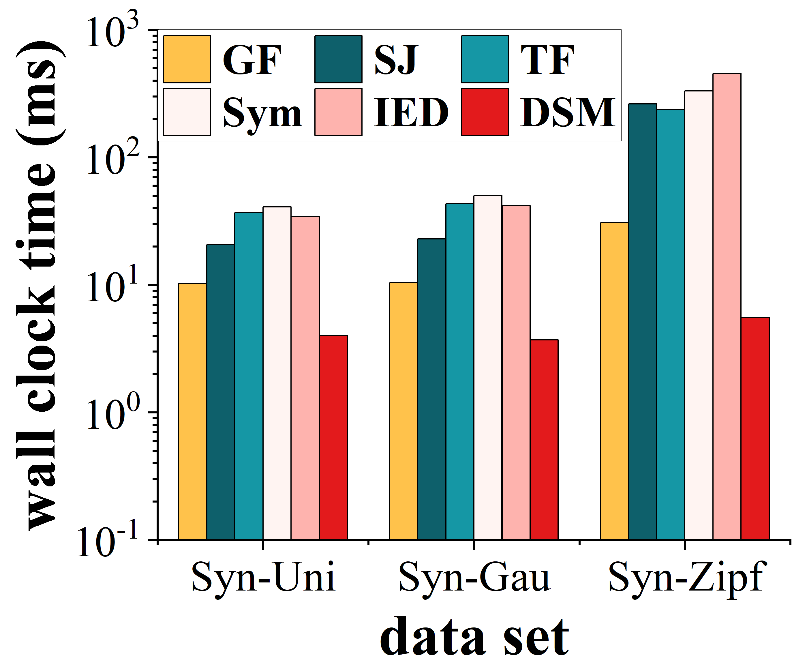
(g) synthetic graphs (20%)

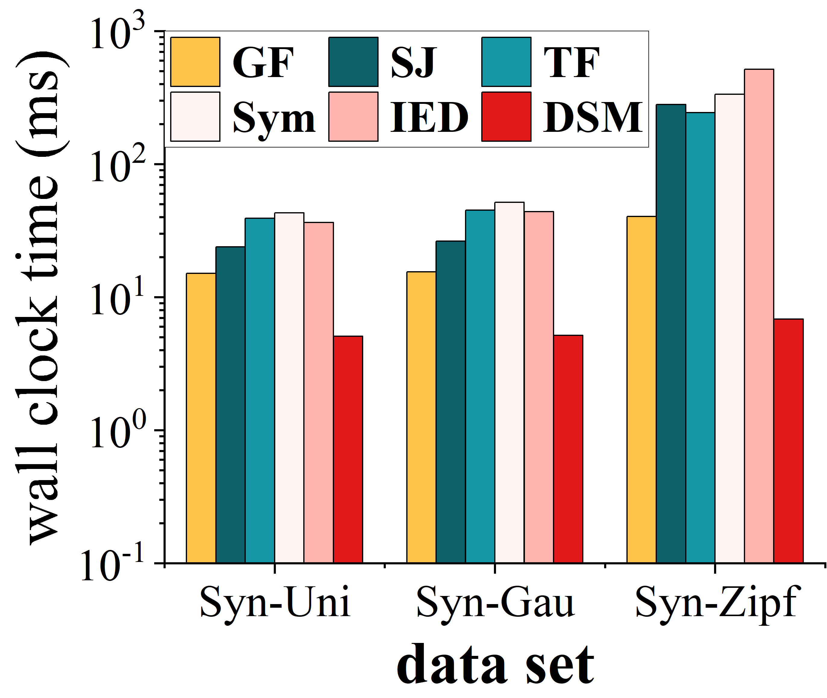
(h) synthetic graphs (30%)

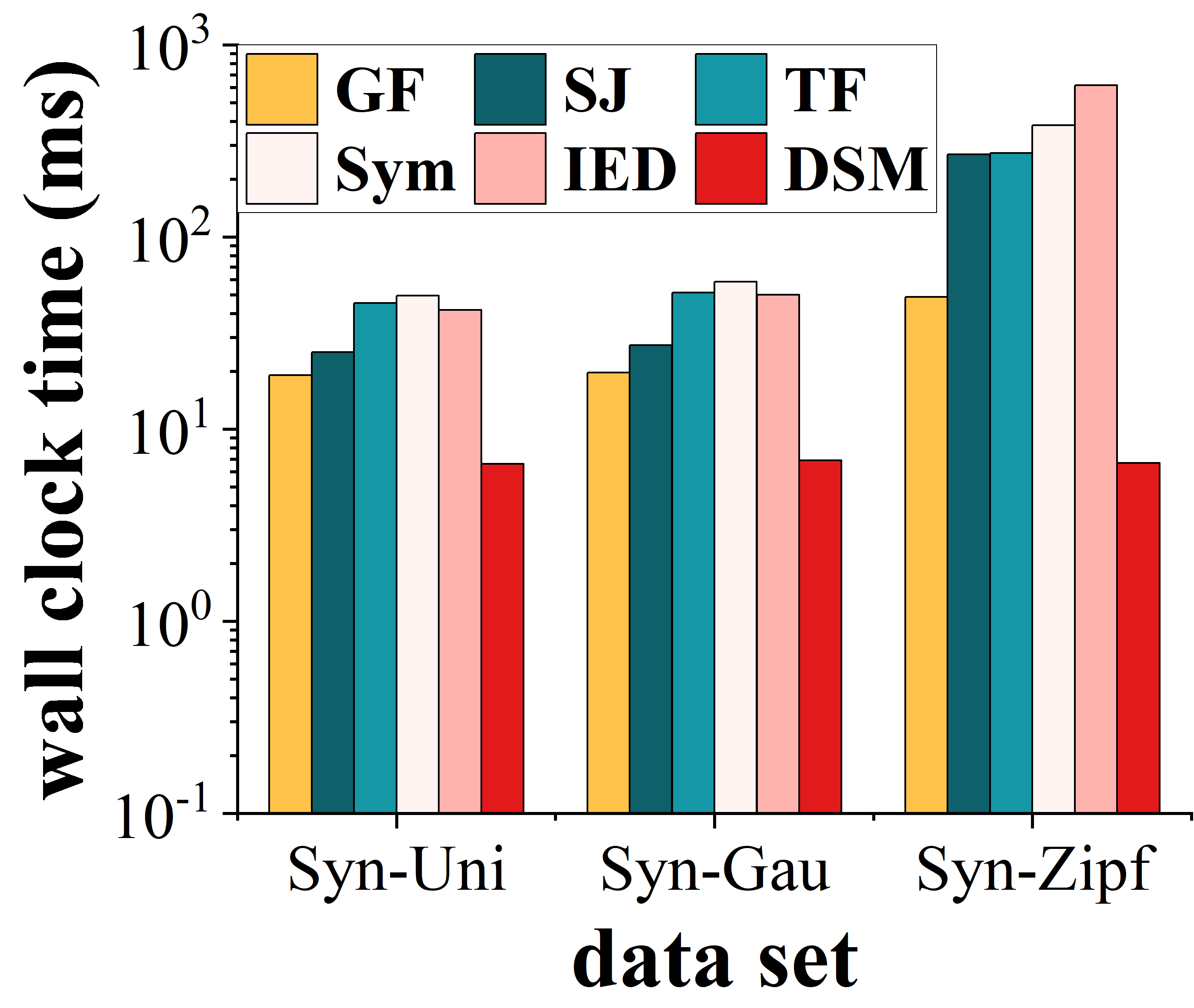
(i) synthetic graphs (40%)

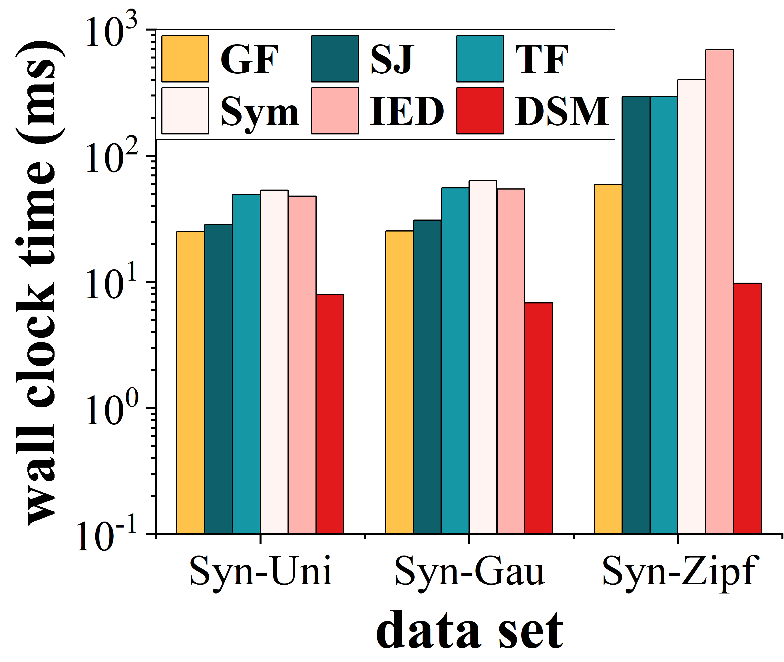
(j) synthetic graphs (50%)

Figure 10. The DSM efficiency on edge-insertion-only real/synthetic graphs, compared with baseline methods.

(a) real-world graphs (10%)

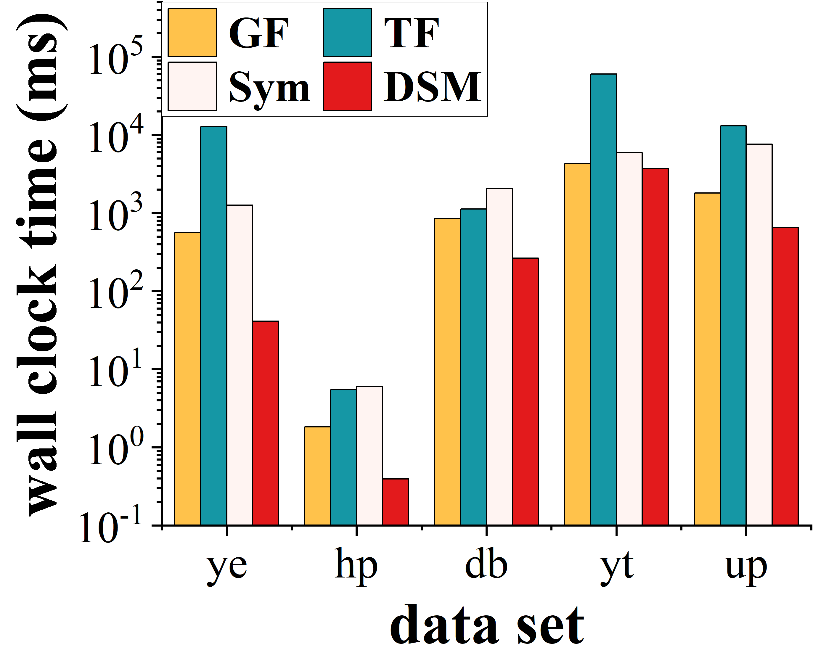
(b) real-world graphs (20%)

(c) real-world graphs (30%)

(d) real-world graphs (40%)

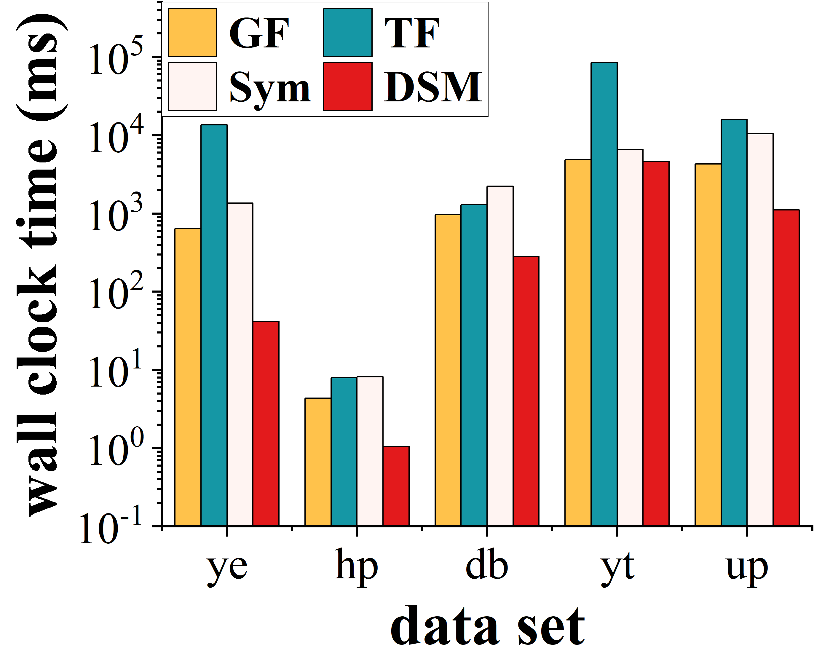
(e) real-world graphs (50%)

(f) synthetic graphs (10%)

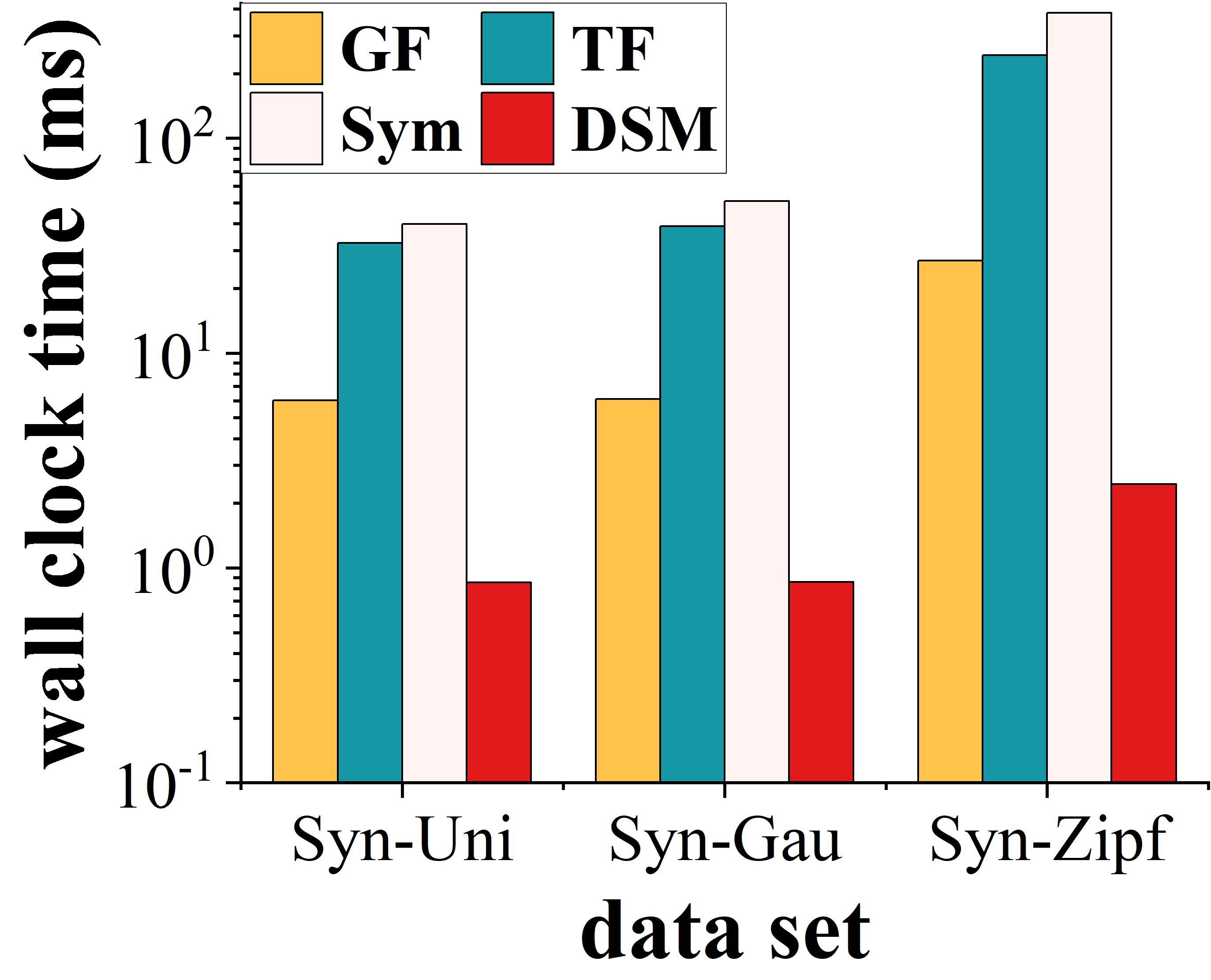
(g) synthetic graphs (20%)

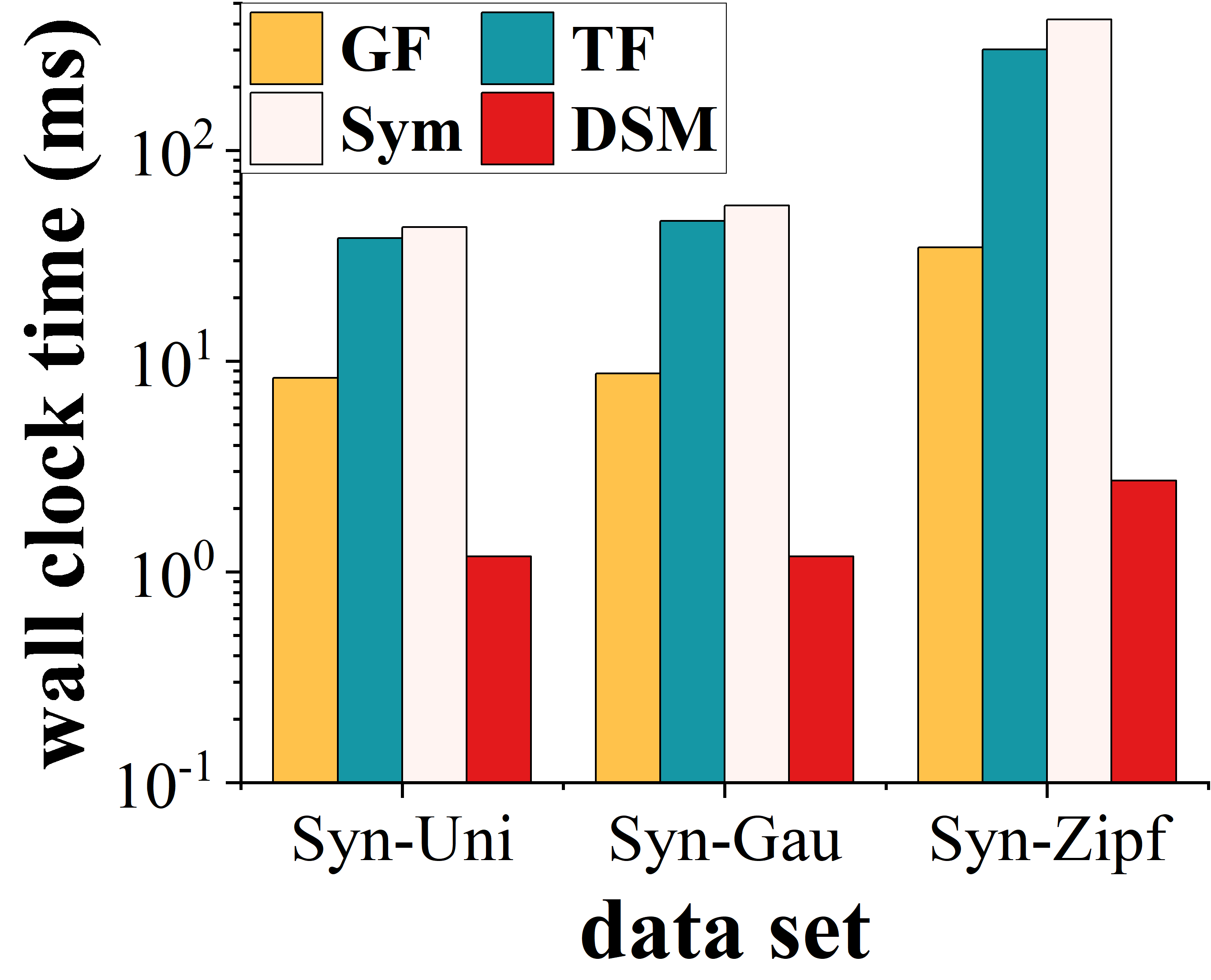
(h) synthetic graphs (30%)

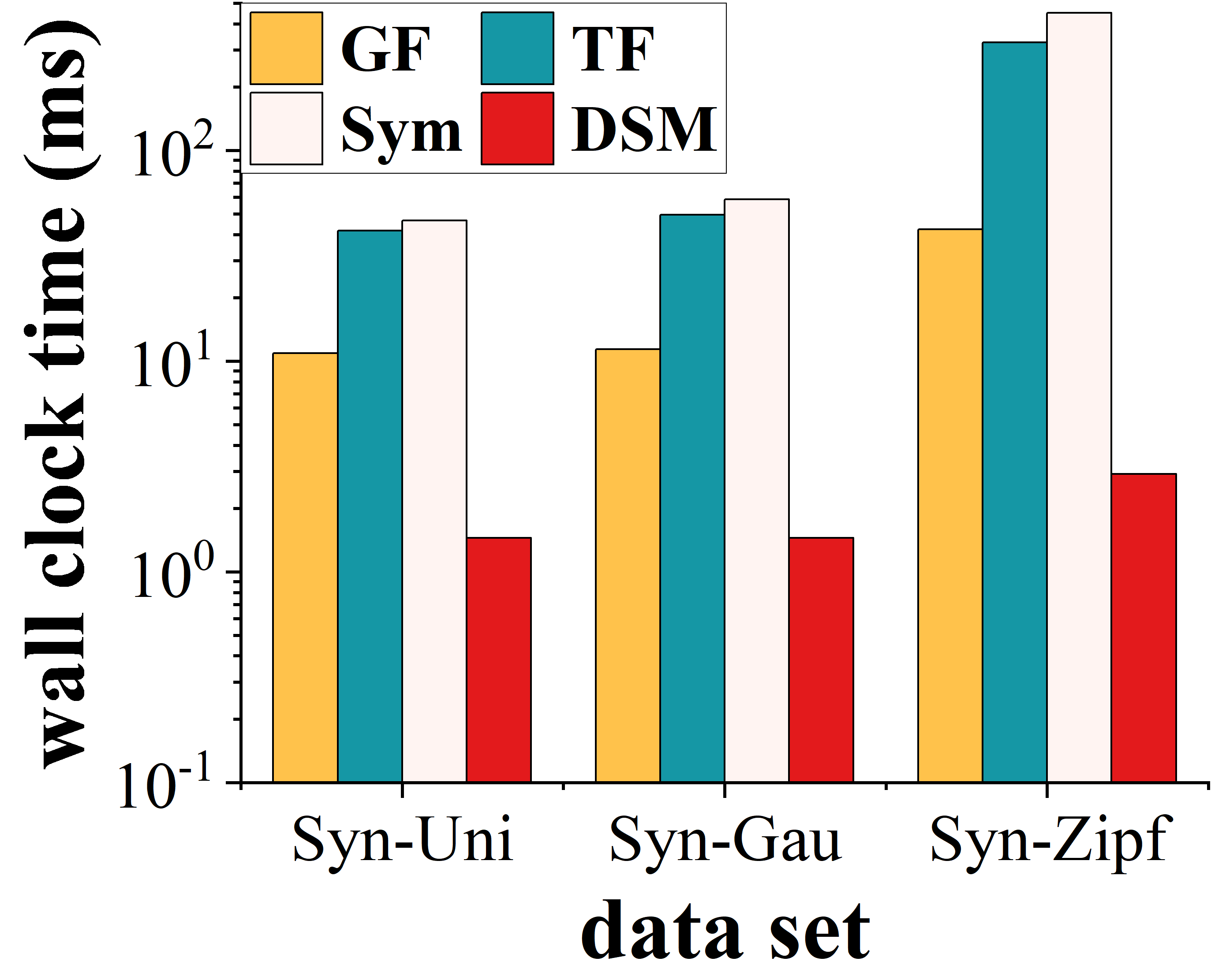
(i) synthetic graphs (40%)

(j) synthetic graphs (50%)

Figure 11. The DSM efficiency on edge-deletion-only real/synthetic graphs, compared with baseline methods.

8.2. Parameter Tuning

In this subsection, we tune parameters for our DSM approach over synthetic graphs.

The DSM Efficiency w.r.t. SPUR/SPAN Vector Dimension $\bm{d}$: Figure 8(a) illustrates the DSM performance by varying the dimension, $d$, of the cost-model-based SPUR/SPAN vector (in $o^{\prime}_{C}(v_{i})$ of Eq. (11)) from 1 to 4, where other parameters are set to their default values. With higher embedding dimension $d$, the pruning power of our proposed pruning strategies in higher dimensional space increases. However, the access of synopses with larger $d$ may also incur higher costs due to the ”dimensionality curse” (Berchtold et al., 1996). Thus, in this figure, for larger $d$, the wall clock time of DSM first decreases and then increases over all synthetic graphs. Nonetheless, the time cost remains low (i.e., 1.96 $\sim$ 6.05 $ms$) for different $d$ values.

The DSM Efficiency w.r.t. $\bm{\beta/\alpha}$ Ratio: Figure 8(b) varies the ratio, $\beta/\alpha$, from 10 to 100,000 for the optimized (or cost-model-based) vertex dominance embeddings $o^{\prime}(v_{i})$ (or $o^{\prime}_{C}(v_{i})$), where other parameters are set by default. In the figure, we can see that our DSM approaches are not very sensitive to the ratio $\beta/\alpha$. For different $\beta/\alpha$ ratios, the query cost remains low (i.e., 1.96 $\sim$ 3.75 $ms$).

The DSM Efficiency w.r.t. $\#$ of Degree Groups, $\bm{m}$: Figure 8(c) reports the performance of our DSM approach, by varying the number, $m$, of degree groups from 1 to 5, where other parameters are set by default. In this figure, the time costs over $Syn\text{-}Uni$ and $Syn\text{-}Zipf$ first decrease and then increase when $m$ increases, and there are some fluctuations for $Syn\text{-}Gau$ (e.g., for $m=4$ or $5$). For all $m$ values, the time cost remains low (i.e., 1.94 $\sim$ 3.74 $ms$).

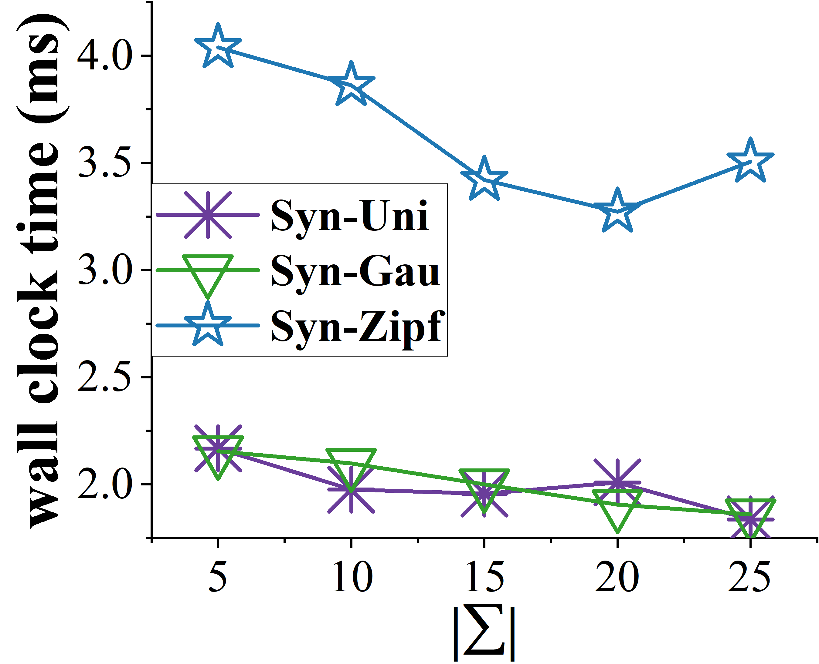
(a) DSM vs. $|\Sigma|$

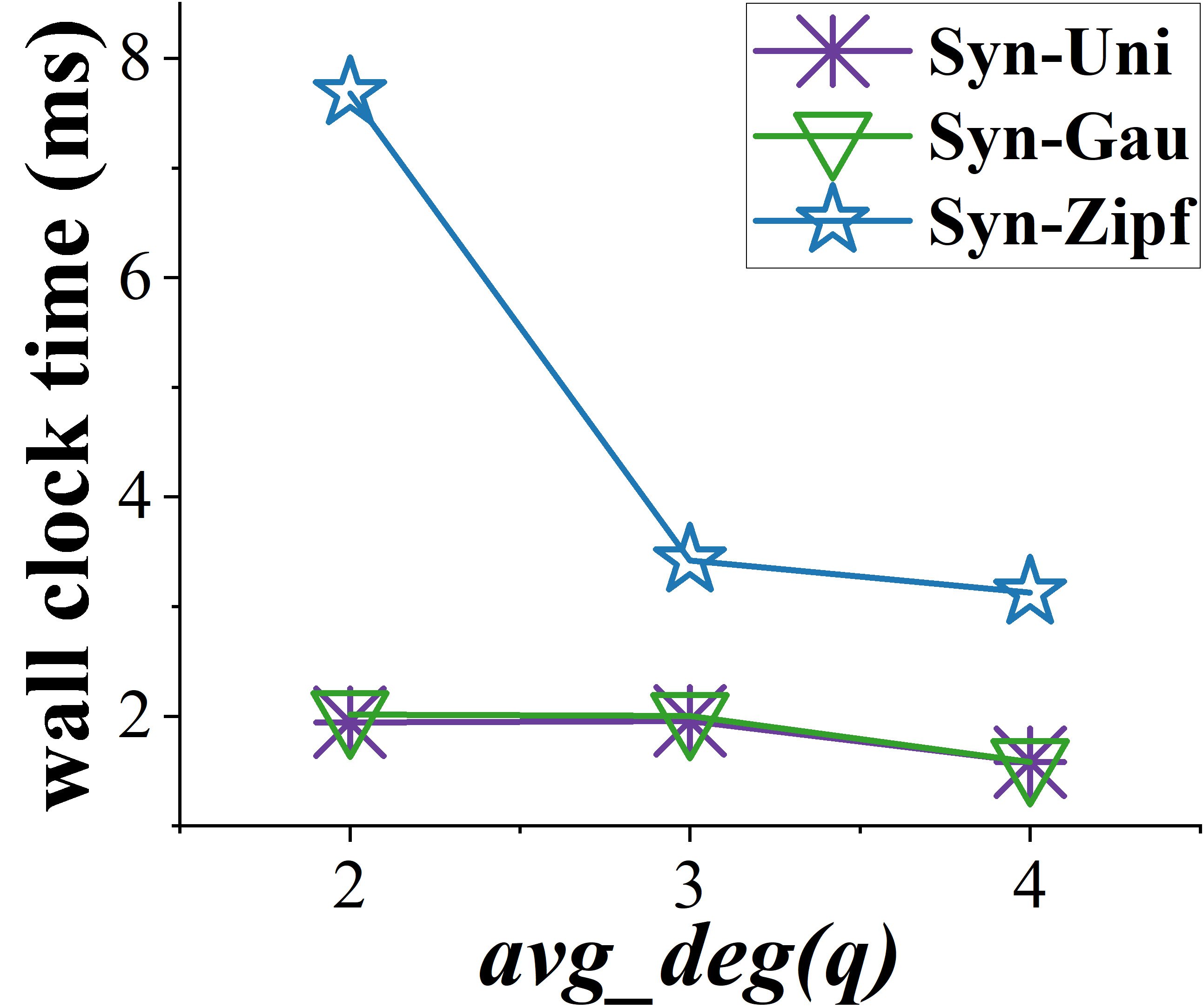
(b) DSM vs. $avg\_deg(q)$

(c) DSM vs. $|V(q)|$

(d) DSM vs. $avg\_deg(G_{D})$

(e) DSM vs. $|V(G_{D})|$

Figure 12. The DSM efficiency w.r.t. parameters $|\Sigma|$, $avg\_deg(q)$, $|V(q)|$, $avg\_deg(G_{D})$, and $|V(G_{D})|$.

The DSM Efficiency w.r.t. $\#$ of Cell Intervals on Each Dimension, $\bm{K}$: Figure 8(d) evaluates the effect of the number, $K$, of cell intervals on each dimension on the DSM performance, where $K$ varies from 1 to 10, and other parameters are set by default. When $K$ becomes larger, more vertices in synopsis cells can be pruned, however, more cells need to be accessed. Therefore, for DSM, with the increase of $K$, the time cost first decreases and then increases. Nonetheless, for different $K$ values, the query cost remains low (i.e., 1.96 $\sim$ 3.54 $ms$).

The DSM Efficiency w.r.t. Vertex Dominance Embedding Design Strategy: Figure 8(e) tests the DSM performance with different designs of vertex dominance embeddings, $o(v_{i})$ (in Eq. (3)), $o^{\prime}(v_{i})$ (in Eq. (4)), and $o^{\prime}_{C}(v_{i})$ (in Eq. (11)), where default values are used for parameters. In the figure, we can see that, the optimized vertex embeddings $o^{\prime}(v_{i})$ (via the base vector $z_{i}$) incur smaller time cost than $o(v_{i})$ in all cases, whereas the cost-model-based vertex embeddings $o^{\prime}_{C}(v_{i})$ consistently achieve the lowest time. For different vertex embeddings, the query cost remains low (i.e., 1.96$\sim$4.3$ms$).

The experimental results on real-world graphs are similar and thus omitted here. In subsequent experiments, we will set parameters $d=2$, $\beta/\alpha=1,000$, $m=3$, and $K=5$, and use the cost-model-based vertex embeddings $o^{\prime}_{C}(v_{i})$ (given by Eq. (11)).

8.3. The DSM Effectiveness Evaluation

In this subsection, we report the pruning power of our proposed pruning strategies (as discussed in Section 6.1) for dynamic subgraph matching queries over real/synthetic graphs.

The DSM Pruning Power on Real/Synthetic Graphs: Figure 9 shows the pruning power of our DSM approach over real/synthetic graphs with different embedding designs $o(v_{i})$, $o^{\prime}(v_{i})$, and $o^{\prime}_{C}(v_{i})$, where all parameters are set by default. In figures, we can see that for all real/synthetic graphs, the pruning power of our proposed vertex embedding designs can reach as high as $94.47\%\sim 99.58\%$ for real-world graphs and $85.99\%\sim 98.65\%$ for synthetic graphs, which confirms the effectiveness of our embedding-based pruning strategies. Our cost-model-based vertex embedding strategy $o^{\prime}_{C}(v_{i})$ always achieves the highest pruning power (i.e., $86.93\%\sim 99.58\%$).

8.4. The DSM Efficiency Evaluation

In this subsection, we report the efficiency of our DSM approaches over real/synthetic graphs.

The DSM Efficiency on Edge-Insertion-Only Real/Synthetic Graphs: Figure 10 compares the efficiency of our DSM approach with that of 5 state-of-the-art baseline methods by varying the insertion ratio from 10% to 50% over both real and synthetic graphs, where all other parameters are set to default values. In Figures 10(a) and 10(f) with the default 10% insertion ratio, we can see that our DSM approach outperforms baseline methods mostly by 1-2 orders of magnitude. Overall, for all graphs (even for $up$ with $3.77M$ vertices and $1.65M$ edge insertions), the time cost of our DSM approach remains low (i.e., $<$$3.91$ $sec$).

For other subfigures with different insertion ratios from 20% to 50%, we can see similar experimental results over both real and synthetic graphs. Although the total query time will increase as the number of inserted edges increases, our DSM approach can achieve performance that is up to 1-2 orders of magnitude than baseline methods. In summary, for all insertion ratios and graphs (even for $up$ with $3.77M$ vertices and $8.26M$ edge insertions), the time cost of our DSM approach remains low (i.e., $<4.37$ $sec$).

The DSM Efficiency on Edge-Deletion-Only Real/Synthetic Graphs: Since SJ and IED baselines do not support the edge deletion (Sun et al., 2022a), Figure 11 only compares the efficiency of our DSM approach with that of GF, TF, and SYM over real/synthetic graphs, where the deletion ratio varies from 10% to 50% and all other parameters are set to their default values. From Figures 11(a) and 11(f) with the default 10% deletion ratio, our DSM approach can always outperform the three baseline methods. Overall, for all real/synthetic data sets (even for $up$ with 1.65$M$ edge deletions), the wall clock time of our DSM approach remains low (i.e., $<3.55$ $sec$).

From other subfigures with different deletion ratios 20% $\sim$ 50%, we can find similar experimental results over both real and synthetic graphs, where our DSM approach can always outperform the three baseline methods. For different edge deletion ratios and graph sizes (even for $up$ with $3.77M$ vertices and $8.26M$ edge deletions), the time cost of our DSM approach remains low (i.e., $<4.62$ $sec$).

To evaluate the robustness of our DSM approaches, in the sequel, we vary the parameter values on synthetic graphs (e.g., $|\Sigma|$, $avg\_deg(q)$, $|V(q)|$, $avg\_deg(G_{D})$, and $|V(G_{D})|$). To better illustrate the trends of curves, we omit the results of the baselines below.

The DSM Efficiency w.r.t. $\#$ of Distinct Vertex Labels, $\bm{|\Sigma|}$: Figure 12(a) shows the wall clock time of our DSM approach, where $|\Sigma|$ varies from 5 to 25, and other parameters are set to default values. When the number, $|\Sigma|$, of distinct vertex labels increases, the pruning power also increases (i.e., with fewer candidate vertices). Moreover, the query cost is also affected by vertex label distributions. Overall, the DSM query cost remains low for different $|\Sigma|$ values (i.e., 1.83 $\sim$ 4.04 $ms$).

The DSM Efficiency w.r.t. Average Degree, $\bm{avg\_deg(q)}$, of the Query Graph $\bm{q}$: Figure 12(b) examines the DSM performance by varying the average degree, $avg\_deg(q)$, of the query graph $q$ from 2 to 4, where other parameters are set to default values. Higher degree $avg\_deg(q)$ of $q$ incurs higher pruning power of query vertices. Therefore, when $avg\_deg(q)$ increases, the DSM time cost decreases. For different $avg\_deg(q)$ values, the DSM query cost remains low (i.e., 1.58 $\sim$ 7.68 $ms$).

The DSM Efficiency w.r.t. Query Graph Size $\bm{|V(q)|}$: Figure 12(c) illustrates our DSM performance, by varying the query graph size, $|V(q)|$, from 5 to 12, where default values are used for other parameters. When the number, $|V(q)|$, of vertices in query graph $q$ increases, fewer candidate subgraphs are expected to match with larger query graph $q$. On the other hand, larger query graph size $|V(q)|$ will cause higher query costs in finding candidates for more query vertices, through synopsis traversal and refinement. Thus, the query time is influenced by these two factors. Nevertheless, the time cost remains low for different query graph sizes (i.e., $<$$5.36$$ms$).

The DSM Efficiency w.r.t. Avg. Degree, $\bm{avg\_deg(G_{D})}$, of Dynamic Graph $\bm{G_{D}}$: Figure 12(d) presents our DSM performance with different average degrees, $avg\_deg$ $(G_{D})$, of dynamic graph $G_{D}$, where $avg\_deg(G_{D})=3\sim 7$, and default values are used for other parameters. Intuitively, higher degree $avg\_deg(G_{D})$ in data graph $G_{D}$ incurs lower pruning power and more candidate vertices. Thus, when $avg\_deg(G_{D})$ becomes higher, the wall clock time also increases, especially for $Syn\text{-}Zipf$ (due to its skewed vertex label distribution). Nevertheless, the DSM query time remains small for different $avg\_deg(G_{D})$ values (i.e., 1.08 $\sim$ 5.82 $ms$).

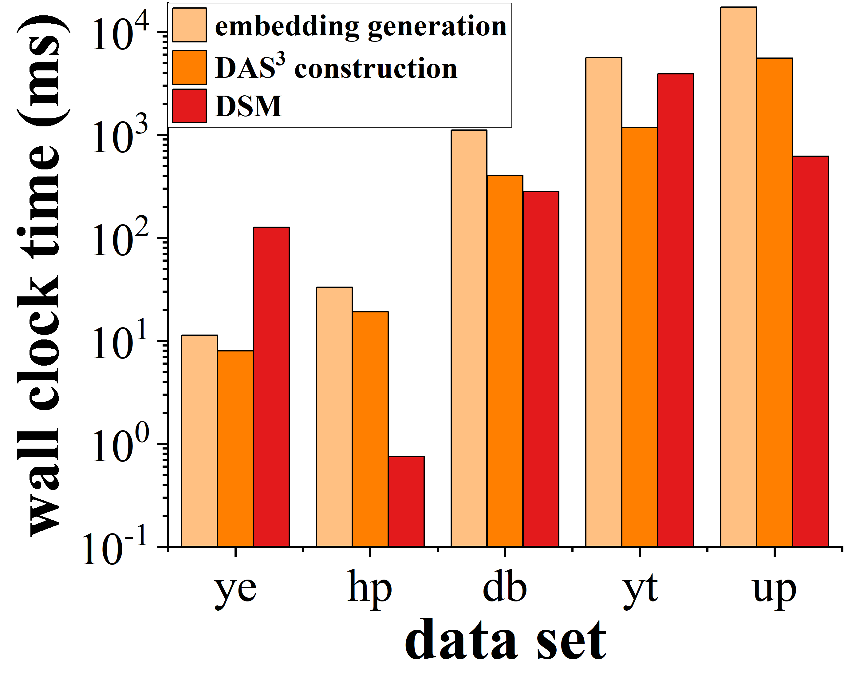
(a) real-world graphs

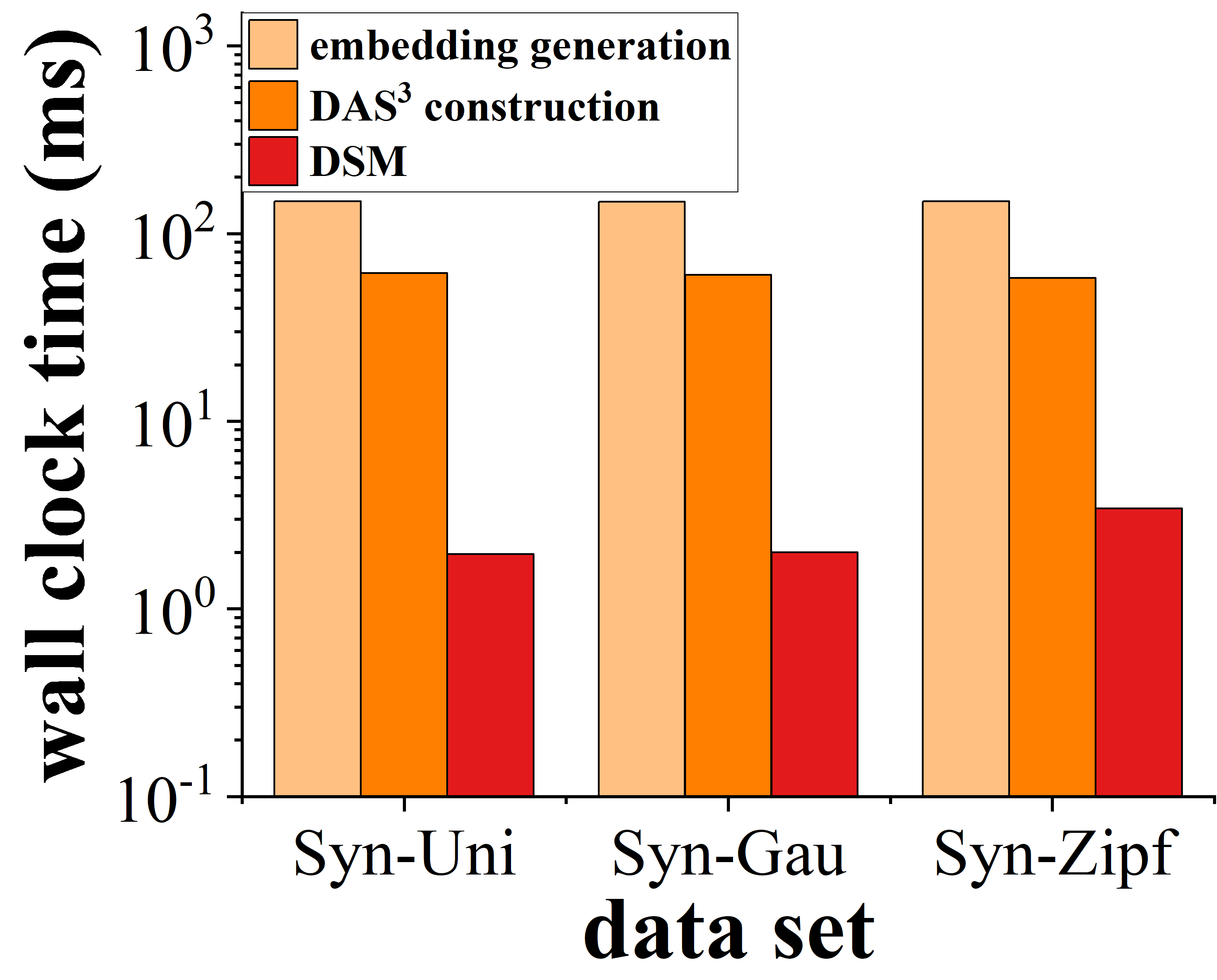
(b) synthetic graphs

Figure 13. The comparison analysis of the DSM offline pre-computation and online query costs on real/synthetic graphs.

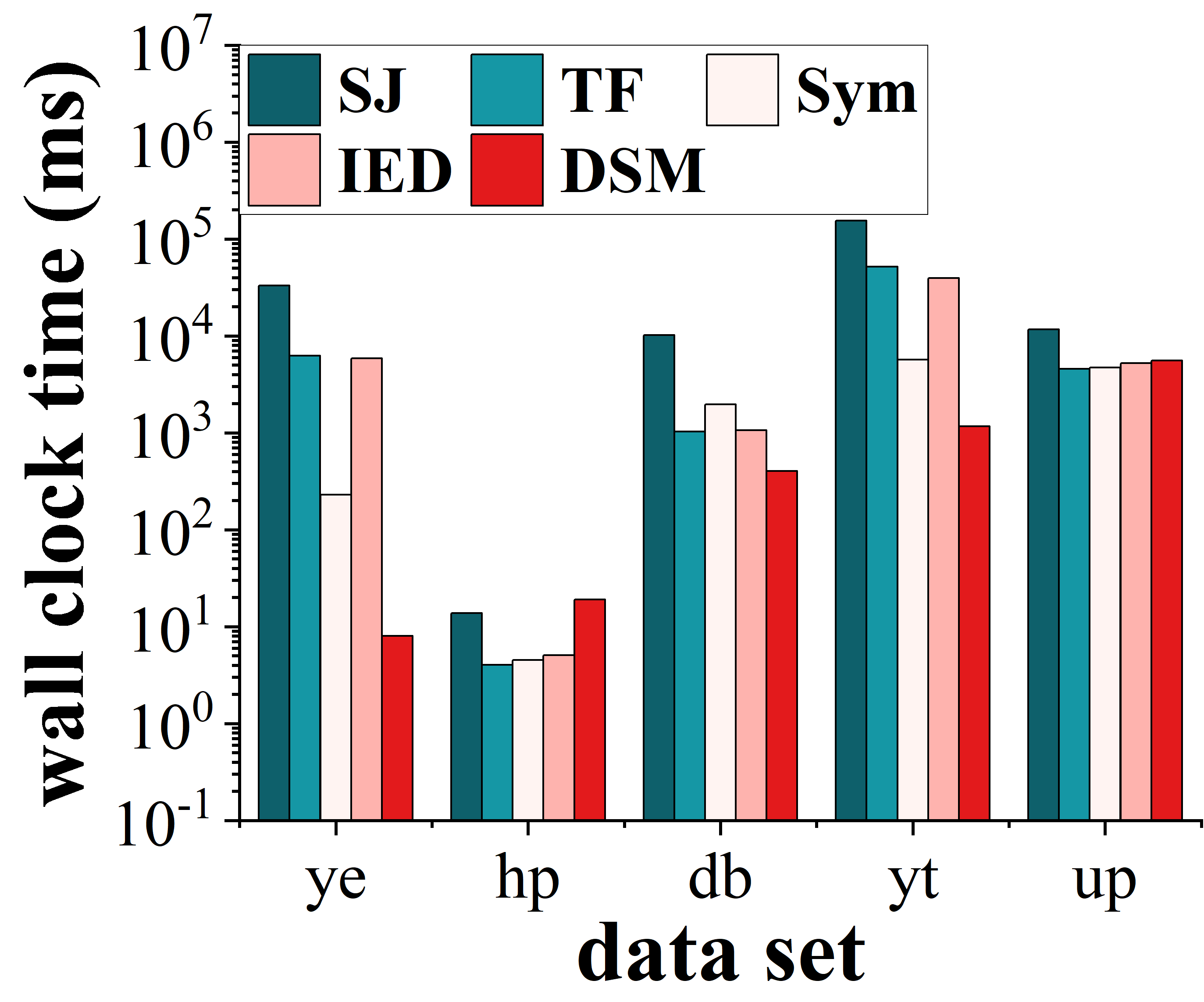
(a) real-world graphs

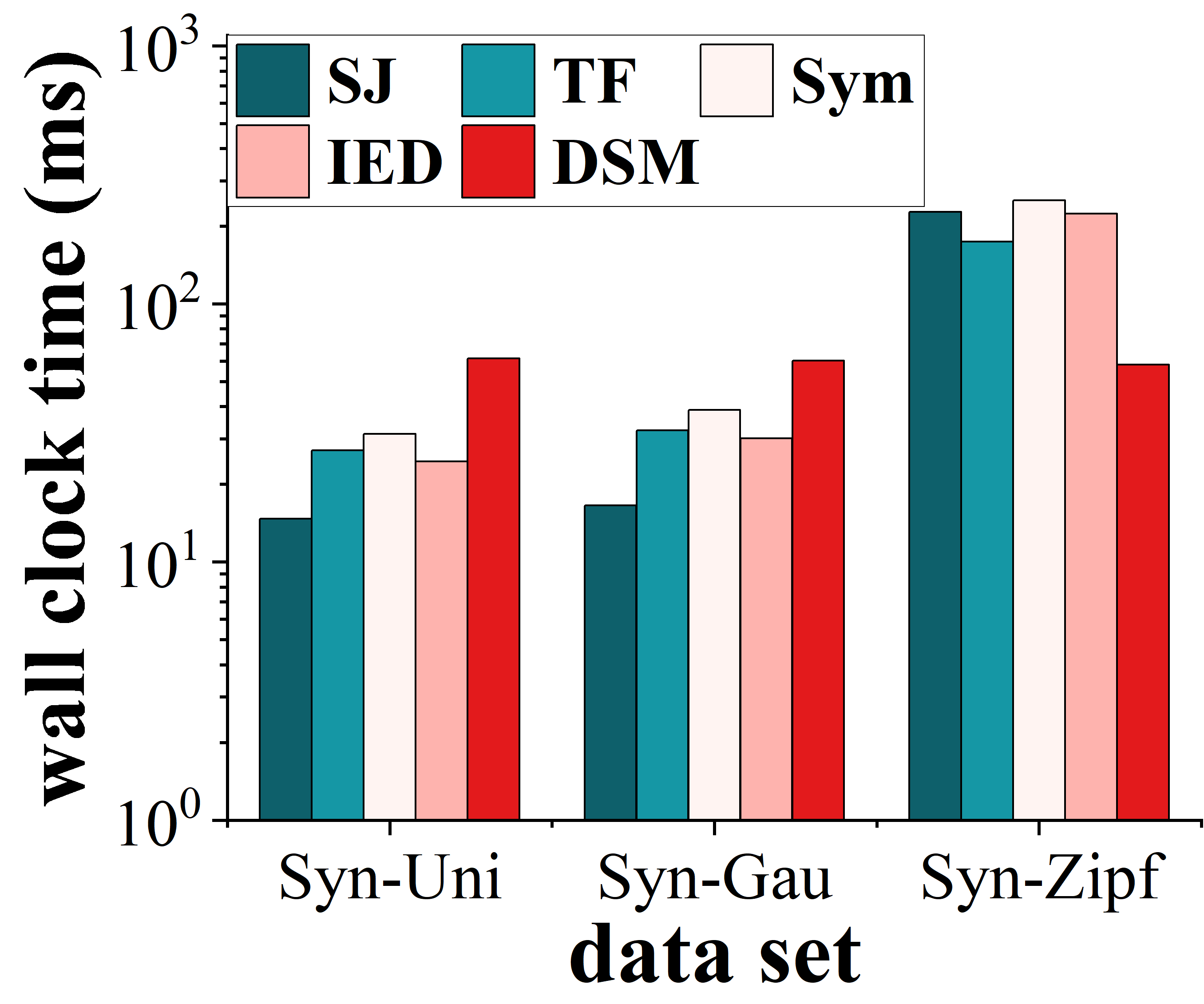
(b) synthetic graphs

Figure 14. DAS³ construction time on real/synthetic graphs, compared with baseline methods.

The DSM Scalability Test w.r.t. Dynamic Graph Size $\bm{|V(G_{D})|}$: Figure 12(e) tests the scalability of our DSM approach with different dynamic graph sizes, $|V(G_{D})|$, from $10K$ to $1M$, where default values are assigned to other parameters. A larger dynamic graph incurs more matching candidate vertices (and, in turn, candidate subgraphs). From this figure, the time cost of DSM increases linearly with the increase of graph size $|V(G_{D})|$, nonetheless, remains low (i.e., 0.4 $\sim$ 104.62 $ms$), which confirms the scalability of our DSM approach for large graph sizes.

8.5. DAS³ Synopsis Initialization Cost

The DAS³ Synopsis Initialization Cost on Real/Synthetic Graphs. We compare the DAS³ synopsis initialization cost of our DSM approach (including time costs of vertex dominance embedding generation and DAS³ construction over vertex dominance embeddings) with online query time over real/synthetic graphs, where parameters are set to default values. In Figure 13, for graph size from 3K to 3.77M, the overall offline pre-computation time varies from 19 $ms$ $\sim$ 23 $sec$. Specifically, the time costs of embedding generation and DAS³ construction are 11 $ms$ $\sim$ 17 $sec$, 8 $ms$ $\sim$ 6 $sec$, respectively. On the other hand, since the online query time includes the time cost of DAS³ and embedding update, the maintenance cost of our DAS³ is low.

(a) real-world graphs

(b) synthetic graphs

Figure 15. DAS³ memory cost on real/synthetic graphs, compared with baseline methods.

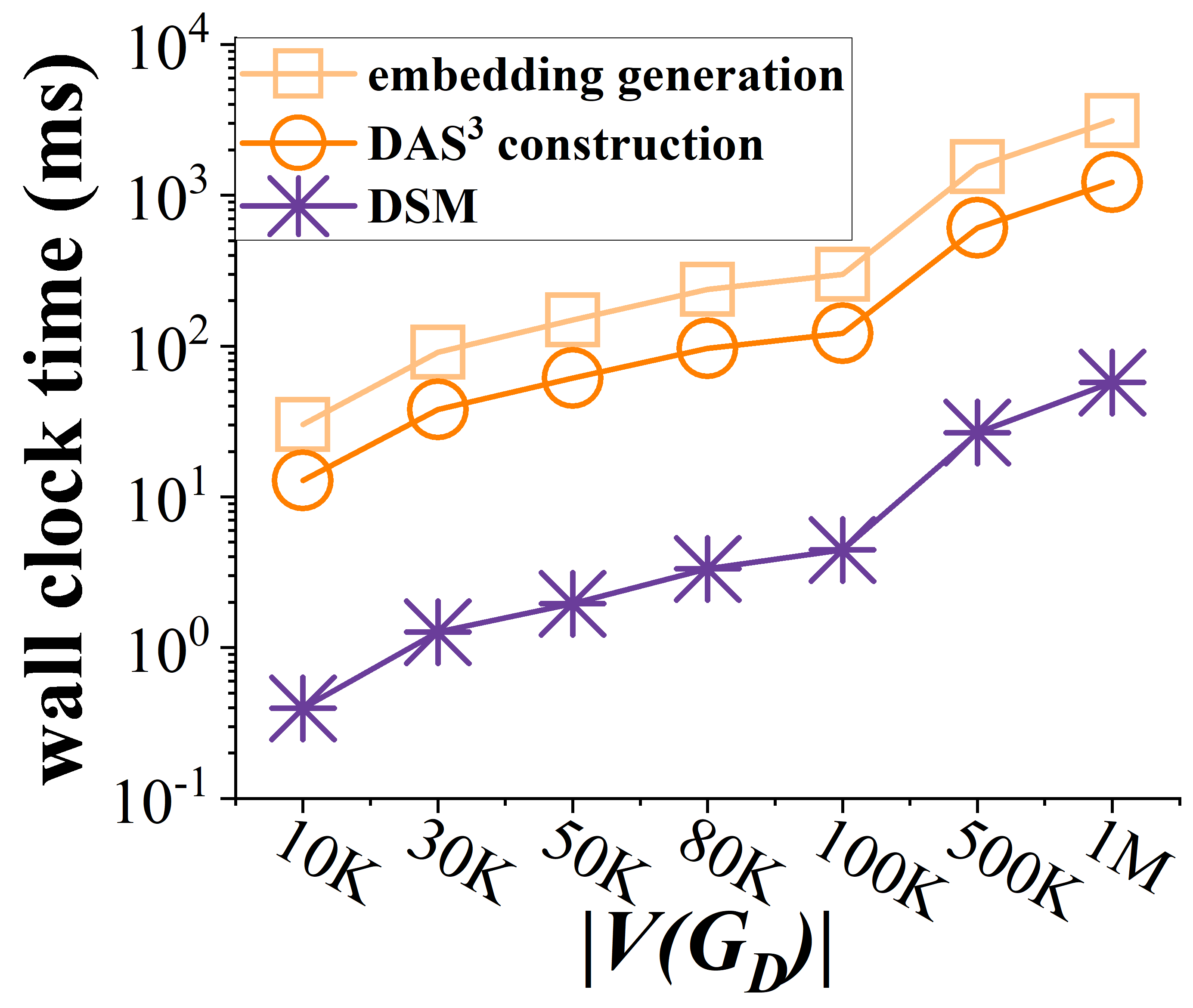
(a) $Syn\text{-}Uni$

(b) $Syn\text{-}Gau$

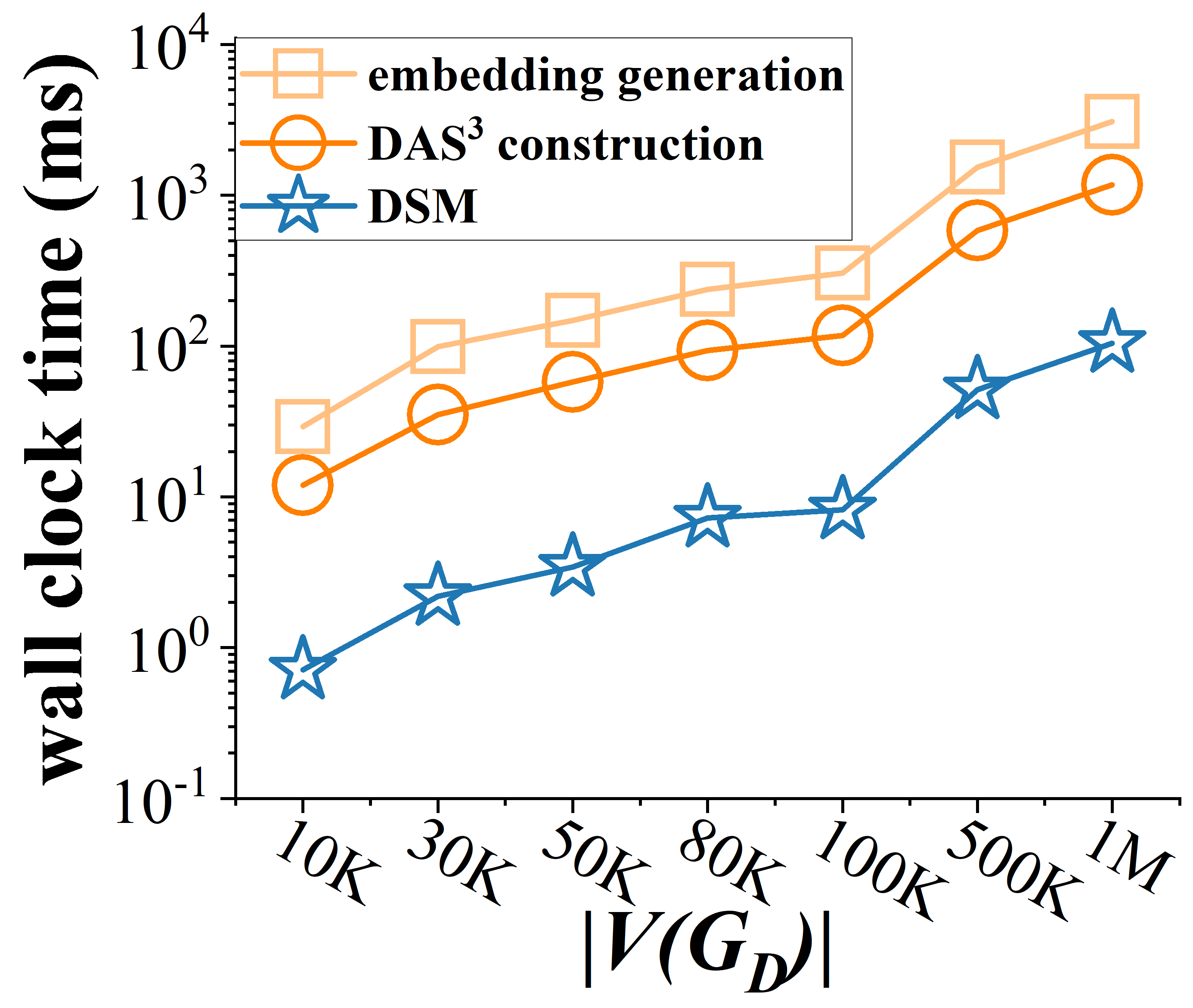
(c) $Syn\text{-}Zipf$

Figure 16. The DSM pre-computation and query costs w.r.t data graph size $|V(G_{D})|$.

The DAS³ Index Time/Space Cost on Real/Synthetic Graphs. Since GF directly enumerates matching answers over the original data graph without any auxiliary data structure (Kankanamge et al., 2017; Sun et al., 2022a), Figures 14 and 15 compare the construction time and storage cost of our DAS³ with the other 4 baselines, where parameters are set to their default values. From Figure 14, we can find that our DAS³ needs shorter construction time over some complex graphs, i.e., ye, db, yt, and $Syn\text{-}Zipf$. This is because, different from baseline methods that build auxiliary data structure over initial query answers, our DAS³ is built over the initial data graph without enumerating the initial query answers and only depends on the data graph size. As shown in Figure 15, except SJ with exponential space cost (Choudhury et al., 2015; Sun et al., 2022a), our DAS³ needs more storage costs for storing/indexing vertex dominance embeddings. However, different from baseline methods that construct an index for each query graph during the online dynamic subgraph matching process, our DAS³ construction is offline and one-time only. Thus, our offline constructed DAS³ can be used to accelerate numerous online dynamic subgraph matching requests from users simultaneously with high throughput.

The DAS³ Synopsis Initialization Cost and Online Query Costs w.r.t. Data Graph Size $|V(G_{D})|$. Figure 16(a) evaluates the DAS³ synopsis initialization cost of our DSM approach, including time costs of the vertex dominance embedding generation and DAS³ construction over embeddings, compared with online DSM query time, over synthetic graphs $Syn\text{-}Uni$, where we vary the graph size $|V(G)|$ from $10K$ to $1M$ and other parameters are set to default values. Specifically, for graph sizes from $10K$ to $1M$, the time costs of the embedding generation and DAS³ construction are 0.03$\sim$3.11 $sec$ and 0.01$\sim$1.22 $sec$, respectively. The overall offline pre-computation time varies from 0.04 $sec$ to 4.33 $sec$, and the dynamic subgraph matching query cost is much smaller (i.e., 0.4$\sim$57.49 $ms$).

In Figures 16(b) and 16(c), we can see similar experimental results over $Syn\text{-}Gau$ and $Syn\text{-}Zipf$ graphs, respectively, where the subgraph matching query cost is much smaller than the overall offline pre-computation time.

9. Related work

Dynamic Subgraph Matching: Existing works on exact dynamic subgraph matching (Fan et al., 2013b; Choudhury et al., 2015; Kankanamge et al., 2017; Idris et al., 2017, 2020; Kim et al., 2018; Min et al., 2021) can be classified into three categories: the recomputation-based (Fan et al., 2013b), direct-incremental (Kankanamge et al., 2017), and index-based incremental algorithms (Choudhury et al., 2015; Idris et al., 2017, 2020; Kim et al., 2018; Min et al., 2021). For the recomputation-based category, IncIsoMatch (Fan et al., 2013b) extracted a snapshot subgraph $g_{S}\subseteq G_{t}$ surrounding the updated edges at the timestamp $t$, conducted the subgraph matching over this snapshot subgraph $g_{S}$ (w.r.t. query graph $q$), and updated the answer set $A(q,t-1)$ at timestamp $(t-1)$ with new subgraph matching answers by removing redundant subgraphs. For the direct-incremental approach, GraphFlow (Kankanamge et al., 2017) computed incremental results over the dynamic graph by using a multi-way join from the updated edge.

Moreover, index-based incremental methods construct an index over the initial subgraph matching answers, and obtain incremental results from the index (instead of the data graph). For example, SJ-Tree (Choudhury et al., 2015) modeled a dynamic subgraph query as a multi-way join and organized all partial join results in an index to serve the query. TurboFlux (Kim et al., 2018) built a tree index in which each node contains candidates of a query vertex, and dynamically maintained the index to keep the consistency with each snapshot of the dynamic graph. SymBi (Min et al., 2021) improved the pruning power by constructing a graph index and designing an adaptive ordering method. IEDyn (Idris et al., 2017, 2020) maintained an index for candidate vertex sets and their connection edges, which can achieve constant delay enumeration for acyclic queries with graph homomorphism. In contrast, our work designs a novel and effective vertex dominance embedding technique for candidate vertex/subgraph retrieval, which can effectively prune vertex/subgraph candidates and improve query efficiency.

In addition, there are also some studies that consider specific query graph topologies, such as paths (Peng et al., 2019; Sun et al., 2021), cycles (Qiu et al., 2018), and cliques (Mondal and Deshpande, 2016). Due to the high computation cost of finding exact matching results, several approximate algorithms (Chen and Wang, 2010; Fan et al., 2013b, 2010; Henzinger et al., 1995; Song et al., 2014) have been proposed. Different from these works, our paper focuses on the exact subgraph matching query over the dynamic graph, given general query graphs (i.e., with arbitrary query graph structures).

Graph Embeddings: Prior works on graph embedding usually transform graphs or nodes to $d$-dimensional embedding vectors for different downstream tasks, such as graph classification, vertex classification, link prediction, and so on. Several graph embedding methods used heuristic rules to encode a graph or its nodes, such as DeepWalk (Perozzi et al., 2014), LINE (Tang et al., 2015), SDNE (Wang et al., 2016), Node2vec (Grover and Leskovec, 2016), and Struc2vec (Ribeiro et al., 2017). These methods are designed for static graphs, which generate graph or node embeddings for fixed graph structures. Thus, we cannot directly use them for a dynamic graph task.

Recently, the graph representation learning via graph neural networks (GNNs) has exhibited success in various graph-related applications (Sun et al., 2022b, 2024; Wang et al., 2020; Hao et al., 2021; Wang et al., 2021, 2022; Huang et al., 2022). With different network architectures, some previous works (Li et al., 2019; Bai et al., 2019; Duong et al., 2021; Ye et al., 2024) proposed to use GNNs to generate graph embeddings for the graph matching. However, these works either cannot guarantee the accuracy of tasks over unseen test graph data (Li et al., 2019; Bai et al., 2019) (due to the limitation of neural networks), or cannot efficiently and incrementally maintain embeddings in dynamic graphs with continuous updates (Duong et al., 2021; Ye et al., 2024). In contrast, our vertex dominance embedding technique does not use learning-based graph embedding, which can guarantee exact subgraph matching over dynamic graphs without false dismissals and enable incremental embedding maintenance over dynamic graphs upon updates.

10. Conclusions

In this paper, we formulate and tackle the dynamic subgraph matching (DSM) problem, which continuously monitors the matching subgraph answers over a large-scale dynamic graph. We propose a general framework for efficiently processing DSM queries, based on our carefully-designed vertex dominance embeddings. We also provide an effective degree grouping technique and pruning strategies to facilitate our efficient algorithms of retrieving/maintaining DSM subgraph answers. Most importantly, we devise an effective cost model for guiding the design of vertex embeddings and further enhance the pruning power of our DSM query processing. Through extensive experiments, we evaluate the performance of our DSM approach over real/synthetic dynamic graphs.

References

- (1)
- Al-Baghdadi et al. (2020) Ahmed Al-Baghdadi, Gokarna Sharma, and Xiang Lian. 2020. Efficient processing of group planning queries over spatial-social networks. IEEE Transactions on Knowledge and Data Engineering 34, 5 (2020), 2135–2147.
- Albert and Barabási (2002) Réka Albert and Albert-László Barabási. 2002. Statistical mechanics of complex networks. Reviews of Modern Physics 74, 1 (2002), 47.
- Archibald et al. (2019) Blair Archibald, Fraser Dunlop, Ruth Hoffmann, Ciaran McCreesh, Patrick Prosser, and James Trimble. 2019. Sequential and parallel solution-biased search for subgraph algorithms. In Proceedings of the Integration of Constraint Programming, Artificial Intelligence, and Operations Research (CPAIOR). 20–38.
- Bai et al. (2019) Yunsheng Bai, Hao Ding, Song Bian, Ting Chen, Yizhou Sun, and Wei Wang. 2019. Simgnn: A neural network approach to fast graph similarity computation. In Proceedings of the International Conference on Web Search and Data Mining (WSDM). 384–392.
- Barabási and Albert (1999) Albert-László Barabási and Réka Albert. 1999. Emergence of scaling in random networks. Science 286, 5439 (1999), 509–512.
- Barabási and Bonabeau (2003) Albert-László Barabási and Eric Bonabeau. 2003. Scale-free networks. Scientific American 288, 5 (2003), 60–69.
- Berchtold et al. (1996) Stefan Berchtold, Daniel A. Keim, and Hans-Peter Kriegel. 1996. The X-tree: An Index Structure for High-Dimensional Data. In Proceedings of the International Conference on Very Large Data Bases (PVLDB). 28–39.
- Bhattarai et al. (2019) Bibek Bhattarai, Hang Liu, and H Howie Huang. 2019. Ceci: Compact embedding cluster index for scalable subgraph matching. In Proceedings of the International Conference on Management of Data (SIGMOD). 1447–1462.
- Bi et al. (2016) Fei Bi, Lijun Chang, Xuemin Lin, Lu Qin, and Wenjie Zhang. 2016. Efficient subgraph matching by postponing cartesian products. In Proceedings of the International Conference on Management of Data (SIGMOD). 1199–1214.
- Bonnici et al. (2013) Vincenzo Bonnici, Rosalba Giugno, Alfredo Pulvirenti, Dennis Shasha, and Alfredo Ferro. 2013. A subgraph isomorphism algorithm and its application to biochemical data. BMC Bioinformatics 14, 7 (2013), 1–13.
- Borzsony et al. (2001) Stephan Borzsony, Donald Kossmann, and Konrad Stocker. 2001. The skyline operator. In Proceedings of the International Conference on Data Engineering (ICDE). 421–430.
- Chen and Wang (2010) Lei Chen and Changliang Wang. 2010. Continuous subgraph pattern search over certain and uncertain graph streams. IEEE Transactions on Knowledge and Data Engineering 22, 8 (2010), 1093–1109.
- Chen et al. (2009) Zaiben Chen, Heng Tao Shen, Xiaofang Zhou, and Jeffrey Xu Yu. 2009. Monitoring path nearest neighbor in road networks. In Proceedings of the International Conference on Management of Data (SIGMOD). 591–602.
- Choudhury et al. (2015) Sutanay Choudhury, Lawrence Holder, George Chin, Khushbu Agarwal, and John Feo. 2015. A selectivity based approach to continuous pattern detection in streaming graphs. In Proceedings of the International Conference on Extending Database Technology (EDBT). 157–168.
- Cordella et al. (2004) Luigi P Cordella, Pasquale Foggia, Carlo Sansone, and Mario Vento. 2004. A (sub) graph isomorphism algorithm for matching large graphs. IEEE Transactions on Pattern Analysis and Machine Intelligence 26, 10 (2004), 1367–1372.
- Dorogovtsev and Mendes (2003) Sergei N Dorogovtsev and José FF Mendes. 2003. Evolution of networks: From biological nets to the Internet and WWW. Oxford University Press.
- Duong et al. (2021) Chi Thang Duong, Trung Dung Hoang, Hongzhi Yin, Matthias Weidlich, Quoc Viet Hung Nguyen, and Karl Aberer. 2021. Efficient streaming subgraph isomorphism with graph neural networks. In Proceedings of the International Conference on Very Large Data Bases (PVLDB), Vol. 14. 730–742.
- Fan et al. (2010) Wenfei Fan, Jianzhong Li, Shuai Ma, Nan Tang, Yinghui Wu, and Yunpeng Wu. 2010. Graph pattern matching: From intractable to polynomial time. In Proceedings of the International Conference on Very Large Data Bases (PVLDB), Vol. 3. 264–275.
- Fan et al. (2013a) Wenfei Fan, Xin Wang, and Yinghui Wu. 2013a. Expfinder: Finding experts by graph pattern matching. In Proceedings of the International Conference on Data Engineering (ICDE). 1316–1319.
- Fan et al. (2013b) Wenfei Fan, Xin Wang, and Yinghui Wu. 2013b. Incremental graph pattern matching. ACM Transactions on Database Systems 38, 3 (2013), 1–47.
- Garey and Johnson (1983) Michael R. Garey and David S. Johnson. 1983. Computers and intractability: A guide to the theory of NP-completeness. The Journal of Symbolic Logic 48, 2 (1983), 498–500.
- Grohe and Schweitzer (2020) Martin Grohe and Pascal Schweitzer. 2020. The graph isomorphism problem. Commun. ACM 63, 11 (2020), 128–134.
- Grover and Leskovec (2016) Aditya Grover and Jure Leskovec. 2016. node2vec: Scalable feature learning for networks. In Proceedings of the International Conference on Knowledge Discovery and Data Mining (SIGKDD). 855–864.
- Güting (1994) Ralf Hartmut Güting. 1994. An introduction to spatial database systems. The International Journal on Very Large Data Bases 3 (1994), 357–399.
- Hagberg and Conway (2020) Aric Hagberg and Drew Conway. 2020. Networkx: Network analysis with python. URL: https://networkx. github. io (2020).
- Han et al. (2019) Myoungji Han, Hyunjoon Kim, Geonmo Gu, Kunsoo Park, and Wook-Shin Han. 2019. Efficient subgraph matching: Harmonizing dynamic programming, adaptive matching order, and failing set together. In Proceedings of the International Conference on Management of Data (SIGMOD). 1429–1446.
- Han et al. (2013) Wook-Shin Han, Jinsoo Lee, and Jeong-Hoon Lee. 2013. Turboiso: towards ultrafast and robust subgraph isomorphism search in large graph databases. In Proceedings of the International Conference on Management of Data (SIGMOD). 337–348.
- Hao et al. (2021) Yu Hao, Xin Cao, Yufan Sheng, Yixiang Fang, and Wei Wang. 2021. Ks-gnn: Keywords search over incomplete graphs via graphs neural network. In Proceedings of the Advances in Neural Information Processing Systems (NeurIPS). 1700–1712.
- Hassanzadeh et al. (2012) Oktie Hassanzadeh, Anastasios Kementsietsidis, and Yannis Velegrakis. 2012. Data management issues on the semantic web. In Proceedings of the International Conference on Data Engineering (ICDE). 1204–1206.
- He and Singh (2008) Huahai He and Ambuj K Singh. 2008. Graphs-at-a-time: query language and access methods for graph databases. In Proceedings of the International Conference on Management of Data (SIGMOD). 405–418.
- Henzinger et al. (1995) Monika Rauch Henzinger, Thomas A Henzinger, and Peter W Kopke. 1995. Computing simulations on finite and infinite graphs. In Proceedings of the IEEE Annual Foundations of Computer Science (AFCS). 453–462.
- Huang et al. (2022) Chenji Huang, Yixiang Fang, Xuemin Lin, Xin Cao, and Wenjie Zhang. 2022. Able: Meta-path prediction in heterogeneous information networks. ACM Transactions on Knowledge Discovery from Data 16, 4 (2022), 1–21.
- Idris et al. (2017) Muhammad Idris, Martín Ugarte, and Stijn Vansummeren. 2017. The dynamic Yannakakis algorithm: Compact and efficient query processing under updates. In Proceedings of the International Conference on Management of Data (SIGMOD). 1259–1274.
- Idris et al. (2020) Muhammad Idris, Martín Ugarte, Stijn Vansummeren, Hannes Voigt, and Wolfgang Lehner. 2020. General dynamic Yannakakis: conjunctive queries with theta joins under updates. The International Journal on Very Large Data Bases 29, 2 (2020), 619–653.
- Jüttner and Madarasi (2018) Alpár Jüttner and Péter Madarasi. 2018. VF2++—An improved subgraph isomorphism algorithm. Discrete Applied Mathematics 242 (2018), 69–81.
- Kan et al. (2023) Xuan Kan, Zimu Li, Hejie Cui, Yue Yu, Ran Xu, Shaojun Yu, Zilong Zhang, Ying Guo, and Carl Yang. 2023. R-Mixup: Riemannian Mixup for Biological Networks. In Proceedings of the International Conference on Knowledge Discovery and Data Mining (SIGKDD). 1073–1085.
- Kankanamge et al. (2017) Chathura Kankanamge, Siddhartha Sahu, Amine Mhedbhi, Jeremy Chen, and Semih Salihoglu. 2017. Graphflow: An active graph database. In Proceedings of the International Conference on Management of Data (SIGMOD). 1695–1698.
- Karlebach and Shamir (2008) Guy Karlebach and Ron Shamir. 2008. Modelling and analysis of gene regulatory networks. Nature Reviews Molecular Cell Biology 9, 10 (2008), 770–780.
- Katsarou et al. (2017) Foteini Katsarou, Nikos Ntarmos, and Peter Triantafillou. 2017. Subgraph querying with parallel use of query rewritings and alternative algorithms. In Proceedings of the International Conference on Extending Database Technology (EDBT). 25–36.
- Kim et al. (2018) Kyoungmin Kim, In Seo, Wook-Shin Han, Jeong-Hoon Lee, Sungpack Hong, Hassan Chafi, Hyungyu Shin, and Geonhwa Jeong. 2018. Turboflux: A fast continuous subgraph matching system for streaming graph data. In Proceedings of the International Conference on Management of Data (SIGMOD). 411–426.
- Lee et al. (2012) Jinsoo Lee, Wook-Shin Han, Romans Kasperovics, and Jeong-Hoon Lee. 2012. An in-depth comparison of subgraph isomorphism algorithms in graph databases. In Proceedings of the International Conference on Very Large Data Bases (PVLDB). 133–144.
- Li et al. (2019) Yujia Li, Chenjie Gu, Thomas Dullien, Oriol Vinyals, and Pushmeet Kohli. 2019. Graph matching networks for learning the similarity of graph structured objects. In Proceedings of the International Conference on Machine Learning (ICML). 3835–3845.
- Min et al. (2021) Seunghwan Min, Sung Gwan Park, Kunsoo Park, Dora Giammarresi, Giuseppe F Italiano, and Wook-Shin Han. 2021. Symmetric continuous subgraph matching with bidirectional dynamic programming. In Proceedings of the International Conference on Very Large Data Bases (PVLDB). 1298–1310.
- Mondal and Deshpande (2016) Jayanta Mondal and Amol Deshpande. 2016. Casqd: continuous detection of activity-based subgraph pattern queries on dynamic graphs. In Proceedings of the International Conference on Distributed and Event-based Systems (ICDES). 226–237.
- Newman (2005) Mark EJ Newman. 2005. Power laws, Pareto distributions and Zipf’s law. Contemporary Physics 46, 5 (2005), 323–351.
- Orogat and El-Roby (2022) Abdelghny Orogat and Ahmed El-Roby. 2022. SmartBench: demonstrating automatic generation of comprehensive benchmarks for question answering over knowledge graphs. In Proceedings of the International Conference on Very Large Data Bases (PVLDB). 3662–3665.
- Peng et al. (2019) You Peng, Ying Zhang, Xuemin Lin, Wenjie Zhang, and Jingren Zhou. 2019. Hop-constrained s-t Simple Path Enumeration: Towards Bridging Theory and Practice. In Proceedings of the International Conference on Very Large Data Bases (PVLDB), Vol. 13. 463–476.
- Perozzi et al. (2014) Bryan Perozzi, Rami Al-Rfou, and Steven Skiena. 2014. Deepwalk: Online learning of social representations. In Proceedings of the International Conference on Knowledge Discovery and Data Mining (SIGKDD). 701–710.
- Qiu et al. (2018) Xiafei Qiu, Wubin Cen, Zhengping Qian, You Peng, Ying Zhang, Xuemin Lin, and Jingren Zhou. 2018. Real-time constrained cycle detection in large dynamic graphs. Proceedings of the International Conference on Very Large Data Bases (PVLDB) 11, 12 (2018), 1876–1888.
- Rai and Lian (2023) Niranjan Rai and Xiang Lian. 2023. Top- Community Similarity Search Over Large-Scale Road Networks. IEEE Transactions on Knowledge and Data Engineering 35, 10 (2023), 10710–10721.
- Ren and Wang (2015) Xuguang Ren and Junhu Wang. 2015. Exploiting vertex relationships in speeding up subgraph isomorphism over large graphs. In Proceedings of the International Conference on Very Large Data Bases (PVLDB). 617–628.
- Ribeiro et al. (2017) Leonardo FR Ribeiro, Pedro HP Saverese, and Daniel R Figueiredo. 2017. struc2vec: Learning node representations from structural identity. In Proceedings of the International Conference on Knowledge Discovery and Data Mining (SIGKDD). 385–394.
- Shang et al. (2008) Haichuan Shang, Ying Zhang, Xuemin Lin, and Jeffrey Xu Yu. 2008. Taming verification hardness: an efficient algorithm for testing subgraph isomorphism. In Proceedings of the International Conference on Very Large Data Bases (PVLDB). 364–375.
- Song et al. (2014) Chunyao Song, Tingjian Ge, Cindy Chen, and Jie Wang. 2014. Event pattern matching over graph streams. In Proceedings of the International Conference on Very Large Data Bases (PVLDB), Vol. 8. 413–424.
- Sun et al. (2024) Li Sun, Zhenhao Huang, Zixi Wang, Feiyang Wang, Hao Peng, and S Yu Philip. 2024. Motif-aware Riemannian Graph Neural Network with Generative-Contrastive Learning. In Proceedings of the AAAI Conference on Artificial Intelligence (AAAI), Vol. 38. 9044–9052.
- Sun et al. (2022b) Li Sun, Zhongbao Zhang, Junda Ye, Hao Peng, Jiawei Zhang, Sen Su, and S Yu Philip. 2022b. A self-supervised mixed-curvature graph neural network. In Proceedings of the AAAI Conference on Artificial Intelligence (AAAI), Vol. 36. 4146–4155.
- Sun et al. (2021) Shixuan Sun, Yuhang Chen, Bingsheng He, and Bryan Hooi. 2021. Pathenum: Towards real-time hop-constrained st path enumeration. In Proceedings of the International Conference on Management of Data (SIGMOD). 1758–1770.
- Sun and Luo (2020) Shixuan Sun and Qiong Luo. 2020. In-memory subgraph matching: An in-depth study. In Proceedings of the International Conference on Management of Data (SIGMOD). 1083–1098.
- Sun et al. (2022a) Xibo Sun, Shixuan Sun, Qiong Luo, and Bingsheng He. 2022a. An in-depth study of continuous subgraph matching. In Proceedings of the International Conference on Very Large Data Bases (PVLDB), Vol. 15. 1403–1416.
- Sun et al. (2012) Zhao Sun, Hongzhi Wang, Haixun Wang, Bin Shao, and Jianzhong Li. 2012. Efficient Subgraph Matching on Billion Node Graphs. In Proceedings of the International Conference on Very Large Data Bases (PVLDB). 788–799.
- Szklarczyk et al. (2015) Damian Szklarczyk et al. 2015. STRING v10: protein–protein interaction networks, integrated over the tree of life. Nucleic Acids Research 43, D1 (2015), D447–D452.
- Tang et al. (2015) Jian Tang, Meng Qu, Mingzhe Wang, Ming Zhang, Jun Yan, and Qiaozhu Mei. 2015. Line: Large-scale information network embedding. In Proceedings of the Web Conference (WWW). 1067–1077.
- Wang et al. (2016) Daixin Wang, Peng Cui, and Wenwu Zhu. 2016. Structural deep network embedding. In Proceedings of the International Conference on Knowledge Discovery and Data Mining (SIGKDD). 1225–1234.
- Wang et al. (2022) Hanchen Wang, Defu Lian, Wanqi Liu, Dong Wen, Chen Chen, and Xiaoyang Wang. 2022. Powerful graph of graphs neural network for structured entity analysis. In Proceedings of the Web Conference (WWW). 609–629.
- Wang et al. (2021) Hanchen Wang, Defu Lian, Ying Zhang, Lu Qin, Xiangjian He, Yiguang Lin, and Xuemin Lin. 2021. Binarized graph neural network. In Proceedings of the Web Conference (WWW). 825–848.
- Wang et al. (2020) Hanchen Wang, Defu Lian, Ying Zhang, Lu Qin, and Xuemin Lin. 2020. Gognn: Graph of graphs neural network for predicting structured entity interactions. In Proceedings of the International Joint Conference on Artificial Intelligence (IJCAI). 1317–1323.
- Wasserman and Faust (1994) Stanley Wasserman and Katherine Faust. 1994. Social network analysis: Methods and applications. (1994).
- Watts and Strogatz (1998) Duncan J Watts and Steven H Strogatz. 1998. Collective dynamics of ‘small-world’networks. Nature 393, 6684 (1998), 440–442.
- Wikipedia (2023) Wikipedia. 2023. Central Limit Theorem. https://en.wikipedia.org/wiki/Central_limit_theorem (2023).
- Yang and Han (2023) Carl Yang and Jiawei Han. 2023. Revisiting citation prediction with cluster-aware text-enhanced heterogeneous graph neural networks. In Proceedings of the International Conference on Data Engineering (ICDE). 682–695.
- Ye et al. (2024) Yutong Ye, Xiang Lian, and Mingsong Chen. 2024. Efficient Exact Subgraph Matching via GNN-based Path Dominance Embedding. In Proceedings of the International Conference on Very Large Data Bases (PVLDB). 1628–1641.
- Zhang and Yu (2022) Yikai Zhang and Jeffrey Xu Yu. 2022. Relative Subboundedness of Contraction Hierarchy and Hierarchical 2-Hop Index in Dynamic Road Networks. In Proceedings of the International Conference on Management of Data (SIGMOD). 1992–2005.
- Zhao and Han (2010) Peixiang Zhao and Jiawei Han. 2010. On graph query optimization in large networks. In Proceedings of the International Conference on Very Large Data Bases (PVLDB). 340–351.