The -meson from lattice QCD
Abstract
Many excited states in the hadron spectrum have large branching ratios to the three-hadron final states. Understanding such particles from first principles QCD requires input from lattice QCD with one-, two-, and three-meson interpolators as well as a reliable three-body formalism relating finite-volume spectra at unphysical pion masses to the scattering amplitudes at the physical point. In this work, we provide the first-ever calculation of the resonance parameters of the -meson from lattice QCD to the physical point, including an update of the formalism through matching to effective field theories. The main result of this pioneering study, the pole position of the -meson at , agrees reasonably well with experiment providing a pathway to study heavier three-hadron resonances. In addition we provide an estimate of the mass difference as .
Introduction— Quantum Chromodynamics (QCD), the theory of the strong interactions, not only explains the binding of quarks and gluons to protons and neutrons, representing most of the visible matter around us, but also the full spectrum of the so-called hadrons. It consists in general of baryon and meson states, most of which are actually resonances. The -meson plays a special role in this hadron spectrum. First, it is the lightest hadron that features a decay into three particles in the final state, . Second, within the vector dominance picture of the photon-nucleon interactions, it dominates the isoscalar response [1, 2] and combined with the topological soliton picture of the nucleon, it allows to explain the difference in the baryonic charge and the isoscalar electric radius [3, 4]. Third, in the one-boson-exchange picture of the nucleon-nucleon interaction, it generates the observed repulsion at distances below , see, e.g., [5, 6]. Fourth, due to strong isospin violation, it mixes with the meson leading to marked effects in the pion vector form factor, see, e.g., [7, 8]. Finally, the mass splitting is phenomenologically interesting, for instance for the anomalous magnetic moment of the muon [9], or recently also in the context of dark matter and so-called mirror matter [10, 11]. For all these reasons, a first-principles calculation of this intriguing state based on QCD is called for.
The by now standard approach for such a non-perturbative calculation is represented by lattice QCD, where space-time is discretized, and the Euclidean path integral is estimated using Markov Chain Monte Carlo methods. While lattice QCD has already addressed systematically the lowest resonances, the and the , that decay into two pions in the final state (for a review see [12]), there are only investigations of repulsive three-body systems [13, 14, 15, 16, 17, 18, 19], and only one exploratory lattice investigation of the axial meson decaying into three pions available so far [20]. In particular, there is no calculation of the complex pole position of the -meson available, because it decays predominantly to three pions in the final state. The reason is that only in the last decade the required formalism for such types of lattice computations has become available, see recent reviews [21, 22]. Using one of the three state-of-the-art formalisms [23], we report here on the first lattice calculation of the -meson, thus filling in the gap mentioned before, providing the complex energy, namely the mass and the width of the . Due to its three-pion decay, where two pions can form a [24], the cannot be considered in isolation, and we thus rely on chiral Lagrangians with vector mesons (for a review, see [25]) in the analysis of the self-energy. In particular, we use effective field theory for the extrapolation to the physical pion mass value.
Lattice Computation— The gauge configurations used in this work were generated by the CLQCD Collaboration with flavors of dynamical quarks using the tadpole-improved tree-level Symanzik gauge action and tadpole-improved tree-level Wilson clover fermions [26]. The results presented here are based on four ensembles at the same lattice spacing , with two pion masses and , and two volumes each. The details of the ensembles are listed in Tab. 1. Specifically, F32P21/F48P21 and F32P30/F48P30 are pairs sharing the same pion mass and lattice spacing but differing in volume, which provide more kinematic points and, thus, a more precise determination of the scattering parameters.
The lattice discretization reduces the continuum rotational symmetry to the cubic symmetry group in the rest-frame. Therefore, operators satisfying specific transformation laws of the cubic group are constructed to interpolate the and the mesons. This study focuses on the irreducible representation (irrep) for both isovector and isoscalar in the rest-frame, where the system predominantly involves the in the P-wave and houses . The constructed operators include types with a single meson, two mesons, and three mesons, projected to the proper isospin and the irrep. For an efficient tool for operator construction, see OpTion [27]. We emphasize that it is necessary to have all three types of operators to overlap with the dynamical channels and the , and obtain reliable and precise energy spectra with minimal pollution from the higher energy region. The detailed form of the operators we used can be found in section .1. In order to extract the finite-volume spectra, the correlation matrices of a wide range of operators , are diagonalized by solving a generalized eigenvalue problem (GEVP) [28, 29, 30, 31], see details in section .3.
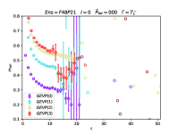
Lattice energy levels are extracted from the exponential decay of the principal correlators in Euclidean time.
We note in passing that due to exact isospin symmetry in our lattice calculation the channel is forbidden, but accounts only for about 2% of the decays in total.
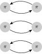
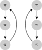
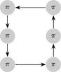
The number of quark contraction diagrams emerging in the construction of the relevant correlators grows factorially with the number of scattered particles. For instance, there are diagrams for when both sink and source are two-body operators, but in , with the topologies depicted in fig. 1. The remaining topologies can be found in section .2. Besides the complexity due to the large number of diagrams, most of the diagrams include disconnected quark annihilation sub-diagrams, which are difficult to calculate and induce a poor signal. Therefore, we employ the so-called distillation method [32] to compute all-to-all quark perambulators, and construct from these.
| Ensemble | Volume | ||
|---|---|---|---|
| F32P21 | |||
| F48P21 | |||
| F32P30 | |||
| F48P30 |


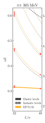
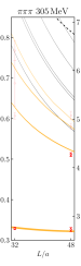
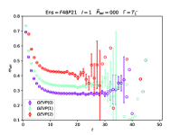
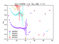
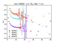
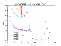
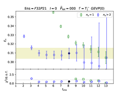
The resulting and finite-volume spectra are shown in fig. 2, with two volumes for each pion mass. The red dots, black dashed and black dot-dashed curves show the extracted energy levels, elastic non-interacting levels (corresponding to the and free energies), and the inelastic non-interacting levels, respectively. The ground levels appear in both and channels below the first non-interacting levels indicating strong attraction in the and channels. In the channel, at , the ground states are higher than threshold, indicating a resonance with non-zero phase space to decay; at , the ground levels are consistent for two volumes and are lower than the threshold, indicating a bound state. The orange bands represent predictions from the two- and three-body infinite-volume analysis using the EFT4 method introduced below.


Quantization conditions and resonance parameter— The finite-volume spectra discussed above contain two- and three-particle dynamics to be decoded through appropriate quantization conditions. In this work, we utilize the so-called Finite-Volume Unitarity (FVU) approach [23], which was already applied several times to a variety of three-body systems [13, 33, 18, 34, 20, 35, 36]. In the following we sketch the basics of this formalism while referring for more details to the given references.
The dominant interaction channel of the -system is formalized through the channel in the relative P-wave [24]. Thus, in the FVU formalism, the three-body finite-volume spectrum is predicted in the center-of-mass frame as a set of three-body energies for which
| (1) |
in the plane-wave/helicity (PWH) basis while projecting each element of this equation to the irrep of the group, see [37, 20]. The matrices (one-pion-exchange) and (self-energy of the -system in finite-volume) collect all on-shell configurations of the three pions and, therefore, single out all power-law volume dependence of this system. Together with the kinematical factor these matrices are entirely fixed. Contrary to this, the matrices and are volume-independent quantities (up to the neglected terms) containing information on the two- and three-body dynamics (or more loosely speaking force), respectively. The two-body force provides access to the two-body energy eigenvalues through which is equivalent to the usual Lüscher method [38] up to exponentially suppressed terms. While, in general, and are not known, various choices relevant for the and systems, relying on a generic parameterization and effective field theory are discussed below.
Generic method (GEN): the two-body force is parameterized as for the two-body invariant mass and a spectator momentum . We found that is entirely sufficient to describe the available lattice input, and this is also mathematically equivalent to the usual Breit-Wigner form. Similarly, the three-body force is parameterized through a general expansion in the JLS basis ( in relative P-wave) and then mapped to the PWH the standard techniques [39, 40, 36]. Here again, the order of the expansion depends on the availability/precision of the input. In the current case a two-parameter fit turned out as sufficiently flexible.
Effective field theory (EFT): The GEN methodology has an important drawback, not allowing for chiral extrapolation to the physical point. This can be circumvented through the use of the effective field theories as widely used in the two-body sector [22, 41] but not yet for study of three-hadron resonances from the lattice. Still, continuum results on and exist since several decades, see the review [25]. Using the results quoted in that review we perform a matching on the level of and scattering amplitudes. A somewhat lengthy but straightforward calculation at the tree-level yields
| (2) |
where the latter is expressed in the JLS basis, projected to the PWH basis [39, 40, 36]. Throughout this derivation, we have assumed that two- and three-pion interactions are saturated by the -channel resonance exchange (justified by the narrow width of the - and -mesons) and set following Ref. [25]. Thus far, the matching relations eq. 2 provide access to the two- and three-body force given three unknown parameters (). The KSFR relation [42, 43] allows one to reduce this set further by stating that . Indeed, this specifies already a chiral () extrapolation through the from chiral perturbation theory [44]. Furthermore, using the generalized KSFR relation () only one parameter is required to simultaneously describe and systems, we refer to this scenario as EFT1. Allowing, however, for a pion-mass independent shift defines the EFT2 method referring to free parameters . Finally, abandoning the KSFR relation entirely we define the EFT4 method by [45] and , leaving us with four free parameters . Clearly, one has to see the proposed EFT methods as representatives of a larger class of effective field theories with heavy degrees of freedom [3]. Ultimately, the defined method will be tested with respect to the lattice QCD results.
Finally, the three-body parameters obtained through a fit to the lattice spectra will be used to obtain the universal parameters of the - and -mesons through their pole positions on the second Riemann sheet. The necessary framework is provided through the Infinite-Volume Unitarity (IVU) approach [46, 23] corresponding to the above quantization conditions. Specifically, the part of the scattering amplitude relevant to the emergence of resonance poles is obtained through an integral equation
| (3) |
where we have suppressed energy, the helicity, and momenta arguments for brevity, see also eq. 1 and Refs. [20, 47, 36]. Here, denotes the usual self-energy integral. The above integral equation can be solved by standard techniques [48, 40, 36] projecting it first to the JLS basis and solving the integral equation through the complex contour deformation. Subsequently, complex pole positions can be extracted as shown in Refs. [20, 47, 35]. The corresponding procedure for finding two-body resonance poles simply boils down to finding solutions on the second Riemann sheet.
Before coming to the main results, we note that the three-body quantization condition is necessarily formulated as a determinant equation for infinitely dimensional matrices (PWH basis). This is a genuine feature of all three-body formalisms [22] reflected also in the fact that the determined three-body force depends on the momentum cutoff. Throughout, the following study we assume all momenta up to for computational reasons. Related to this is also the fact that for smaller volumes the spectator momentum cutoff leads to negative values of the two-body invariant mass. Since the exact form of the is not known in this (unphysical) region we cut it off with a simple form-factor replacing . We have tested other functional forms and values of and , finding no relevant effect on the extracted observables. For further details on cutoff effects in the context of three-body systems see Refs. [13, 40, 36].
Results and discussion— For each ensemble, the two-body finite-volume spectra consist of three energy eigenvalues located below the first inelastic threshold considering that two pions need to have one unit of momentum for the . In the three-body spectra, we restrict ourselves to the analysis of the ground states and the first excited state for larger-volume ensembles as shown in fig. 2. While qualitatively also higher levels seem to be predicted well enough by the approach, their quantitative study requires both an enlargement of the set of lattice operators as well as an update of the formalism including more free parameters due to the close proximity of the next excited state of the -meson, the .
With respect to these data, the method GEN yields best fits with including cross-correlations. For more details of the fit results and the obtained parameters, see section .4. Global (generalized KSFR) EFT1 method does not converge to a reasonable minimum and is neglected henceforth. Global EFT2 fits yields . Provided the precision level of our data, it is noticeable that also the EFT2 model is excessively rigid. Furthermore and as discussed below, the corresponding pole positions extrapolated to the physical point exhibit discrepancies with the empirical data. In contrast to this, the EFT4 fit provides a much better description of the finite-volume spectrum for , which are, indeed, quite close to the phenomenological values [49, 3]. In the following, we consider EFT4 as our main result, with GEN and EFT2 results providing a measure for systematic uncertainties. In principle, EFT4 could be improved by including further chiral corrections, but this goes beyond the scope of this work.

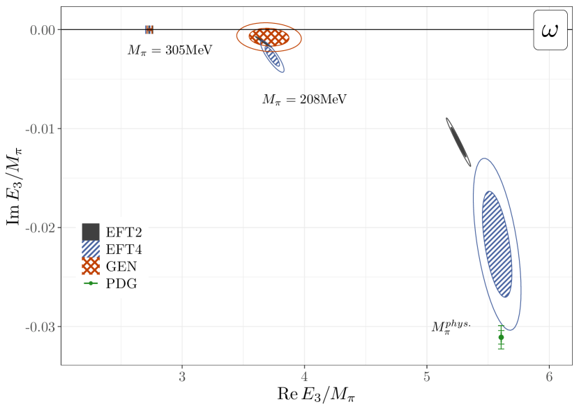
The results on the and pole positions using the IVU formalism eq. 3 with respect to the three discussed methods are shown in fig. 3. In both cases and for each pion mass, we observe agreement between all three methods regarding the real part of the pole position, while the determined imaginary part agrees on the level of . For the heavier pion mass value, the -meson is indeed a bound state with a binding energy of around . We note that the GEN results for the have to be taken with a grain of salt since for each pion mass only two volumes are available for the channel, each of which provides only one data point in the energy region close to the expected mass. Thus, a residual mass/width dependence in these results can be expected. Because EFT results connect different pion masses this is not an issue there. Instead, we observe that the EFT2 pole positions are narrowed to a very small region provided that only one parameter contains all the information on the -meson. The corresponding error ellipses are slightly larger due to the presence of the second parameter . Finally, the EFT4 agrees much better with the lattice results on the level of the finite-volume spectra as well as the corresponding GEN pole positions. Extrapolated to the physical pion mass it agrees astonishingly well () with the phenomenological and masses [50] and within also with their widths. The numerical results in physical units read
| (4) | |||||
| (5) |
implying for instance also an mass difference of , which agrees surprisingly well with the result obtained in Ref. [56]. The small deviation from the empirical value could be mitigated by taking into account the fact that in some cases too small volumes (see table 1) could give non-negligible exponential effects and discretization errors.
Conclusions— In this letter, we have reported the first-ever lattice QCD estimates of the -meson mass and width. One challenge in this calculation consists in particular in the precise estimation of finite-volume spectra from lattice QCD. In resolving the complete low-lying spectrum of states, multi-hadron operators prove to be essential [57]. The three-particle operators we use (see section .1) require a significant computational effort to compute all the relevant fermion contractions, a task which has only recently become feasible due to advances in algorithms, methods, and computational power. Another challenge concerns the development of the appropriate formalism to not only map the finite-volume results to the infinite-volume transition amplitudes but to also establish a reliable connection to the pertinent effective field theories, allowing us to perform the so far unprecedented chiral extrapolation of three-body resonance parameters to the physical point. The final results show a good agreement of this theoretical multi-step procedure with the empirical values [50] regarding the mass of both - and -mesons. The width turns out slightly smaller than the experimental value, but still agrees within uncertainties.
The presented study marks a new milestone in hadron spectroscopy from lattice QCD, paving the way toward understanding more complex systems. For closer to physical pion mass lattice setups the kinematic window to study resonance properties shrinks due to the proximity of the next inelastic thresholds (e.g., ). Thus, it may be advantageous to use more stable and widely available results at unphysical pion mass values and extrapolate to the physical point by making use of robust effective field theory methodology. In many successful investigations of resonant two-body systems this is already standard, but the corresponding treatment of resonant three-body systems has not yet been available. Future steps include the assessment of discretization errors as well as the inclusion of further volumes to reduce the uncertainties further. Applications towards the Roper-resonance and in an extension of the current methodology are also intriguing to investigate.
Acknowledgments— We thank the CLQCD collaborations for providing us the gauge configurations with dynamical fermions [26], which are generated on the HPC Cluster of ITP-CAS, the Southern Nuclear Science Computing Center(SNSC), the Siyuan-1 cluster supported by the Center for High Performance Computing at Shanghai Jiao Tong University and the Dongjiang Yuan Intelligent Computing Center.
HY is grateful to members of CLQCD for helpful discussions. Software QUDA [58, 59, 60] is used to solve the perambulators, as performed in Ref. [61]. HY acknowledges support from NSFC under Grant No. 12293060, 12293061, 12293063, and 11935017. This project was funded by the Deutsche Forschungsgemeinschaft (DFG,
German Research Foundation) as part of the CRC 1639 NuMeriQS – project no. 511713970 and by the MKW NRW under the funding code NW21-024-A. MM thanks M. Döring, D. Sadasivan, H. Akdag and P. C. Bruns for useful discussions.
This work is supported by the Deutsche Forschungsgemeinschaft (DFG, German Research Foundation) through the Sino-German Collaborative Research Center CRC110 “Symmetries and the Emergence of Structure in QCD” (DFG Project ID 196253076 - TRR 110). The work of MM was further supported through the Heisenberg Programme (project number: 532635001). The work of UGM was supported in part by the CAS President’s International Fellowship Initiative (PIFI) (Grant No. 2025PD0022). Part of the simulations were performed on the High-performance Computing Platform of Peking University, the QBiG GPU cluster at HISKP/Univ. Bonn, the Southern Nuclear Science Computing Center (SNSC), and the supercomputing system in the Dongjiang Yuan Intelligent Computing Center.
References
- Sakurai [1960] J. J. Sakurai, Theory of strong interactions, Annals Phys. 11, 1 (1960).
- Feynman [1973] R. P. Feynman, Photon-hadron interactions (1973).
- Meißner et al. [1986] U.-G. Meißner, N. Kaiser, A. Wirzba, and W. Weise, Skyrmions With and Mesons as Dynamical Gauge Bosons, Phys. Rev. Lett. 57, 1676 (1986).
- Kaiser and Weise [2024] N. Kaiser and W. Weise, Sizes of the nucleon, Phys. Rev. C 110, 015202 (2024), arXiv:2404.11292 [nucl-th] .
- Erkelenz [1974] K. Erkelenz, Current status of the relativistic two nucleon one boson exchange potential, Phys. Rept. 13, 191 (1974).
- Brown and Jackson [1976] G. Brown and A. Jackson, The nucleon-nucleon interaction (North-Holland, Amsterdam, 1976).
- Barkov et al. [1985] L. M. Barkov et al., Electromagnetic Pion Form-Factor in the Timelike Region, Nucl. Phys. B 256, 365 (1985).
- O’Connell et al. [1997] H. B. O’Connell, B. C. Pearce, A. W. Thomas, and A. G. Williams, mixing, vector meson dominance and the pion form-factor, Prog. Part. Nucl. Phys. 39, 201 (1997), arXiv:hep-ph/9501251 .
- McNeile et al. [2022] C. McNeile et al. (Fermilab Lattice, HPQCD, MILC), Progress report on computing the disconnected QCD and the QCD plus QED hadronic contributions to the muon’s anomalous magnetic moment., PoS LATTICE2021, 039 (2022), arXiv:2112.11339 [hep-lat] .
- Hippert et al. [2022] M. Hippert, J. Setford, H. Tan, D. Curtin, J. Noronha-Hostler, and N. Yunes, Mirror neutron stars, Phys. Rev. D 106, 035025 (2022), arXiv:2103.01965 [astro-ph.HE] .
- Hippert et al. [2023] M. Hippert, E. Dillingham, H. Tan, D. Curtin, J. Noronha-Hostler, and N. Yunes, Dark matter or regular matter in neutron stars? How to tell the difference from the coalescence of compact objects, Phys. Rev. D 107, 115028 (2023), arXiv:2211.08590 [astro-ph.HE] .
- Mai et al. [2023] M. Mai, U.-G. Meißner, and C. Urbach, Towards a theory of hadron resonances, Phys. Rept. 1001, 1 (2023), arXiv:2206.01477 [hep-ph] .
- Mai and Döring [2019] M. Mai and M. Döring, Finite-Volume Spectrum of and Systems, Phys. Rev. Lett. 122, 062503 (2019), arXiv:1807.04746 [hep-lat] .
- Blanton et al. [2020] T. D. Blanton, F. Romero-López, and S. R. Sharpe, Three-Pion Scattering Amplitude from Lattice QCD, Phys. Rev. Lett. 124, 032001 (2020), arXiv:1909.02973 [hep-lat] .
- Culver et al. [2020] C. Culver, M. Mai, R. Brett, A. Alexandru, and M. Döring, Three pion spectrum in the channel from lattice QCD, Phys. Rev. D 101, 114507 (2020), arXiv:1911.09047 [hep-lat] .
- Hansen et al. [2021] M. T. Hansen, R. A. Briceño, R. G. Edwards, C. E. Thomas, and D. J. Wilson (Hadron Spectrum), Energy-Dependent Scattering Amplitude from QCD, Phys. Rev. Lett. 126, 012001 (2021), arXiv:2009.04931 [hep-lat] .
- Fischer et al. [2021] M. Fischer, B. Kostrzewa, L. Liu, F. Romero-López, M. Ueding, and C. Urbach, Scattering of two and three physical pions at maximal isospin from lattice QCD, Eur. Phys. J. C 81, 436 (2021), arXiv:2008.03035 [hep-lat] .
- Alexandru et al. [2020] A. Alexandru, R. Brett, C. Culver, M. Döring, D. Guo, F. X. Lee, and M. Mai, Finite-volume energy spectrum of the system, Phys. Rev. D 102, 114523 (2020), arXiv:2009.12358 [hep-lat] .
- Draper et al. [2023] Z. T. Draper, A. D. Hanlon, B. Hörz, C. Morningstar, F. Romero-López, and S. R. Sharpe, Interactions of K, K and KK systems at maximal isospin from lattice QCD, JHEP 05, 137, arXiv:2302.13587 [hep-lat] .
- Mai et al. [2021a] M. Mai, A. Alexandru, R. Brett, C. Culver, M. Döring, F. X. Lee, and D. Sadasivan (GWQCD), Three-Body Dynamics of the a1(1260) Resonance from Lattice QCD, Phys. Rev. Lett. 127, 222001 (2021a), arXiv:2107.03973 [hep-lat] .
- Hansen and Sharpe [2019] M. T. Hansen and S. R. Sharpe, Lattice QCD and Three-particle Decays of Resonances, Ann. Rev. Nucl. Part. Sci. 69, 65 (2019), arXiv:1901.00483 [hep-lat] .
- Mai et al. [2021b] M. Mai, M. Döring, and A. Rusetsky, Multi-particle systems on the lattice and chiral extrapolations: a brief review, Eur. Phys. J. ST 230, 1623 (2021b), arXiv:2103.00577 [hep-lat] .
- Mai and Döring [2017] M. Mai and M. Döring, Three-body Unitarity in the Finite Volume, Eur. Phys. J. A 53, 240 (2017), arXiv:1709.08222 [hep-lat] .
- Gell-Mann et al. [1962] M. Gell-Mann, D. Sharp, and W. G. Wagner, Decay rates of neutral mesons, Phys. Rev. Lett. 8, 261 (1962).
- Meißner [1988] U.-G. Meißner, Low-Energy Hadron Physics from Effective Chiral Lagrangians with Vector Mesons, Phys. Rept. 161, 213 (1988).
- Hu et al. [2024] Z.-C. Hu, B.-L. Hu, J.-H. Wang, M. Gong, G. Liu, L. Liu, P. Sun, W. Sun, W. Wang, Y.-B. Yang, and D.-J. Zhao (CLQCD Collaboration), Quark masses and low-energy constants in the continuum from the tadpole-improved clover ensembles, Phys. Rev. D 109, 054507 (2024).
- Yan [2024] H. Yan, Operator construction (OpTion), in preparation (2024).
- Michael and Teasdale [1983] C. Michael and I. Teasdale, Extracting Glueball Masses From Lattice QCD, Nucl. Phys. B 215, 433 (1983).
- Luscher and Wolff [1990] M. Luscher and U. Wolff, How to Calculate the Elastic Scattering Matrix in Two-dimensional Quantum Field Theories by Numerical Simulation, Nucl. Phys. B 339, 222 (1990).
- Blossier et al. [2009] B. Blossier, M. Della Morte, G. von Hippel, T. Mendes, and R. Sommer, On the generalized eigenvalue method for energies and matrix elements in lattice field theory, JHEP 04, 094, arXiv:0902.1265 [hep-lat] .
- Fischer et al. [2020] M. Fischer, B. Kostrzewa, J. Ostmeyer, K. Ottnad, M. Ueding, and C. Urbach, On the generalised eigenvalue method and its relation to Prony and generalised pencil of function methods, Eur. Phys. J. A 56, 206 (2020), arXiv:2004.10472 [hep-lat] .
- Peardon et al. [2009] M. Peardon, J. Bulava, J. Foley, C. Morningstar, J. Dudek, R. G. Edwards, B. Joó, H.-W. Lin, D. G. Richards, and K. J. Juge (Hadron Spectrum Collaboration), Novel quark-field creation operator construction for hadronic physics in lattice qcd, Phys. Rev. D 80, 054506 (2009).
- Mai et al. [2020] M. Mai, M. Döring, C. Culver, and A. Alexandru, Three-body unitarity versus finite-volume spectrum from lattice QCD, Phys. Rev. D 101, 054510 (2020), arXiv:1909.05749 [hep-lat] .
- Brett et al. [2021] R. Brett, C. Culver, M. Mai, A. Alexandru, M. Döring, and F. X. Lee, Three-body interactions from the finite-volume QCD spectrum, Phys. Rev. D 104, 014501 (2021), arXiv:2101.06144 [hep-lat] .
- Garofalo et al. [2023] M. Garofalo, M. Mai, F. Romero-López, A. Rusetsky, and C. Urbach, Three-body resonances in the 4 theory, JHEP 02, 252, arXiv:2211.05605 [hep-lat] .
- Feng et al. [2024] Y. Feng, F. Gil, M. Döring, R. Molina, M. Mai, V. Shastry, and A. Szczepaniak, A unitary coupled-channel three-body amplitude with pions and kaons, (2024), arXiv:2407.08721 [nucl-th] .
- Göckeler et al. [2012] M. Göckeler, R. Horsley, M. Lage, U.-G. Meißner, P. E. L. Rakow, A. Rusetsky, G. Schierholz, and J. M. Zanotti, Scattering phases for meson and baryon resonances on general moving-frame lattices, Phys. Rev. D 86, 094513 (2012), arXiv:1206.4141 [hep-lat] .
- Lüscher [1991] M. Lüscher, Two particle states on a torus and their relation to the scattering matrix, Nucl. Phys. B 354, 531 (1991).
- Chung [1971] S. U. Chung, SPIN FORMALISMS 10.5170/CERN-1971-008 (1971).
- Sadasivan et al. [2020] D. Sadasivan, M. Mai, H. Akdag, and M. Döring, Dalitz plots and lineshape of from a relativistic three-body unitary approach, Phys. Rev. D 101, 094018 (2020), [Erratum: Phys.Rev.D 103, 019901 (2021)], arXiv:2002.12431 [nucl-th] .
- Mai et al. [2019] M. Mai, C. Culver, A. Alexandru, M. Döring, and F. X. Lee, Cross-channel study of pion scattering from lattice QCD, Phys. Rev. D 100, 114514 (2019), arXiv:1908.01847 [hep-lat] .
- Riazuddin and Fayyazuddin [1966] Riazuddin and Fayyazuddin, Algebra of current components and decay widths of rho and K* mesons, Phys. Rev. 147, 1071 (1966).
- Kawarabayashi and Suzuki [1966] K. Kawarabayashi and M. Suzuki, Partially conserved axial vector current and the decays of vector mesons, Phys. Rev. Lett. 16, 255 (1966).
- Gasser and Leutwyler [1984] J. Gasser and H. Leutwyler, Chiral Perturbation Theory to One Loop, Annals Phys. 158, 142 (1984).
- Bruns and Meißner [2005] P. C. Bruns and U.-G. Meißner, Infrared regularization for spin-1 fields, Eur. Phys. J. C 40, 97 (2005), arXiv:hep-ph/0411223 .
- Mai et al. [2017] M. Mai, B. Hu, M. Döring, A. Pilloni, and A. Szczepaniak, Three-body Unitarity with Isobars Revisited, Eur. Phys. J. A 53, 177 (2017), arXiv:1706.06118 [nucl-th] .
- Sadasivan et al. [2022] D. Sadasivan, A. Alexandru, H. Akdag, F. Amorim, R. Brett, C. Culver, M. Döring, F. X. Lee, and M. Mai, Pole position of the a1(1260) resonance in a three-body unitary framework, Phys. Rev. D 105, 054020 (2022), arXiv:2112.03355 [hep-ph] .
- Hetherington and Schick [1965] J. H. Hetherington and L. H. Schick, Exact Multiple-Scattering Analysis of Low-Energy Elastic K–d Scattering with Separable Potentials, Phys. Rev. 137, B935 (1965).
- Dax et al. [2018] M. Dax, T. Isken, and B. Kubis, Quark-mass dependence in decays, Eur. Phys. J. C 78, 859 (2018), arXiv:1808.08957 [hep-ph] .
- Workman et al. [2022] R. L. Workman et al. (Particle Data Group), Review of Particle Physics, PTEP 2022, 083C01 (2022).
- Akhmetshin et al. [2004] R. R. Akhmetshin et al. (CMD-2), Reanalysis of hadronic cross-section measurements at CMD-2, Phys. Lett. B 578, 285 (2004), arXiv:hep-ex/0308008 .
- Achasov et al. [2003] M. N. Achasov et al., Study of the process in the energy region below 0.98 GeV, Phys. Rev. D 68, 052006 (2003), arXiv:hep-ex/0305049 .
- Garcia-Martin et al. [2011] R. Garcia-Martin, R. Kaminski, J. R. Pelaez, and J. Ruiz de Elvira, Precise determination of the f0(600) and f0(980) pole parameters from a dispersive data analysis, Phys. Rev. Lett. 107, 072001 (2011), arXiv:1107.1635 [hep-ph] .
- Pelaez [2004] J. R. Pelaez, Light scalars as tetraquarks or two-meson states from large and unitarized chiral perturbation theory, Mod. Phys. Lett. A 19, 2879 (2004), arXiv:hep-ph/0411107 .
- Colangelo et al. [2001] G. Colangelo, J. Gasser, and H. Leutwyler, scattering, Nucl. Phys. B 603, 125 (2001), arXiv:hep-ph/0103088 .
- McNeile et al. [2009] C. McNeile, C. Michael, and C. Urbach (ETM), The omega-rho meson mass splitting and mixing from lattice QCD, Phys. Lett. B 674, 286 (2009), arXiv:0902.3897 [hep-lat] .
- Wilson et al. [2015] D. J. Wilson, R. A. Briceno, J. J. Dudek, R. G. Edwards, and C. E. Thomas, Coupled scattering in -wave and the resonance from lattice QCD, Phys. Rev. D 92, 094502 (2015), arXiv:1507.02599 [hep-ph] .
- Clark et al. [2010] M. Clark, R. Babich, K. Barros, R. Brower, and C. Rebbi, Solving lattice qcd systems of equations using mixed precision solvers on gpus, Computer Physics Communications 181, 1517 (2010).
- Babich et al. [2011] R. Babich, M. A. Clark, B. Joó, G. Shi, R. C. Brower, and S. Gottlieb, Scaling lattice qcd beyond 100 gpus, in Proceedings of 2011 International Conference for High Performance Computing, Networking, Storage and Analysis, SC ’11 (2011).
- Clark et al. [2016] M. A. Clark, B. Joó, A. Strelchenko, M. Cheng, A. Gambhir, and R. C. Brower, Accelerating lattice qcd multigrid on gpus using fine-grained parallelization, in Proceedings of the International Conference for High Performance Computing, Networking, Storage and Analysis, SC ’16 (2016).
- Yan et al. [2024] H. Yan, C. Liu, L. Liu, Y. Meng, and H. Xing, (2024), arXiv:2404.13479 [hep-lat] .
Supplemental Material
.1 Table of operators
Each operator used in this work is a linear combination of quark bilinear or the product of bilinears. First, we construct the operators in the flavor space. Let , etc. For channel, the following flavor structure is used:
| (S1) |
where and are one-body and two-body operators, respectively.
For channel, the following structure of bilinears is designed to enforce the isoscalar projection
| (S2) |
The operator set includes all one-, two-, and three-body operators to overlap with the dynamical channels in this study.
Second, the two-body operators are further projected onto the irrep in the momentum space to detect the P-wave. With OpTion [27], the explicit forms of the operators are printed. For convenience, the operators are represented as
| (S3) |
and are uniquely identified by the parameters , and . is the Cartesian gamma matrices and corresponds to . is the momenta for each meson. For convenience, the parameters are denoted by
| (S4) |
where one-to-one corresponds to the momentum vector. One direction notation in means one unit of momentum in that direction. For example, , , etc. The space projection coefficients are shown in Tab. 1.
| channel | type | operator |
| one | ||
| two | ||
| one | ||
| two | ||
| three |
Non-local operators with covariant derivatives are tested. The resulting spectra do not lead to noticeable change and as a result, this kind of operators are disposed out of the operator set.
.2 Topologies of the contraction diagrams
After projecting to isospin , only certain topologies remain. The topologies of are illustrated in the main text. The schematics of other diagrams including the three-pion operators, i.e., and , are shown in Fig. S1.


Topologies in the two-pion and one-pion sectors are shown in Fig S2. The type of topologies is the same as those for scattering, with one of the replaced by the meson and the target resonance replaced by the .


.3 Spectra
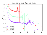
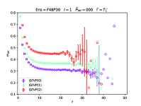
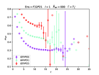
In this section, we present the details of extracting finite-volume energy levels from the correlation matrices . To determine the lowest levels, we solve the GEVP for each ensemble,
| (S5) |
where are the eigenvalues corresponding to the eigenvectors . For the channel, we use matrices and for the channel, we use matrices using the operators in table 1. The choice of the reference time has negligible impact on the resulting spectra.
The effective mass of the eigenvalues in the and channel are shown in Figs. S3 and S3, respectively. The plots exhibit plateaus at large . The thermal pollution in the channel is eliminated by shifting the correlation matrices before solving GEVP. The thermal pollution in the channel is not evident with the current precision, and is, thus, ignored in the analysis.
The energy levels of the excited states are extracted by doing a two-state fit of :
| (S6) |
where is the energy level.
We inspected the dependence of the levels on the fitting range and chose the starting point such that the fit yields a reasonable and remains stable against changes in the fitting range. An example of this stability analysis for the ground state in the channel of ensemble F32P21 is shown in fig. S5. Statistical uncertainties are estimated from Bootstrap samples.
.4 Fit results
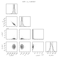
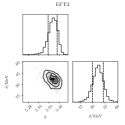
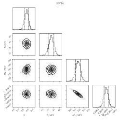
Details of the fit results for the GEN(305), GEN(208), EFT2(208/305) and EFT4(208/305) methods of parametrizing two- and three-body force. All values are estimated for the spectator momentum cutoff and left-hand cutoff form-factor . Statistical uncertainties are estimated from Bootstrap samples. The distribution and covariances of the parameters of GEN and EFT fits are shown in the corner plots fig. S6 and fig. S7, respectively.
| Parameters | ||||
| 305 | ||||
| 208 | ||||
| 305/208 | ||||