Regenerative Ulam-von Neumann Algorithm: An Innovative Markov chain Monte Carlo Method for Matrix Inversion

Abstract

This paper presents an extension of the classical Ulan-von Neumann Markov chain Monte Carlo algorithm for the computation of the matrix inverse. The algorithm presented in this paper, termed as regenerative Ulam-von Neumann algorithm, utilizes the regenerative structure of classical, non-truncated Neumann series defined by a non-singular matrix and produces an unbiased estimator of the matrix inverse. Furthermore, the accuracy of the proposed algorithm depends on a single parameter that controls the total number of Markov transitions simulated thus avoiding the challenge of balancing between the total number of Markov chain replications and its corresponding length as in the classical Ulam-von Neumann algorithm. To efficiently utilize the Markov chain transition samples in the calculation of the regenerative quantities, the proposed algorithm quantifies automatically the contribution of each Markov transition to all regenerative quantities by a carefully designed updating scheme that utilized three separate matrices containing the current weights, total weights, and regenerative cycle count, respectively. A probabilistic analysis of the performance of the algorithm, including the variance of the estimator, is provided. Finally, numerical experiments verify the qualitative effectiveness of the proposed scheme.

68Q25, 68R10, 65C05

1 Introduction

Markov chain Monte Carlo (MCMC) methods is an important class of algorithms that draw sample paths from a Markov chain. One well-known application of MCMC is the numerical solution of linear systems, also known as the Ulam-von Neumann algorithm due to its original application in thermonuclear dynamics computations by Stanisław Ulam and John von Neumann [16]. The main idea behind the Ulam-von Neumann algorithm lies in constructing and sampling a discrete Markov chain with a state space defined by the rows of the iteration matrix and a carefully designed transition probability matrix [5, 19]. Monte-Carlo-type methods can be appealing on a variety of applications due to high parallel granularity and and ability to compute partial solutions of systems of linear equations [35]. Thus, various Monte-Carlo algorithms have been suggested for the solution of linear systems, e.g., see [35, 27, 24, 5, 33, 7] for an non-exhaustive list.

In this paper we consider the related problem of computing an approximation of the inverse of a non-singular $d\times d$ matrix $A$ via MCMC [33, 12, 4, 25, 18, 13, 28]. A straightforward implementation of the Ulam-von Neumann algorithm samples the Markov chain to estimate a truncation of the Neumann series $(I-A)^{-1}=\sum_{n=0}^{\infty}A^{n}$. For a finite-state Markov chain with transition matrix $P$, $[P^{n}]_{ij}$, the $(i,j)$-th element of the $n$-th power of $P$, represents the probability of the Markov chain transits from the state $i$ to state $j$ after $n$ steps. Meanwhile, this probability can be estimated by Monte-Carlo simulations of the Markov chain, therefore, these simulations can be used to estimate the powers of the matrix, hence the inverse via the Neumann series; more recent development are summarized in [1, 17, 19, 12]. The accuracy of such algorithm primarily depends on the total number of paths of the Markov chain as well as and the truncation threshold (length) of each independent path. For different type of matrices, it is observed that interactions of these two factors can have significant impact on the quality of the algorithm, see, e.g., [30].

The algorithm presented in this paper, termed as regenerative Ulam-von Neumann algorithm, utilizes the regenerative structure of the Neumann series defined by a non-singular matrix and produces an unbiased estimator of the inversion, i.e., we estimate the non-truncated series. We then provide a probabilistic analysis of the quality of the algorithm. More specifically, the second moment of the samples is quantified through two independent central limit theorems, one for Markov chains on symmetric groups and one for the summation of weakly dependent random variables. A list of contribution of this paper is as follows:

• Algorithm: upon observing a regenerative structure in running the classic Ulam-von Neumann algorithm, we identify a stochastic fixed point equation (3) that is induced by the regenerative structure. This observation allows us to introduce an alternative estimator for MCMC matrix inversion in the form of the regenerative quantities $\alpha^{ij},i,j\in[d]$, which are also solutions to the stochastic fixed point equation. This new estimator does not require any forms of truncation of the Neumann series, hence it is an unbiased estimator. Furthermore, the accuracy of the algorithm only depends on one parameter, the total number of Markov transitions simulated, avoiding the challenge of balancing between two different factors, as in the classical Ulam-von Neumann algorithm. To efficiently utilize the Markov chain transition samples in the calculation of the regenerative quantities, we design and implement an algorithm (Algorithm 1) that quantifies the contribution of each Markov transition to all regenerative quantities via exploiting three separate matrices that contain current weights, total weights, and regenerative cycle count, respectively.

• Analysis: to quantify the variance of the estimator -and thus the quality of the algorithm- a central limit theorem (CLT) described in Theorem 4.1 is established. There are two key components in proving Theorem 4.1. First, we present a connection between the evolution of the counting matrix $\Gamma$ and a Markov chain on the symmetric group, thus obtain a CLT, Theorem 4.10, as a consequence of extensive research in the area of Markov chains on finite groups. Second, we obtain a CLT, Theorem 4.12, for the cumulative weight matrix $\Sigma$, as a direct result of a general Lindberg CLT for weakly dependent random vectors, Theorem 4.16, whose proof follows basic approaches in the literature but offers more precise and straightforward estimations.

• Applications: we illustrate the qualitative performance of the proposed algorithm on both sparse and dense matrices. The proposed algorithm can be also applied on scientific applications where the entries of the matrix inverse are required, e.g., data uncertainty quantification [21], and Katz centrality [26, 24].

1.1 Organization and notation

Section 2 summarizes related previous work, and in particular the Ulam-von Neumann algorithm for matrix inversion. Section 3 presents our main algorithmic contribution that exploits the regenerative structure of Ulam-Von Neumann. In Section 4, probabilistic analysis of the algorithm, including the central limit theorems for estimating the variance of our estimator, is presented. Applications and numerical experiments are presented in Section 5. Finally, our concluding remarks are presented in Section 6.

The $ij$-th entry of the matrix $A$ is denoted by $A_{ij}$ while the $ij$-th entry of the matrix power $A^{k},\ k\in\mathbb{Z}$, is denoted by $[A^{k}]_{ij}$. The term $\mathbb{E}[\cdot]$ denotes the expectation operator. The spectral radius of the matrix $A$ is equal to the maximum of the absolute values of its eigenvalues and will be denoted by $\rho(A)$. The symbol ${\bf 1}_{d}$ denotes the $d\times 1$ vector of all ones while on certain occasions we write $[d]$ to represent the interval $[1,2\ldots,d]$. Finally, the variable $\mathbbm{1}_{[\alpha=\beta]}$ is equal to one when $\alpha$ is equal to $\beta$, and zero otherwise.

2 Markov chain Monte-Carlo (MCMC) matrix inversion (Ulam-von Neumann algorithm)

Consider a $d\times d$ matrix $B=I-A$ where $\rho(A)<1$. The matrix $B$ is non-singular and its inverse matrix can be represented via the Neumann series

$$B^{-1}=\sum_{k=0}^{\infty}A^{k}.$$

Let us denote $C=B^{-1}=(I-A)^{-1}$, and ${\cal X}$, an aperiodic and irreducible Markov chain associated with the $d\times d$ transition probability matrix $P$ where $P_{ij}$ denotes the transition probability from state $i$ to state $j$. The entries of the matrix $P$ can be set in different ways as long as the sum of the entries of its rows and columns is at most equal to one [5]. For example, a possible choice is to set the entries of the matrix $P$ as $P_{ij}=\frac{|A_{ij}|}{\sum_{k=1}^{d}|A_{ik}|}$. Using the above notation, the problem of computing the matrix inverse $B^{-1}$ becomes equivalent to that of computing the entries $C_{ij},\ i,j\in[d]$ of the matrix $C$. In the following we describe the Ulam-von Neumann algorithm to compute $C_{ij}$ for any index pair $(i,j)\in[d]\times[d]$.

Remark 1.

To simplify notation, throughout the rest of this paper we consider the approximation of the matrix inverse $B^{-1}=(I-A)^{-1}$. Computing the matrix inverse $A^{-1}$ can be achieved by replacing $A$ with the linear transformation $P(A)=I-A$.

Let the current replicate of the Markov chain ${\cal X}$ be initiated at some state ${\cal X}_{r}(0)=i,\ 1\leq i\leq d$, for each replicate of the Markov chain indexed by $r$ and represented as ${\cal X}_{r}$. Furthermore, let $W^{r}_{0}=1$ be a fixed scalar, and define the following sequence of (scalar) random variables for $k>0$:

$$W^{r}_{k}=W^{r}_{k-1}\frac{A_{{\cal X}_{r}(k-1){\cal X}_{r}(k)}}{P_{{\cal X}_{r}(k-1){\cal X}_{r}(k)}},$$

where the random variable $W^{r}_{k}$ represents the likelihood ratio of the transition with respect to the probability induced by the Markov chain ${\cal X}_{r}$. The key idea of the Ulam-von Neumann algorithm is then based on the following simple observation.

Lemma 2.1.

For any initial state $1\leq i\leq d$, it holds that

$$\mathbb{E}\left[W_{k}^{r}\mathbbm{1}_{[{\cal X}_{r}(k)=j]}\right]=\left[A^{k}\right]_{ij},$$

i.e., the expectation of the random variable $W_{k}^{r}\mathbbm{1}_{[{\cal X}_{r}(k)=j]}$ is equal to the $(i,j)$-th element of $A^{k}$ for any $r=1,2,\ldots,R$, and $k\in\mathbb{N}$.

Proof 2.2.

This can be proved by induction. The case $k=0$ and $k=1$ are straightforward. For the general case where we update $W_{k}^{r}$ to $W_{k+1}^{n}$, we can write:

$$\mathbb{E}\left[W_{k+1}^{r}\mathbbm{1}_{[n_{k+1}=j]}\right]= \mathbb{E}[\mathbb{E}[W_{k+1}^{r}\mathbbm{1}_{[{\cal X}_{r}(k+1)=j]}|{\cal X}_{r}(k)]]$$

$$= \mathbb{E}\left[\mathbb{E}\left[W_{k}^{r}\frac{A_{{\cal X}_{r}(k),j}}{P_{{\cal X}_{r}(k),j}}\bigg{|}{\cal X}_{r}(k)\right]\right]$$

$$= \mathbb{E}\left[\mathbb{E}\left[\left[A^{k}\right]_{i,{\cal X}_{r}(k)}\frac{A_{{\cal X}_{r}(k),j}}{P_{{\cal X}_{r}(k),j}}\bigg{|}{\cal X}_{r}(k)\right]\right]$$

$$= \left[A^{k+1}\right]_{ij}.$$

Define now the following approximation of $C_{ij}$ after $R\in\mathbb{N}$ replications of the Markov chain ${\cal X}$, where each replication consists of $r_{k}$ transitions:

(1) $$\widehat{C}^{R}_{ij}:=\frac{1}{R}\sum_{r=1}^{R}\left[\sum_{k=0}^{r_{k}}W^{r}_{k}\mathbbm{1}_{[{\cal X}_{r}(k)=j]}\right].$$

Lemma 2.1 establishes that $W_{k}^{r}$ is an unbiased estimator of $\left[A^{k}\right]_{ij}$. Therefore, the sum $\sum_{k=0}^{r_{k}}W^{r}_{k}\mathbbm{1}_{[{\cal X}_{r}(k)=j]}$ approaches $C_{ij}$ in average as $r_{k}$ tends to infinity, and $\widehat{C}^{R}_{ij}$ can be viewed as a reasonable estimator of $C_{ij}$. A necessary and sufficient condition for the convergence of the Ulam-von Neumann algorithm is as follows.

Theorem 2.3 (Theorem 4.2 in [19]).

Given a $d\times d$ transition probability matrix $P$ and a non-singular matrix $B$ such that $\rho(B)<1$, the Ulam-von Neumann algorithm converges if and only if $\rho\left(\widehat{H}\right)<1$, where $\widehat{H}_{ij}=\begin{cases}\left[A^{2}\right]_{ij}/P_{ij}&\mathrm{if}\ P_{ij}\neq 0\\ 0&\mathrm{otherwise}.\end{cases}.$

The algorithm and analysis presented throughout the rest of this paper assume that the transition probability matrix $P$ satisfies the convergence criterion in Theorem 2.3.

3 Regenerative Ulam-von Neumann Algorithm: random walk and stochastic fixed point equation

In this section, we present a new implementation of the MCMC matrix inversion algorithm based on the regenerative structure of the discrete Markov chain ${\cal X}$ operating on states defined by the rows of the matrix $A$. In contrast to standard MCMC, our regenerative approach can compute an approximation of all entries of $B^{-1}$ while starting from any randomly initialized state $i\in[d]$. Moreover, only one such initialization is required since, for any particular state, the Markov chain ${\cal X}$ restarts itself every time the same state is observed and these non-overlapping segments of the Markov chain are independent. Thus we no longer need to pick values for the parameters controlling the number and length of the Markov chain replicas, as in classical MCMC.

3.1 The Basics of the Algorithm

Let us focus first on the main diagonal of the inverse matrix $C$, and in particular, the approximation of $C_{ii}$, for certain $i\in[d]$. For convenience we remind that classical MCMC sets $\widehat{C}_{ii}$ equal to the sample mean of the $R$ realizations of the random variable $\sum_{k=0}^{r_{k}}W_{k}\mathbbm{1}_{[{\cal X}(k)=i]}$ generated via the Markov chains ${\cal X}_{r},\ r=1,\ldots,R$, where each chain starts from the state $i$.

Instead of $R$ separate Markov chains, we now consider a single Markov chain ${\cal X}$ that starts at state $i\in[d]$. We let the Markov chain progress for an indeterminate number of steps while registering the portions of the chain that occur between returns to the state $i$. Since each such portion occurs independently of the other, the state $i$ is a regeneration point [32]. For any $k\in\mathbb{N}\cup\{0\}$ we define the initial state variable $\tau^{ii}_{0}=0$ followed by

$$\tau^{ii}_{k+1} =\inf\{t>\tau^{ii}_{k}|{\cal X}(t)=i\}.$$

The variable $\tau^{ii}_{k+1}$ denotes the $(k+1)$-th return to state $i$ (starting from the same state $i$) and thus the chain does not visit $i$ between $\tau^{ii}_{k}$ and $\tau^{ii}_{k+1}$. Following the above definition, we now write $W_{\tau^{ii}_{k+1}}=W_{\tau^{ii}_{k}}\cdot\alpha^{ii}_{n}$, where by the regenerativity of the Markov chain ${\cal X}$, the scalars $\alpha^{ii}_{n}$ are i.i.d. random variables counting the increment of $W_{k}$ between the $\tau^{ii}_{k}$ and $\tau^{k}_{k+1}$. More precisely, we can write

$$\alpha^{ii}_{k}=\prod_{\ell=\tau^{ii}_{k}}^{\tau^{ii}_{k+1}-1}\frac{a_{n_{\ell}{n_{\ell+1}}}}{p_{n_{\ell}{n_{\ell+1}}}}.$$

Thus, setting $W_{0}=1$, we can rewrite

(2) $$Z_{ii}:=\sum_{k=0}^{\infty}W_{k}\mathbbm{1}_{[{\cal X}(k)=i]} =\sum_{n=0}^{\infty}W_{\tau_{n}}=W_{0}\sum_{n=0}^{\infty}\prod_{k=1}^{n}\alpha^{ii}_{k}.$$

Let the symbol $\stackrel{{\scriptstyle d}}{{=}}$ imply that the left-hand side and right-hand side of an equation have the same probability distribution. The expression in (2) solves the following stochastic fixed point equation:

(3) $$Z_{ii}\stackrel{{\scriptstyle d}}{{=}}W_{0}+\alpha^{ii}Z_{ii},$$

where $\alpha^{ii}$ and $Z_{ii}$ are assumed to be independent, $\alpha^{ii}$ denotes the distribution of $\alpha^{ii}_{n},\ n>0$, and $Z_{ii}$ denotes the distribution of $\sum_{n=0}^{\infty}W_{\tau^{ii}_{n}}$.

Remark 3.1.

Stochastic fixed point equations have deep connections to Lyapunov exponent and random matrix theory. Recently, applications have been found in heavy tail phenomenon in stochastic gradient descent. Detailed studies on stochastic fixed point equations can be found in [29, 8].

Taking expectations on both sides in (3) implies that

$$\mathbb{E}[Z_{ii}]=\dfrac{1}{1-\mathbb{E}[\alpha^{ii}]}.$$

Thus, an estimate of $\mathbb{E}[\alpha^{ii}]$ leads to that of the quantity $C_{ii}=\mathbb{E}[Z_{ii}]$. Note that while there might be multiple solutions to the stochastic fixed-point equation (3), the important aspect here is that they should all -in expectation- point to the same relationship. Furthermore, the second moment is equal to

$$\mathbb{E}[Z^{2}_{ii}]=1+2\mathbb{E}[\alpha^{ii}]\mathbb{E}[Z_{ii}]+\mathbb{E}[(\alpha^{ii})^{2}]\mathbb{E}[Z^{2}_{ii}],$$

and thus

$$\mathbb{E}[Z^{2}_{ii}]=\frac{1+\mathbb{E}[\alpha^{ii}]}{(1-\mathbb{E}[\alpha^{ii}])(1-\mathbb{E}[(\alpha^{ii})^{2}])}.$$

For the off-diagonal terms $Z_{ij},i\neq j$, once again consider the starting point $i$ of the Markov chain ${\cal X}$ and define $\tau_{ij}=\inf\{t>0,|X(t)=j\}$ and $\alpha^{ij}=\prod_{\ell=0}^{\tau^{ij}-1}\frac{a_{n_{\ell}{n_{\ell+1}}}}{p_{n_{\ell}{n_{\ell+1}}}}$. Then, we have

$$Z_{ij} :=\sum_{k=0}^{\infty}W_{k}\mathbbm{1}_{[{\cal X}(k)=j]}\stackrel{{\scriptstyle d}}{{=}}\sum_{n=0}^{\infty}\alpha^{ij}\prod_{k=1}^{n}\alpha_{k}^{jj}=\alpha^{ij}Z_{jj}.$$

Moreover, $\alpha^{ij}$ and $Z_{jj}$ are independent in the last term. Hence, $C_{ij}=\mathbb{E}[\alpha^{ij}]C_{ii}$.

3.2 Implementation of the Algorithm

The key to the implementation of the regenerative algorithm is to accurately record the involved (cumulative) weights and the accounting of the regenerative structure. To keep track of of the running weights, cumulative weights and counting of the regenerative cycles (in other words the disjoint segments of the chain), we introduce three $d\times d$ matrices, $\Lambda$, $\Sigma$, and $\Gamma$, respectively. The cycles are identified by a starting state and ending state, which forms the indices of the three matrices. Once the chain is initialized at some random state $i\in[d]$, the algorithm iterates until $\min_{q,l}\Gamma_{q,l}\geq N$. Here, the only parameter $N\in\mathbb{N}$ controls the variance of the estimator, see Theorem 4.1. The proposed regenerative Ulam-von Neumann Algorithm is summarized in Algorithm 1.

The running weights matrix $\Lambda$ keeps track of the weights during the regenerative cycle. When the chain reaches state $i$, all cycles starting at state $i$ are re-initiated and the elements of the $i$th row of $[\Lambda]_{i}$ that are equal to zero (corresponding to previous cycles that were closed) are reset to one. As the chain arrives at the following state $j$, the entries of the matrix $\Lambda$ are scaled by $\frac{A_{ij}}{P_{ij}}$ and all cycles that terminate at index $j$ close while the information from the $j$th column of the matrix $\Lambda$ is transferred (added) to the respective column of the cumulative weights $\Sigma$. Finally, the $j$th column of the matrix $\Lambda$ is reset to zero. In order to keep the count of the number of cycles in the chain, the $j$th column of the matrix $\Gamma$ increases by one. The loop continues until the count of the performed cycles is large enough, i.e., larger than an input parameter $N$. Note that the updating the $j$th column of $\Lambda$ by zero at the end and by one at the start of the cycle assures that the segments are disjoint and therefore independent.

1

Input : $A\in\mathbb{R}^{d\times d},\ P\in\mathbb{R}^{d\times d}$, and scalar $N\in\mathbb{N}$. Also define and set the matrices $\Lambda\in\mathbb{R}^{d\times d},\ \Sigma\in\mathbb{R}^{d\times d},\ \Gamma\in\mathbb{N}^{d\times d}$ equal to zero.

2 Initialization: Initialize the Markov chain at some random state $i\in[d]$.

3 while $\min_{q,l}\Gamma_{q,l}<N$ do

4         Update the $i$-th row of $\Lambda$: $\Lambda_{ik}=\Lambda_{ik}+\mathbbm{1}_{[\Lambda_{ik}=0]}$, for all $k=1,2,\ldots,d$;

5       Progress the Markov chain to state $j$.

6       Update $\Lambda$: $\Lambda=\Lambda\times\frac{A_{ij}}{P_{ij}}$;

7       Update $j$-th column of $\Gamma$: $\Gamma_{kj}=\Gamma_{kj}+1$ if $\Lambda_{kj}\neq 0$, for all $k=1,2,\ldots,d$;

8       Update $j$-th column of $\Sigma$: $\Sigma_{kj}=\Sigma_{kj}+\Lambda_{kj}$, for all $k=1,2,\ldots,d$;

9       Reset the $j$-th column of $\Lambda$: $\Lambda_{kj}=0$ for all $k=1,2,\ldots,d$;

10       Over-write $i\leftarrow j$.

11 end while

Output : 

$$\widehat{C}_{ij}=\left\{\begin{array}[]{cc}\dfrac{1}{1-\dfrac{\Sigma_{jj}}{\Gamma_{jj}}}&\mathrm{if}\ \ i=j\\ \\ \dfrac{\Sigma_{ij}}{\Gamma_{ij}}\dfrac{1}{1-\dfrac{\Sigma_{jj}}{\Gamma_{jj}}}&\mathrm{if}\ \ i\neq j.\end{array}\right.$$

12

Algorithm 1 Regenerative Ulam-von Neumann Algorithm

4 Probabilistic Analysis of Algorithm 1

The analysis in Section 3 established that the regenerative estimator is unbiased. To complete the analysis of algorithm, we establish the second order properties of the algorithm with a CLT-type of result, in the same spirit of output analysis elaborated in [34].

Denote $N$ as the number of Markov chain transitions that have been sampled, let $\left(\Sigma^{N},\Gamma^{N}\right)$ be the output matrices from the algorithm after these $N$ samples. Law of large number tell us that,

(4) $$\lim_{N\rightarrow\infty}\frac{\gamma^{N}_{ii}}{\gamma^{N}_{ii}-\sigma_{ii}^{N}}=C_{ii},\quad\lim_{N\rightarrow\infty}\frac{\sigma_{ij}^{N}}{\gamma^{N}_{ij}}\frac{\gamma^{N}_{jj}}{\gamma^{N}_{jj}-\sigma_{jj}^{N}}=C_{ij},\quad\forall i,j\in[d]\,.$$

Theorem 4.1.

Given a $d\times d$ matrix $A$, a Markov chain on the stat space of the rows of $A$ with transition matrix $(P_{ij})$, there exists a $d\times d$ symmetric and positive semi-definite matrix $\Sigma_{C}$, such that $\sqrt{N}\frac{\sigma_{ij}^{N}}{\gamma^{N}_{ij}}-C_{ij}$ converge to a $n^{2}$-variate normal variable with covariance matrix $\Sigma_{C}$, as $N\rightarrow\infty$.

Proof 4.2.

As demonstrated in Theorem 2.1 of [22], the theorem is the consequence of the central limit theorems established in Theorems 4.10 and 4.12, with a properly defined function that reflects the relationship between the state of the regenerative process and the estimated quantities depicted in (4).

4.1 Central Limit Theorem for $\Gamma$ Matrix

In this section, we focus on the growth of the $\Gamma$ matrix in Algorithm 1, key to the accuracy of the algorithm, as we will see later. First, let us consider an alternative algorithm, Algorithm 2, that calculates only the $\Gamma$ matrix.

1

Input : $d\times d$ matrices, $\Pi=\Gamma=0$.

2 Pick initial $i$, while $\min_{i,j}\gamma_{i,j}<N$ do

3      Update the $i$-th row of $\Pi$: $\pi_{ik}=1$, for all $k=1,\ldots,d$

4       Pick $j$

5       Update $j$-th column of $\Gamma$: $\gamma_{\cdot,j}=\gamma_{\cdot,j}+\pi_{\cdot,j}$

6       Reset the $j$-th column of $\Pi$: $\pi_{\cdot,j}=0$.

7       Over-write $i\leftarrow j$.

8 end while

9

Output : $\Gamma$

10

Algorithm 2 The Calculation of $\Gamma$ Matrix

We summarize the following result in a Lemma but omit its proof since it is straightforward.

Lemma 4.3.

Algorithm 2 produces an identical $\Gamma$ matrix as Algorithm 1 for the same pseudo-random number sequence.

Matrices $\Pi$ produced by Algorithm 2 are binary. A careful examine of its evolution reveals that the possibility of $0-1$ matrices that $\Pi$ takes is significantly less than the total number of $2^{d^{2}}$.

First, the operation in the algorithm can be formalized by the following operator, $k\in[d]$,

$$(T_{k},\Pi)_{ij}=\left\{\begin{array}[]{cc}0&j=k,i\neq k,\\ 1&i=k,\\ \pi_{ij}&\hbox{otherwise.}\end{array}.\right.$$

Note that $T_{k}$ only changes the values in the $k$-th row and $k$-th column and that the relations $\pi_{ik}+\pi_{ki}=1$ for $i\neq k$ and $\pi_{kk}=1$ are invariant under each $T_{k}$. After an initial phase when each $T_{k}$ has been invoked at least once, the elements of the matrix $\Pi$ will satisfy the invariant relations $\pi_{ij}+\pi_{ji}=1$ for all $i\neq j$ and $\pi_{ii}=1$ for all $i\in[d]$. Let us term this initial phase as warming up phase. By the irreducibility and aperiodic assumption of the Markov chain $X(t)$, as stated in the beginning of Section 3, we know that the warming up phase will be finished almost surely. Afterwards, $\Pi$ will always satisfy these invariant relations.

A few important observations help us narrow down the amount of possible matrices and furnish them with structural properties.

Lemma 4.4.

Let $T^{p}_{J}:=T_{j_{p}}\circ\ldots\circ T_{j_{2}}\circ T_{j_{1}}$ with $J:=(j_{p},\ldots,j_{1})\in[d]^{p}$ and any $i\in[d]$ we have $T_{i}\circ T^{p}_{J}\circ T_{i}\,\Pi=T_{i}\circ T^{p}_{J}\,\Pi$.

Proof 4.5.

It can be seen easily that $\pi_{ij}=1$ and $\pi_{ji}=0$ for $j\neq i$ for both $T_{i}\circ T^{p}_{J}\circ T_{i}\,\Pi$ and $T_{i}\circ T^{p}_{J}\,\Pi$. All the other values are determined solely by $\Pi$ and $T^{p}_{J}$.

Lemma 4.4 implies that for a long sequence of $T_{k}$ operations, repetitions can be simplified to the last operation applied. More precisely, for $T^{m}_{N}=T_{n_{m}}\circ\dots\circ T_{n_{1}}$, with $N=(n_{m},\ldots,n_{1})\in[d]^{m}$, let the set of distinct $n_{i}$’s have the cardinality $m^{*}\leq m$ and the sequence $N^{*}=(n^{*}_{m^{*}},\dots,n^{*}_{1})$ consists of all the distinct $n_{j}$’s in the order as they first appearance from left to right in $N$, $n^{*}_{m^{*}}=n_{m}$ and $n^{*}_{k}=n_{\ell}$, $\ell=\inf\left\{k:n_{k}\notin\{n^{*}_{m^{*}},\ldots,n^{*}_{k+1}\}\right\}$. Let $T^{m^{*}}_{N^{*}}=T_{n^{*}_{m^{*}}}\circ\ldots\circ T_{n_{1}^{*}}$. We have,

$$T^{m}_{N}\Pi =T^{m^{*}}_{N^{*}}\Pi\qquad\text{ that is }$$

$$T_{n_{m}}\circ\dots\circ T_{n_{1}}\Pi =T_{n_{m^{*}}^{*}}\circ\ldots\circ T_{n_{1}^{*}}\Pi\,.$$

The ordered sequence, $n^{*}_{m^{*}},\ldots n^{*}_{1}$ can be viewed naturally as a part of a permutation on $[n]$. Indeed, we also have,

Lemma 4.6.

For any permutation $\sigma$ of $[d]$, let $T^{d}_{\sigma}=T_{\sigma(d)}\circ T_{\sigma(d-1)}\circ\cdots T_{\sigma(2)}\circ T_{\sigma(1)}$ Then for any $0-1$ matrices $\Pi$ and $\Pi^{\prime}$, $T^{d}_{\sigma}\Pi=T^{d}_{\sigma}\Pi^{\prime}\,.$

Proof 4.7.

It can be verified that the end results of either side do not depend on the initial matrix.

Therefore, after the warming up phase, the matrix $\Pi$ is completely determined by the permutation corresponding to the last $n$ distinct $T_{k}$ applied to the initial matrix. We stress that after the warm up phase the image of the starting matrix depends only on the last permutation and is independent on the starting matrix.

There exists a bijection, denoted by $K_{d}$ from $S_{d}$ the set of all the permutation to $P_{d}$ the set of the matrices that we get after the warming up phase, there are $d!$ possible distinct matrices after the warm up. This allows us to denote these matrices by $\Pi_{\sigma}$ with $\sigma$ being the permutation it corresponds to.

Define $(\Pi_{0})_{ij}=\delta_{i\geq j}$, that is

$$\Pi_{0}:=\left(\begin{array}[]{cccccc}1&0&0&\ldots&0&0\\ 1&1&0&\ldots&0&0\\ 1&1&1&\ldots&0&0\\ &&&\ldots&&\\ 1&1&1&\ldots&1&0\\ 1&1&1&\ldots&1&1\end{array}\right)\,.$$

Then, it is straightforward to verify the following lemma.

Lemma 4.8.

$T_{n}\circ T_{n-1}\circ\ldots\circ T_{2}\circ T_{1}\,M=\Pi_{0}$, for any $0-1$ matrix $M$.

Thus, in this bijection the permutation $\sigma=(1,2,\ldots d)$, which is the identity in the symmetric group $S_{d}$ maps any $M$ to $\Pi_{0}\in P_{d}$, in particular $\sigma P_{d}=\{\Pi_{0}\}$.

If at time $t$, the Markov chain $X_{t}=i$ and suppose that $\Pi=\Pi_{\sigma_{t}}$. We have $X(t+1)=j$ with probability $p_{ij}$. This induces a map $\hat{T}$ on $S_{d}$ by

$$\sigma_{t+1}=\hat{T}(\sigma_{t})=({\hat{T}}_{j}\sigma_{t},j)$$

where, when $j$ is in the position $\ell+1$ in the permutation $\sigma_{t}$, $j=\sigma(\ell+1)$, and:

$${\hat{T}}_{j}(\sigma(1),\ldots\sigma(\ell),j,\sigma(\ell+2),\ldots\sigma(d))=(\sigma(1),\ldots\sigma(\ell),\sigma(\ell+2),\ldots\sigma(d)).$$

This is basically a Random-to-Bottom Shuffling Markov chain in the jargon of random walk on finite groups (see e.g. [31]), denoted by $Y(t)$. To see the reason for such term, consider a deck of $n$ indexed cards, and at each time, an index $j$ is determined with probability $p_{ij}$ where $i$ is the index of the card at the bottom, then the card with index $j$ will be moved to the bottom. The permutations produced by this procedure coincide with that produced by $Y_{t}$.

Lemma 4.9.

If $X(t)$ is a irreducible and aperiodic Markov chain with state space $[d]$, $Y(t)$ is a irreducible and aperiodic Markov chain with state space $S_{d}$.

Theorem 4.10.

Under the assumption of Theorem 4.1, there exists a $d\times d$ symmetric and positive semi-definite matrix $\Sigma_{s}$, such that the quantity $\sqrt{N}\left(\frac{\Gamma^{N}}{N}-\Sigma_{s}\right)$ converges to a $n^{2}$-variate normal variable with covariance matrix $\Sigma_{s}$, as $N\to\infty$.

Proof 4.11.

As we demonstrated before, after an initial phase, the increment of the $\Gamma$ matrix corresponding to randomly selecting among $n$ matrices, according to the state the sampling Markov chain is in. Suppose that $Z_{n}$ is a be a Harris ergodic Markov chain on a general state space ${\bf X}$ with invariant probability distribution $\pi$. Suppose that $f:{\bf X}\rightarrow\mathbb{R}^{*}$ is a Borel function to a finite dimensional Euclidean space. Define ${\bar{f}}_{n}:=n^{-1}\sum_{i=1}^{n}f(X_{i})$ and $\mathbb{E}_{\pi}f:=\int_{\bf X}f(x)\pi(dx)$. It is know from [9] that if the $Z_{n}$ is geometrically ergodic and $\mathbb{E}_{\pi}\|f\|^{2+\delta}<\infty$ for some $\delta>0$, then $\sqrt{n}({\bar{f}}_{n}-\mathbb{E}_{\pi}f)$ converge to a Gaussian distribution with a covariance matrix $\Sigma_{f}$ as $n\rightarrow\infty$.

Given our Markov chain $Y_{n}$ on the symmetric group $S_{d}$, define the following function $f:S_{d}\rightarrow\{0,1\}^{d},\sigma\mapsto K_{d}(\sigma)_{\sigma(n)}$. $Y_{n}$ is of course geometrically ergodic since it is an irreducible and aperiodic Markov chain on a finite state space, and certainly $\|f\|\leq d$.

4.2 Central Limit Theorem for Matrix $\Sigma$

Theorem 4.12.

Under the assumption of Theorem 4.1, there exists a $d\times d$ symmetric and positive semi-definite matrix $\Sigma_{a}$, such that the quantity $\sqrt{N}\left(\frac{\Sigma^{N}}{N}-\Sigma_{a}\right)$ converges to a $n^{2}$-variate normal variable with covariance matrix $\Sigma_{a}$, as $N\to\infty$, with $\Sigma^{N}$ being the matrices of cumulative weights.

Proof 4.13.

This is the direct consequence of Theorem 4.16 and Lemma 4.20.

Remark 4.14.

Here, we encounter a dependent sequence, see, e.g. [14], [10], [36]. We could not find the exact results required for our purpose in the published literature,  [15] and [3] are probably closest related. Therefore, we include a detailed proof for completeness. While we follow the general idea of Lindeberg method and block techniques in the proofs of many CLT, including those in [15], detailed technical calculations that are critical to the vector structure are different from what appeared in the literature.

The following definition of weak dependence can be found in both [14] and [15].

Definition 4.15.

Process $(X_{n})_{n\in{\mathbb{Z}}}$ is said to be $({\epsilon_{r}}_{r\in{\mathbb{Z}}},\psi)$-weakly dependent for a sequence of real number $\epsilon_{r}\downarrow 0$ and a function $\psi:N^{2}\times(\mathbb{R}_{+})^{2}\rightarrow\mathbb{R}^{+}$ if for any $r\geq 0$ and $(u+v)$-tuples of integers $s_{1}\leq\ldots\leq s_{u}\leq s_{u}+r\leq t_{1}\leq\ldots t_{v}$, we have,

$$|\mbox{\sf Cov}(f(X_{s_{1}},\ldots,X_{s_{u}}),g(X_{t_{1}},\ldots,X_{t_{v}})|\leq\psi(u,v,\mbox{\sf Lip}f,\mbox{\sf Lip}g)\epsilon_{r}$$

where $f$ and $g$ are two real valued function satisfying $\|f\|_{\infty},\|g\|_{\infty}\leq 1$, and $\mbox{\sf Lip}f$ and $\mbox{\sf Lip}g$ are the Lipschtz constants of function $f$ and $g$, respectively.

More precisely, we have,

$$\mbox{\sf Lip}f:=\sup_{(x_{1},x_{2},\ldots,x_{u})\neq(y_{1},y_{2},\ldots,y_{u})}\frac{|f(x_{1},x_{2},\ldots,x_{u})-f(y_{1},y_{2},\ldots,y_{u})|}{\|x_{1}-y_{1}\|+\ldots+\|x_{u}-y_{u}\|}.$$

Theorem 4.16.

Assume $\mathbb{R}^{d}$ random vectors $(X_{n})_{n\in{\mathbb{Z}}}$ are stationary, $\mathbb{E}[X_{n}]=0$ and satisfy $\mathbb{E}\|X_{0}\|^{m}<\infty$ for $m>2$. Furthermore, $\{X_{n}\}$ is a $({\epsilon_{r}}_{r\in{\mathbb{Z}}},\psi)$-weakly dependent sequence with $\epsilon_{r}=O(r^{-\kappa})$ for $\kappa>(2m-3)/(m-2)$, then, ${\hat{X}}_{n}=\frac{1}{\sqrt{n}}\sum_{k=1}^{n}X_{k}$ converge in distribution to $N(0,\Sigma^{2})$ with $\Sigma^{2}=\sum_{k=0}^{\infty}\mbox{\sf Cov}(X_{0},X_{k})=\sum_{k=0}^{\infty}\mathbb{E}[X_{0}X_{k}^{T}]$.

Proof 4.17.

The key is two sequences of positive integers $p_{n}$ and $q_{n}$ with $q_{n}\rightarrow\infty$, $q_{n}=o(p_{n})$, and there exists $\beta\in(0,1)$, $p_{n}=O(n^{1-\beta})$ and $q_{n}^{(2m-3)/(m-2)}=O(n)$ as $n\rightarrow\infty$. That means, both $p_{n}$ and $q_{n}$ go to infinity but slower than $n$, moreover $q_{n}$ grows slower than $p_{n}$. Define $k_{n}=\left[\frac{n}{p_{n}+q_{n}}\right]$, with $[\cdot]$ denotes the Gauss bracket, and

$$Z_{n}= \frac{1}{\sqrt{n}}(U^{n}_{1}+\ldots+U^{n}_{k_{n}}),\quad U^{n}_{j}=\sum_{i\in B^{n}_{j}}X_{i},$$

$$B^{n}_{j}= ((p_{n}+q_{n})(j-1),(p_{n}+q_{n})(j-1)+p_{n}]\cap\mathbb{N}$$

$$C^{n}_{j}= ((p_{n}+q_{n})(j-1)+p+1,(p_{n}+q_{n})j]\cap\mathbb{N}$$

$$V^{n}_{j}= \sum_{i\in C^{n}_{j}}X_{i}.$$

It is easy to see that the distance between any two $B$ blocks ($B_{j}^{n}$ and $B_{k}^{n}$ when $j\neq k$) is at least $q_{n}$, and $C_{j}^{n}$ contains the integers between $B^{n}_{j}$ and $B^{n}_{j-1}$. Let

$${\tilde{Z}}_{n}= \frac{1}{\sqrt{n}}({\tilde{U}}^{n}_{1}+\ldots+{\tilde{U}}^{n}_{k_{n}}),$$

$$Y_{n}= \frac{1}{\sqrt{n}}({\tilde{V}}^{n}_{1}+\ldots+{\tilde{V}}^{n}_{k_{n}}),$$

with ${\tilde{U}}^{n}_{i}$ being independent random variables following the same distribution as $U^{n}_{i}$, and ${\tilde{V}}^{n}_{i}$ being independent Gaussian variables with the same first two moments as $U^{n}_{i}$. For a fixed $t\in\mathbb{R}^{d}$ in a compact set $\Omega$ containing the origin, define $f:\mathbb{R}^{d}\rightarrow\mathbb{C},x\mapsto\exp(it\cdot x)$. Then,

$$\mathbb{E}[f({\hat{X}}_{n})-f(\Sigma)]$$

$$= \mathbb{E}[f({\hat{X}}_{n})-f(Z_{n})+f(Z_{n})-f({\tilde{Z}}_{n})+f({\tilde{Z}}_{n})-f(Y_{n})+f(Y_{n})-f(\Sigma)]$$

$$= \underbrace{\mathbb{E}[f({\hat{X}}_{n})-f(Z_{n})]}_{I}+\underbrace{\mathbb{E}[f(Z_{n})-f({\tilde{Z}}_{n})]}_{II}+\underbrace{\mathbb{E}[f({\tilde{Z}}_{n})-f(Y_{n})]}_{III}+\underbrace{\mathbb{E}[f(Y_{n})-f(\Sigma)]}_{IV}.$$

with $\Sigma$ the square root of matrix $\Sigma^{2}$.

The method of estimating the above four quantities and showing that they converge to zero as $n\rightarrow\infty$ is known as the Bernstein block technique of the Lindeberg method. Terms $II$ and $III$ are known to be the main terms, and the other two terms are often referred to as the auxiliary terms.

Calculation of the term $I$

$$|I|= |\mathbb{E}[f({\hat{X}}_{n})-f(Z_{n})]|$$

$$\leq \sup_{x\in\mathbb{R}^{d}}\|Df(x)\|_{op}\mathbb{E}[\|{\hat{X}}_{n})-f(Z_{n})\|_{2}^{2}]$$ Taylor’s expansion

$$\leq d\|t||^{2}\mathbb{E}\bigg{\|}\frac{1}{\sqrt{n}}(V^{n}_{1}+\ldots+V^{n}_{k_{n}})\bigg{\|}_{2}^{2} f U_{n} Z_{n}$$ definition of , and

$$\leq \frac{2d\|t\|^{2}}{n}\left[\sum_{j=1}^{k_{n}}\sum_{i\in C_{j}^{n}}\bigg{\|}\sum_{\ell\geq i}\mathbb{E}[X_{i}X_{\ell}]\bigg{\|}\right]$$

$$\leq \frac{2d\|t\|^{2}}{n}(k_{n}q_{n}+p_{n})(\|\Sigma^{2}\|) \sum_{j=1}^{k_{n}}V^{n}_{j}$$ by the number of terms in

and summability of covariance.

From the assumptions on $p_{n}$, $q_{n}$ and $k_{n}$ follows that $|I|$ tends to zero as $n\rightarrow\infty$.

Calculation of the term $II$

The term $II$ will be controlled through the weak dependent condition. Note that the correlations are controlled by the Lipschitz constant and $\epsilon_{n}$. The $1/\sqrt{n}$ scaling gives the Lipschitz to be of that order.

$$II= \mathbb{E}[f(Z_{n})-f({\tilde{Z}}_{n})]\leq\sum_{j=1}^{k_{n}}|\mathbb{E}\Delta^{n}_{j}|$$ with

$$\Delta^{n}_{j}= f(W_{j}^{n}+x^{n}_{j})-f(W_{j}^{n}+{\tilde{x}}^{n}_{j}),$$

$$x^{n}_{j}= \frac{1}{\sqrt{n}}U^{n}_{j},\qquad{\tilde{x}}^{n}_{j}=\frac{1}{\sqrt{n}}{\tilde{U}}^{n}_{j}$$

$$W^{n}_{j}= \sum_{i<j}x^{n}_{i}+\sum_{i>j}{\tilde{x}}^{n}_{i}\,.$$

It can be verified that,

$$|\mathbb{E}\Delta^{n}_{j}|\leq\Bigg{|}\mbox{\sf Cov}\left(f\left(\sum_{i<j}x^{n}_{i}\right),f(x^{n}_{j})\right)\Bigg{|}.$$

By the assumption that $\{X_{n}\}$ is a $({\epsilon_{r}},\psi)$-weakly dependent sequence (${r\in{\mathbb{Z}}}$), we have $\mathbb{E}|\Delta^{n}_{j}|\leq Ck_{n}p_{n}\epsilon_{q_{n}}$. Thus the condition of $\{\epsilon_{r}\}$, $p_{n}$ and $q_{n}$ leads to the desired result.

Calculation of the term $III$

The term $III$ will be controlled via the moment assumption. Note that the difference between the two sets of variables starts from the third moments, which we can bound using the moment condition.

$$III= \mathbb{E}[f({\tilde{Z}}_{n})-f(Y_{n})]\leq\sum_{j=1}^{k_{n}}|\mathbb{E}{\tilde{\Delta}}^{n}_{j}|\qquad\text{with}$$

$${\tilde{\Delta}}^{n}_{j}= f({\tilde{W}}_{j}^{n}+{\tilde{x}}^{n}_{j})-f({\tilde{W}}_{j}^{n}+{\hat{x}}^{n}_{j}),\qquad{\hat{x}}^{n}_{j}=\frac{1}{\sqrt{n}}{\tilde{V}}^{n}_{j},\qquad{\tilde{W}}^{n}_{j}=\sum_{i<j}{\tilde{x}}^{n}_{i}+\sum_{i>j}{\hat{x}}^{n}_{i}.$$

Then, $|\mathbb{E}{\tilde{\Delta}}^{n}_{j}|=|\mathbb{E}f({\tilde{x}}^{n}_{i})-\mathbb{E}f({\hat{x}}^{n}_{i})|$. There exist $C>0$, such that, for all $x\in\mathbb{R}^{d}$ and $t\in\Omega\subset\mathbb{R}^{d}$, for and $\alpha$ such that $\beta(1+\delta/2)\leq 1+\alpha/2$,

$$\bigg{\|}f(x)-(1+it\cdot x-\frac{1}{2}x^{T}(tt^{T})x)]\bigg{\|}\leq C\|x\|_{2+\alpha}^{2+\alpha}.$$

Therefore, the moment condition has the term $III$ bounded by $Cn^{-1-\frac{\alpha}{2}}k_{n}^{1+\frac{\delta}{2}}$ according to Lemma 4.18, and it goes to zero as $n\rightarrow\infty$ due to the way $\alpha$ is selected.

Calculation of the term $IV$

For $IV$, recall that the independent Gaussian variables ${\tilde{V}}^{n}_{i}$ have the same first two moments as $U^{n}_{i}$, i.e. $\mathbb{E}[{\tilde{V}}_{i}]=0$, and $\mathbb{E}[{\tilde{V}}^{n}_{i}({\tilde{V}}^{n}_{i})^{T}]=\mathbb{E}[U^{n}_{i}(U^{n}_{i})^{T}]$ and are independent of index $i$, let us define, $\Sigma^{2}_{n,p}=\mathbb{E}[{\tilde{V}}^{n}_{i}({\tilde{V}}^{n}_{i})^{T}]/p_{n}$, and it can be easily verified that $\Sigma^{2}_{n,p}\rightarrow\Sigma^{2}$ as $n\rightarrow\infty$.

Lemma 4.18.

For i.i.d random variable $X_{i}$ with finite $2+\delta$ moment for some $\delta>0$, there exists $C>0$ independent of $X$, such that, for any integer $n>1$ and any $0<\alpha<\delta$, we have,

(5) $$\mathbb{E}\left[\bigg{\|}\sum_{i=1}^{n}X_{i}\bigg{\|}^{2+\alpha}\right]\leq Cn^{\frac{2+\delta}{2}}(\mathbb{E}[|X_{1}|^{2+\delta}]).$$

Proof 4.19.

First, we will consider $X_{i}$ are symmetric, then, we can see that, for any $\alpha\leq\delta$,

$$\mathbb{E}\left[\bigg{\|}\sum_{i=1}^{n}X_{i}\bigg{\|}^{2+\alpha}\right]= \mathbb{E}\left[\left(\sum_{i=1}^{n}X_{i}\right)^{2}\bigg{\|}\sum_{k=1}^{n}X_{k}\bigg{\|}^{\alpha}\right]$$

$$= \sum_{i=1}^{n}\mathbb{E}\left[X_{i}^{2}\bigg{\|}\sum_{j=1}^{n}X_{j}\bigg{\|}^{\alpha}\right]+\sum_{i,j=1}^{n}\mathbb{E}\left[X_{i}X_{j}\bigg{|}\sum X_{i}\bigg{\|}^{\alpha}\right]$$

$$= n\mathbb{E}\left[X_{1}^{2}\bigg{\|}\sum_{j=1}^{n}X_{j}\bigg{\|}^{\alpha}\right],$$

the last step follows from the symmetric and iid assumptions. For $\alpha<\delta$, Hölder’s inequality gives us,

$$\mathbb{E}\left[X_{1}^{2}\bigg{\|}\sum_{j=1}^{n}X_{j}\bigg{\|}^{\alpha}\right]\leq (\mathbb{E}[|X_{1}|^{2+\delta}])^{\frac{2}{2+\delta}}\left(\mathbb{E}\left[\bigg{\|}\sum_{j=1}^{n}X_{j}\bigg{\|}^{\frac{\alpha(2+\delta)}{\delta}}\right]\right)^{\frac{\delta}{2+\delta}}$$

$$\leq (\mathbb{E}[|X_{1}|^{2+\delta}])^{\frac{2}{2+\delta}}\left(\mathbb{E}\left[\bigg{\|}\sum_{j=1}^{n}X_{j}\bigg{\|}^{2+\alpha}\right]\right)^{\frac{\delta}{2+\delta}},$$

because $\frac{\alpha(2+\delta)}{\delta}<2+\alpha$. Therefore, we have,

$$\mathbb{E}\left[\bigg{\|}\sum_{i=1}^{n}X_{i}\bigg{\|}^{2+\alpha}\right] \leq n(\mathbb{E}[|X_{1}|^{2+\delta}])^{\frac{2}{2+\delta}}\left(\mathbb{E}\left[\bigg{\|}\sum_{j=1}^{n}X_{j}\bigg{\|}^{2+\alpha}\right]\right)^{\frac{\delta}{2+\delta}}$$ so

$$\left(\mathbb{E}\left[\bigg{\|}\sum_{j=1}^{n}X_{j}\bigg{\|}^{2+\alpha}\right]\right)^{\frac{2}{2+\delta}} \leq n(\mathbb{E}[|X_{1}|^{2+\delta}])^{\frac{2}{2+\delta}}$$ thus

$$\mathbb{E}\left[\bigg{\|}\sum_{j=1}^{n}X_{j}\bigg{\|}^{2+\alpha}\right] \leq n^{\frac{2+\delta}{2}}(\mathbb{E}[|X_{1}|^{2+\delta}])\,.$$

For general sequence, (5) is obtained though applying the Khintchine’s inequality to its Rademacher average, see e.g. [23].

Lemma 4.20.

For any fixed integer $n$ and any $(i,j)\neq(k,\ell)$, the correlation between $\alpha^{ij}_{n}$ and $\alpha^{k\ell}_{n+m}$ decays exponentially with respect to $m$ as $m$ increases.

Proof 4.21.

It is enough to show that the correlations between $\alpha^{ij}_{1}$ and $\alpha^{k\ell}_{m}$ decay exponentially with respect to $m$. To see this, we have,

$$\mbox{\sf Cov}(\alpha^{ij}_{1},\alpha^{k\ell}_{m})$$

$$= \mathbb{E}[\alpha^{ij}_{1}\alpha^{k\ell}_{m}]-\mathbb{E}[\alpha^{ij}_{1}]\mathbb{E}[\alpha^{k\ell}_{m}]$$

$$= \mathbb{E}[(\alpha^{ij}_{1}-\mathbb{E}[\alpha^{ij}_{1}])(\alpha^{k\ell}_{m}-\mathbb{E}[\alpha^{k\ell}_{m}])]$$

$$= \mathbb{E}[(\alpha^{ij}_{1}-\mathbb{E}[\alpha^{ij}_{1}])\mathbbm{1}\{\tau^{ij}_{1}\geq m\}(\alpha^{k\ell}_{m}-\mathbb{E}[\alpha^{k\ell}_{m}])]$$

$$\leq [\mathbb{E}[(\alpha^{ij}_{1}-\mathbb{E}[\alpha^{ij}_{1}])^{2}\mathbbm{1}\{\tau^{ij}_{1}\geq m\}]^{\frac{1}{2}}[\mathbb{E}(\alpha^{k\ell}_{m}-\mathbb{E}[\alpha^{k\ell}_{m}])^{2}]^{\frac{1}{2}}.$$

The exponential decay follows easily form the fact that $\alpha$ is uniformly bounded.

5 Numerical Illustration

Our numerical experiments are conducted in a Matlab environment (version R2023b), using 64-bit arithmetic, on a single core of a computing system equipped with an Apple M1 Max processor and 64 GB of system memory. While Monte-Carlo-type approaches are highly parallelizable, their sequential execution is known to quickly become prohibitive as the matrix dimension increases, e.g., see [5]. Therefore, in this section we restrict ourselves to small matrix problems. All results reported in this section represent sample averages over ten independent executions.

We begin by considering the application of Algorithm 1 on two matrix problems:

• Discretized Laplacian: We consider a second central difference (5-point) discretization of the Laplace operator $\Delta$ on the unit square $\Omega=[0,1]\times[0,1]$ using Dirichlet boundary conditions. In order to satisfy the condition $\rho\left(\widehat{H}\right)<1$, we divide each non-zero entry by a factor of ten.

• Model covariance: We consider the following model covariance matrix:

  $$A_{ij}=\begin{cases}1+\sqrt{i}&\mathrm{if}\ i==j\\ 1/|i-j|^{2}&\mathrm{if}\ i\neq j\end{cases},$$

  where the off-diagonal entries of $A$ decay away the main diagonal in order to simulate a decreasing correlation among the variables. Similarly to the previous case, in order to satisfy the condition $\rho\left(\widehat{H}\right)<1$, we now divide each non-zero entry by a factor three.

For both types of matrices we over-write the resulting matrix as $A=I-A$ so that $B^{-1}=A^{-1}$.

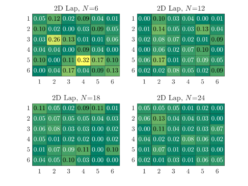
Figure 1: Entry-wise magnitude of the matrix $B^{-1}-\widehat{C}$ for the 5-point stencil discretization.

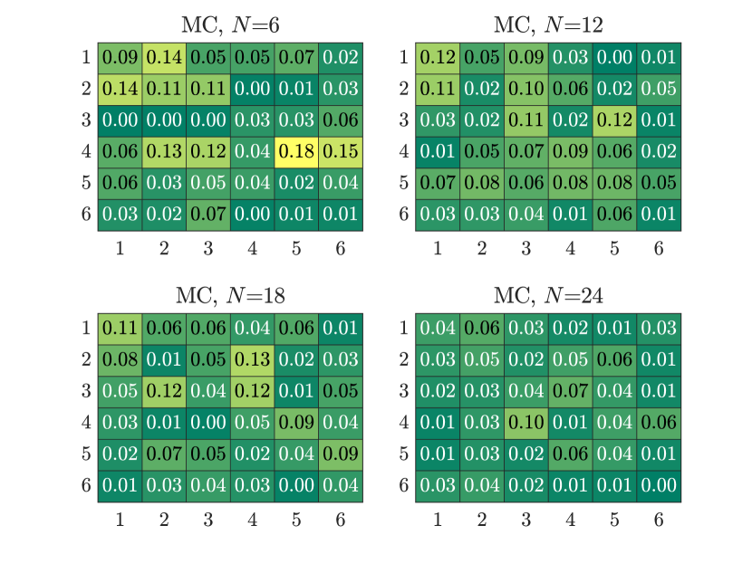
Figure 2: Entry-wise magnitude of the matrix $B^{-1}-\widehat{C}$ for the model covariance problem.

The termination of Algorithm 1 depends on the satisfaction of the condition $\min_{q,l}\Gamma_{q,l}<N$, and thus increasing $N$ allows the Markov chain to potentially run longer, leading to more regeneration points. Figures 1 and 2 plot the absolute error $B^{-1}_{ij}-\widehat{C}_{ij}$ for the 5-point stencil discretization of the Laplacian operator and model covariance matrix, respectively. For the sake of visualization, we set the dimension of each matrix equal to $d=6$ and vary the value of $N$ tested in the termination criterion $\min_{q,l}\Gamma_{q,l}<N$ of Algorithm 1. Since larger values of $N$ likely result to more steps, we expect a smaller absolute error as $N$ increases.

We now consider the relative approximation error between the matrix inverse $B^{-1}$ and its approximation $\widehat{C}$ on a set of slightly larger problems of size $d=128$. In particular, we consider two different metrics: $a)$ the Frobenius norm of the approximation of $B^{-1}$ by $\widehat{C}$ divided by the Frobenius norm of $B^{-1}$, i.e., $\|B^{-1}-\widehat{C}\|/\|B^{-1}\|$, and $b)$ the relative error in the approximation of the trace of $B^{-1}$ by the trace of $\widehat{C}$, i.e., $\mathrm{Tr}\left(B^{-1}-\widehat{C}\right)/\mathrm{Tr}\left(B^{-1}\right)$, where $\mathrm{Tr}\left(X\right)=\sum_{k=1}^{d}X_{kk}$. The trace of $\widehat{C}$ is computed by summing the $d$ individual diagonal entries and is a quantity of interest in data uncertainty quantification and other applications [20, 21]. Figure 3 plots the relative error in the approximation of $B^{-1}$ and $\mathrm{Tr}\left(B^{-1}\right)$ by $\widehat{C}$ (solid line) and $\mathrm{Tr}\left(C\right)$ (dashed line), respectively. Figure 4 plots a bar graph with the total number of iterations performed by Algorithm 1 as function of $N$.

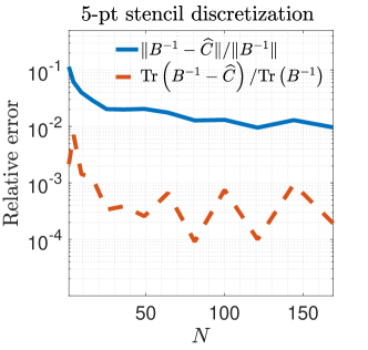
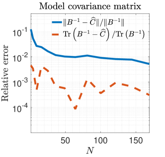
Figure 3: Solid curve: $\|B^{-1}-\widehat{C}\|/\|B^{-1}\|$. Dashed curve: $\mathrm{Tr}\left(B^{-1}-\widehat{C}\right)/\mathrm{Tr}\left(B^{-1}\right)$.

Finally, we consider the application of Algorithm 1 to determine Katz graph centrality, a centrality measure which extends the concept of eigenvector centrality by considering the influence of nodes that are connected through a path of intermediate nodes, i.e., beyond the immediate list of neighboring nodes [6]. Given a $d\times d$ adjacency matrix $A$, the Katz centrality of node $i$ equal to $x_{i}=\sum_{k=1}^{\infty}\alpha^{k}\sum_{j=1}^{d}A_{ij}x_{j}$ where the damping scalar $\alpha\in(0,1/\rho(A))$ controls the influence of the implicit walks. Gathering all centrality scores on a vector $x\in\mathbb{R}^{d}$, Katz centrality is equivalent to solving the sparse linear system $(I-\alpha A)x={\bf 1}_{d}$. For our example, we pick the IBM32 graph from the SuiteSparse matrix collection [11], a network from the original Harwell-Boeing sparse matrix test collection which represents leaflet interactions from a 1971 IBM advertisement conference. We set $\alpha=0.85/\|A\|_{2}$ and call Algorithm 1 to compute an approximation $\widehat{C}$ of $B^{-1}=(I-\alpha A)^{-1}$. Figure 5 plots the relative approximation error of the matrix inverse, as well as the error between the ideal Katz centrality $B^{-1}{\bf 1}_{d}$ and the approximation $\widehat{C}{\bf 1}_{d}$ (left subplot). As anticipated, increasing $N$ improves the quality of the matrix inverse approximation, which in turn leads to a higher number of correctly ranked nodes (right subplot).

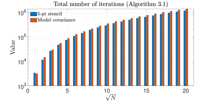
Figure 4: Total number of iterations performed by Algorithm 1 as a function of $N$.

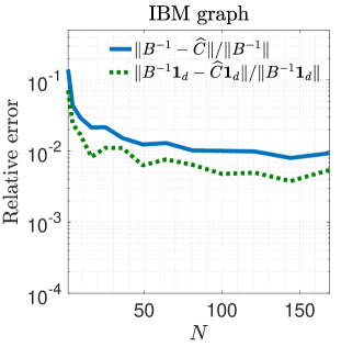
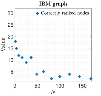
Figure 5: Left: plot of the quantities $\|B^{-1}-\widehat{C}\|/\|B^{-1}\|$ and $\|B^{-1}{\bf 1}_{d}-\widehat{C}{\bf 1}_{d}\|/\|B^{-1}{\bf 1}_{d}\|$. Right: number of correctly ranked nodes.

6 Conclusions

In this paper we presented and analyzed a Markov chain Monte Carlo algorithm to approximate the matrix inverse of a matrix. The proposed algorithm recasts the classical problem into one of a stochastic fixed point equation induced by the regenerative structure of the Markov chain. The associated proposed estimator does not require any truncation of the Neumann series and thus is unbiased. Moreover, only one parameter -the total number of simulated Markov transitions- is necessary, as opposed to the two parameters required in the Ulam-von Neumann algorithm. Numerical experiments verify that the proposed algorithm can indeed approximate all or a subset of the entries of the matrix inverse.

As part of our future work we plan to implement Algorithm 1 on shared memory high-performance computing architectures such as Graphics Processing Units (GPUs), and compare its performance against classical Markov chain Monte Carlo approaches. For example, in contrast to the algorithm of Ulam-von Neumann which relies on scalar multiplications, the main computation cost of Algorithm 1 stems from matrix-scalar multiplication of the form $\Lambda=\Lambda\times\frac{A_{ij}}{P_{ij}}$, an operation that can be parallelized quite efficiently on GPUs.

References

• [1] V. Alexandrov, Efficient parallel Monte Carlo methods for matrix computations, Mathematics and Computers in Simulation, 47 (1998), pp. 113–122.
• [2] S. Asmussen, Applied Probability and Queues, Springer, Second ed., 2003.
• [3] Bardet, Jean-Marc, Doukhan, Paul, Lang, Gabriel, and Ragache, Nicolas, Dependent lindeberg central limit theorem and some applications, ESAIM: PS, 12 (2008), pp. 154–172.
• [4] A. Barto and M. Duff, Monte Carlo matrix inversion and reinforcement learning, Advances in neural information processing systems, 6 (1993).
• [5] M. Benzi, T. M. Evans, S. P. Hamilton, M. Lupo Pasini, and S. R. Slattery, Analysis of Monte Carlo accelerated iterative methods for sparse linear systems, Numerical Linear Algebra with Applications, 24 (2017), p. e2088.
• [6] M. Benzi and C. Klymko, A matrix analysis of different centrality measures, arXiv preprint arXiv:1312.6722, (2014).
• [7] M. Benzi and M. Tuma, A parallel solver for large-scale Markov chains, Applied Numerical Mathematics, 41 (2002), pp. 135–153.
• [8] K. Burdzy, B. Kołodziejek, and T. Tadić, Stochastic fixed-point equation and local dependence measure, The Annals of Applied Probability, 32 (2022), pp. 2811 – 2840.
• [9] Chan, K. S. and Geyer, C. J., Comment on “Markov chains for exploring posterior distributions”, The Annals of Statistics, 22 (1994).
• [10] J. Chang, X. Chen, and M. Wu, Central limit theorems for high dimensional dependent data, Bernoulli, 30 (2024), pp. 712 – 742.
• [11] T. A. Davis and Y. Hu, The university of Florida sparse matrix collection, ACM Transactions on Mathematical Software (TOMS), 38 (2011), pp. 1–25.
• [12] I. Dimov, V. Alexandrov, and A. Karaivanova, Parallel resolvent Monte Carlo algorithms for linear algebra problems, Mathematics and Computers in Simulation, 55 (2001), pp. 25–35. The Second IMACS Seminar on Monte Carlo Methods.
• [13] I. Dimov, T. Dimov, and T. Gurov, A new iterative Monte Carlo approach for inverse matrix problem, Journal of Computational and Applied Mathematics, 92 (1998), pp. 15–35.
• [14] P. Doukhan and S. Louhichi, A new weak dependence condition and applications to moment inequalities, Stochastic Processes and their Applications, 84 (1999), pp. 313–342.
• [15] Doukhan, P. and Wintenberger,O., Invariance principle for new weakly dependent stationary models under sharp moment assumptions, Preprint, (2006).
• [16] S. Forsythe and R. Leibler, Matrix inversion by a Monte Carlo method, Math. Tables Other Aids Comput., 4 (1950), pp. 127–129.
• [17] V. N. A. G. M. MEGSON and I. T. DIMOV, Systolic matrix inversion using a Monte Carlo method, Parallel Algorithms and Applications, 3 (1994), pp. 311–330.
• [18] D. P. Heyman, Accurate computation of the fundamental matrix of a Markov chain, SIAM journal on matrix analysis and applications, 16 (1995), pp. 954–963.
• [19] H. Ji, M. Mascagni, and Y. Li, Convergence analysis of Markov chain Monte Carlo linear solvers using Ulam–von Neumann algorithm, SIAM Journal on Numerical Analysis, 51 (2013), pp. 2107–2122.
• [20] V. Kalantzis, C. Bekas, A. Curioni, and E. Gallopoulos, Accelerating data uncertainty quantification by solving linear systems with multiple right-hand sides, Numerical Algorithms, 4 (2013), pp. 637–653.
• [21] V. Kalantzis, A. C. I. Malossi, C. Bekas, A. Curioni, E. Gallopoulos, and Y. Saad, A scalable iterative dense linear system solver for multiple right-hand sides in data analytics, Parallel Computing, 74 (2018), pp. 136–153.
• [22] W. Kang, P. Shahabuddin, and W. Whitt, Exploiting regenerative structure to estimate finite time averages via simulation, ACM Trans. Model. Comput. Simul., 17 (2007), p. 8–es.
• [23] M. Ledoux and M. Talagrand, Probability in Banach Spaces: Isoperimetry and Processes, A Series of Modern Surveys in Mathematics Series, Springer, 1991.
• [24] F. Magalhães, J. Monteiro, J. A. Acebrón, and J. R. Herrero, A distributed Monte Carlo based linear algebra solver applied to the analysis of large complex networks, Future Generation Computer Systems, 127 (2022), pp. 320–330.
• [25] C. D. Meyer, Jr, The role of the group generalized inverse in the theory of finite Markov chains, SIAM Review, 17 (1975), pp. 443–464.
• [26] N. Guidotti, J. Acebrón, J. Monteiro, A Fast Monte Carlo algorithm for evaluating matrix functions with application in complex networks, in Journal of Scientific Computing, 99 (2024).
• [27] G. Ökten, Solving linear equations by Monte Carlo simulation, SIAM Journal on Scientific Computing, 27 (2005), pp. 511–531.
• [28] H. Prabhu, J. Rodrigues, O. Edfors, and F. Rusek, Approximative matrix inverse computations for very-large MIMO and applications to linear pre-coding systems, in 2013 IEEE Wireless Communications and Networking Conference (WCNC), IEEE, 2013, pp. 2710–2715.
• [29] U. Roesler, Stochastic fixed-point equations, Stochastic Models, 35 (2019), pp. 238–251.
• [30] E. Sahin, A. Lebedev, M. Abalenkovs, and V. Alexandrov, Usability of Markov chain Monte Carlo preconditioners in practical problems, in 2021 12th Workshop on Latest Advances in Scalable Algorithms for Large-Scale Systems (ScalA), 2021, pp. 44–49.
• [31] L. Saloff-Coste, Random Walks on Finite Groups, Springer Berlin Heidelberg, Berlin, Heidelberg, 2004, pp. 263–346.
• [32] W. L. Smith, Regenerative stochastic processes, Proceedings of the Royal Society of London. Series A. Mathematical and Physical Sciences, 232 (1955), pp. 6–31.
• [33] J. Straßburg and V. N. Alexandrov, A Monte Carlo approach to sparse approximate inverse matrix computations, Procedia Computer Science, 18 (2013), pp. 2307–2316.
• [34] D. Vats, J. M. Flegal, and G. L. Jones, Multivariate output analysis for Markov chain Monte Carlo, Biometrika, 106 (2019), pp. 321–337.
• [35] T. Wu and D. F. Gleich, Multiway Monte Carlo method for linear systems, SIAM Journal on Scientific Computing, 41 (2019), pp. A3449–A3475.
• [36] D. Zhang and W. B. Wu, Gaussian approximation for high dimensional time series, The Annals of Statistics, 45 (2017), pp. 1895 – 1919.