Energy-information trade-off makes the cortical critical power law the optimal coding
Abstract
Stimulus responses of cortical neurons exhibit the critical power law, where the covariance eigenspectrum follows the power law with the exponent just at the edge of differentiability of the neural manifold. This criticality is conjectured to balance the expressivity and robustness of neural codes, because a non-differential fractal manifold spoils coding reliability. However, contrary to the conjecture, here we prove that the neural coding is not degraded even on the non-differentiable fractal manifold, where the coding is extremely sensitive to perturbations. Rather, we show that the trade-off between energetic cost and information always makes this critical power-law response the optimal neural coding. Direct construction of a maximum likelihood decoder of the power-law coding validates the theoretical prediction. By revealing the non-trivial nature of high-dimensional coding, the theory developed here will contribute to a deeper understanding of criticality and power laws in computation in biological and artificial neural networks.
I Introduction
How the activity of a population of neurons in the brain represents, or encodes, external signals such as visual images presented to animals has long been a central question in both neuroscience and machine learning [1, 2, 3, 4, 5, 6, 7, 8, 9, 10, 11, 12, 13, 14, 15, 16]. While the actual structure of the coding has been largely unknown, two seemingly contradictory hypotheses have been proposed. One is the efficient coding hypothesis which implies that the population coding should be high-dimensional and sparse in order to reduce the correlation of input stimuli to make decoding easier[1, 2, 4, 16]. The other is the low-dimensional subspace hypothesis, which suggests that the population activities should be confined to low-dimensional subspaces or manifolds to make the coding redundant and robust to noise[3, 5, 7, 9, 14, 15].
Recently, the actual structure of the population coding in the brain has been revealed owing to the rapid development of recording techniques of neural activities [8]. This shows that actual coding in the cortex is in the middle point between the two hypotheses. Simultaneous recording of a large number of neurons in the primary visual cortex in vivo shows that the eigenspectrum of the covariance matrix of the neural activity marginalized over the input stimuli follows the power law as the variance of the th dimension of the population activity decays with the power of , in almost ascending order of its wavenumber or frequency of the response to the input (Fig. 1a). The exponent of the power-law decay agrees well with , regardless of the input statistics, where is the dimension of the input. Therefore, the eigenspectrum universally decays as for natural images because the dimension of the input images is almost infinitely large. The efficient coding hypothesis predicts that the spectrum must be almost flat rather than decaying, and the low-dimensional subspace hypothesis does that it should decay rapidly, the observed power-law decay therefore implies that the brain is indeed in the midpoint between them.
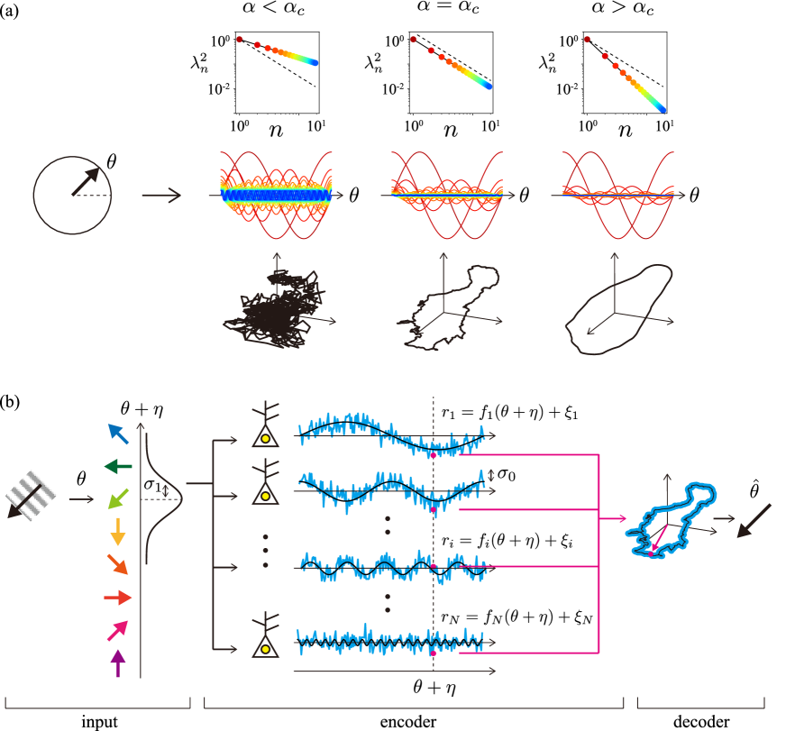
The authors of the above paper also proved that the exponent is the critical value as the exponent gives the border of differentiability of the coding manifold, and therefore the brain is in the so-called “edge of chaos”. They proved mathematically that, in the limit of large number of neurons, if the map defined by the coding from the input space to the space of the neural activity is differentiable, i.e., its neural manifold is differentiable, the eigenspectrum should asymptotically decay faster than the critical exponent . Conversely, if the eigenspectrum decays slower than the exponent, the map must be non-differentiable, and the neural response will be fractal, which means that the coding must be too sensitive to input perturbations because even infinitesimally close two inputs elicit significantly different neural activities. It is then conjectured that the brain strikes a balance between the expressiveness and robustness of the coding, because the critical power-law coding is as sensitive to inputs as possible while maintaining its smoothness. The similar critical sensitivity to perturbations also plays an important role in studies of machine learning [17, 18, 19, 20, 21, 22, 23, 24].
It is truly fascinating that the brain’s signal encoding is in a critical state on the edge of chaos[25, 26, 27, 28, 29, 30, 31]. However, quantitative evaluation of the ability of the power-law coding remain elusive probably due to the lack of the framework to describe coding ability of the power-law theoretically. For example, it remains unclear how the non-differentiability of the neural manifold indeed affect the coding performance, and why the critical state is used by the brain as an encoder.
Here, we address this problem by adopting the framework of statistical parameter estimation to the power-law coding with properly accounting for possible noise sources of it [32, 33, 34, 35, 36, 37]. In this framework, a desirable neural coding is defined as the one that allow decoders to estimate its encoded signals with minimal estimation error. This ability of the stochastic coding is measured by its Fisher information because the inverse of the Fisher information of the stochastic coding gives the lower bound of the variance of the estimation error for unbiased decoders (Cramer-Rao bound) and the asymptotic variance of the error for maximum likelihood decoders in the large number limit of observations [33, 38].
We will derive analytical expressions for the Fisher information of the neural power law coding and prove that (i) the exponent does indeed give the critical point in the sense that its Fisher information is discontinuous only at this exponent in the limit of the large numbers of neurons. Unexpectedly, however, we will see that (ii) the Fisher information is kept constant rather than decreases even for the exponent smaller than the critical value and thus for the case where its coding manifold is non-differentiable. Thus, contrary to the previous conjecture, the critical power law is not always the best coding in the information-theoretic sense. So why does the brain use the critical coding? We will show that (iii) the introduction of the energetic cost ensures that the critical coding always achieves optimality. In the derivation of Fisher information, we will also prove the remarkable relationship between the variance and the susceptibility of neural activity, corresponding to the fluctuation-dissipation theorem in statistical physics [39]. To confirm the theoretical predictions and to verify the optimality of the critical coding, we directly construct a maximum likelihood decoder for the power-law coding by explicitly integrating the conditional probability distribution of the encoded input signal. This allows us to measure the variance of its estimation errors and to numerically evaluate the Fisher information of the power-law coding.
II Results
II.1 Statistical estimation with the power-law population coding
Following Stringer’s pioneering work, let us start from the simplest case where a population of neurons encodes a one-dimensional periodic scalar angular variable, , such as the orientation of a line segment presented in animal’s visual field, thus (Fig. 1b). Generalizations to higher input dimensions will be given later. This coding can be affected by two different noise sources; one is the input noise that is put directly to the input stimulus and the other is the neural noise being independently put on each neural activity evoked by the input stimulus. We model the input noise and the neural noise for the th neuron using the independent Gaussian random variables satisfying that , , and , where and are the strengths of the input and neural noise, respectively. Then, based on the experimental results that the variance of the principal components, i.e., the eigenspectrum of the covariance matrix of the neural activities, decays with the power law in ascending order of its frequency, we express the neural activity of the th neuron () as an expansion over the orthonormal Fourier basis of a scalar periodic function,
where
Here, is an orthogonal matrix that rotates the axes of the basis function to the axes of the neuron space, and is a scaling factor that determines the magnitude of the activity of the neurons. However, by using a basis change, we can set to be the identity matrix and without loss of generality, which gives the stochastic coding model as,
| (1) |
Note that the axis change does not affect the strength of the neural noise since the noise is isotropic in the neural space.
The Fisher information of the stochastic coding is defined as the variance of the score function, the derivative of the loglikelihood function with respect to the input , or equivalently, the negative mean of the second derivative of the loglikelihood function [33, 38]
| (2) |
where denotes the probability distribution of the neuronal activity responding to the input . A variable transformation from the Gaussian variables to the neural activities gives the explicit form of the distribution function as a convolutional integral of Gaussian functions,
| (3) |
where we denote and for simplicity (See Supplemental material Sec. I for details).
II.2 Fluctuation-dissipation relationship and the Fisher information of the power-law coding
To derive an analytical expression for the Fisher information, let us assume that the noise strengths and are sufficiently small so that the probability distribution can be approximated by the multivariate Gaussian distribution,
| (4) |
where and are the mean and the covariance matrix of the neural activity for given , respectively, and denotes the transpose of .
Now let us denote the derivative of the mean with respect to the input as , namely, is the susceptibility of the mean neural activity to the input signal. Then, we can derive a remarkable relationship between the covariance matrix and the susceptibility :
| (5) |
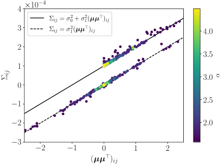
where is the identity matrix (see Supplemental material Sec. IIA for details). It should be emphasized that the relationship links the fluctuation and the susceptibility of neural activity and thus corresponds to the “fluctuation-dissipation theorem” in statistical physics, while the susceptibility appears as a second-order term rather than a linear one [39]. To confirm this significant identity we directly measure the covariance matrix and the input susceptibility for the population activity of neurons given by (1) for various realizations of the exponent , input noise , and neuron noise . Figure 2 is a scatter plot of elements of the covariance matrix versus the corresponding outer products of the susceptibility vectors . We see that regardless of the parameter realizations both diagonal (points along the solid line) and off-diagonal elements (points along the dashed line) well agrees the theoretical prediction. Thus the relationship surely satisfied for the neural coding.
The above relation also gives the impressive result that the susceptibility is an eigenvector of the covariance matrix, whose eigenvalue is given by using the generalized harmonic function , which converges to the Riemann zeta function in the limit of large numbers of neurons (see Supplemental material Sec. IIB for details),
| (6) | ||||
Putting (4) and (5) to (2) and using (6), we have the Fisher information of the power-law coding as
| (7) |
which converges to
| (8) |
in the limit of large number of neurons.
The generalization to , where neurons encodes a higher dimensional input, is almost straightforward (see Supplemental material Sec. III for details). The Fisher information for multivariate input signal is defined in the matrix form,
If the Gaussian noise with strength independently affects to the th input component , then using the same argument as above, we can show that the Fisher information matrix is diagonal and, in the limit of large numbers of neurons, the th diagonal component, which evaluates the ability of the power-law coding for the th input signal , converges to
| (9) |
where is the volume of the unit -ball. This reproduces (8) as a special case and, in the limit of large input dimension, , will converges to
| (10) |
because for large .
Figure 3 shows the derived analytical expression of the Fisher information (9) as functions of the power-law exponent for various values of the input dimension . One can see three significant features from the plots. First, the critical exponent been reported in the previous study actually gives the transition point in the sense that the derivative of the Fisher information with respect to the exponent is discontinuous only at . Second, for , each Fisher information is monotonically decreases with increasing , indicating that when the slope of the eigenspectrum of the covariance matrix is steeper than the critical slope, the coding performance deteriorates as the slope increases, which is natural because the steeper the slope the less neural activity is used in the coding.
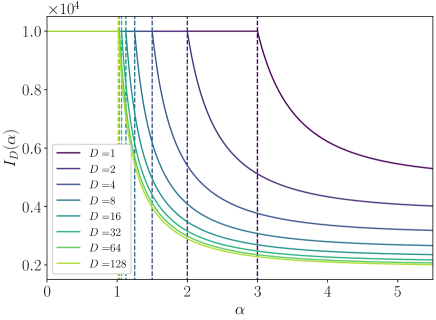
However, the third and counterintuitive point is that the Fisher information is kept constant and the coding does not degrade its performance for where the slope of the power-law decay is gentler than the critical slope, and thus, the map from the input space to the neural space defined by the coding (1) is non-differentiable and fractal even in the absence of noise. This result is different from what was previously thought. The Riemann zeta function in (9) does indeed diverge to infinity when because the zeta function diverges to infinity for . However, this does not imply either the divergence or the vanishment of the Fisher information. Rather, the information is held constant at , regardless of the neural noise strength . Thus, contrary to the previous conjecture, the coding performance is not directly related to the differentiability of the map defined by the coding.
Why does the coding not degrade its performance even in the chaotic regime where the code is extremely sensitive to the perturbation? As shown in the previous work, the map of the coding is indeed non-differentiable for . However, this non-differentiability, induced by the decrease of the power-law slope, is due to the increase of the variance of the eigenspectrum of the components with larger , i.e. higher frequencies, and importantly, the activities of the lower frequency components relatively remain intact. Thus, by using a decoder that appropriately focuses on the directions of the low-frequency components, one can still decode enough information even from the fractal neural coding, which means that the neural activity still contains enough information of the input signals and its coding performance remains intact.
II.3 Energy-information tradeoff optimizes the cortical critical power law
A natural question then is why the brain uses the critical exponent rather than one of the other smaller values of that can also achieve the best coding performance. So far, we have not considered metabolic, or energetic, costs required for the neural activities [40, 41]. However, in fact, the smaller implies that the larger amount of neural activity is evoked to represent the input signals, which may explain the optimality of the exponent for the brain’s encoding.
To see that this is indeed the case, we introduce a performance measure of the signal encoding with including an energetic cost of neural activity. Whereas the biologically realistic description of the metabolic cost of neural activity is beyond the scope of the present work, a natural definition of this will be the sum of the mean square of the response activities of all neurons over the input stimuli and the noise, which converges to the zeta function in the limit of large numbers of neurons in the present setting:
Therefore, the sum of the Fisher information and the energy cost gives an energy-aware performance measure of the power-law coding
| (11) |
where the regularization parameter must satisfy because lower energy consumption is desirable.
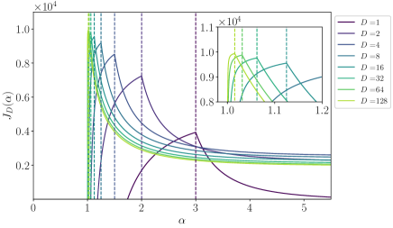
Figure 4 shows the energy-aware performance Eq. (11) as functions of the exponent for various values of the input dimension . In contrast to Fig. 3, the performances are maximized at the critical exponent , regardless of the input dimension. This result is natural because the first term of the energy-aware performance is flat for as shown in Fig. 3, while the second term of the energy cost given by the negative zeta function is a monotonically increasing with . In other words, while we have used arbitrarily small values of for the plot, the result is robust to the actual choice of values of the regularization coefficient unless it is too large to overwhelm the first term (see Supplemental material for details). The same argument also implies that the energy term need not be the sum of the square of the neural activity in order to give the same optimality of the critical exponent, as long as the term is the monotonically increasing function of . Thus, we can conclude that, for a broad class of energy terms, the trade-off between Fisher information and energy consumption explains the optimality of the critical exponent observed in the brain.
II.4 Maximum likelihood estimator for the power-law code
To validate the theoretical predictions, we actually construct the maximum likelihood decoder for the power-law coding and directly measure the variance of the estimation errors of the input stimulus to compare it with the inverse of the predicted Fisher information. For a given set of observations of neural activities responding to the input stimulus , the log-likelihood function of the input stimulus is given by
| (12) |
where, is the probability density function given by (3). We prepare a set of realizations of the activity of neurons based on (1), then put them into the log-likelihood function (12) and numerically integrate probability distributions (3) for values of to find the maximum likelihood estimate for the neural activity, i.e., the value of that maximizes the log-likelihood function (Fig. 5). By repeating the procedure, we compute the inverse of the variance of the estimates, which must asymptotically converge to the Fisher information in the limit of large numbers of observations due to the Cramer-Rao theorem.
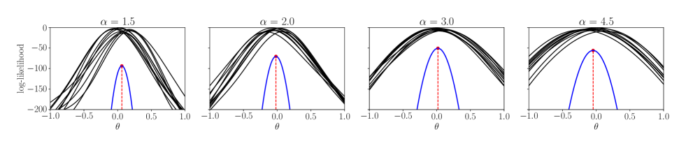
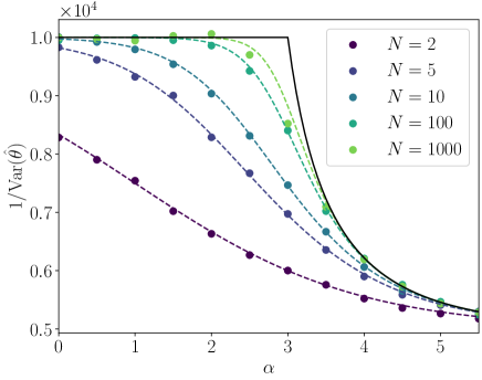
Figure 6 shows the numerically obtained inverse of the variance of the estimation error as functions of the power-law exponent for various values of . Each dotted line corresponds to the derived Fisher information, Eq. (7). One can confirm that numerical results well agree with the analytical predictions, and they monotonically converge to the solid line representing the Fisher information in the limit of large number of neurons, Eq. (8).
III Discussion
To provide a quantitative evaluation of the coding ability of the power-law stimulus representation of the population of cortical neurons, we have developed an analytically tractable model of neural coding whose spectrum of the covariance matrix follows the power law observed experimentally in the cortex. Owing to the remarkable relationship connecting the variance and the susceptibility of neural responses to the input stimuli, that is, a kind of fluctuation-dissipation theorem of neural responses, the theory allows us to explicitly derive the Fisher information of the power-law coding. Contrary to previous conjectures, the derived Fisher information demonstrates that neural coding ability is not degraded even in non-differentiable and fractal neural manifolds, where neural responses must be largely perturbed by noise included in input signals and neural activities. Conversely, our findings indicate that the introduction of a minimal metabolic cost of neural activities robustly makes the critical power-law neural response the optimal neural coding. Therefore, the experimentally observed power-law exponent gives the best balance between the energetic cost and the Fisher information of the neural coding. Consequently, the critical response observed in the brain does not merely achieve a balance between the expressivity and the robustness of the coding; it additionally strikes a balance between these two factors and the energetic cost, which must be a crucial factor for biological computation in the real world.
In this paper, assuming the visual cortex that the power-law response has been experimentally confirmed, we have restricted ourselves to the case where the input stimuli to the neurons are expressed by Fourier basis functions. However, as shown by the fluctuation-dissipation relationship, the basic framework developed cannot be restricted to the Fourier basis receptive field, whereas the actual expression of the Fisher information and the details of the tradeoff between energetic and information costs may differ from the result of the paper. For instance, introducing the Gabor filter-type receptive field, which is closer to the actual realization of the biological realization than the simple Fourier receptive field discussed here, may give an additional factor in the representation of the Fisher information. Moreover, since stimulus responses and receptive fields are generally different across cortical areas responsible for different modalities, these varieties may make different power-law exponents the critical one that realizes the best balance of energy-info tradeoff. Because recent experiments started to report that the experimentally observed power-law exponent slightly differs across areas of the cortex and across species [42, 31], it would be an important future task to apply the theory to stimulus representation with various receptive fields used in cortical regions for other modalities to reveal relationships between the observed exponents and characteristic features, such as data structure of input stimuli, across modalities.
We have introduced the power-law dependency of neural activities, a priori, here and assumed that each neuron independently responds to its stimulus with the power-law amplitude. However, it is naturally expected that this power-law dependency itself must be realized in a network of neurons that is activated by external or internal signals with some correlation. Pioneering studies have revealed that the Fisher information is generally influenced by the activity correlation [35, 37] whereas its effect is not very large when the correlation is originated from recurrent neural activities [37]. Correlation of neurons can also be very important here because it must directly be related to the power-law responses because the power-law appears in eigenspectral of the covariance matrix of response neural activities. While it remains a possibility that the covariance is purely induced by the structure of the input connections to the encoder neurons, it seems more natural that the covariance, and thus the power-law itself, is originated form interaction of the input and recurrent connections among encoder neurons [43, 44, 45]. Developing analysis of the power-law coding with combining theories of neural correlation of recurrent networks is thus important. Temporal structure of neural responses such as transient neural activities, for instance, may play an important role in these cases [46, 47]. It is also interesting remaining work to confirm the theoretical predictions by using network of realistic neuron models.
The theory developed here bears a striking resemblance to a framework of the Shannon-Hartley theorem of information theory describing the capacity of an analog communication channel under the limitation of signal power [38]. The theory states that the channel capacity, i.e., the upper bound of the information rate of the data can be transmitted through the channel without error, is given as the function of the ratio of the strengths of input signals and the additive white Gaussian noise. One can easily see the similarity between the communication using the noisy channel and the flow of the stimulus representation, that is, from the encoding of input stimulus to the activity of the population of neurons to the decoding of the value from the neural activity (Fig. 1a). Studies to find closer relationships between them must be an interesting future direction.
Because the Principal Component Analysis is based on a covariance matrix of neural activities, it can give only a linear structure of the neural manifold, whereas the manifold can generally have a higher-order structure [48]. Thus, geometric indices such as curvature of the neural manifold may play an important role in the optimal stimulus encoding in addition to the power-law exponent of the eigenspectral of the covariance matrix. Because the Fisher information matrix works as a suitable metric of statistical manifolds of probability distributions, it will also be an interesting future direction to extend the theory of optimal coding on the neural manifolds to include higher-order structures considering the information geometry [49].
Another important critical phenomenon observed for populations of cortical neurons is neural avalanche, in which the size and the duration of spontaneously generated neural activity follow the power-law distribution [25, 26, 29]. Along with the power-law coding discussed in this study, the power-law distribution of the neural avalanche also gives strong evidence that actual cortical networks work in the so-called edge-of-chaos region, which is near the critical transition point of the stability of neural responses. While the relationship between the criticality of the neural avalanche and that of the power-law coding has not been clarified yet, probably because the former considers only spontaneous activities while the latter does only stimulus-evoked activities, we can naturally expect that these two critical phenomena have a tight relationship because both of them essentially refer critical correlation structure of neural activities. As mentioned in the above section, extending the theory developed here to recurrent networks of neurons might help to reveal the hidden relation between these two neural criticalities.
Acknowledgements
T. T. discloses support for the research of this work by JST SPRING Grant Number JPMJSP2110. J. T. discloses support for publication of this work by JSPS KAKENHI Grant Number 24K15104 and 23K21352, and Japan Agency for Medical Research and Development (AMED) AMED-CREST 23gm1510005h0003.
References
- Barlow et al. [1961] H. B. Barlow et al., Possible principles underlying the transformation of sensory messages, Sensory communication 1, 217 (1961).
- Simoncelli and Olshausen [2001] E. P. Simoncelli and B. A. Olshausen, Natural image statistics and neural representation, Annu. Rev. Neurosci. 24, 1193 (2001).
- Churchland et al. [2012] M. M. Churchland, J. P. Cunningham, M. T. Kaufman, J. D. Foster, P. Nuyujukian, S. I. Ryu, and K. V. Shenoy, Neural population dynamics during reaching, Nature 487, 51 (2012).
- Rigotti et al. [2013] M. Rigotti, O. Barak, M. R. Warden, X.-J. Wang, N. D. Daw, E. K. Miller, and S. Fusi, The importance of mixed selectivity in complex cognitive tasks, Nature 497, 585 (2013).
- Sadtler et al. [2014] P. T. Sadtler, K. M. Quick, M. D. Golub, S. M. Chase, S. I. Ryu, E. C. Tyler-Kabara, B. M. Yu, and A. P. Batista, Neural constraints on learning, Nature 512, 423 (2014).
- Chung et al. [2018] S. Chung, D. D. Lee, and H. Sompolinsky, Classification and geometry of general perceptual manifolds, Phys. Rev. X 8, 031003 (2018).
- Gallego et al. [2018] J. A. Gallego, M. G. Perich, S. N. Naufel, C. Ethier, S. A. Solla, and L. E. Miller, Cortical population activity within a preserved neural manifold underlies multiple motor behaviors, Nat. Commun. 9, 4233 (2018).
- Stringer et al. [2019] C. Stringer, M. Pachitariu, N. Steinmetz, M. Carandini, and K. D. Harris, High-dimensional geometry of population responses in visual cortex, Nature 571, 361 (2019).
- Gallego et al. [2020] J. A. Gallego, M. G. Perich, R. H. Chowdhury, S. A. Solla, and L. E. Miller, Long-term stability of cortical population dynamics underlying consistent behavior, Nat. Neurosci. 23, 260 (2020).
- Yoshida and Ohki [2020] T. Yoshida and K. Ohki, Natural images are reliably represented by sparse and variable populations of neurons in visual cortex, Nat. Commun. 11, 872 (2020).
- Chung and Abbott [2021] S. Chung and L. F. Abbott, Neural population geometry: An approach for understanding biological and artificial neural networks, Curr. Opin. Neurobiol. 70, 137 (2021).
- Sorscher et al. [2022] B. Sorscher, S. Ganguli, and H. Sompolinsky, Neural representational geometry underlies few-shot concept learning, Proc. Natl Acad. Sci. USA 119, e2200800119 (2022).
- Rust and Cohen [2022] N. C. Rust and M. R. Cohen, Priority coding in the visual system, Nat. Rev. Neurosci. 23, 376 (2022).
- Nogueira et al. [2023] R. Nogueira, C. C. Rodgers, R. M. Bruno, and S. Fusi, The geometry of cortical representations of touch in rodents, Nat. Neurosci. 26, 239 (2023).
- Schneider et al. [2023] S. Schneider, J. H. Lee, and M. W. Mathis, Learnable latent embeddings for joint behavioural and neural analysis, Nature 617, 360 (2023).
- Manley et al. [2024] J. Manley, S. Lu, K. Barber, J. Demas, H. Kim, D. Meyer, F. M. Traub, and A. Vaziri, Simultaneous, cortex-wide dynamics of up to 1 million neurons reveal unbounded scaling of dimensionality with neuron number, Neuron 112, 1694 (2024).
- Poole et al. [2016] B. Poole, S. Lahiri, M. Raghu, J. N. Sohl-Dickstein, and S. Ganguli, Exponential expressivity in deep neural networks through transient chaos, Adv. Neural Inf. Proc. Sys. 29, 3368 (2016).
- Schoenholz et al. [2017] S. S. Schoenholz, J. Gilmer, S. Ganguli, and J. Sohl-Dickstein, Deep information propagation, in International Conference on Learning Representations, edited by ”” (2017).
- Pennington et al. [2017] J. Pennington, S. Schoenholz, and S. Ganguli, Resurrecting the sigmoid in deep learning through dynamical isometry: theory and practice, Adv. Neural Inf. Proc. Sys. 30, 4788 (2017).
- Kaplan et al. [2020] J. Kaplan, S. McCandlish, T. Henighan, T. B. Brown, B. Chess, R. Child, S. Gray, A. Radford, J. Wu, and D. Amodei, Scaling laws for neural language models, Preprint at https://arxiv.org/abs/2001.08361 (2020).
- Nassar et al. [2020] J. Nassar, P. A. Sokól, S. Chung, K. Harris, and I. M. Park, On 1/n neural representation and robustness, Adv. Neural Inf. Proc. Sys. 33, 6211 (2020).
- Chen et al. [2022] G. Chen, F. Scherr, and W. Maass, A data-based large-scale model for primary visual cortex enables brain-like robust and versatile visual processing, Sci. Adv. 8, eabq7592 (2022).
- Johnston and Fusi [2023] W. J. Johnston and S. Fusi, Abstract representations emerge naturally in neural networks trained to perform multiple tasks, Nat. Commun. 14, 1040 (2023).
- Joseph et al. [2023] S. Joseph, K. K. Agrawal, G. A., and B. A. Richards, On the information geometry of vision transformers, in NeurIPS 2023 Workshop on Symmetry and Geometry in Neural Representations, edited by ”” (2023).
- Beggs and Plenz [2003] J. M. Beggs and D. Plenz, Neuronal avalanches in neocortical circuits, J. Neurosci. 23, 11167 (2003).
- de Arcangelis et al. [2006] L. de Arcangelis, C. Perrone-Capano, and H. J. Herrmann, Self-organized criticality model for brain plasticity, Phys. Rev. Lett. 96, 028107 (2006).
- Tkačik et al. [2015] G. Tkačik, T. Mora, O. Marre, D. Amodei, S. E. Palmer, M. J. Berry, 2nd, and W. Bialek, Thermodynamics and signatures of criticality in a network of neurons, Proc. Natl Acad. Sci. USA 112, 11508 (2015).
- Dahmen et al. [2019] D. Dahmen, S. Grün, M. Diesmann, and M. Helias, Second type of criticality in the brain uncovers rich multiple-neuron dynamics, Proc. Natl Acad. Sci. USA 116, 13051 (2019).
- Fosque et al. [2021] L. J. Fosque, R. V. Williams-García, J. M. Beggs, and G. Ortiz, Evidence for quasicritical brain dynamics, Phys. Rev. Lett. 126, 098101 (2021).
- O’Byrne and Jerbi [2022] J. O’Byrne and K. Jerbi, How critical is brain criticality?, Trends Neurosci. 45, 820 (2022).
- Morales et al. [2023] G. B. Morales, S. di Santo, and M. A. Muñoz, Quasiuniversal scaling in mouse-brain neuronal activity stems from edge-of-instability critical dynamics, Proc. Natl Acad. Sci. USA 120, e2208998120 (2023).
- Seung and Sompolinsky [1993] H. S. Seung and H. Sompolinsky, Simple models for reading neuronal population codes, Proc. Natl Acad. Sci. USA 90, 10749 (1993).
- Brunel and Nadal [1998] N. Brunel and J. P. Nadal, Mutual information, fisher information, and population coding, Neural Comput. 10, 1731 (1998).
- Deneve et al. [1999] S. Deneve, P. E. Latham, and A. Pouget, Reading population codes: a neural implementation of ideal observers, Nat. Neurosci. 2, 740 (1999).
- Sompolinsky et al. [2001] H. Sompolinsky, H. Yoon, K. Kang, and M. Shamir, Population coding in neuronal systems with correlated noise, Phys. Rev. E Stat. Nonlin. Soft Matter Phys. 64, 051904 (2001).
- Quian Quiroga and Panzeri [2009] R. Quian Quiroga and S. Panzeri, Extracting information from neuronal populations: information theory and decoding approaches, Nat. Rev. Neurosci. 10, 173 (2009).
- Moreno-Bote et al. [2014] R. Moreno-Bote, J. Beck, I. Kanitscheider, X. Pitkow, P. Latham, and A. Pouget, Information-limiting correlations, Nat. Neurosci. 17, 1410 (2014).
- Cover [1999] T. M. Cover, Elements of information theory (John Wiley & Sons, 1999).
- Kubo [1966] R. Kubo, The fluctuation-dissipation theorem, Rep. Prog. Phys. 29, 255 (1966).
- Laughlin et al. [1998] S. B. Laughlin, R. R. de Ruyter van Steveninck, and J. C. Anderson, The metabolic cost of neural information, Nat. Neurosci. 1, 36 (1998).
- Lennie [2003] P. Lennie, The cost of cortical computation, Curr. Biol. 13, 493 (2003).
- Kong et al. [2022] N. C. L. Kong, E. Margalit, J. L. Gardner, and A. M. Norcia, Increasing neural network robustness improves match to macaque V1 eigenspectrum, spatial frequency preference and predictivity, PLoS Comput. Biol. 18, e1009739 (2022).
- Hu and Sompolinsky [2022] Y. Hu and H. Sompolinsky, The spectrum of covariance matrices of randomly connected recurrent neuronal networks with linear dynamics, PLoS Comput. Biol. 18, e1010327 (2022).
- Huang et al. [2022] C. Huang, A. Pouget, and B. Doiron, Internally generated population activity in cortical networks hinders information transmission, Sci. Adv. 8, eabg5244 (2022).
- Wardak and Gong [2022] A. Wardak and P. Gong, Extended anderson criticality in heavy-tailed neural networks, Phys. Rev. Lett. 129, 048103 (2022).
- Vyas et al. [2020] S. Vyas, M. D. Golub, D. Sussillo, and K. V. Shenoy, Computation through neural population dynamics, Annu. Rev. Neurosci. 43, 249 (2020).
- Dubreuil et al. [2022] A. Dubreuil, A. Valente, M. Beiran, F. Mastrogiuseppe, and S. Ostojic, The role of population structure in computations through neural dynamics, Nat. Neurosci. 25, 783 (2022).
- De and Chaudhuri [2023] A. De and R. Chaudhuri, Common population codes produce extremely nonlinear neural manifolds, Proc. Natl Acad. Sci. USA 120, e2305853120 (2023).
- Amari and Nagaoka [2000] S.-i. Amari and H. Nagaoka, Methods of information geometry, Vol. 191 (American Mathematical Soc., 2000).