Diff-Shadow: Global-guided Diffusion Model for Shadow Removal

Abstract

We propose Diff-Shadow, a global-guided diffusion model for high-quality shadow removal. Previous transformer-based approaches can utilize global information to relate shadow and non-shadow regions but are limited in their synthesis ability and recover images with obvious boundaries. In contrast, diffusion-based methods can generate better content but ignore global information, resulting in inconsistent illumination. In this work, we combine the advantages of diffusion models and global guidance to realize shadow-free restoration. Specifically, we propose a parallel UNets architecture: 1) the local branch performs the patch-based noise estimation in the diffusion process, and 2) the global branch recovers the low-resolution shadow-free images. A Reweight Cross Attention (RCA) module is designed to integrate global contextural information of non-shadow regions into the local branch. We further design a Global-guided Sampling Strategy (GSS) that mitigates patch boundary issues and ensures consistent illumination across shaded and unshaded regions in the recovered image. Comprehensive experiments on three publicly standard datasets ISTD, ISTD+, and SRD have demonstrated the effectiveness of Diff-Shadow. Compared to state-of-the-art methods, our method achieves a significant improvement in terms of PSNR, increasing from 32.33dB to 33.69dB on the SRD dataset. Codes will be released.

1 Introduction

Shadows are a phenomenon that exists when an optical image is captured with light blocked. The presence of shadows can complicate image processing as well as many subsequent vision tasks, e.g., object detection, tracking, and semantic segmentation [14]. The goal of shadow removal is to enhance the brightness of the image shadow regions and to achieve a consistent illumination distribution between shadow and non-shadow regions. The shadow removal task is essentially an image restoration task designed to utilize the information available in the shadow-affected image to recover the information lost due to light occlusion.

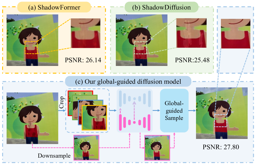
Figure 1: (a) shows the result of ShadowFormer [14], which suffers from residual shadow artifacts due to the limited modeling ability, while the result of (b) ShadowDiffusion [15] shows obvious illumination inconsistency across the images because it cannot exploit the global information. (c) exhibits the proposed Diff-Shadow, which ultimately generates high-quality shadow removal results that maintain illumination consistency and are free from block boundary artifacts through the design of a parallel network structure and a novel global-guided sampling strategy.

Shadow removal has received intensive and long-lasting studies. Traditional approaches use hand-crafted features and are based on physical lighting models [11, 47, 44]. Inspired by the successes of deep learning, many approaches that utilize large amounts of data [14, 2, 9, 49] have been introduced to improve shadow removal and reveal promising improvements. For example, Guo et al. proposed a transformer-based architecture, named ShadowFormer, to exploit non-shadow information to help shadow region restoration [14]. Their shadow-interaction module plays an important role in exploring global information. However, this kind of method often overlooks the modeling of the underlying distribution of natural images. Consequently, the generated results appear significant residual shadows, as shown in Fig. 1 (a).

Recently, diffusion models have gained wide interest in the field of image restoration [33, 34, 19] due to its powerful modeling ability. Guo et al. proposed ShadowDiffusion to jointly pursue shadow-free images and refined shadow masks [15]. Although it covers the whole input image, the simple UNet denoising architecture is not enough for exploring global information, which results in inconsistent illumination of the outputs, as shown in Fig. 1 (b). Furthermore, generating arbitrary resolution images directly with ShadowDiffusion proved challenging as diffusion models are more suitable for processing smaller patches [6]. While Zheng et al. [6] and Ozan et al. [30] proposed several patch-based diffusion methods that demonstrated exceptional performance in image restoration tasks at arbitrary resolutions, they still faced limitations when handling shadow removal task. These methods lack global contextual information and ultimately lead to lighting inconsistencies or obvious boundaries in the restored images.

Considering the powerful modeling capabilities of diffusion models and the necessity of global information for shadow removal tasks, we propose Diff-Shadow, a global-guided diffusion model for generating high-quality shadow-free results with no obvious boundaries and consistent illumination in arbitrary image resolution. Our Diff-Shadow adopts the parallel UNets network architecture that receives both patch and global inputs, where the local branch focuses on estimating patch noise, while the global branch is responsible for recovering low-resolution shadow-free images. Additionally, our Diff-Shadow exploits the global contextual information of the non-shadow region from the global branch through the Reweight Cross Attention (RCA) module. Subsequently, we present a Global-guided Sampling Strategy (GSS) within the denoising process. In this strategy, the fusion weights for patch noise are determined by considering both the brightness disparity between the recovered patch and the global image, as well as the extent of shadow regions within the patch. This approach addresses potential merging artifacts, preserves excellent illumination consistency, and ultimately enhances the overall quality of the results, as shown in Fig. 1 (c). Moreover, benefiting from the patch-based methods, the proposed Diff-Shadow can be expanded to handle images with arbitrary resolution.

To summarize, our main contributions are as follows:

• We propose Diff-Shadow, a global-guided Diffusion Model pipeline, which incorporates a parallel UNets architecture, concentrating on both the patch and global information for the effective shadow removal.

• We design a Reweight Cross Attention (RCA) module to exploit the correlation between the local branch and the non-shadow regions of the global image.

• We propose a Global-guided Sampling Strategy (GSS) to further improve the quality of shadow removal during the diffusion denoising process.

• Extensive experimental results on public ISTD [41], ISTD+ [22], and SRD [31] datasets demonstrate that the proposed Diff-Shadow outperforms the state-of-the-art shadow removal methods.

2 Related Works

Shadow Removal.

Recent learning-based methods for shadow removal tasks have achieved superior performance by leveraging large-scale high-quality training data to learn high-level image texture and semantic information [2, 9, 14, 15]. Unlike traditional physical-based methods that rely on prior assumptions like illumination [1, 47], gradient [7, 8, 27, 25, 11], and region [16, 12, 13], learning-based approaches tend to learn contextual features for shadow removal. For instance, Qu et al. proposed a multi-context embedding network to integrate multi-level information [31], while Wang et al. explored the relationship between shadow detection and removal, and proposed a stacked conditional generative adversarial network (ST-CGAN) [41]. Other works like Hu et al. [18] and Zhang et al. [48] focused on applying spatial context attention features and exploring residual-illumination relationships, respectively. These learning-based methods have produced impressive results, but there remain opportunities to further capture the correspondence between shadow and non-shadow areas.

Diffusion Methods.

Recent advances in generative diffusion models [17] , [28] and noise-conditional score networks  [36], [37] have shown powerful image synthesis capabilities [5]. By gradually corrupting images into noise and reversing the process, high-fidelity and diverse results can be sampled. Therefore, many studies have been inspired by the powerful generative capability of diffusion models and applied them to image restoration tasks, such as super-resolution [34, 10, 29, 24, 35, 32], deblurring [43, 3], denoising [45, 38], and inpainting [33, 46, 26]. These tasks have achieved promising results, with some even reaching the state-of-the-art level. For general image restoration, Özdenizci et al. proposed a patch-based denoising diffusion approach to handle arbitrary image sizes [30]. By operating on image patches, their method restored local details while maintaining global coherence via overlapping patches. As for the shadow removal task, ShadowDiffusion integrates image and degradation priors into a unified diffusion framework [15], which progressively refines the output image and the shadow mask for accurate shadow-free image generation. We design a diffusion model with parallel UNets architecture to perform the local patch noise estimation and the global image reconstruction.

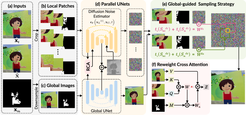
Figure 2: An overview of the proposed Diff-Shadow. The local branch of Parallel UNets performs patch diffusion noise estimation using patches of the intermediate variable $\mathbf{x}_{t}$, the shadow image $\tilde{\mathbf{x}}$, and the shadow mask $\mathbf{x}_{m}$. The latter two images are also down-sampled as inputs of the global UNet, which constructs the low-resolution shadow-free image on the one hand and provides the global contextual information of non-shaded regions $\mathbf{x}_{G}$ into the local branch ${\mathbf{x}_{L}}^{(i)}$ using the proposed Reweight Cross Attention (RCA) module on the other hand. After estimating the noises of local patches, the Global-guided Sampling Strategy (GSS) works to construct the noise distribution for the whole image. $t_{1}$ and $t_{2}$ represent functions corresponding to the step $t$.

Shadow and Non-Shadow Consistency.

Shadow removal presents a unique challenge in that shadows corrupt only parts of an image, while abundant uncorrupted information remains in non-shadowed regions. However, previous methods [22, 23] focused only on local shadow or non-shadow regions, leading to severe artifacts around shadow boundaries and inconsistent brightness between shadow and non-shadow areas. More recent approaches leverage contextual information from both shadow and non-shadow areas of the image to inform the shadow removal process. For instance, DeshadowNet [31] incorporates multi-scale information to expand the receptive field, leveraging texture and appearance information across the image. Chen et al. proposed CANet [2], using an external patch-matching module to discover texture relationships. Guo et al. introduced ShadowFormer [14], incorporating a Shadow-Interaction Module in the transformer to model the global texture. Related but divergent, we propose the Reweight Cross Attention module injected into the diffusion model, empowering it with global textural relationship modeling.

3 Method

In this section, we describe the proposed global-guided denoising diffusion model for shadow removal (Diff-Shadow). Given the intermediate variable $\mathbf{x}_{\text{t}}\in\mathbb{R}^{3\times H\times W}$, the shadow image $\tilde{\mathbf{x}}\in\mathbb{R}^{3\times H\times W}$ with corresponding shadow mask $\mathbf{x}_{m}\in\mathbb{R}^{3\times H\times W}$ in Fig. 2 (a), the proposed architecture is trained and inference using both high-resolution image patches as well as low-resolution down-sampled full images, which are optimized by the parallel UNets (Fig. 2 (d)) whose local branch performs the diffusion noise estimation of local patches and the global UNet recovers the down-sampled full shadow-free image. The global contextual information of non-shadow regions is integrated into the local branch through the RCA module (Fig. 2 (f)) and the Convolutional Aggregation (CA) during training. The Global-guided Sampling Strategy (GSS) (Fig. 2 (e)) is utilized to systematically combine the features of neighboring patches during inference. Thanks to the excellent modeling ability of the diffusion model with small-size images, the proposed Diff-Shadow achieves satisfactory performance for shadow removal tasks.

3.1 Overall Architecture

Condition diffusion model [34] have achieved impressive performance for image-conditional data synthesis and editing tasks, which learns a conditional reverse process $p_{\theta}\left(\mathbf{x}_{0:T}\mid\tilde{\mathbf{x}}\right)$ without modifying the diffusion process $q\left(\mathbf{x}_{1:T}\mid\mathbf{x}_{0}\right)$ for ${\mathbf{x}}$, such that the sampled image has high fidelity to the data distribution conditioned on $\tilde{\mathbf{x}}$. Common diffusive models train samples $\left(\mathbf{x}_{0},\tilde{\mathbf{x}}\right)\sim q\left(\mathbf{x}_{0},\tilde{\mathbf{x}}\right)$ from a paired data distributions (e.g., a clean image $\mathbf{x}_{0}$ and a degraded image $\tilde{\mathbf{x}}$), and learn a conditional diffusion model where it provides $\tilde{\mathbf{x}}$ to the reverse process:

$$\small p_{\theta}\left(\mathbf{x}_{0:T}\mid\tilde{\mathbf{x}}\right)=p\left(\mathbf{x}_{T}\right)\prod_{t=1}^{T}p_{\theta}\left(\mathbf{x}_{t-1}\mid\mathbf{x}_{t},\tilde{\mathbf{x}}\right).$$ (1)

As for shadow removal tasks with shadow masks $\mathbf{x}_{m}$, we design the parallel UNets architecture. The local branch performs the diffusion noise estimation and is conditioned by image patches: ${\mathbf{x}_{L}}^{(i)}=\left\{\tilde{{\mathbf{x}}}^{(i)},{\mathbf{x}_{m}}^{(i)}\right\}$, where $\tilde{\mathbf{x}}^{(i)}=\operatorname{Crop}\left(\boldsymbol{L}_{i}\circ\tilde{\mathbf{x}}\right)$ and ${\mathbf{x}_{m}}^{(i)}=\text{Crop}\left(\boldsymbol{L}_{i}\circ\mathbf{x}_{m}\right)$ represent $R\times R$ patches, and $\text{Crop}(\cdot)$ extracts the patches from the location $\boldsymbol{L}_{i}$. The estimated noise of local patches will be combined during the inference through the proposed GSS modules (Fig. 2 (e)), which is described in Sec. 3.3. The global branch is optimized by the low-resolution down-sampled full images: $\mathbf{x}_{G}=\left\{\tilde{{\mathbf{x}}}^{\prime},{\mathbf{x}_{m}}^{\prime}\right\}$. The contextual information of non-shadow regions plays an auxiliary role and is integrated into the local branch through the RCA module (Fig. 2 (f)), which is described in Sec. 3.2. Therefore, the reverse process in Eq. 1 can be expanded as:

$$\footnotesize p_{\theta}\!\left(\mathbf{x}_{0:T}^{(i)}\!\mid\!{\mathbf{x}_{L}}^{(i)},\mathbf{x}_{G}\right)\!=\!p\left(\mathbf{x}_{T}^{(i)}\right)\prod_{t=1}^{T}p_{\theta}\!\left(\mathbf{x}_{t-1}^{(i)}\!\mid\!\mathbf{x}_{t}^{(i)},{\mathbf{x}_{L}}^{(i)},\mathbf{x}_{G}\right),$$ (2)

where ${\mathbf{x}_{0}}^{(i)}=\text{Crop}\left(\boldsymbol{L}_{i}\circ\mathbf{x}_{0}\right)$. The training approach is outlined in Algorithm 1.

We can sample the intermediate $\mathbf{x}_{t}$ from the clean image $\mathbf{x}_{0}$ through $\mathbf{x}_{t}=\sqrt{\bar{\alpha}_{t}}\mathbf{x}_{0}+\sqrt{1-\bar{\alpha}_{t}}\boldsymbol{\epsilon}$, where $\alpha_{t}=1-\beta_{t}$, $\beta_{t}$ is a predefined variance schedule, $\bar{\alpha}_{t}=\prod_{i=1}^{t}\alpha_{i}$, and $\boldsymbol{\epsilon}\sim\mathcal{N}(\mathbf{0},\mathbf{I})$. The model is trained to predict the noise by:

$$\small\boldsymbol{{\epsilon}_{t}}=\boldsymbol{\epsilon}_{\theta}\left(\sqrt{\bar{\alpha}_{t}}{\mathbf{x}_{0}}^{(i)}+\sqrt{1-\bar{\alpha}_{t}}\boldsymbol{\epsilon},{\mathbf{x}_{L}}^{(i)},\mathbf{x}_{G},t\right).$$ (3)

Algorithm 1 Diffusive shadow removal model training

0:  shadow image $\tilde{\mathbf{x}}$, clean image $\mathbf{x}_{0}$ and mask $\mathbf{x}_{m}$

1:  repeat

2:     Randomly sample a patch $\boldsymbol{L}_{i}$

3:      $\mathbf{x}_{0}^{(i)}=\operatorname{Crop}\left(\boldsymbol{L}_{i}\circ\mathbf{x}_{0}\right)$

4:     $\mathbf{x}_{L}{}^{(i)}=\left\{\tilde{\mathbf{x}}^{(i)},\mathbf{x}_{m}{}^{(i)}\right\}$ where $\tilde{\mathbf{x}}^{(i)}=\operatorname{Crop}\left(\boldsymbol{L}_{i}\circ\tilde{\mathbf{x}}\right)$ and $\mathbf{x}_{m}^{(i)}=\operatorname{Crop}\left(\boldsymbol{L}_{i}\circ\mathbf{x}_{m}\right)$

5:     $\mathbf{x}_{G}=\left\{\tilde{\mathbf{x}}^{\prime},{\mathbf{x}_{m}}^{\prime}\right\}$ where $\tilde{\mathbf{x}}^{\prime}=\operatorname{Dowmsample}(\tilde{\mathbf{x}})$ and ${\mathbf{x}_{m}}^{\prime}=\operatorname{Dowmsample}(\mathbf{x}_{m})$

6:     $t\sim\text{Uniform}\{1,\ldots,T\}$

7:     $\boldsymbol{\epsilon}\sim\mathcal{N}(\mathbf{0},\mathbf{I})$

8:     Perform a gradient descent step for   $\nabla_{\theta}\left\|\boldsymbol{\epsilon}_{t}-\boldsymbol{\epsilon}_{\theta}\left(\sqrt{\bar{\alpha}_{t}}\mathbf{x}_{0}^{(i)}+\sqrt{1-\bar{\alpha}_{t}}\boldsymbol{\epsilon},{\mathbf{x}_{L}}^{(i)},\mathbf{x}_{G},t\right)\right\|^{2}$

9:  until converged

10:  return  $\theta$

3.2 Reweight Cross Attention

Existing patch-based approaches lack generality since the regions inside a patch may all be corrupted for shadow removal tasks. Apart from the local patch-based diffusion branch, we introduce a parallel global UNet to recover low-resolution shadow-free images. The Reweight Cross Attention (RCA) module is introduced to integrate the global information into the local patch by combining the low-level features. As shown in Fig. 2 (f), the output of RCA can be summarized as:

$$Z=\operatorname{softmax}\left(\frac{\mathbf{Q}\mathbf{K}^{T}}{d}\right)\mathbf{M}\mathbf{V},$$ (4)

where $\mathbf{Q}$ represents the projected queries of patch features, $\mathbf{K}$ and $\mathbf{V}$ are the projected keys and values of global image features, $d$ is the scaling parameter, and $\mathbf{M}$ is the binary mask to multiply with the features. Attention maps between $\mathbf{Q}$ and $\mathbf{K}$ are first calculated to capture mutual information between pixels in the local branch and regions in the global branch. Subsequently, the mask is introduced to assist in suppressing mutual information values in the global shadow regions. The adjusted attention map is then multiplied by the global $\mathbf{V}$ vector to obtain the expected global information for the local branch.

We interact the low-level features of the first convolutional block in the global UNet with the corresponding layer in the local UNet through the RCA module because low-level features concentrate more on image edges, colors, and corners, which are important for shadow removal tasks. As for high-level abstract features, we apply a simple concatenation to achieve interaction. In contrast to recent cross-attention modules in Shadowformer [14] whose $\mathbf{Q}$, $\mathbf{K}$ and $\mathbf{V}$ originate from the same global feature, the RCA integrates both local and global information. Furthermore, other attention-based methods boost the mutual information between shadow and non-shadow pairs through masks. However, the shadow information is dispensable for recovering non-shadow regions. Contrarily, our attention mechanism utilizes masks to suppress the global shadow values through the attention map, integrating the more important non-shadow information from the global branch into the local branch.

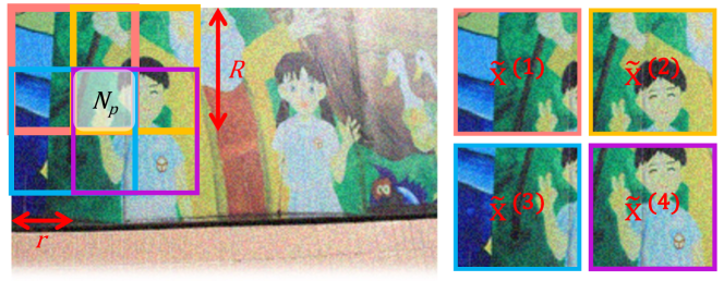
Figure 3: The illustration of noise merge for overlapping patches. $N_{p}$ represents the number of overlapping patches for each pixel. $r$ and $R$ are the step size and the patch size.

3.3 Global-guided Samping Strategy

To overcome the shortcomings of merging artifacts from independently intermediate patches, Ozdenizci et al. proposed to perform reverse sampling based on the mean estimated noise for each pixel in overlapping patch regions, which works better for weather image with relatively unified degradation [30]. However, as for shadow removal tasks with extreme inconsistencies between shadow and non-shadow regions, predicting mean estimated noise lacks ability to achieve a consistent illumination distribution. Therefore, we propose the Global-guided Sampling Strategy (GSS) to preserve excellent illumination consistency.

The general idea of patch-based restoration is to operate locally on patches extracted from the image and optimally merge the results.

We consider a grid-like arranged parsing scheme over the intermediate variable $\mathbf{x}_{t}$, the shadow image $\tilde{\mathbf{x}}$ and the shadow mask $\mathbf{x}_{m}$, and extract all patches by moving over the $R\times R$ grid with a step size of $r$ in both horizontal and vertical dimensions, as shown in Fig. 3. During patch-based diffusive image restoration, we perform noise estimation based on adaptive estimated noise for each pixel in overlapping patch regions, at any given denoising time step $t$. As shown in Fig. 2 (e), the weight of each patch is determined by two parts: the brightness-based score $S_{\text{bri}}$ and the mask-based score $S_{\text{m}}$. The former one considers the brightness consistency of the local patches and the global images, while the latter one corresponds to the proportion of shadow and non-shadow regions.

The brightness-based score $S_{\text{bri}}$ constrains that the patch recovered by the local branch should show similar brightness with the full image generated by the global branch. The $S_{\text{bri}}$ is defined as:

$$\small S_{\text{bri}}=1-\frac{\mathrm{avg}{(|L_{\text{gray}}-G_{\text{gray}}|)}}{\mathrm{max}({(|L_{\text{gray}}-G_{\text{gray}}|)})+\mathrm{eps}},$$ (5)

where $L_{\text{gray}}$ is the recovered gray image of the local patch, $G_{\text{gray}}$ is the recovered gray image of global image.

In addition, the masked-based score $S_{\text{m}}$ pays more attention to non-shadow regions. When the non-shadow region dominates the image patch, the receptive field of the local branch encompasses both shadow and non-shadow regions, providing a valuable way to eliminate shadows through non-shadow information. Conversely, when the non-shadow region dominates the image patch, the predicted illumination may mainly originate from the global branch, whose performance tends to be unsatisfactory. Based on the binary mask, the ratio of non-shadow region among the patch can be calculated through: $R_{\text{sf}}=P_{\text{sf}}/P_{\text{total}}$, where $P_{\text{sf}}$ is the number of non-shadow pixels and $P_{\text{total}}$ is the number of total patch pixels. The mask-based score $S_{\text{m}}$ is defined as:

$$\small S_{\text{m}}=\left\{\begin{array}[]{cc}1&R_{\text{sf}}\geq T_{\text{sf}}\\ R_{\text{sf}}/{T_{\text{sf}}}&R_{\text{sf}}<T_{\text{sf}}\end{array},\right.$$ (6)

where $T_{\text{sf}}$ is the threshold of the ratio. In our implementation, $T_{\text{sf}}$ is set to 0.5 and $\mathrm{eps}$ is set to 0.01.

The weights of each patch contributed to constructing the full noise map are calculated as:

$$\small W^{d}=\frac{t\cdot S_{\text{bri}}}{T}+\frac{(T-t)\cdot S_{\text{m}}}{T},$$ (7)

where $T$ is the total steps. The final adaptive estimated noise is computed as:

$$\small\frac{1}{\sum_{i}W^{d_{i}}}\sum_{i=1}^{N_{p}}\left(W^{d_{i}}\!\cdot\!\epsilon_{\theta}\left(\mathbf{x}_{t}^{(i)},{\mathbf{x}_{L}}^{(i)},{\mathbf{x}_{G}},t\right)\right),$$ (8)

where $i\in\left\{1,\ldots,N_{p}\right\}$ and $N_{p}$ is the number of overlapping patches of each pixel. The test time diffusive image restoration method is outlined in Algorithm 2.

Algorithm 2 Global-guided diffusive image restoration

0:  shadow image $\tilde{\mathbf{x}}$, shadow mask $\mathbf{x}_{m}$, conditional diffusion model $\boldsymbol{\epsilon}_{\theta}$, number of implicit sampling steps $S$, dictionary of $D$ overlapping patch locations.

1:  $\mathbf{x}_{t}\sim\mathcal{N}(\mathbf{0},\mathbf{I})$

2:  for $i=S,\ldots,1$ do

3:     $t=(i-1)\cdot T/S+1$

4:     $t_{\text{next }}=(i-2)\cdot T/S+1$ if $i>1$ else 0

5:     $\hat{\boldsymbol{\Omega}}_{t}=0$ and $M=0$

6:     for $d=1,\ldots,D$ do

7:        $\mathbf{x}_{t}^{(d)}=\operatorname{Crop}\left(\boldsymbol{L}_{d}\circ\mathbf{x}_{t}\right)$

8:        $\mathbf{x}_{L}{}^{(d)}\!=\!\left\{\tilde{\mathbf{x}}^{(d)},\mathbf{x}_{m}{}^{(d)}\right\}$ where $\tilde{\mathbf{x}}^{(d)}\!=\!\operatorname{Crop}\left(\boldsymbol{L}_{d}\circ\tilde{\mathbf{x}}\right)$ and ${\mathbf{x}_{m}}^{(d)}\!=\!\operatorname{Crop}\left(\boldsymbol{L}_{d}\circ\mathbf{x}_{m}\right)$

9:        $\mathbf{x}_{G}=\left\{\tilde{\mathbf{x}}^{\prime},{\mathbf{x}_{m}}^{\prime}\right\}$ where $\mathbf{x}^{\prime}=\operatorname{Dowmsample}(\mathbf{x})$ and ${\mathbf{x}_{m}}^{\prime}=\operatorname{Dowmsample}(\mathbf{x}_{m})$

10:        $\hat{\boldsymbol{\Omega}}_{t}=\hat{\boldsymbol{\Omega}}_{t}+W^{d}\cdot\boldsymbol{\epsilon}_{\theta}\left(\mathbf{x}_{t}^{(d)},\tilde{\mathbf{x}_{L}}^{(d)},\mathbf{x}_{G},t\right)$

11:        $M=M+W^{d}$

12:     end for

13:     $\hat{\boldsymbol{\Omega}}_{t}=\hat{\boldsymbol{\Omega}}_{t}/M$

14:     $\mathbf{x}_{t}\leftarrow\sqrt{\bar{\alpha}_{t_{\text{next }}}}\left(\frac{\mathbf{X}_{t}-\sqrt{1-\bar{\alpha}_{t}}\cdot\hat{\boldsymbol{\Omega}}_{t}}{\sqrt{\bar{\alpha}_{t}}}\right)+\sqrt{1-\bar{\alpha}_{t_{\text{next }}}}\cdot\hat{\boldsymbol{\Omega}}_{t}$

15:  end for

16:  return  $\mathbf{x}_{t}$

3.4 Optimization

The Diff-Shadow involves two parallel UNet networks operating the local patch optimization and the global shadow-free image reconstruction. The objective function includes the following two items: the diffusive objective function $L_{\text{diff}}$ and the global loss function $L_{\text{global}}$.

$$\small\mathcal{L}_{\text{total }}=\mathcal{L}_{\text{diff }}+\lambda\mathcal{L}_{\text{global}},$$ (9)

where $\lambda$ is a hyper-parameter to balance the contributions of the two losses. We empirically set it to 1.

The Diffusive Objective Function. Refer to [17], the $\mathcal{L}_{\text{diff}}$ is defined as:

$$\small\mathcal{L}_{\text{diff}}=\mathbb{E}_{\mathbf{x}_{0},t,\boldsymbol{\epsilon}}\left\|\boldsymbol{{\epsilon}}_{t}-\boldsymbol{\epsilon}\right\|_{F}^{2}.$$ (10)

The Global Loss Function. The global UNet recovers shadow-free images from down-sampled shadow images and mask images:

$$\small\mathcal{L}_{\text{global}}=\mathbb{E}_{\mathbf{{x}_{0}}^{\prime},\mathbf{{x}_{m}}^{\prime}}\left\|\mathbf{x}_{r}-\mathbf{{x}_{0}}^{\prime}\right\|_{F}^{2},$$ (11)

where $\mathbf{x}_{r}$ is the global output, $\mathbf{{x}_{0}}^{\prime}$ and $\mathbf{{x}_{m}}^{\prime}$ are the down-sampled clean images and shadow mask, respectively.

4 Experiments

Dataset	Method	Shadow Regions (S)			Non-Shadow Regions (NS)			All Image (All)
		PSNR$\uparrow$	SSIM$\uparrow$	RMSE$\downarrow$	PSNR$\uparrow$	SSIM$\uparrow$	RMSE$\downarrow$	PSNR$\uparrow$	SSIM$\uparrow$	RMSE$\downarrow$
ISTD [41]	Input Image	22.40	0.936	32.10	27.32	0.976	7.09	20.56	0.893	10.88
	Guo et al. [16]	27.76	0.964	18.65	26.44	0.975	7.76	23.08	0.919	9.26
	ST-CGAN [41]	33.74	0.981	9.99	29.51	0.958	6.05	27.44	0.929	6.65
	DHAN [4]	35.53	0.988	7.49	31.05	0.971	5.30	29.11	0.954	5.66
	Fu et al. [9]	34.71	0.975	7.91	28.61	0.880	5.51	27.19	0.945	5.88
	DC-ShadowNet [20]	31.69	0.976	11.43	28.99	0.958	5.81	26.38	0.922	6.57
	Zhu et al. [50]	36.95	0.987	8.29	31.54	0.978	4.55	29.85	0.960	5.09
	ShadowFormer [14]	38.19	0.991	5.96	34.32	0.981	3.72	32.21	0.968	4.09
	ShadowDiffusion [15]	40.15	0.994	4.13	33.70	0.977	4.14	32.33	0.969	4.12
	Ours	39.71	0.994	1.41	35.58	0.987	2.48	33.69	0.976	2.89
SRD [31]	Input Image	18.96	0.871	36.69	31.47	0.975	4.83	18.19	0.830	14.05
	Guo et al. [16]	-	-	29.89	-	-	6.47	-	-	12.60
	DeshadowNet [31]	-	-	11.78	-	-	4.84	-	-	6.64
	DHAN [4]	33.67	0.978	8.94	34.79	0.979	4.80	30.51	0.949	5.67
	Fu et al. [9]	32.26	0.966	9.55	31.87	0.945	5.74	28.40	0.893	6.50
	DC-ShadowNet [20]	34.00	0.975	7.70	35.53	0.981	3.65	31.53	0.955	4.65
	BMNet [49]	35.05	0.981	6.61	36.02	0.982	3.61	31.69	0.956	4.46
	SG-ShadowNet [40]	-	-	7.53	-	-	2.97	-	-	4.23
	Zhu et al. [50]	34.94	0.980	7.44	35.85	0.982	3.74	31.72	0.952	4.79
	ShadowFormer [14]	36.91	0.989	5.90	36.22	0.989	3.44	32.90	0.958	4.04
	ShadowDiffusion [15]	38.47	0.987	4.98	37.78	0.985	3.44	34.73	0.957	3.63
	Ours	37.91	0.988	1.81	39.49	0.990	1.65	34.93	0.977	2.52
ISTD+ [22]	Input Image	18.96	0.871	36.69	31.47	0.975	4.83	18.19	0.830	14.05
	ST-CGAN [41]	-	-	13.40	-	-	7.70	-	-	8.70
	DeshadowNet [31]	-	-	15.90	-	-	6.00	-	-	7.60
	Fu et al. [9]	36.04	0.976	6.60	31.16	0.876	3.83	29.45	0.840	4.20
	DC-ShadowNet [20]	32.20	0.976	10.43	33.21	0.963	3.67	28.76	0.922	4.78
	BMNet [49]	37.30	0.990	6.19	35.06	0.974	3.09	32.30	0.955	3.60
	SG-ShadowNet [40]	-	-	5.9	-	-	2.90	-	-	3.4
	ShadowFormer [14]	39.67	-	5.20	38.82	-	2.30	35.46	-	2.80
	ShadowDiffusion [15]	39.82	-	4.90	38.90	-	2.30	35.68	0.970	2.70
	Ours	40.63	0.993	1.30	39.69	0.989	1.57	36.47	0.979	2.09

Table 1: The quantitative results of shadow removal using our model and recent methods on ISTD [41], SRD [31] and ISTD+ [22] datasets. ‘-’ represents the values that were not reported in the original paper.

4.1 Experimental Setups

Datasets. We used three standard benchmark datasets for our shadow removal experiments: 1) ISTD dataset [41] includes 1,330 training and 540 testing triplets (shadow images, masks and shadow-free images); 2) Adjusted ISTD (ISTD+) dataset [22] reduces the illumination inconsistency between the shadow and shadow-free image of ISTD using linear regression; 3) SRD dataset [31] consists of 2,680 training and 408 testing pairs of shadow and shadow-free images without the ground-truth shadow masks. Referring to ShadowDiffusion [15], we applied the prediction mask provided by DHAN [4] for the training and testing.

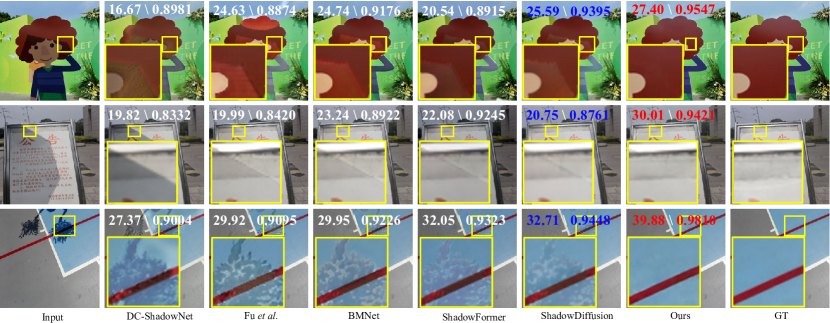
Figure 4: Qualitative comparison with DC-ShadowNet [20], Fu et al. [9], BMNet [49], ShadowFormer [14] and ShadowDiffusion [15] on ISTD+ [22]. The values represent the ‘PSNR/SSIM’. The best and second-best results are illustrated in red and blue.

Implementation Details. Our Diff-Shadow is implemented by PyTorch, which is trained using eight NVIDIA GTX 2080Ti GPUs. The Adam optimizer [21] is applied to optimize the parallel UNets with a fixed learning rate of $lr=2e^{-4}$ without weight decay and the training epoch is set as 2,000. The exponential moving average [28] with a weight of 0.999 is applied for parameter updating.

Training Specifications. For each dataset, the images are resized into $256\times 256$ for training. For each iteration, we initially sampled 8 images from the training set and randomly cropped 16 patches with size $64\times 64$ from each image plus a down-sampled global image with the same size corresponding to each patch. This process resulted in mini-batches consisting of 96 samples. We used input time step embeddings for $t$ through sinusoidal positional encoding [39] and provided these embeddings as inputs to each residual block in the local and global branches, allowing the model to share parameters across time. During sampling, the patch size $R$ is set to 64 and the step size $r$ is set to 8 for covering the whole image.

Evaluation Measures. Following previous works [16, 31, 41, 4, 9, 20, 49, 14, 15], we utilized the Root Mean Square Error (RMSE) in the LAB color space as the quantitative evaluation metric of the shadow removal results, comparing to the ground truth shadow-free images. Lower RMSE scores correspond to better performance. In addition, we also adopt the common Peak Signal-to-Noise Ratio (PSNR) and the Structural Similarity Index Measure (SSIM) [42] to measure the performance in the RGB color space.

4.2 Comparison with State-of-the-art Methods

We compare the proposed Diff-Shadow with the popular or state-of-the-art (SOTA) shadow removal algorithms, including one traditional method: Guo et al. [16], several deep learning-based methods: DeshadowNet [31], ST-CGAN [41], DHAN [4], Fu et al. [9], DC-ShadowNet [20], BMNet [49], ShadowFormer [14], and one diffusion-based method: ShadowDiffusion [15]. The shadow removal results of the competing methods are quoted from the original papers or reproduced using their official implementations. Following the previous methods [14, 15], we evaluate the shadow removal results with $256\times 256$ resolution.

Quantitative Evaluation. Table 1 shows the quantitative results on the test sets over ISTD [41], SRD [31], and ISTD+ [22], respectively. The superiority of the proposed method over competing approaches is evident across all three datasets, as it consistently achieves superior performance. Thanks to the powerful modeling capabilities of the diffusion model for images, the proposed method improves the PSNR of the SRD [31] dataset from 32.90dB (ShadowFormer) to 34.93dB (Ours) when compared with the most recent transformer-based method ShadowFormer. Furthermore, compared to ShadowDiffusion which is also a diffusion-based method, our parallel network architecture interacts the local and global information more effectively. The novel Global-guided Sampling Strategy (GSS) further enhances the accuracy of shadow-free image restoration, which results in an improvement in PSNR from 32.33dB (ShadowDiffusion) to 33.69dB (Ours) on the ISTD [41] dataset. In summary, our Diff-Shadow provides better shadow removal performance than any of the recently proposed models, achieving new state-of-the-art results on three widely-used benchmarks.

Methods	S	NS	ALL	Sampling	S	NS	ALL
(a) Single-head(w/o global)	2.64	3.41	3.36	(e) w/o GSS	2.97	3.63	3.81
(b) Single-head(w global)	2.55	3.19	3.04	(f) $W^{d}=1$	2.64	3.42	3.27
(c) Ours (w/o RCA)	2.31	2.14	2.73	(g) $S_{\text{bri}}$	2.16	2.99	2.96
(d) Ours (complete model)	1.81	1.65	2.52	(h) $S_{\text{bri}}+S_{\text{m}}$	1.81	1.65	2.52

Table 2: Ablation studies on SRD dataset [31]. We report RMSE values.

	(a)	(b)	(c)	(d)	(e)	(f)
RCA	first-layer	w/o	second-layer	first&mid-layer	w/o	first-layer
CA	w/o	mid-layer	mid-layer	w/o	every-layer	mid-layer
PSNR$\uparrow$	35.31	35.49	36.27	35.40	36.14	36.47

Table 3: Ablation studies to evaluate the effectiveness of different network structures on the ISTD+ [22] dataset.

Qualitative Evaluation. We present the qualitative comparison in Fig. 4 and the supplementary file. The proposed Diff-Shadow stands out among previous methods for its remarkable ability to remove shadows, while preserving the surrounding image textures and luminance, even in areas of high contrast that pose challenges for shadow removal. For example, in the third example of Fig. 4, there is a distinct color disparity between the ground and the shadow. Previous methods struggled to successfully remove the fragmented shadows of tree branches at this location, resulting in uneven color distribution or incomplete removal results. The result of our method is the most similar to the ground truth and surpasses the second-best approach by nearly 7dB. This further demonstrates the superiority of the proposed method in perceiving the shadow and non-shadow illumination consistency.

4.3 Ablation Studies

Effectiveness of Parallel UNets. The global branch is first removed to only accommodate the local inputs. Consequently, the network degrades to a single-head UNet structure. As in Table 2 (a), the single-head UNet shows the worst performance due to missing global context information. We tried to concatenate the patch and global images together at the network input level, and the results in Table 2 (b) show that the introduction of global context information works better than patch input alone. Then, in order to verify the effectiveness of the RCA module, we retained the two-branch network mechanism but eliminated the RCA module from the first layer and kept only the concatenate connection in the middle layer. As can be seen from Table 2 (c), the RCA module is effective in interacting two branches and enhancing the final result.

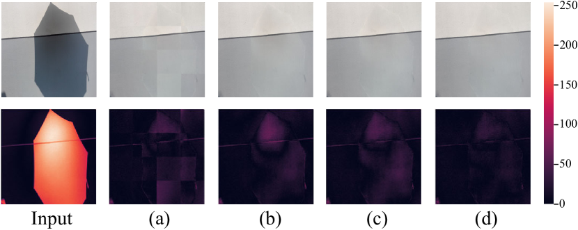
Figure 5: Visual examples of results and error maps for ablation study with different sampling strategies, along with corresponding results from Table 2.

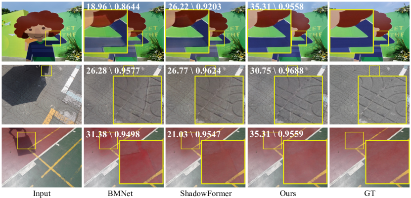
Figure 6: Qualitative comparison with original resolution for BMNet [49], ShadowFormer [14], and ours on ISTD [22] dataset.

Effectiveness of Global-guided Sampling Strategy. Table 2 (e) presents the experiments without overlapping between patches. It turns out significant boundaries between patches in Fig. 5 (a). Second, we established the adaptive noise weights as fixed $W^{d}=1$ in Table 2 (f), which leads to a degradation of the sampling procedure. Reflected in Fig. 5 (b), we can see that there is a large discrepancy between the results and the ground truth. Third, we controlled the noise merge weights solely by the difference between the recovered patch brightness and the recovered global image brightness, i.e., only brightness-based score $S_{\text{bri}}$ exists. The qualitative patch image restored at the beginning of the sampling phase is heavily noisy in Fig. 5 (c). Therefore, it is not accurate to control the weights using brightness alone. The results in Table 2 (g) are inferior to those of our full strategy in Table 2 (h), which considers both the proportion of shaded areas in the patch and the brightness difference between the restored global and local image.

Resolution	Method	PSNR$\uparrow$	SSIM$\uparrow$	RMSE$\downarrow$
original size $640\times 480$	Input Image	20.33	0.874	11.35
	DHAN [4]	27.88	0.921	6.29
	BMNet [49]	29.02	0.928	4.17
	ShadowFormer [14]	30.47	0.935	4.79
	Ours	30.58	0.938	3.69

Table 4: Quantitative results on images with original resolution from ISTD [41].

Effectiveness of RCA module. We assess the impact of the RCA module and the Convolutional Aggregation (CA) at different layers on the ISTD+ [22] dataset.

Table 3 (a) and (b) demonstrate the lower performance when only the RCA module or only the CA module is applied. Table 3 (c) highlights the importance of the RCA module, showing its effectiveness in shallow feature fusion because low-level features capture essential elements, such as edges, colors, and corners, which are crucial for shadow removal tasks. Table 3 (d) confirms that adding the RCA module to both shallow and intermediate layers leads to unsatisfactory results due to limited mask size. Additionally, intermediate layer features primarily capture global semantic information, making them more suitable for fusion using the CA module. Table 3 (e) verifies the overall inferiority of solely incorporating the CA module at each layer compared to the full model in Table 3 (f) with the added RCA module. Therefore, the optimal approach is to apply the RCA module in the initial layer and the CA module in the intermediate layer.

4.4 Extension to Other Image Resolutions

Thanks to the patch-based diffusion modeling approach and the sampling process across overlapping patches during inference, the proposed method enables size-agnostic image restoration. As shown in Fig. 6, our Diff-Shadow maintains excellent illumination consistency even at the original image resolution ($640\times 480$) of the ISTD [22] dataset. Furthermore, as illustrated in Table 4, the proposed Diff-Shadow also achieves state-of-the-art performances. Note that the comparison methods are trained on images of original resolution, while our training is based on images with a resolution of $256\times 256$.

5 Conclusion

In this work, we propose a global-guided diffusion model, named Diff-Shadow, for high-quality shadow removal with no obvious boundaries and consistent illumination. We design a parallel network structure in the framework of the diffusion model to assist in the recovery of local patches using the shadow-free regions from the global image. In addition, we propose a sampling strategy named GSS to further improve the performance of shadow removal during diffusion denoising. Comprehensive experiments demonstrate the superiority of our Diff-shadow. which outperforms the SOTA methods on ISTD, ISTD+, and SRD datasets.

In the appendix, we first provide more implementation details of the proposed Diff-Shadow in Section A. Then, in Section 7, we present some visual results on complex scenes, and more visual comparisons on the ISTD+ [22] and SRD [31] datasets to demonstrate the effectiveness of our approach. Further, Section C discusses some of the limitations of the proposed method.

Appendix A Implementation Details

In all experiments, we employed a consistent network structure as described in Table 5. Our parallel network consists of two UNet structures.

The local and global branches are nearly identical, with the only difference being the absence of a self-attention block in the global branch. The network incorporates six-scale resolutions and includes two residual blocks per-resolution. Detailed configurations and parameters can be found in Table 5.

In the local branch, we perform a channel-wise concatenation of the patch of the shadow image $\tilde{{\mathbf{x}}}^{(i)}$, the variable ${\mathbf{x}_{t}}^{(i)}$, and the mask ${\mathbf{x}_{m}}^{(i)}$, resulting in seven-dimensional input channels (RGB for $\tilde{{\mathbf{x}}}^{(i)}$ and ${\mathbf{x}_{t}}^{(i)}$, and gray channel for ${\mathbf{x}_{m}}^{(i)}$). Additionally, in the global branch, we concatenate the down-sampled full shadow image $\tilde{\mathbf{x}}^{\prime}$ and the mask ${\mathbf{x}_{m}}^{\prime}$, resulting in four-dimensional input image channels. Therefore, our network has a total of eleven input channels.

For the diffusion model, detailed configurations and parameters can be found in Table 6.

Network configurations	Hyper-parameter
input size	64
input channels	11
base channels	128
channel multipliers	1, 1, 2, 2, 4, 4
residual blocks per resolution	2
attention resolution	16 $\times$ 16

Table 5: Network-related configurations and parameter choices.

Diffusion configurations	Hyper-parameter
diffusion steps ($T$)	1000
sampling timesteps ($S$)	25
noise schedule ($\beta_{t}$)	linear: 0.0001 $\rightarrow$ 0.02

Table 6: Diffusion-related configurations and parameter choices.

Appendix B More Visual Examples

Figure 7 presents some visual results on complex scenes to demonstrate the robustness of the proposed method. Figures 8, 9, 10 illustrate some qualitative comparison with DHAN [4], DC-ShadowNet [20], Fu et al. [9], BMNet [49], and ShadowDiffusion [15] on ISTD+ [22] dataset. Our approach clearly outperforms previous methods by preserving the image texture and the luminance consistency. Figure 11 and Figure 12 exhibit some results of the proposed Diff-Shadow on SRD [31] and ISTD [41] datasets, respectively.

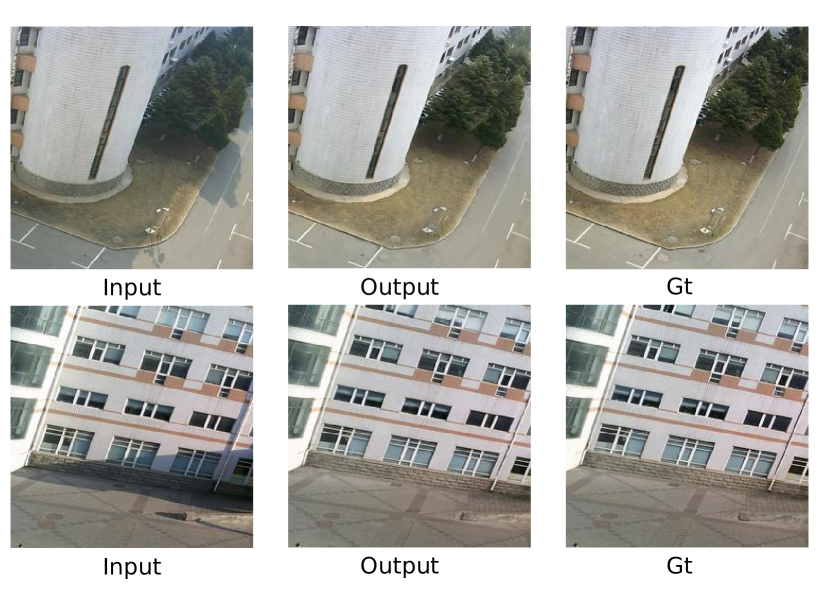
Figure 7: Some visual results on complex scenes.

These results demonstrate the remarkable effectiveness of our approach in removing shadows across diverse scenes due to the incorporation of global information guidance and the powerful modeling capability of the diffusion model for image distribution.

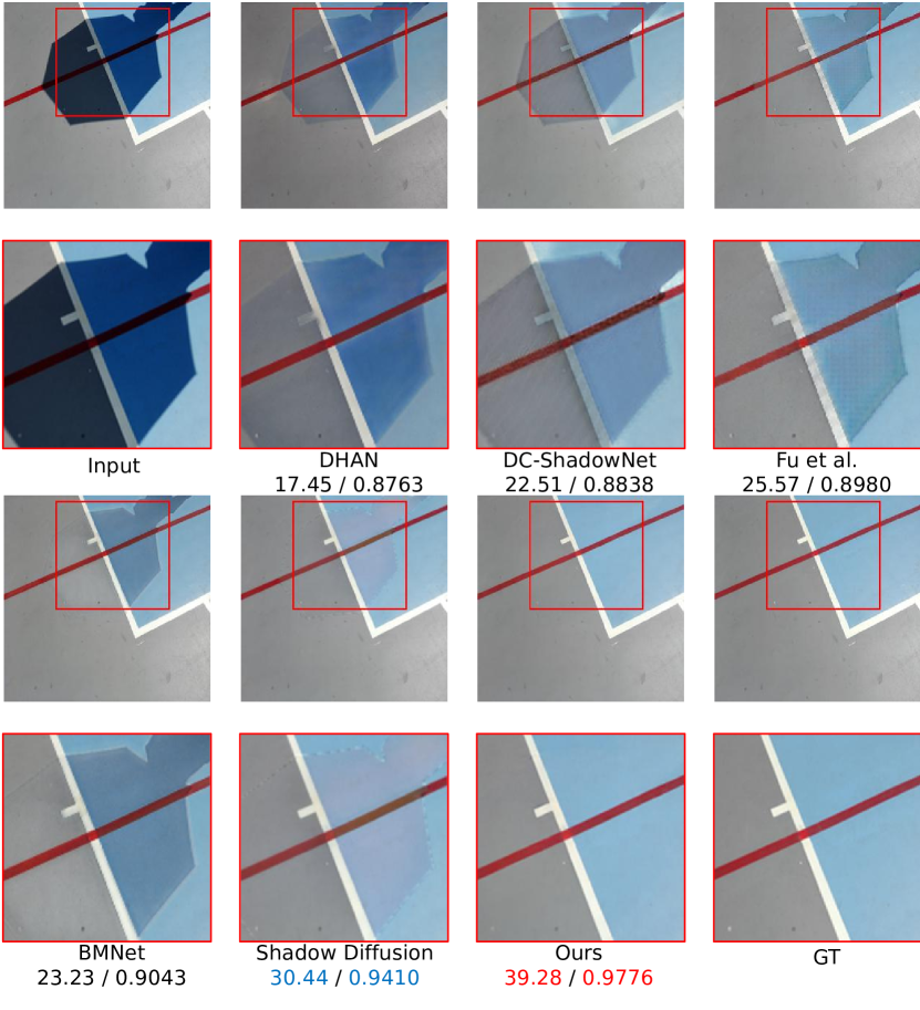
Figure 8: One example of shadow removal results on the ISTD+ [22] dataset. Comparison with DHAN [4], DC-ShadowNet [20], Fu et al. [9], BMNet [49] and ShadowDiffusion [15]. Corresponding values represent the ‘PSNR/SSIM’ scores. The best and second-best results are illustrated in red and blue.

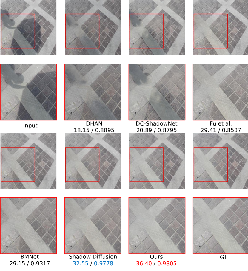
Figure 9: One example of shadow removal results on the ISTD+ [22] dataset. Comparison with DHAN [4], DC-ShadowNet [20], Fu et al. [9], BMNet [49] and ShadowDiffusion [15] on ISTD+ [22] dataset. Corresponding values represent the ‘PSNR/SSIM’ scores. The best and second-best results are illustrated in red and blue.

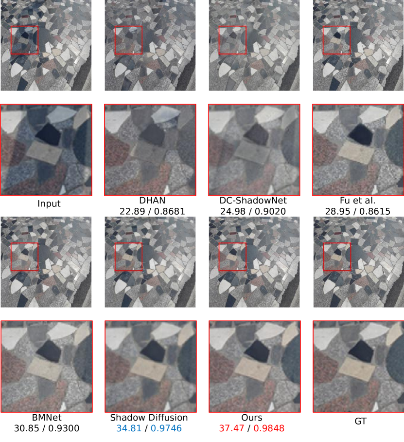
Figure 10: One example of shadow removal results on the ISTD+ [22] dataset. Comparison with DHAN [4], DC-ShadowNet [20], Fu et al. [9], BMNet [49] and ShadowDiffusion [15]. Corresponding values represent the ‘PSNR/SSIM’ scores. The best and second-best results are illustrated in red and blue.

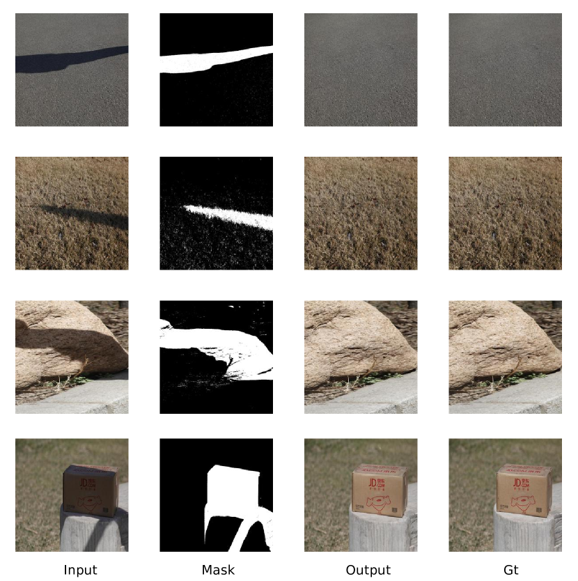
Figure 11: Shadow removal results of Diff-Shadow on the SRD [31] dataset.

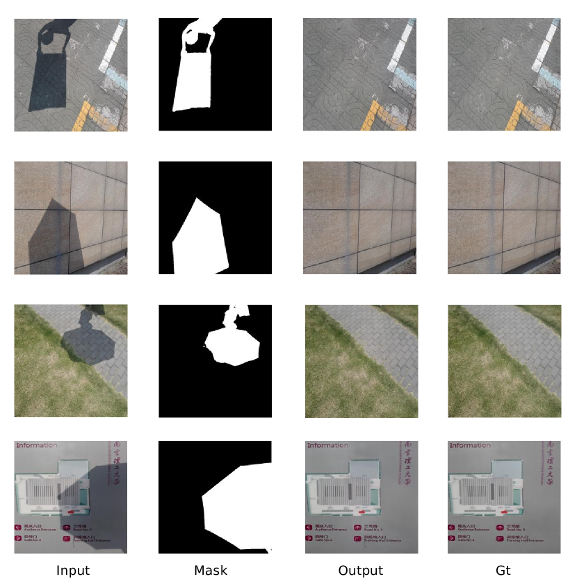
Figure 12: Shadow removal results of Diff-Shadow on the ISTD [41] dataset.

Appendix C Limitations

The main limitation of our approach is the relatively long inference time compared to end-to-end image recovery networks and diffusion methods using simple UNet architectures. Our Diff-Shadow takes 8.72 seconds to recover an image of size $256\times 256$ on a single NVIDIA GTX 2080Ti GPU.

Another natural limitation of our model is the requirement for accurate shadow masks. This enables the network to efficiently use information from the non-shaded portion of the global image, and thus the accuracy of shadow detection directly determines the final result of the shadow removal. Similar to [14, 15, 18], we apply the masks from  [4] for fair comparisons, which is widely used on shadow removal tasks.

References

- Arbel and Hel-Or [2010] Eli Arbel and Hagit Hel-Or. Shadow removal using intensity surfaces and texture anchor points. IEEE TPAMI, 33(6):1202–1216, 2010.
- Chen et al. [2021] Zipei Chen, Chengjiang Long, Ling Zhang, and Chunxia Xiao. Canet: A context-aware network for shadow removal. In ICCV, pages 4743–4752, 2021.
- Chung et al. [2023] Hyungjin Chung, Jeongsol Kim, Sehui Kim, and Jong Chul Ye. Parallel diffusion models of operator and image for blind inverse problems. In CVPR, pages 6059–6069, 2023.
- Cun et al. [2020] Xiaodong Cun, Chi-Man Pun, and Cheng Shi. Towards ghost-free shadow removal via dual hierarchical aggregation network and shadow matting gan. In AAAI, pages 10680–10687, 2020.
- Dhariwal and Nichol [2021] Prafulla Dhariwal and Alexander Nichol. Diffusion models beat gans on image synthesis. NeurIPS, 34:8780–8794, 2021.
- Ding et al. [2023] Zheng Ding, Mengqi Zhang, Jiajun Wu, and Zhuowen Tu. Patched denoising diffusion models for high-resolution image synthesis. arXiv preprint arXiv:2308.01316, 2023.
- Finlayson et al. [2002] Graham D Finlayson, Steven D Hordley, and Mark S Drew. Removing shadows from images. In ECCV, pages 823–836, 2002.
- Finlayson et al. [2005] Graham D Finlayson, Steven D Hordley, Cheng Lu, and Mark S Drew. On the removal of shadows from images. IEEE TPAMI, 28(1):59–68, 2005.
- Fu et al. [2021] Lan Fu, Changqing Zhou, Qing Guo, Felix Juefei-Xu, Hongkai Yu, Wei Feng, Yang Liu, and Song Wang. Auto-exposure fusion for single-image shadow removal. In CVPR, pages 10571–10580, 2021.
- Gao et al. [2023] Sicheng Gao, Xuhui Liu, Bohan Zeng, Sheng Xu, Yanjing Li, Xiaoyan Luo, Jianzhuang Liu, Xiantong Zhen, and Baochang Zhang. Implicit diffusion models for continuous super-resolution. In CVPR, pages 10021–10030, 2023.
- Gryka et al. [2015] Maciej Gryka, Michael Terry, and Gabriel J Brostow. Learning to remove soft shadows. ACM TOG, 34(5):1–15, 2015.
- Guo et al. [2021] Lanqing Guo, Zhiyuan Zha, Saiprasad Ravishankar, and Bihan Wen. Self-convolution: A highly-efficient operator for non-local image restoration. In ICASSP, pages 1860–1864, 2021.
- Guo et al. [2022] Lanqing Guo, Zhiyuan Zha, Saiprasad Ravishankar, and Bihan Wen. Exploiting non-local priors via self-convolution for highly-efficient image restoration. IEEE TIP, 31:1311–1324, 2022.
- Guo et al. [2023a] Lanqing Guo, Siyu Huang, Ding Liu, Hao Cheng, and Bihan Wen. Shadowformer: Global context helps image shadow removal. arXiv preprint arXiv:2302.01650, 2023a.
- Guo et al. [2023b] Lanqing Guo, Chong Wang, Wenhan Yang, Siyu Huang, Yufei Wang, Hanspeter Pfister, and Bihan Wen. Shadowdiffusion: When degradation prior meets diffusion model for shadow removal. In CVPR, pages 14049–14058, 2023b.
- Guo et al. [2012] Ruiqi Guo, Qieyun Dai, and Derek Hoiem. Paired regions for shadow detection and removal. IEEE TPAMI, 35(12):2956–2967, 2012.
- Ho et al. [2020] Jonathan Ho, Ajay Jain, and Pieter Abbeel. Denoising diffusion probabilistic models. NeurIPS, 33:6840–6851, 2020.
- Hu et al. [2019] Xiaowei Hu, Chi-Wing Fu, Lei Zhu, Jing Qin, and Pheng-Ann Heng. Direction-aware spatial context features for shadow detection and removal. IEEE TPAMI, 42(11):2795–2808, 2019.
- Jiang et al. [2023] Hai Jiang, Ao Luo, Songchen Han, Haoqiang Fan, and Shuaicheng Liu. Low-light image enhancement with wavelet-based diffusion models. arXiv preprint arXiv:2306.00306, 2023.
- Jin et al. [2021] Yeying Jin, Aashish Sharma, and Robby T Tan. Dc-shadownet: Single-image hard and soft shadow removal using unsupervised domain-classifier guided network. In ICCV, pages 5027–5036, 2021.
- Kingma and Ba [2015] Diederik P Kingma and Jimmy Ba. Adam: A method for stochastic optimization. In ICLR, 2015.
- Le and Samaras [2019] Hieu Le and Dimitris Samaras. Shadow removal via shadow image decomposition. In ICCV, pages 8578–8587, 2019.
- Le and Samaras [2020] Hieu Le and Dimitris Samaras. From shadow segmentation to shadow removal. In ECCV, pages 264–281, 2020.
- Li et al. [2022] Haoying Li, Yifan Yang, Meng Chang, Shiqi Chen, Huajun Feng, Zhihai Xu, Qi Li, and Yueting Chen. Srdiff: Single image super-resolution with diffusion probabilistic models. Neurocomputing, 479:47–59, 2022.
- Liu and Gleicher [2008] Feng Liu and Michael Gleicher. Texture-consistent shadow removal. In ECCV, pages 437–450. Springer, 2008.
- Lugmayr et al. [2022] Andreas Lugmayr, Martin Danelljan, Andres Romero, Fisher Yu, Radu Timofte, and Luc Van Gool. Repaint: Inpainting using denoising diffusion probabilistic models. In CVPR, pages 11461–11471, 2022.
- Mohan et al. [2007] Ankit Mohan, Jack Tumblin, and Prasun Choudhury. Editing soft shadows in a digital photograph. IEEE Computer Graphics and Applications, 27(2):23–31, 2007.
- Nichol and Dhariwal [2021] Alexander Quinn Nichol and Prafulla Dhariwal. Improved denoising diffusion probabilistic models. In ICML, pages 8162–8171, 2021.
- Niu et al. [2023] Axi Niu, Kang Zhang, Trung X Pham, Jinqiu Sun, Yu Zhu, In So Kweon, and Yanning Zhang. Cdpmsr: Conditional diffusion probabilistic models for single image super-resolution. arXiv preprint arXiv:2302.12831, 2023.
- Özdenizci and Legenstein [2023] Ozan Özdenizci and Robert Legenstein. Restoring vision in adverse weather conditions with patch-based denoising diffusion models. IEEE TPAMI, 2023.
- Qu et al. [2017] Liangqiong Qu, Jiandong Tian, Shengfeng He, Yandong Tang, and Rynson WH Lau. Deshadownet: A multi-context embedding deep network for shadow removal. In CVPR, pages 4067–4075, 2017.
- Rombach et al. [2022] Robin Rombach, Andreas Blattmann, Dominik Lorenz, Patrick Esser, and Björn Ommer. High-resolution image synthesis with latent diffusion models. In CVPR, pages 10684–10695, 2022.
- Saharia et al. [2022a] Chitwan Saharia, William Chan, Huiwen Chang, Chris Lee, Jonathan Ho, Tim Salimans, David Fleet, and Mohammad Norouzi. Palette: Image-to-image diffusion models. In ACM TOG, pages 1–10, 2022a.
- Saharia et al. [2022b] Chitwan Saharia, Jonathan Ho, William Chan, Tim Salimans, David J Fleet, and Mohammad Norouzi. Image super-resolution via iterative refinement. IEEE TPAMI, 45(4):4713–4726, 2022b.
- Shang et al. [2023] Shuyao Shang, Zhengyang Shan, Guangxing Liu, and Jinglin Zhang. Resdiff: Combining cnn and diffusion model for image super-resolution. arXiv preprint arXiv:2303.08714, 2023.
- Song and Ermon [2019] Yang Song and Stefano Ermon. Generative modeling by estimating gradients of the data distribution. NeurIPS, 32, 2019.
- Song and Ermon [2020] Yang Song and Stefano Ermon. Improved techniques for training score-based generative models. NeurIPS, 33:12438–12448, 2020.
- Tian et al. [2023] Chunwei Tian, Menghua Zheng, Wangmeng Zuo, Bob Zhang, Yanning Zhang, and David Zhang. Multi-stage image denoising with the wavelet transform. PR, 134:109050, 2023.
- Vaswani et al. [2017] Ashish Vaswani, Noam Shazeer, Niki Parmar, Jakob Uszkoreit, Llion Jones, Aidan N Gomez, Łukasz Kaiser, and Illia Polosukhin. Attention is all you need. NeurIPS, 30, 2017.
- Wan et al. [2022] Jin Wan, Hui Yin, Zhenyao Wu, Xinyi Wu, Yanting Liu, and Song Wang. Style-guided shadow removal. In European Conference on Computer Vision, pages 361–378. Springer, 2022.
- Wang et al. [2018] Jifeng Wang, Xiang Li, and Jian Yang. Stacked conditional generative adversarial networks for jointly learning shadow detection and shadow removal. In CVPR, pages 1788–1797, 2018.
- Wang et al. [2004] Zhou Wang, Alan C Bovik, Hamid R Sheikh, and Eero P Simoncelli. Image quality assessment: from error visibility to structural similarity. IEEE TIP, 13(4):600–612, 2004.
- Whang et al. [2022] Jay Whang, Mauricio Delbracio, Hossein Talebi, Chitwan Saharia, Alexandros G Dimakis, and Peyman Milanfar. Deblurring via stochastic refinement. In CVPR, pages 16293–16303, 2022.
- Xiao et al. [2013] Chunxia Xiao, Ruiyun She, Donglin Xiao, and Kwan-Liu Ma. Fast shadow removal using adaptive multi-scale illumination transfer. Comput. Graph. Forum, 32(8):207–218, 2013.
- Xie et al. [2023] Yutong Xie, Minne Yuan, Bin Dong, and Quanzheng Li. Diffusion model for generative image denoising. arXiv preprint arXiv:2302.02398, 2023.
- Zhang et al. [2023] Guanhua Zhang, Jiabao Ji, Yang Zhang, Mo Yu, Tommi Jaakkola, and Shiyu Chang. Towards coherent image inpainting using denoising diffusion implicit models. arXiv preprint arXiv:2304.03322, 2023.
- Zhang et al. [2015] Ling Zhang, Qing Zhang, and Chunxia Xiao. Shadow remover: Image shadow removal based on illumination recovering optimization. IEEE TIP, 24(11):4623–4636, 2015.
- Zhang et al. [2020] Ling Zhang, Chengjiang Long, Xiaolong Zhang, and Chunxia Xiao. Ris-gan: Explore residual and illumination with generative adversarial networks for shadow removal. In AAAI, pages 12829–12836, 2020.
- Zhu et al. [2022a] Yurui Zhu, Jie Huang, Xueyang Fu, Feng Zhao, Qibin Sun, and Zheng-Jun Zha. Bijective mapping network for shadow removal. In CVPR, pages 5627–5636, 2022a.
- Zhu et al. [2022b] Yurui Zhu, Zeyu Xiao, Yanchi Fang, Xueyang Fu, Zhiwei Xiong, and Zheng-Jun Zha. Efficient model-driven network for shadow removal. In AAAI, pages 3635–3643, 2022b.