Optimal experimental design:
Formulations and computations

Abstract

Questions of ‘how best to acquire data’ are essential to modeling and prediction in the natural and social sciences, engineering applications, and beyond. Optimal experimental design (OED) formalizes these questions and creates computational methods to answer them. This article presents a systematic survey of modern OED, from its foundations in classical design theory to current research involving OED for complex models. We begin by reviewing criteria used to formulate an OED problem and thus to encode the goal of performing an experiment. We emphasize the flexibility of the Bayesian and decision-theoretic approach, which encompasses information-based criteria that are well-suited to nonlinear and non-Gaussian statistical models. We then discuss methods for estimating or bounding the values of these design criteria; this endeavor can be quite challenging due to strong nonlinearities, high parameter dimension, large per-sample costs, or settings where the model is implicit. A complementary set of computational issues involves optimization methods used to find a design; we discuss such methods in the discrete (combinatorial) setting of observation selection and in settings where an exact design can be continuously parameterized. Finally we present emerging methods for sequential OED that build non-myopic design policies, rather than explicit designs; these methods naturally adapt to the outcomes of past experiments in proposing new experiments, while seeking coordination among all experiments to be performed. Throughout, we highlight important open questions and challenges.

2020 Mathematics Subject Classification: Primary 62-02, 62-08, 62B15, 62K05

Secondary 62L05, 94A17, 65M32

1 Introduction

Acquiring data to inform models and guide decisions is an essential part of scientific inquiry, engineering design, and even policy making. Seldom can we construct a useful model in isolation from data. Rather, data must be used to infer parameters of models, to assess whether models can provide useful predictions, and to spur a wide variety of model improvements. In this setting, it is natural to consider how to acquire data efficiently. Experimental data and field measurements can be costly or time-consuming to acquire; other information sources, similarly, may be expensive to query. Yet we face a multitude of choices in designing such queries. Where to place a sensor? What experimental conditions to impose? What quantity to observe? Do measurements need to be very precise, or would a noisier measurement suffice? When should measurements be made? And how much data should be collected? More broadly, what combination of observations would be most informative or useful—and how should we precisely define notions of ‘informative’ or ‘useful’ in the first place? Crucially, these notions must allow experimental choices to be made before data are acquired.

Optimal experimental design (OED) aims to answer these questions, through mathematical formulations that formalize and tailor them to the ultimate goals of acquiring data. A model developer may have many possible goals, and hence there are many possible criteria for what comprises a good experimental design. Another essential aspect of OED involves numerical algorithms, e.g., for evaluating suitable design criteria, for optimizing over possible experimental configurations, and possibly doing so in a ‘closed-loop’ sequential fashion. Collectively, these endeavors lie at the intersection of many fields: statistical inference and decision theory, information theory, Monte Carlo methods, continuous and combinatorial optimization, dynamic programming and stochastic control, and even reinforcement learning.

Every OED problem has two essential ingredients: an experiment, which is the source of data, and a mathematical model. The role of the model is to simulate what might happen in candidate experiments, and to assess how the results of such experiments might improve the model and its predictions. Formally, the model is a statistical model; in some applications, evaluating this statistical model also involves significant numerical simulation. An underlying presumption of OED is that it is worthwhile to perform many calculations involving the model, in order to plan experiments that are more efficient and effective. These calculations might be far less expensive (by some metric) than performing experiments, or there might be other impediments to experimentation that make finding an optimal design in advance, or building an online optimal design policy for online settings, worth the effort.

The notion of an ‘experiment’ should be construed quite broadly, and certainly not limited to laboratory experiments in the traditional sense. A high-fidelity simulation of a complex model, used to produce data to calibrate the parameters of a simpler model, constitutes an experiment. Arranging a network of sensors, or planning the path of an airborne vehicle carrying instruments, also constitutes designing an experiment. Application domains in which OED is used are similarly vast. OED has long been an essential part of statistical modeling, from the design of clinical trials (Berry et al. 2010) to the design of computer experiments (Sacks et al. 1989); the latter is closely related to the classical problem of design for regression (Elfving 1952, Kiefer and Wolfowitz 1959, Kiefer 1961a). But OED can also be applied to problems involving parameter inference in ordinary or partial differential equations (Huan and Marzouk 2013), to a wide range of inverse problems (Haber et al. 2008, Alexanderian et al. 2016b, Ruthotto et al. 2018, Alexanderian 2021, Helin et al. 2022), and to myriad other ‘complex’ models of data-generating processes—in astronomy (Loredo 2011), systems biology (Liepe et al. 2013), aeroelasticity (Riley et al. 2019), reliability testing (Weaver and Meeker 2021), nuclear physics (Melendez et al. 2021), and beyond.

The evolution of experimental design has a rich and fascinating history. Early twentieth-century approaches to experimental design were motivated by agricultural experiments and similar applications. Statistical methods in this setting often involved hypothesis testing, and a good design was one that maximized the sensitivity of the test. Notable works by Fisher and his collaborators during this period introduced concepts such as balance, orthogonality, blocking, and aliasing (Fisher 1936, Craig and Fisher 1936, Yates 1933, 1937, 1940, Bose 1939, Bose and Nair 1939). Wald recognized that these ideas were relevant to many other fields, and in a seminal paper (Wald 1943) introduced formal notions of the efficiency of a design. With this framework, he was able to explain the success of designs based on Latin squares, commonly used in agricultural experimentation. Following Wald’s work, many core ideas of modern OED emerged towards the middle of the twentieth century (Elfving 1952, Lindley 1956, Kiefer 1958, Stone 1959, Kiefer and Wolfowitz 1959, Kiefer 1959, 1961a), some of them influenced by the emerging discipline of decision theory. Kiefer distinguished various design criteria by giving them meaningful names, and thus originated current ‘alphabetic optimality’ terminology (Kiefer 1958). Much later, Kiefer also showed inter-relationships among various design criteria by introducing more general notions of ‘universal’ optimality (Kiefer 1974). Lindley’s work in the same period (Lindley 1956) aligns more closely with Bayesian statistical thinking, and deserves special mention in light of the current popularity of information theoretic design criteria. These approaches remained largely intractable half a century ago, but with advances in computing power and algorithms, these more general and arguably more rigorous design criteria have become feasible to implement. For a more detailed history of OED, we refer readers to Wynn (1984) and to the texts by Fedorov (1972), Shah and Sinha (1989), and Pukelsheim (2006).

In recent years, interest in OED has expanded from the statistics literature into the uncertainty quantification and applied mathematics communities, where, as noted earlier, an animating goal has been to advance OED methodologies for ‘complex’ models. Here many forms of complexity are relevant: high-dimensional parameters, computationally intensive likelihood functions that involve the evaluation of ordinary or partial differential equations, strong nonlinearity in the dependence of observables on parameters, and the associated non-Gaussianity of posterior distributions in the Bayesian setting. Additional complexities can arise due to data-generating processes that evolve in time, which present the opportunity to design and implement experiments adaptively, i.e., where the results of previous experiments influence the next; this is the setting of sequential optimal experimental design. Another thread relevant to modern OED has come from the computer science literature, where much attention has been paid to the optimization of set functions; methods here underpin a combinatorial approach to OED, where the problem is cast as choosing a subset of a given ‘ground set’ of feasible candidate experiments. And in recent years, tools from machine learning and in particular deep learning have become quite useful for OED, for instance by offering new ways of evaluating complex design criteria in high dimensional, non-Gaussian settings. Of particular interest are expressive machine learning models and learning algorithms for the underlying density (or density ratio) estimation tasks. We will discuss all of these threads, and many more, in the ensuing sections.

We mention here several other excellent surveys that may be of interest to the reader. Steinberg and Hunter (1984) and Pukelsheim (2006) (updated from the original 1993 version) provide comprehensive reviews of non-Bayesian OED for linear models. Ford et al. (1989) discuss design for nonlinear models, while DasGupta (1995) discusses Bayesian designs, mostly for linear models. Atkinson et al. (2007) provide extensive coverage of linear optimal design theory, with some extension to nonlinear and Bayesian methods. The paper of Chaloner and Verdinelli (1995) is an influential review from a statistical perspective, highlighting features of the Bayesian and decision-theoretic approach to OED. We view the Bayesian approach as very natural in the setting of design, and will largely adopt such a perspective here. Clyde (2001) presents an overview of Bayesian OED formulations with various choices of utility.

More recent reviews have placed a greater emphasis on computation. Ryan et al. (2016) discuss Bayesian formulations of OED and then survey computational algorithms for realizing Bayesian designs, emphasizing Monte Carlo methods for estimating design criteria and for searching through design space. Alexanderian (2021) reviews OED for Bayesian inverse problems, emphasizing formulations and algorithms for the infinite-dimensional (function space) setting. Rainforth et al. (2023) provide a survey highlighting recent machine learning and reinforcement learning tools in OED, including sequential design. Strutz and Curtis (2024) present a review of variational OED methodologies and their application to geophysical and in particular seismological problems. There may be other recent reviews of which we are unaware, and we apologize for such omissions.

1.1 Scope and organization of this article

This article aims to provide a broad, comprehensive survey of methodologies for optimal experimental design. Our perspective covers both formulations—i.e., the many ways of posing an OED problem—and computations—i.e., numerical algorithms for finding optimal designs, or tractable approximations of optimal designs, for a range of problem settings. The second topic in particular is multi-faceted—we will draw upon Monte Carlo methods, algorithms for inference and density estimation, and a variety of optimization approaches—but naturally enjoys a close interplay with the first. Our goal is to guide readers who are new to OED from the basic ideas to the research frontier, and to illuminate open issues and challenges at that frontier. Indeed, we believe that the present moment is ripe for a survey of the field: the problems that remain are quite challenging, and a synthesis of ideas and approaches from many different intellectual communities (some of which have been rather disconnected) is needed to make progress.

The article is organized as follows. We begin in Section 2 by describing possible design criteria for OED, each encoding a different notion of what constitutes a ‘good’ experiment. The applicability of these criteria ranges from the rather specific (e.g., linear-Gaussian problems) to the very general. Many are rooted in information-theoretic and/or decision-theoretic formulations. We also mention alternative design heuristics that have been used in practice, and clarify distinctions between the OED problem and several related but different problems, such as Bayesian optimization.

In Section 3 we turn to the first step of computation: numerical algorithms for estimating or bounding the values of these design criteria. We survey Monte Carlo schemes, as well as variational approximations and density estimation methods, for this purpose. Some of these algorithms are applicable to so-called ‘implicit’ Bayesian models, where evaluations of the likelihood function or prior density may be unavailable. We also discuss challenges associated with high-dimensional parameters and data, and dimension reduction schemes that mitigate these challenges. In Section 4 we discuss strategies and algorithms for efficiently optimizing design criteria in various settings. On one hand, we address problems where an exact design of interest is represented by continuous (real-valued) variables. On the other hand, we discuss settings where the design optimization problem is discrete and combinatorial, e.g., a form of subset selection, and continuous relaxations thereof.

Sections 2–4 focus on the all-at-once (‘batch’) design of experiments—that is, ‘fixed’ or static designs that cannot be adjusted as the outcomes of experiments are realized. In contrast, Section 5 turns to the problem of sequential OED, where design decisions are naturally adapted according to the outcomes of previous experiments, while taking into consideration the information to be gained from future experiments. We present sequential OED in a fully Bayesian setting, leveraging the formalism of Markov decision processes. We then highlight recent computational methods for solving this challenging problem, which make use of dynamic programming, various reinforcement learning techniques, and information bounds.

We close in Section 6 with a discussion of open questions and opportunities for future work.

2 Optimal design criteria

We begin by addressing the central question of any OED formulation: In what sense should one deem a candidate design to be ‘good?’ More specifically, by what considerations should one candidate design be deemed better than another? Answering these questions is essential to the notion of optimal design. The answers are formalized by choosing a quantitative design criterion—a function that can then be maximized in order to identify the corresponding optimal design. In this section, we will discuss a wide variety of design criteria and the goals they encode.

To formulate these criteria, we must first specify a statistical model for the observations $Y$ obtained under a candidate design. We need such a model in order to predict the outcomes of candidate experiments, and to relate these outcomes to the ensuing estimation or prediction tasks that motivated the acquisition of data in the first place. We will initially consider parametric statistical models. Any such model is a family of probability distributions for $Y$, indexed by (unknown) model parameters $\theta\in\bm{\Theta}\subseteq\mathbb{R}^{p}$ and by the choice of design $\xi\in\Xi$:

$$\mathcal{M}=\{\textit{{F}}_{Y;\theta,\xi}:\theta\in\bm{\Theta},\ \xi\in\Xi\}.$$ (1)

This model encodes, for any given value of $\theta$ and $\xi$, a complete probabilistic description of the resulting observations, via the cumulative distribution function $\textit{{F}}_{Y;\theta,\xi}$. Further, if every element of $\mathcal{M}$ is absolutely continuous with respect to Lebesgue measure, we can also write the statistical model as a family of conditional probability density functions, i.e., $\mathcal{M}=\{p_{Y|\theta,\xi}(y|\theta,\xi):\theta\in\bm{\Theta},\ \xi\in\Xi\}$. We will make this simplifying assumption from here on, with the understanding that the conditional density of $Y$ could be replaced by a conditional probability measure $\mu(dy|\theta,\xi)$ as needed.

The parameters $\theta$ in the model are unknown and hence the object of estimation or inference. On the other hand, $\xi$ can be controlled by the experimenter. For instance, if candidate $Y$ corresponded to observations of a spatiotemporal process, $\xi$ might represent the spatial and temporal coordinates of a chosen set of observations. In a regression model, $\xi$ encodes the values of the covariates (i.e., independent variables) at which observations are obtained. Different ways of representing $\xi$ will give rise to different optimization problems, which we will discuss in Section 4.

The statistical model immediately yields a likelihood function $\theta\mapsto p_{Y|\theta,\xi}(y|\theta,\xi)$, and the corresponding symmetric, positive semi-definite $p\times p$ Fisher information matrix

$$F(\theta,\xi)\coloneqq\mathbb{E}_{Y|\theta,\xi}[\nabla_{\theta}\log p_{Y|\theta,\xi}(Y|\theta,\xi)\otimes\nabla_{\theta}\log p_{Y|\theta,\xi}(Y|\theta,\xi)],$$ (2)

which is a central object in estimation theory (Lehmann and Casella 1998). Below we will discuss various design criteria based on the Fisher information matrix.

Alternatively, one can take a Bayesian approach and endow the unknown parameters, now denoted as $\Theta$, with a prior distribution. Let this distribution have (Lebesgue) density $p_{\Theta}$ on $\mathbb{R}^{p}$. We will always assume that the prior density is functionally independent of the design $\xi$. The posterior density of $\Theta$ is then given by Bayes’ rule:

$$p_{\Theta|Y,\xi}(\theta|y,\xi)=\frac{p_{Y|\Theta,\xi}(y|\theta,\xi)\,p_{\Theta}(\theta)}{p_{Y|\xi}(y|\xi)}.$$ (3)

In the Bayesian paradigm, the prior and posterior distributions represent, respectively, our states of knowledge before and after having observed $Y=y$. The marginal density of the observations,

$$p_{Y|\xi}(y|\xi)=\int p_{Y|\Theta,\xi}(y|\theta,\xi)\,p_{\Theta}(\theta)\,\mathrm{d}\theta,$$

appearing in the denominator of (3), is called the evidence or marginal likelihood. We will also call this distribution the prior predictive, as it reflects our probabilistic prediction of future values of $Y$ given only the prior on $\Theta$, the statistical model, and a chosen design. Having observed a particular value of the data, say $y^{\ast}$, at some chosen design $\xi$, the posterior predictive density of the data $Y$ for a new design $\xi^{+}$ is

$$p_{Y|\xi^{+},y^{\ast},\xi}(y|\xi^{+},y^{\ast},\xi)=\int p_{Y|\Theta,\xi}(y|\theta,\xi^{+})\,p_{\Theta|Y,\xi}(\theta|y^{\ast},\xi)\,\mathrm{d}\theta.$$

Many design criteria discussed below will explicitly take advantage of this Bayesian formulation of the inference problem. Indeed, we will see that it is useful to have the ability to incorporate prior information on $\Theta$—in general, but especially in nonlinear design settings—and that the Bayesian approach to OED is natural for decision-theoretic reasons as well.

2.1 Design criteria for the linear-Gaussian setting

A rich variety of design criteria, both Bayesian and non-Bayesian, have been developed for linear-Gaussian models. This class of statistical models has numerous practical applications: certainly linear regression, but also linear inverse problems, where observations depend indirectly on the parameters through the action of some linear operator. Canonical linear inverse problems include deconvolution, computerized tomography, and source inversion, among many others (Kaipio and Somersalo 2006). Design criteria in this setting are often quite explicit and tractable, and also serve as a building block for certain nonlinear design approaches.

We specify a general linear-Gaussian model as

$$Y=G\theta+\mathcal{E},$$ (4)

where $G\in\mathbb{R}^{n\times p}$ represents the linear ‘forward’ operator, mapping parameters to data in $\mathbb{R}^{n}$, and $\mathcal{E}$ is a Gaussian random variable with full-rank covariance matrix $\Gamma_{Y|\Theta}\in\mathbb{R}^{n\times n}$ that does not depend on $\theta$. We let $\mathcal{E}$ have mean zero; choosing otherwise would not affect the developments below. In general, both $G$ and $\Gamma_{Y|\Theta}$ can depend on the design $\xi$; that is, we have $G(\xi)$ and $\Gamma_{Y|\Theta}(\xi)$. The linear-Gaussian model can be summarized as $Y|\theta,\xi\,\sim\,\mathcal{N}\left(G(\xi)\theta,\Gamma_{Y|\Theta}(\xi)\right)$.

2.1.1 Classical alphabetic optimality

The Fisher information matrix associated with (4) is

$$F(\theta,\xi)=F(\xi)=G(\xi)^{\top}\Gamma_{Y|\Theta}(\xi)^{-1}G(\xi).$$ (5)

It is thus independent of the value of the parameters $\theta$; this property of linear models greatly simplifies the construction of design criteria. Note also that the inverse of the Fisher information matrix, $F^{-1}$, when it exists, is the covariance of the least-squares estimate and hence the maximum likelihood estimate, $\hat{\theta}(y)$, of $\theta$. Many classical design criteria are therefore chosen to be scalar-valued functionals of the matrix $F$. Indeed, we must somehow ‘scalarize’ $F$ to produce a useful optimization objective, and various scalarizations encode different goals. We recall several of these so-called ‘alphabetic optimality’ criteria as follows.

A-optimal design seeks

$$\xi^{\ast}\in\arg\max_{\xi\in\Xi}\text{tr}\left(F(\xi)\right).$$

When $F$ is invertible, which is invariably the situation of interest in classical design and what we shall assume in the remainder of this subsection, the optimization problem above is equivalent to $\min_{\xi\in\Xi}\text{tr}\left(F^{-1}(\xi)\right)$, which can be interpreted as minimizing the average variance of the $p$ components of $\hat{\theta}$. D-optimal design, similarly, seeks

$$\xi^{\ast}\in\arg\min_{\xi\in\Xi}\log\det\left(F^{-1}(\xi)\right),$$

which minimizes the volume (in $\mathbb{R}^{p}$) of the smallest $100(1-\alpha)\%$ confidence ellipsoid for $\theta$, for any confidence level $1-\alpha$. A useful distinguishing feature of D-optimal designs is that they are invariant under linear reparameterization (and hence rescaling) of $\theta$; that is, if ${\theta}^{\prime}=M\theta$ for some invertible matrix $M$, then a design that is D-optimal for $\theta$ is also D-optimal for $\theta^{\prime}$. This is not true, in general, for other optimality criteria.

While the A- and D-optimality criteria explicitly involve all the eigenvalues of $F$, E-optimal designs minimize the maximum eigenvalue of $F^{-1}(\xi)$, $\lambda_{\text{max}}(F^{-1}(\xi))$ (equivalently, maximize $\lambda_{\text{min}}(F(\xi))=1/\lambda_{\text{max}}(F^{-1}(\xi))$). Such designs thus minimize the variance of $q^{\top}\hat{\theta}$ among all $q\in\mathbb{R}^{p}$ satisfying a norm constraint, that is, they minimize $\max_{\|q\|=w}\mathbb{V}\text{ar}(q^{\top}\hat{\theta})=\max_{\|q\|=w}q^{\top}F(\xi)^{-1}q$ for any $w>0$.

A-, D-, and E-optimality are perhaps the essential building-block design criteria for linear models, but there are numerous others. Some focus on the estimation of a linear combination of the parameters $\theta$, or a subset of the elements of $\theta$. Suppose, for example, that we are primarily interested in $A^{\top}\theta$, where $A\in\mathbb{R}^{p\times s}$, $s<p$, and $A$ has rank $s$. Then $\text{D}_{\text{A}}$-optimality generalizes D-optimality by seeking

$$\xi^{\ast}\in\arg\min_{\xi\in\Xi}\log\det\left(A^{\top}F^{-1}(\xi)A\right).$$ (6)

This objective is justified by noting that $A^{\top}F^{-1}(\xi)A$ is the covariance matrix of $A^{\top}\hat{\theta}$. If we put $A=[I_{s}\ \ 0]^{\top}$, then the design criterion (6) focuses on the first $s$ elements of $\theta$; this is called $\text{D}_{\text{S}}$-optimality.

An analogous generalization of A-optimality, for some matrix $L\in\mathbb{R}^{p\times p}$, is called L-optimality (Atkinson et al. 2007):

$$\xi^{\ast}\in\arg\min_{\xi\in\Xi}\text{tr}(F^{-1}(\xi)L)\,.$$

If $L$ is symmetric and has rank $s\leq p$, then it can be expressed as $L=AA^{\top}$ for $A\in\mathbb{R}^{p\times s}$. Then, using the cyclic property of the trace, the L-optimality objective can be rewritten as $\text{tr}(A^{\top}F^{-1}(\xi)A)$. If $A^{\top}$ is a row vector in this setting (i.e., $s=1$), then the criterion seeks to minimize the variance of a single linear combination of the parameters, and it is called c-optimality.

Other criteria instead seek to control the variance of predictions of the linear model. Consider, specifically, a regression model on some compact domain $\mathcal{X}$, where each row of $G$ is given by the evaluation of a feature vector $f:\mathcal{X}\to\mathbb{R}^{p}$; that is, the $i$th row of $G$ is $G(i,:)=f^{\top}(x_{i})$ for some $x_{i}\in\mathcal{X}$ that is in the support of the design $\xi$. The G-optimality criterion considers the variance of the predicted response at any point $x\in\mathcal{X}$, $f^{\top}(x)F^{-1}(\xi)f(x)$, and seeks a design $\xi$ that will minimize the maximum value of this variance, that is,

$$\xi^{\ast}\in\operatornamewithlimits{argmin}_{\xi\in\Xi}\max_{x\in\mathcal{X}}f^{\top}(x)F^{-1}(\xi)f(x).$$ (7)

Variants of this criterion that target the average variance of the predicted response over a region, rather than its maximum, are called I-optimality or V-optimality. For a much more comprehensive discussion of classical alphabetic optimality criteria and their properties, we refer to Hedayat (1981) and Shah and Sinha (1989) as well as Atkinson et al. (2007, Chapter 10).

We should note here that the assumption of normality on $Y$ is generally not needed for these criteria to apply, and for the statistical interpretations given above to hold. Rather, we need only that $\mathbb{E}[Y]=G\theta$ and $\mathbb{C}\text{ov}(Y)=\Gamma_{Y|\Theta}$. The best linear unbiased estimator still follows from the least squares solution in this setting, and its performance is bounded by the Fisher information matrix (cf. Cramér–Rao bounds). In many situations (including the usual setting for G-optimality described above), it is further assumed that $\Gamma_{Y|\Theta}=\sigma^{2}I$, that is, the observational errors are uncorrelated and have constant variance.

2.1.2 Bayesian alphabetic optimality

In the Bayesian setting, the parameters $\theta$ of the linear model (4) are endowed with a prior distribution. Since these parameters are now modeled as random variables, we write them as uppercase $\Theta$ and require that $\mathcal{E}$ and $\Theta$ be independent. Choosing a conjugate Gaussian prior, $\Theta\sim\mathcal{N}(\mu_{\Theta},\Gamma_{\Theta})$, we obtain a posterior distribution that is again Gaussian; it can be written in closed form as $\Theta|y,\xi\,\sim\mathcal{N}(\mu_{\Theta|Y}(y,\xi),\Gamma_{\Theta|Y}(\xi))$, where

$$\Gamma_{\Theta|Y}(\xi) \coloneqq \left(G(\xi)^{\top}\Gamma_{Y|\Theta}(\xi)^{-1}G(\xi)+\Gamma_{\Theta}^{-1}\right)^{-1}$$ (8)

$$\mu_{\Theta|Y}(y,\xi) \coloneqq \Gamma_{\Theta|Y}(\xi)\left(G(\xi)^{\top}\Gamma_{Y|\Theta}(\xi)^{-1}y+\Gamma_{\Theta}^{-1}\mu_{\Theta}\right).$$ (9)

The posterior mean therefore depends on the realized value of the data $y$, but the posterior covariance matrix does not.

The Bayesian analogue to classical alphabetic optimality uses design criteria that are functions of the posterior covariance matrix. Prior knowledge—and more generally the ‘balance’ of information between the prior and the likelihood, where the latter may be affected by the number of observations—will therefore affect the optimal design, since the design criteria depend on the dispersion (shape and scale) of the posterior.

For instance, Bayesian A-optimality seeks designs that minimize the trace of the posterior covariance matrix,

$$\xi^{\ast}\in\arg\min_{\xi\in\Xi}\text{tr}\left(\Gamma_{\Theta|Y}(\xi)\right)=\text{tr}\left((F(\xi)+\Gamma_{\Theta}^{-1})^{-1}\right).$$

Note that, in contrast with classical A-optimality, this objective no longer requires $F$ to be invertible, as long as the prior covariance $\Gamma_{\Theta}$ is chosen to have full rank. The same is true of all other Bayesian alphabetic optimality criteria, making these criteria well-suited to designs with fewer than $p$ support points, and to ill-posed inverse problems generally (Haber et al. 2008). Bayesian D-optimality seeks to minimize the log-determinant of the posterior covariance matrix,

$$\xi^{\ast}\in\arg\min_{\xi\in\Xi}\log\det\left(\Gamma_{\Theta|Y}(\xi)\right).$$ (10)

Similarly, Bayesian $\text{D}_{\text{A}}$-optimality seeks to minimize the log-determinant of the covariance of the posterior predictive distribution of $A^{\top}\theta$, for some matrix $A\in\mathbb{R}^{p\times s}$ with rank $s<p$; hence the goal is to minimize $\log\det\left(A^{\top}\Gamma_{\Theta|Y}(\xi)A\right)$. See Attia et al. (2018) for an application of this criterion, and of a Bayesian analogue of classical L-optimality. Bayesian E-optimal design minimizes the maximum eigenvalue of $\Gamma_{\Theta|Y}(\xi)$, and so on. For an extensive discussion of Bayesian alphabetic optimality criteria and their interpretations, we refer the reader to Chaloner and Verdinelli (1995) and DasGupta (1995). We will also revisit several of these criteria from the more general viewpoint of decision theory in Section 2.2; the decision-theoretic formulation lets us derive many Bayesian alphabetic optimality criteria from specific utility functions and, crucially, enables generalization to nonlinear models.

In the Bayesian setting, it is also natural to consider linear models with unknown variance parameters, e.g., $\Gamma_{Y|\Theta}=\sigma^{2}I$ with unknown $\sigma^{2}$, and to endow these variance parameters with suitable priors. In general, this extension modifies the optimality criteria discussed above—with some exceptions, such as Bayesian A-optimality using a conjugate inverse Gamma prior for $\sigma^{2}$; for more information, see Chaloner and Verdinelli (1995).

2.1.3 Designs as probability measures

So far, we have deliberately remained somewhat non-specific in describing how the design $\xi$ enters the statistical models (1) or (4), other than to think of $\xi$ as representing all the chosen ‘coordinates’ or locations of the observations on some continuous domain $\mathcal{X}$, or the indices of observations selected from some countable set of candidates. One rather elegant way of formalizing these examples is to cast the design as a probability measure on some domain $\mathcal{X}$. This viewpoint, originating in Kiefer and Wolfowitz (1959), is widely adopted in the classical literature on optimal design.

To explain this perspective, let us first consider the discrete case, where $\mathcal{X}$ is a countable and perhaps finite set of observation indices, $\mathcal{X}=\{1,2,3,\ldots\}$. Suppose that we wish to choose $n$ observations in total. If $n_{i}$ observations are taken at each point $i=1,2,3,\ldots$ and $\sum_{i}n_{i}=n$, then we can write $\xi_{i}=n_{i}/n$ and consider $(\xi_{i})_{i}$ to be a probability measure (Chaloner and Verdinelli 1995). This class of ‘quantized’ measures, with integer $n_{i}$ and hence weights that are multiples of $1/n$, is called an exact design. If each point can only be observed once—i.e., if the selection is without replacement—then we further require $n_{i}\in\{0,1\}$. It is often useful to relax the integer constraint, such that $\xi$ is any probability measure over the set of candidate indices; in this case, $\xi$ is called a continuous or approximate design. Then $\Xi$ is the set of all probability mass functions over $\mathcal{X}$.

Now consider the setting of continuous observation indices, on a compact set $\mathcal{X}\subseteq\mathbb{R}^{d}$, for $d\geq 1$. This setting allows candidate observations to be indexed by some continuous coordinates, e.g., angles for a tomography problem, real-valued spatial coordinates for a sensor placement problem, or any other covariates in a generic regression problem. The notion of a continuous design extends naturally: $\xi$ is simply a probability measure on $\mathcal{X}$, and $\Xi$ is the set of all such probability measures. An exact design here would be a finite mixture of Dirac measures with quantized weights—that is, a measure supported on a finite collection of points in $\mathcal{X}$ with mixture weights that are multiples of $1/n$, i.e., $\xi=\frac{1}{n}\sum_{i=1}^{n}\delta_{x_{i}}$, for $x_{i}\in\mathcal{X}$.

A nice consequence of this general viewpoint is that many quantities relevant to the preceding design criteria can be written as integrals with respect to $\xi$. Consider a linear regression model with features $f:\mathcal{X}\to\mathbb{R}^{p}$ and uncorrelated observational errors. If the design $\xi$ is supported on $n$ equally weighted points $x_{i}\in\mathcal{X}$, $i=1,\ldots,n$, then the Fisher information matrix of the model is

$$F(\xi)=\frac{1}{\sigma^{2}}\sum_{i=1}^{n}f(x_{i})f(x_{i})^{\top}.$$ (11)

This expression follows from (5) by setting

$$G=\left[f(x_{1})^{\top};f(x_{2})^{\top};\ldots;f(x_{n})^{\top}\right]\in\mathbb{R}^{n\times p}$$

and $\Gamma_{Y|\Theta}=\sigma^{2}I_{n}$. If the design has continuous support, then we simply have instead

$$F(\xi)=\frac{n}{\sigma^{2}}\int_{\mathcal{X}}f(x)f(x)^{\top}\xi(\mathrm{d}x),$$

where the $n$ above ensures that the scaling of the integral is consistent with (11).

It is natural to wonder how to reconcile this continuous-support viewpoint with the existence of classical optimal designs supported on a finite set of points in $\mathcal{X}$ (Atwood 1969). In other words, when optimizing some design criterion over the set of all probability measures on the infinite set $\mathcal{X}$, why should a minimizer be supported only on a finite number of locations? In fact, as explained in Atwood (1969) and Kiefer (1961b), under conditions satisfied by any of the design criteria in Section 2.1.1, there exists an optimal design supported on at most $p(p+1)/2$ points. Intuition for the result follows from Carathéodory’s theorem, compactness of $\mathcal{X}$, and the fact that $F$ is a $p\times p$ symmetric matrix: the optimal information matrix $F$ can always be expressed as a convex combination of at most $p(p+1)/2$ rank-one matrices, each produced by a single-point design. The need for $F$ to be full rank, on the other hand, imposes a lower bound of $p$ on the number of points in an optimal design. In the case of Bayesian alphabetic optimality criteria for linear models, similar upper bounds for the number of support points in an optimal design have also been derived (Chaloner 1984). In the nonlinear setting, however, the Fisher information matrix depends on the parameter $\theta$ (see Section 2.1.4). A common approach, discussed below, is then to average a local design criterion over a distribution on $\theta$. Because now (infinitely) many information matrices $F(\theta,\xi)$ are involved, upper bounds on the number of support points do not in general hold (Atkinson et al. 2007, Chaloner and Larntz 1989).

An important theme in classical design theory has been the construction of so-called ‘equivalence theorems’ for continuous designs. The first such result was due to Kiefer and Wolfowitz (1960), who showed that any continuous D-optimal design is also G-optimal, and vice-versa. This result was substantially generalized by Kiefer (1974) and Whittle (1973). The resulting ‘general equivalence theorem’ relies on the fact that the design criteria to be minimized are convex functionals $\phi$ of the probability measure $\xi$. Under this condition, with some further assumptions on the regularity of $\phi$, the equivalence theorem provides multiple equivalent conditions for the optimality of a design $\xi^{\ast}$, some of which correspond to verifying that the directional derivatives of $\phi$ (with respect to feasible designs $\xi$) are zero at $\xi^{\ast}$. The latter are useful to check optimality of a given design measure (in the continuous case), and have been employed in algorithms (Wynn 1972). Variants of the general equivalence theorem have been established for Bayesian alphabetic optimality in linear models (Chaloner 1984, Pilz 1991) and for certain local optimality criteria averaged over the prior in nonlinear models (Chaloner and Larntz 1989). There is a vast array of results along this theme, which we will not attempt to survey here. Instead we refer the reader to the comprehensive framework in Pukelsheim (2006), which tackles design optimality for linear models using tools of convex analysis, and the historical perspective in Wynn (1984).

Since our interest is largely in nonlinear problems (as well as infinite-dimensional linear problems), we will generally resort to numerical methods for optimizing $\xi$, which must in any case employ tractable finite-dimensional parameterizations of candidate designs. Moreover, only an exact design can be realized in an experiment, and hence some notion of ‘rounding’ is usually needed if a problem is initially solved from a continuous design perspective. We will discuss these considerations further in Section 4.

2.1.4 Challenges of nonlinear design

In problems where dependence on the model parameters $\theta$ is nonlinear, the Fisher information matrix $F$ will generally vary with $\theta$. Since $\theta$ is unknown, it is then unclear where to evaluate $F(\theta,\xi)$ and any of the associated design criteria.

A relatively crude approach is simply to choose some reference or ‘best-guess’ parameter value $\theta_{0}$ and proceed; this is known as ‘local’ design, but it clearly ignores parameter uncertainty and the impact of nonlinearity, and may have sharp dependence on the choice of $\theta_{0}$. One could iterate this approach, by estimating $\theta$ after collecting data from a first local design, and then using the estimated parameter value to produce a new local design, and so on (Korkel et al. 1999). A more principled alternative is a minimax formulation (Fedorov and Hackl 1997, King and Wong 2000, Berger and Wong 2009). If $\phi(\theta,\xi)$ is any ‘local’ design criterion (containing the parameter-dependent Fisher information matrix $F(\theta,\xi)$, for instance, $\phi(\theta,\xi)=\log\det F^{-1}(\theta,\xi)$), then we seek

$$\xi^{\ast}\in\operatornamewithlimits{argmin}_{\xi\in\Xi}\max_{\theta\in\bm{\Theta}}\phi(\theta,\xi).$$

An interpretation of this objective is that it seeks the design with best performance for the worst-case parameter value, i.e., the value of $\theta$ that is most challenging to estimate (in the sense of $\phi$). This idea has been explored by Sun and Yeh (2007) and Siade et al. (2017), among others, but generally leads to a rather difficult optimization problem. Typically $\phi$ is chosen to be a classical alphabetic optimality criterion (as in the example of D-optimality above), and thus the only ‘prior’ information on $\theta$ in these formulations is via the set $\bm{\Theta}$.

Another natural alternative is to introduce a prior distribution $p_{\Theta}$ for $\theta$ and to average any local design criterion $\phi(\theta,\xi)$ over this prior. This approach is widely adopted, due in no small part to its computational tractability; see Pronzato and Walter (1985) and Fedorov and Hackl (1997). If $\phi$ is solely based on the Fisher information, however, then such a formulation is only ‘pseudo-Bayesian’ (Atkinson et al. 2007, Ryan et al. 2016). Indeed, in some such works, the prior is used as a means of handling the parameter dependence arising from nonlinearity but then discarded for subsequent analysis. Ryan et al. (2016) argue that any ‘fully Bayesian’ design criterion must be a functional of the posterior distribution. Interestingly, however, Walker (2016) shows that prior expectation of the trace of the Fisher information matrix,

$$\int\text{tr}(F(\theta,\xi))p_{\Theta}(\theta)\,\mathrm{d}\theta,$$

has an information-theoretic interpretation. Overstall (2022) and Prangle et al. (2023) both explore using this quantity as a design criterion in nonlinear problems, and show that it has a decision-theoretic justification as well.

As a step in the ‘fully Bayesian’ direction, given a nonlinear model and a Gaussian prior $p_{\Theta}$ with full rank covariance matrix $\Gamma_{\Theta}$, one could seek, as proposed in Chaloner and Verdinelli (1995),

$$\xi^{\ast}\in\arg\max_{\xi\in\Xi}\int\log\det\left(F(\theta,\xi)+\Gamma_{\Theta}^{-1}\right)p_{\Theta}(\theta)\,\mathrm{d}\theta.$$ (12)

This can be loosely interpreted as minimizing the average, over the prior predictive distribution of $Y$, of the log-determinant of the covariance of a Gaussian approximation of each resulting posterior. Yet this interpretation is rather imprecise, as for a general nonlinear model, $F(\theta^{\prime},\xi)+\Gamma_{\Theta}^{-1}$ can be very far from the precision matrix of the posterior distribution that results from a realization of the data $y\sim p_{Y|\theta,\xi}(\cdot|\theta^{\prime},\xi)$. Criteria such as this are best viewed as approximations of an expected utility function arising from a more principled decision-theoretic formulation, which we discuss next.

2.2 Decision- and information-theoretic formulations

The decision-theoretic approach to OED was formalized by Lindley (1956) (see also Stone 1959, Raiffa and Schlaifer 1961) and has two primary ingredients: a utility function $u$, chosen to reflect the purpose of the experiment; and the Bayesian principle of averaging over what is uncertain (Berger 1985). In this framework, any design criterion takes the form of an expected utility, to be maximized with respect to $\xi$:

$$U(\xi)=\mathbb{E}_{Y,\Theta|\xi}[u(\xi,Y,\Theta)]=\iint p(y,\theta|\xi)\,u(\xi,y,\theta)\,\mathrm{d}\theta\,\mathrm{d}y.$$ (13)

Here, the utility function $u(\xi,y,\theta)$ quantifies the value of an experiment performed with a design $\xi$ that yields observations $y$, if the true parameter value is $\theta$. Since the outcome of the experiment is not known when selecting $\xi$, and since the parameter value is also uncertain, we average over the joint prior distribution of $Y$ and $\Theta$. This process yields the expected utility $U(\xi)$. Many choices of utility function $u$ have been proposed and explored in the literature. We review some of the possibilities below.

2.2.1 Expected information gain in parameters

The influential paper of Lindley (1956) proposed using the expected gain in Shannon information, from prior to posterior, as an optimal experimental design criterion. It is evocative to think of this quantity in at least two ways, namely

$$U_{\text{KL}}(\xi) =\mathbb{E}_{Y|\xi}\left[D_{\text{KL}}(p_{\Theta|Y,\xi}||p_{\Theta})\right]$$ (14)

$$=H(\Theta)-H(\Theta|Y,\xi)$$ (15)

where $D_{\text{KL}}$ denotes the Kullback–Leibler (KL) divergence, or relative entropy, from prior to posterior,

$$D_{\text{KL}}(p_{\Theta|y,\xi}||p_{\Theta})=\int p(\theta|y,\xi)\log\frac{p(\theta|y,\xi)}{p(\theta)}\,\mathrm{d}\theta,$$ (16)

and the two terms in (15) are the entropy and conditional entropy, respectively:

$$H(\Theta) =-\int p(\theta)\log p(\theta)\,\mathrm{d}\theta,$$ (17)

$$H(\Theta|Y,\xi) =-\iint p(y,\theta|\xi)\log p(\theta|y,\xi)\,\mathrm{d}\theta\,\mathrm{d}y.$$ (18)

Equality of the expressions (14) and (15) is easily verified. Note that $U_{\text{KL}}$ is always non-negative: conditioning reduces entropy on average (not necessarily for each realization $Y=y$, but when averaging over values of $y$), with zero entropy reduction $H(\Theta)=H(\Theta|Y,\xi)$ if and only if $\Theta$ and $Y|\xi$ are independent. Similarly the KL divergence, whose expectation yields (14), is always non-negative and reaches zero if and only if the two distributions being compared are identical (Cover and Thomas 2006). Some intuition for maximizing this criterion is that the design $\xi$ yielding data $Y$ that most reduce Shannon entropy is, in this information-theoretic sense, the most informative. Another intuition is that an optimal experiment should maximize the ‘change’ (here, quantified by the KL divergence) from the prior to the posterior, averaged over the prior predictive distribution of the data $Y$.

Lindley’s original rationale for the design criterion $U_{\text{KL}}$ was not rooted in decision theory, but the criterion was later given a decision-theoretic justification by Bernardo (1979); see also the discussion in Prangle et al. (2023). Bernardo frames the task of inference as a decision problem, where making a decision amounts to returning a probability density function for the parameters of interest $\Theta$. He argues that the utility function for this decision should be a proper, local scoring rule (Gneiting and Raftery 2007), and that these desiderata in turn dictate that $u$ must specifically be a logarithmic scoring rule. In the language of (13) above, this means that one should choose

$$u^{\text{score}}(\xi,y,\theta)=\log p(\theta|y,\xi)-\log p(\theta).$$ (19)

Substituting this utility into (13) immediately yields (14) and (15).

Note also that choosing the utility to be the KL divergence from prior to posterior, which depends explicitly on $y$ and $\xi$ but not on $\theta$,

$$u^{\text{div}}(\xi,y,\theta)=D_{\text{KL}}(p_{\Theta|y,\xi}||p_{\Theta})=u^{\text{div}}(\xi,y)$$ (20)

and substituting this utility into (13), yields the same expected utility $U_{\text{KL}}$ (14). We also call $U_{\text{KL}}$ the expected information gain (EIG) in $\Theta$, from prior to posterior. It is useful for subsequent computations (see Section 3) to write the EIG more explicitly as follows:

$$U_{\text{KL}}(\xi) =\iint p(y,\theta|\xi)\log\frac{p(\theta|y,\xi)}{p(\theta)}\,\mathrm{d}\theta\,\mathrm{d}y$$ (21)

$$=\iint p(y,\theta|\xi)\log\frac{p(y|\theta,\xi)}{p(y|\xi)}\,\mathrm{d}\theta\,\mathrm{d}y$$ (22)

$$=\iint p(y,\theta|\xi)\log\frac{p(y,\theta|\xi)}{p(y|\xi)p(\theta)}\,\mathrm{d}\theta\,\mathrm{d}y$$ (23)

$$\eqqcolon\mathcal{I}(Y;\Theta|\xi).$$

In all of these expressions, the joint prior predictive density of $Y$ and $\Theta$ can be factored as $p(y,\theta|\xi)=p(y|\theta,\xi)p(\theta)$, i.e., as a product of likelihood and prior. Moving from (21) to (22) is an application of Bayes’ rule (3). Both (21) and (22) make clear that some kind of posterior calculation is necessary: the former involves the normalized posterior density $p(\theta|y,\xi)$, while the latter involves the posterior normalizing constant $p(y|\xi)$. Moreover, these expressions must be evaluated for a range of $y$ values—i.e., for ‘all possible’ posterior distributions—via the outer expectation. The last expression above, (23), shows that EIG is equivalent to the mutual information (MI) between the parameters and observations given the design, $\mathcal{I}(Y;\Theta|\xi)$. Henceforth, we will use the terms EIG and MI interchangeably.

Expanding (22) into two terms also shows that the EIG is a difference of entropies of the data, paralleling (15),

$$U_{\text{KL}}(\xi) =H(Y|\xi)-H(Y|\Theta,\xi).$$ (24)

For some statistical models, $H(Y|\Theta,\xi)$ is a constant function of $\xi$. One example is the case of a nonlinear model with additive noise, $Y=G(\Theta,\xi)+\mathcal{E}$, where $\mathcal{E}$ is independent of $\Theta$ and its distribution does not depend on $\xi$; then the entropy $H(Y|\Theta=\theta,\xi)=H(\mathcal{E})$ and hence does not depend on $\theta$ or $\xi$. Maximizing EIG then specializes to maximizing the entropy of the prior marginal distribution of $Y$. This design strategy is called ‘maximum entropy sampling’; see Shewry and Wynn (1987) and Sebastiani and Wynn (2000).

The EIG objective has additional desirable properties. For one, it is invariant under bijective transformations of $\theta$; this property follows from the invariance of the KL divergence to such transformations, and thus includes rescalings of the parameters as well as more complex reparameterizations. We also emphasize that there are no assumptions of linearity or Gaussianity in the motivation for the EIG objective, and in any of its expressions above.

In the linear-Gaussian case, however, maximizing EIG is equivalent to seeking a Bayesian D-optimal design (10). To see this, note that when $\Theta$ and $Y|\xi$ are jointly Gaussian (as in Section 2.1.2), the EIG or MI can be written in closed form as

$$\mathcal{I}(Y;\Theta|\xi) =\frac{1}{2}\left(\log\det\Gamma_{\Theta}-\log\det\Gamma_{\Theta|Y}(\xi)\right)$$ (25)

$$=\frac{1}{2}\left(\log\det\Gamma_{Y}(\xi)-\log\det\Gamma_{Y|\Theta}(\xi)\right),$$ (26)

where $\Gamma_{Y}$ is the marginal (prior predictive) covariance of $Y$,

$$\Gamma_{Y}(\xi)=G(\xi)\Gamma_{\Theta}G(\xi)^{\top}+\Gamma_{Y|\Theta}(\xi).$$

From (25), it is apparent that maximizing EIG with respect to $\xi$ is equivalent to minimizing the log-determinant of the posterior covariance. If, additionally, the observational error covariance is independent of the design, then $\Gamma_{Y|\Theta}(\xi)=\Gamma_{Y|\Theta}$ and an equivalent goal, via (26), is to maximize the log-determinant of the marginal covariance $\Gamma_{Y}$; this is a specific (linear-Gaussian) case of the maximum entropy sampling described above.

It is interesting to note that the Bayesian D-optimality criterion for linear-Gaussian models can be derived from other utility functions, besides (19) and (20); see Chaloner and Verdinelli (1995, Section 2.2) for details.

2.2.2 Other utility functions

Having defined an information- and decision-theoretic design criterion for inference of the model parameters $\Theta$, it is natural to extend this construction to other goals.

Suppose that we are interested in only a subset of the model parameters. Partitioning $\Theta$ as $\Theta=(\Theta_{1},\Theta_{2})$, information gain in $\Theta_{1}$ is captured by the KL divergence from its prior marginal distribution to its posterior marginal distribution:

$$u(\xi,y) =D_{\text{KL}}(p_{\Theta_{1}|y,\xi}||p_{\Theta_{1}}),$$ (27)

where

$$p(\theta_{1})=\int p(\theta_{1},\theta_{2})\,\mathrm{d}\theta_{2}\ \ \ \text{and}\ \ \ p(\theta_{1}|y,\xi)=\int p(\theta_{1},\theta_{2}|y,\xi)\,\mathrm{d}\theta_{2}.$$

The outer expectation over $Y$ in (13), yielding the expected information gain in $\Theta_{1}$, must still account for uncertainty in both blocks of $\Theta$. The optimal design criterion in this case becomes

$$U(\xi) =\iiint p(y|\theta_{1},\theta_{2},\xi)p(\theta_{1},\theta_{2})\,\log\frac{p(\theta_{1}|y,\xi)}{p(\theta_{1})}\,\mathrm{d}\theta_{1}\,\mathrm{d}\theta_{2}\,\mathrm{d}y$$ (28)

$$=\iiint p(y|\theta_{1},\theta_{2},\xi)p(\theta_{1},\theta_{2})\,\log\frac{p(y|\theta_{1},\xi)}{p(y|\xi)}\,\mathrm{d}\theta_{1}\,\mathrm{d}\theta_{2}\,\mathrm{d}y.$$ (29)

The second expression is analogous to (22) in that it uses densities for the data $Y$, but now even the numerator of the density ratio involves marginalization, as

$$p(y|\theta_{1},\xi) =\int p(y|\theta_{1},\theta_{2},\xi)p(\theta_{2}|\theta_{1})\,\mathrm{d}\theta_{2}.$$ (30)

Compared to the EIG in $\Theta$, evaluating this objective therefore requires an additional integration over $\Theta_{2}$. Note also that (28) and (29) are equivalent to the MI, $\mathcal{I}(Y;\Theta_{1}|\xi)$. In this formulation, $\Theta_{2}$ could represent a variety of possible ‘nuisance’ parameters in the statistical model, i.e., any parameters that are uncertain but simply not the modeler’s immediate object of interest (Feng and Marzouk 2019, Alexanderian et al. 2021). Special examples include the parameters of a discrepancy model (Kennedy and O’Hagan 2001) designed to capture model error, or the background medium in an inverse scattering problem (Borges and Biros 2018).

A generalization of the preceding formulation is to consider the EIG in some (generally nonlinear) function of the parameters $\Theta$, $Z=\Psi(\Theta)$, where $\Psi:\bm{\Theta}\to\mathbb{R}^{q}$ for some $q\leq p$. This can be thought of as a ‘goal-oriented’ objective (just like Bayesian $\text{D}_{\text{A}}$-optimality in the linear-Gaussian case) where the function $\Psi$ encodes the true quantity of interest. Now we seek to maximize the expected KL divergence from the prior predictive distribution of $Z$ to its posterior predictive distribution:

$$U(\xi) =\mathbb{E}_{Y|\xi}\left[D_{\text{KL}}(p_{Z|Y,\xi}||p_{Z})\right]$$

$$=\iint p(y,z|\xi)\,\log\frac{p(z|y,\xi)}{p(z)}\,\mathrm{d}z\,\mathrm{d}y$$ (31)

$$=\iint p(y,z|\xi)\,\log\frac{p(y|z,\xi)}{p(y|\xi)}\,\mathrm{d}z\,\mathrm{d}y$$ (32)

$$=\mathcal{I}(Y;Z|\xi).$$

Notably, this objective is also the original object of interest in Bernardo (1979). While it is straightforward to write down, it raises significant computational challenges, beyond those associated with calculating EIG in the parameters alone. For generic $\Psi$, $p(\theta)$, and $p(y|\theta,\xi)$, we do not have simple expressions for the prior density $p(z)$ or the posterior density $p(z|y,\xi)$ of $Z$ (even up to a normalizing constant) appearing in (31). Nor do we have easy access to the marginal likelihood $p(y|z,\xi)$ to instead evaluate (32). Numerical approximations are needed, involving density estimation or approximate Bayesian computation; see Section 3. Of course, in specific cases (such as linear $\Psi$ with Gaussian priors) some aspects of the expressions above become more tractable. We note also that if $\Psi$ is bijective, then EIG in $Z$ is identical to EIG in $\Theta$, since (as noted earlier) the information gain objective is invariant under bijective transformations; otherwise the EIG in $Z$ is smaller (Bernardo 1979, Theorem 1).

The optimal design obtained by maximizing the EIG in some $Z$ can differ drastically from the design maximizing EIG in $\Theta$. Figure 2.1 illustrates these contrasts for sensor placement in a time-dependent advection-diffusion problem (Zhong et al. 2024). The parameter $\Theta$ is the unknown source location, endowed with a uniform prior on $[0,1]^{2}$. The source emits a scalar quantity that diffuses and is advected towards the top-right of the $[0,1]^{2}$ domain, with the advection velocity increasing linearly in time, from a value of zero at $t=0$. The design entails placing a single sensor, with coordinates $\xi=(\xi_{1},\xi_{2})\in[0,1]^{2}$, that measures the concentration of the scalar at time $t_{1}>0$. Figure 2.1LABEL:sub@f:KL_nonGOOED shows a map of EIG in $\Theta$ as function of sensor location (estimated numerically; see Section 3). We see that the optimal measurement location is not unique, but lies roughly 0.2 units of distance from the center of the domain; the slight asymmetry is due to the direction of advection. Figure 2.1LABEL:sub@f:KL_GOOED, in contrast, shows maps of EIG for four different choices of $Z$; each $Z$ is the predicted concentration of the passive scalar at a future time $t_{2}>t_{1}$ and at the specific location marked by a red star in each panel. We see that the optimal sensor locations, maximizing these goal-oriented EIG criteria, are markedly different from those in Figure 2.1LABEL:sub@f:KL_nonGOOED.

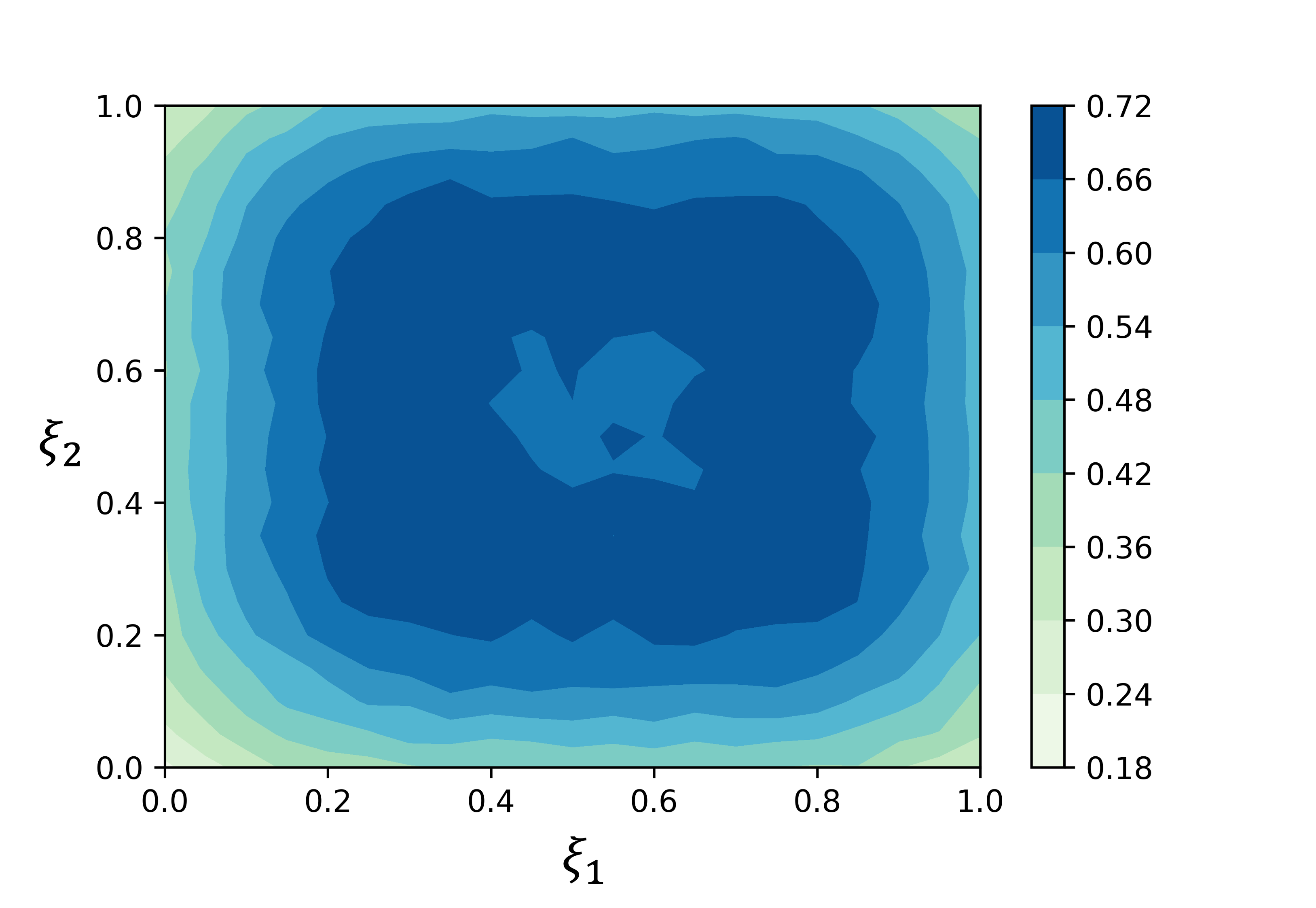
(a) EIG in $\Theta$

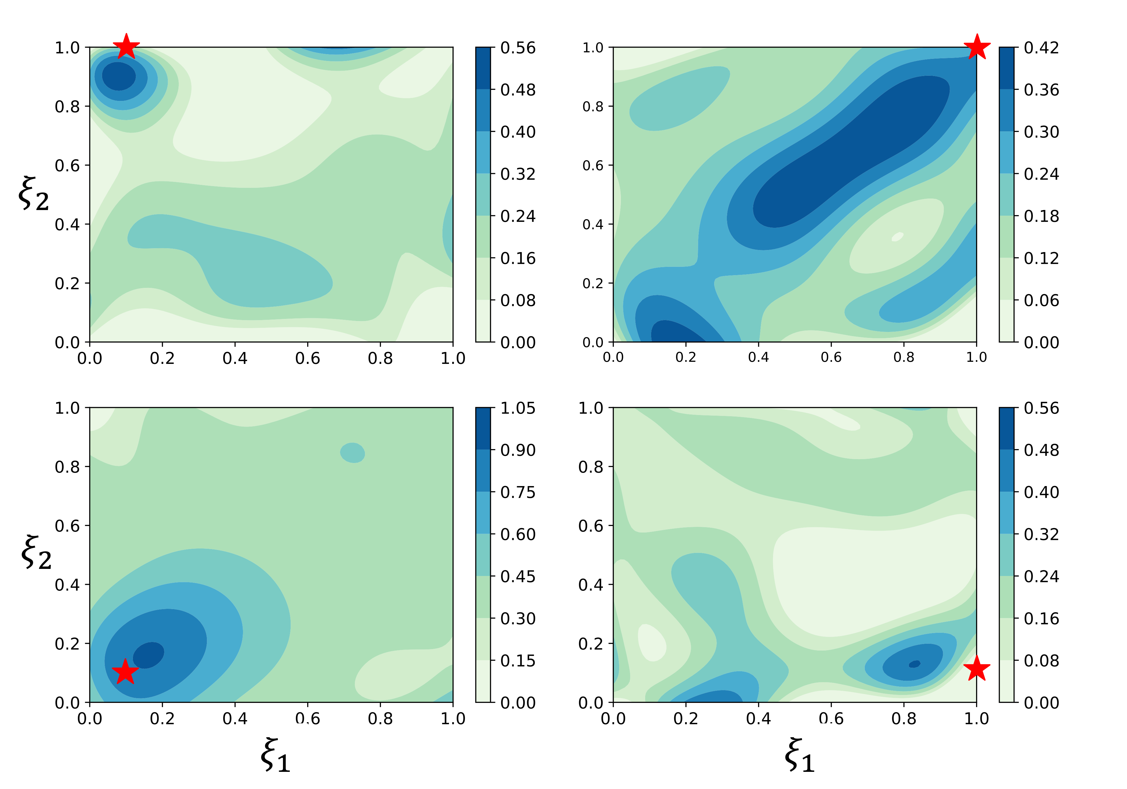
(b) EIG in various $Z$

Figure 2.1: Optimal sensor placement in a time-dependent advection-diffusion problem. Each figure shows a map of expected information gain (EIG) in a chosen quantity, as a function of the sensor location $\xi\in[0,1]^{2}$. Measurements are made at time $t_{1}>0$, and advection is towards the top right. (a) EIG in the unknown source location $\Theta$. (b) EIG for different quantities of interest $Z$, where each $Z$ is the predicted concentration at some future time $t_{2}>t_{1}$, at the location marked by the red star. The optimal designs, maximizing EIG in each case, differ significantly.

If the quantity of interest $Z$ is random given $\theta$, e.g., if it is described by a conditional density $p(z|\theta)$, then the formulation above still applies. Computations may actually be easier: the problem of estimating $p(z)$ or $p(z|y,\xi)$ is smoothed by the kernel $p(z|\theta)$, and the restriction that $q\leq p$ is lifted as long as the conditional density $p(z|\theta)$ on $\mathbb{R}^{q}$ exists. A special case is when $Z=Y|\xi^{+}$, that is, we wish to maximize information gain in the model prediction for some given design $\xi^{+}$. We call this future prediction $Y^{+}$, to distinguish it from the potential outcomes $Y$ of the experiment being currently designed. In this case, the utility $u$ can be set to

$$u(\xi,y) =D_{\text{KL}}(p_{Y^{+}|y,\xi,\xi^{+}}||p_{Y^{+}|\xi^{+}}),$$ (33)

which yields, as an expected utility, the expected information gain in $Y^{+}$:

$$U(\xi) =\iint p(y,y^{+}|\xi,\xi^{+})\,\log\frac{p(y^{+}|y,\xi,\xi^{+})}{p(y^{+}|\xi^{+})}\,\mathrm{d}y^{+}\,\mathrm{d}y$$ (34)

$$=\iiint p(y|\theta,\xi)p(y^{+}|\theta,\xi^{+})p(\theta)\,\log\frac{p(y^{+}|y,\xi,\xi^{+})}{p(y^{+}|\xi^{+})}\,\mathrm{d}y^{+}\,\mathrm{d}y\,\mathrm{d}\theta$$ (35)

$$=\mathcal{I}(Y;Y^{+}|\xi,\xi^{+}).$$ (36)

The penultimate line above reflects the fact that $Y$ and $Y^{+}$ are conditionally independent given $\theta$, and hence their joint prior predictive can be expanded and factored by introducing the parameter $\theta$ explicitly.

A final information-theoretic utility that we will consider arises from problems of model discrimination in the Bayesian setting (Myung and Pitt 2009). Suppose we have a countable set of models $\mathcal{M}_{m}$, $m=1,2,\ldots$, each with its own parameters, $\theta_{m}\in\bm{\Theta}_{m}\subseteq\mathbb{R}^{p_{m}}$, and its own prior on parameters, $p(\theta_{m})$. Suppose there is also a (discrete) prior distribution over the model indicators $m$. As a utility, we choose the relative entropy from this prior to the posterior distribution over model indicators,

$$u(\xi,y)=\sum_{m}P(m|y,\xi)\log\frac{P(m|y,\xi)}{P(m)}.$$ (37)

Following (13), we must take an expectation over the prior predictive distribution of $Y$ to obtain an expected utility. Now, however, because there are multiple possible models, the prior predictive distribution is itself a mixture of the prior predictives of each model:

$$p(y|\xi)=\sum_{m}P(m)p(y|m,\xi)=\sum_{m}P(m)\int_{\bm{\Theta}_{m}}p(y|\theta_{m},\xi)p(\theta_{m})\,\mathrm{d}\theta_{m},$$ (38)

where conditioning on $\theta_{m}$ also implies conditioning on $m$ at the same time. The EIG in the model indicator $m$ follows by combining (37) and (38): $U(\xi)=\int u(\xi,y)p(y|\xi)\,\mathrm{d}y$. As noted in Ryan et al. (2016), this design approach applies in the $\mathcal{M}$-closed framework for model selection (see Bernardo and Smith 2000, Chapter 6); that is, the true (data-generating) model is assumed to be within the set of models considered, and one must assign a prior weight $P(m)$ to the event that each model is true. Examples of Bayesian OED for model discrimination can be found in Myung and Pitt (2009), Cavagnaro et al. (2010), McGree et al. (2012), Drovandi et al. (2014), Aggarwal et al. (2016), and Hainy et al. (2022).

While most of the preceding discussion has focused on information-theoretic utilities, the decision-theoretic framework described at the start of Section 2.2 is certainly not limited to utility functions of this kind. As described in Ryan et al. (2016) and Chaloner and Verdinelli (1995), another natural utility is a quadratic loss, motivated by the desire to extract a point estimate of $\theta$ from the posterior. For instance, let $\bar{\theta}(y,\xi)\coloneqq\mathbb{E}[\Theta|y,\xi]$ denote the posterior mean. Then we can write

$$u(\xi,y,\theta)=-\left(\theta-\bar{\theta}(y,\xi)\right)^{\top}B\left(\theta-\bar{\theta}(y,\xi)\right)$$ (39)

for some symmetric positive semi-definite matrix $B\in\mathbb{R}^{p\times p}$. The expected utility is then

$$U(\xi)=-\iint\left(\theta-\bar{\theta}(y,\xi)\right)^{\top}B\left(\theta-\bar{\theta}(y,\xi)\right)p(y,\theta|\xi)\,\mathrm{d}\theta\,\mathrm{d}y,$$ (40)

which is the negative Bayes risk of the posterior mean under a weighted squared error loss. Maximizing the expected utility over $\xi$ thus minimizes this risk. As noted in Chaloner and Verdinelli (1995), in the case of a linear-Gaussian model, this formulation reverts to Bayesian A-optimal design with weight matrix $B$, i.e., $\min_{\xi}\text{tr}\left(B\,\Gamma_{\Theta|Y}(\xi)\right)$.

Another family of non-information-theoretic utilities involves scalar functionals of the posterior covariance matrix; these are not strictly motivated by point estimation, but rather can be seen as a more computationally tractable alternative to information-theoretic utilities that require calculation of posterior normalizing constants. Ryan et al. (2016) specifically suggest using as a utility the determinant of the posterior precision matrix:

$$u(\xi,y)=\frac{1}{\det\left(\mathbb{C}\text{ov}(\Theta|y,\xi)\right)}$$ (41)

and then, as usual, averaging this quantity over the prior predictive of $Y$ to obtain an expected utility:

$$U(\xi) =\int\left(\det(\mathbb{C}\text{ov}(\Theta|y,\xi))\right)^{-1}p(y|\xi)\,\mathrm{d}y$$ (42)

$$=\iint\left(\det(\mathbb{C}\text{ov}(\Theta|y,\xi))\right)^{-1}p(y|\theta,\xi)p(\theta)\,\mathrm{d}\theta\,\mathrm{d}y.$$ (43)

We emphasize that this criterion is intended for nonlinear/non-Gaussian problems, and thus calculation of the posterior covariance for different realizations of $Y$ is not a computationally trivial undertaking. It is instructive to compare this criterion to the similar but cruder heuristic (12), which is motivated by a series of Gaussian approximations as described in Chaloner and Verdinelli (1995).

To close this section, we point the reader to a more general formalism for what comprises a ‘valid’ notion of information gain from a statistical experiment, due to Ginebra (2007). In this formalism, an information measure must satisfy a minimal set of requirements: (i) it is real-valued; (ii) it returns zero for a ‘totally non-informative experiment,’ where $Y$ is independent of $\Theta$; and (iii) it satisfies sufficiency ordering (Blackwell 1951, 1953, Le Cam 1964). The last requirement can be understood as follows. Let $Y|\theta,\xi_{1}$ and $Y|\theta,\xi_{2}$ be the outcomes of two different experiments, for the same parameter value $\theta$, and let $\eta$ be an independent random variable with fixed and known distribution, introducing auxiliary randomness. If there exists a function $W$ such that $W(Y,\eta)|\theta,\xi_{1}$ has the same distribution as $Y|\theta,\xi_{2}$ for all $\theta$, then the experiment with design $\xi_{1}$ is said to be ‘sufficient for’ or ‘always at least as informative as’ the experiment with design $\xi_{2}$. That is to say, the data from $\xi_{1}$ can generate data from $\xi_{2}$ with an additional randomization mechanism and without knowing $\theta$. In such a situation, $\xi_{1}$ is preferred. This generalized notion of an information measure broadly encompasses several commonly used objectives in OED, including mutual information. We refer readers to Ginebra (2007) for an extended discussion, including connections to likelihood ratio and posterior-to-prior ratio statistics.

2.3 Design criteria for infinite-dimensional problems

Infinite-dimensional statistical models arise in the Bayesian approach to inverse problems (Stuart 2010, Dashti and Stuart 2017, Knapik et al. 2011) and, more broadly, in nonparametric estimation and nonparametric Bayesian procedures (Giné and Nickl 2021). These problems can be understood as estimation or inference of functions; in other words, the parameter $\theta$ of the statistical model now belongs to a function space, rather than to $\mathbb{R}^{p}$ for finite $p$. Application domains of such models are vast, and we will not attempt to review them here. Instead we will focus on two classes of problems where the integration of OED with infinite-dimensional models has proved to be particularly fruitful.

2.3.1 Inverse problems in the Bayesian setting

The infinite-dimensional setting is natural for inverse problems involving partial differential equations, where the parameter to be learned is typically an initial condition, a source term, a boundary condition, or a heterogeneous coefficient—and thus a function of space and/or time. An important research theme, at the intersection of applied mathematics and statistics, has been to create statistical formulations of inverse problems that are well-defined in the infinite-dimensional setting (Stuart 2010). This is necessary, for instance, to create consistent Bayesian models for inverse problems—Bayesian models that have a well-defined limit as the discretization of the underlying functions is refined (Bui-Thanh et al. 2013). Another important practical result of these efforts is algorithms with discretization-invariant (and hence dimension-independent) performance, for example Markov chain Monte Carlo methods whose sampling efficiency does not deteriorate with grid refinement (Hairer et al. 2011, Cotter et al. 2013, Cui et al. 2016, Rudolf and Sprungk 2018, Villa et al. 2021).

OED for infinite-dimensional Bayesian inverse problems is well explored in the setting of Gaussian priors, particularly for linear inverse problems (Alexanderian et al. 2014), and summarized in the recent review of Alexanderian (2021). To explain these developments, we first briefly sketch the setting and refer the reader to Stuart (2010) and Dashti and Stuart (2017) for full details and precise results. The parameter $\Theta$ is modeled as a random variable taking values in an infinite-dimensional separable Hilbert space $(\mathcal{H},\langle\cdot,\cdot\rangle_{\mathcal{H}})$. $\Theta$ is further assumed to be Gaussian, which means that the real scalar-valued random variable $\langle v,\Theta\rangle_{\mathcal{H}}$ is Gaussian for any $v\in\mathcal{H}$. The mean of $\Theta$ can be defined as an element $\bar{\theta}$ of $\mathcal{H}$ satisfying $\langle\bar{\theta},v\rangle_{\mathcal{H}}=\mathbb{E}[\langle\Theta,v\rangle_{\mathcal{H}}]$ for all $v\in\mathcal{H}$. The covariance operator of $\Theta$ is the positive, self-adjoint, and compact linear operator $C:\mathcal{H}\to\mathcal{H}$ defined through $\langle v,Cw\rangle_{\mathcal{H}}=\mathbb{E}[\langle\Theta-\bar{\theta},v\rangle_{\mathcal{H}}\langle\Theta-\bar{\theta},w\rangle_{\mathcal{H}}]$ for all $v,w\in\mathcal{H}$. Because $\Theta$ takes values in $\mathcal{H}$, the trace of $C$ is finite; it is then said that $C$ is of trace class. We can write this Gaussian (prior) measure of $\Theta$ as $\mu=\mathcal{N}(\bar{\theta},C)$, and will assume that $C$ is strictly positive.

A common assumption on the statistical model for the observations $Y\in\mathbb{R}^{n}$ is that they result from the action of a (possibly nonlinear) ‘forward’ operator $G_{\xi}:\mathcal{H}\to\mathbb{R}^{n}$ perturbed with additive Gaussian noise: $Y=G_{\xi}(\Theta)+\mathcal{E}$, where $\mathcal{E}\sim\mathcal{N}(0,\Gamma_{Y|\Theta})$ is independent of $\Theta$. For any fixed $Y=y$, this in turn defines a likelihood function that is proportional to

$$\mathcal{L}^{y}_{\xi}:\theta\mapsto-\frac{1}{2}\exp\Bigl{(}\bigl{(}y-G_{\xi}(\theta)\bigr{)}^{\top}\Gamma_{Y|\Theta}^{-1}\bigl{(}y-G_{\xi}(\theta)\bigr{)}\Bigr{)}.$$

Under appropriate conditions on $G_{\xi}$ and the prior $\mu$, detailed in Stuart (2010), the posterior distribution of $\Theta$, i.e., the distribution of $\Theta$ given $Y=y$, denoted by $\mu^{y}_{\xi}$, is well defined and dominated by the prior measure, $\mu^{y}_{\xi}\ll\mu$. One can then write $\mu^{y}_{\xi}$ in terms of its Radon–Nikodym derivative with respect to $\mu$:

$$\frac{\mathrm{d}\mu^{y}_{\xi}}{\mathrm{d}\mu}(\theta)\propto\mathcal{L}^{y}_{\xi}(\theta).$$ (44)

The KL divergence from prior to posterior, $D_{\text{KL}}(\mu^{y}_{\xi}||\mu)$, can also be defined under these conditions.

With this background in hand, we can summarize several design criteria that have been proposed for infinite-dimensional Bayesian inverse problems. When the forward operator $G$ is linear, the posterior measure $\mu^{y}_{\xi}$ is again Gaussian, with a covariance operator $C_{\text{pos}}(\xi)$ that is independent of $y$. In this setting, Alexanderian et al. (2014) propose minimizing the trace of the posterior covariance operator with respect to $\xi$: $\min_{\xi\in\Xi}\text{tr}(C_{\text{pos}}(\xi))$ . This is the infinite-dimensional version of Bayesian A-optimality; the objective is well defined because the posterior covariance $C_{\text{pos}}(\xi)$ is also of trace class, under the conditions noted above. A marginalized version of infinite-dimensional Bayesian A-optimality, focused on the covariance of a subset of variables of interest, was used for design in Alexanderian et al. (2021). This can be compared to L-optimality in the finite-dimensional setting.

The analog of Bayesian D-optimality is somewhat less straightforward, as the eigenvalues of the posterior covariance operator $C_{\text{pos}}(\xi)$ accumulate at zero, and hence minimizing the log-determinant of this operator is not meaningful (Alexanderian 2021). Instead, Alexanderian et al. (2016a) use the correspondence between D-optimality and maximizing EIG in linear problems (see the discussion at the end of Section 2.2.1) to derive an alternative objective for Bayesian D-optimality in the linear setting. Specifically, they start with the EIG—taking advantage of the fact that the KL divergence from prior to posterior is well defined, under conditions summarized above. Specializing this quantity and its expectation over $Y$ to the linear-Gaussian setting, the objective thus obtained is $\frac{1}{2}\log\det(\text{Id}+\widetilde{H})$, where $\widetilde{H}$ is the prior-preconditioned Hessian operator of the negative log-likelihood (Alexanderian et al. 2016a, Theorem 1). This expression coincides with the log-determinant of the posterior covariance in the finite-dimensional case. Efficient ways to estimate this objective, leveraging low rank structure, are discussed in Alexanderian and Saibaba (2018). We note also that $\widetilde{H}$ is a central quantity in dimension reduction for Bayesian inverse problems, and will appear again in Section 3.

For nonlinear forward operators, a full treatment of EIG in the infinite-dimensional setting has not (to our knowledge) been used as a design criterion. This may be largely due to computational tractability, though some theoretical gaps (e.g., checking that the mutual information between $Y$ and the infinite-dimensional $\Theta$ is well defined; see Duncan 1970) may remain. Instead, researchers have focused on simpler design criteria and their further approximations. For instance, Alexanderian (2021), motivated by the finite-dimensional approach in Haber et al. (2009), discusses design that minimizes the Bayes risk of the posterior mode $\hat{\theta}(y)$ under the squared error loss defined by the inner product on $\mathcal{H}$, i.e., $\|\cdot\|^{2}\equiv\langle\cdot,\cdot\rangle_{\mathcal{H}}$. This is analogous to (39) but using the posterior mode (also called the maximum a posteriori (MAP) estimate (Dashti et al. 2013)) $\hat{\theta}(y)$ rather than the posterior mean, as the former is typically more computationally tractable. Another closely related heuristic suggested in Alexanderian (2021) is to minimize the trace of the posterior covariance operator, in expectation over the data $Y$:

$$\min_{\xi\in\Xi}\int_{\mathcal{H}}\int_{\mathbb{R}^{n}}\text{tr}\left(C_{\text{pos}}(y,\xi)\right)\mathcal{L}^{y}_{\xi}(\theta)\,\mathrm{d}y\,\mu(\mathrm{d}\theta).$$ (45)

This is essentially the ‘Bayesian A-posterior precision’ expected utility described in Ryan et al. (2016, Section 3.1.2). As the posterior covariance operator is difficult to approximate in nonlinear inverse problems (not to mention many posterior covariances, one for each realization of the data used to evaluate the integral in (45)), Alexanderian et al. (2016b) instead propose replacing $\text{tr}(C_{\text{pos}}(y,\xi))$ above with the trace of the inverse Hessian of a Laplace approximation of the posterior at the MAP point $\hat{\theta}(y)$. This approximation is reasonable when the posterior is ‘close’ to Gaussian (Schillings et al. 2020, Helin and Kretschmann 2022, Spokoiny 2023).

Computing any of these design criteria in the setting of infinite-dimensional Bayesian inverse problems is a computationally challenging undertaking, due to the high discretization dimension used to represent the parameter $\theta$ in practice, as well as the cost of forward operator evaluations. Considerable computational ingenuity is required; an essential step towards mitigating the impact of high discretization dimension is to take advantage of low-rank structure in the prior-preconditioned Hessian, and to exploit randomized numerical linear algebra methods for computing eigendecompositions, estimating the trace, and so on.

2.3.2 Gaussian process regression

Gaussian process (GP) regression, also known as kriging, is a ubiquitous tool in spatial statistics, time series modeling, machine learning, engineering design, surrogate modeling, and countless other applications. Rasmussen and Williams (2006) and Gramacy (2020) provide excellent expositions of both applications and some theoretical foundations. Experimental design for GP regression has thus received considerable attention.

From the perspective of the previous section, GP regression can be viewed as a linear Bayesian ‘inverse problem’ on function space, with a trivial forward operator: a selection operator. The underlying true function, $\theta^{\ast}:\mathcal{X}\to\mathbb{R}$, for $\mathcal{X}\subseteq\mathbb{R}^{d}$, is observed directly through evaluation at a finite collection of points $x_{i}\in\mathcal{X}$, $i=1,\ldots,n$, perhaps with additive Gaussian noise, e.g., $Y_{i}=\theta^{*}(x_{i})+\mathcal{E}_{i}$ with $\mathcal{E}_{i}\sim\mathcal{N}(0,\sigma^{2})$. Here we let the prior model for the true function be a Gaussian process $\Theta$ on $\mathcal{X}$, with mean function $m(x)\coloneqq\mathbb{E}[\Theta(x)]$ and positive semi-definite covariance function $c(x,x^{\prime})\coloneqq\mathbb{E}[(\Theta(x)-m(x))(\Theta(x^{\prime})-m(x^{\prime}))]$, which defines the prior covariance operator $C$ via

$$(Cv)(x):x\mapsto\int_{\mathcal{X}}c(x,x^{\prime})v(x^{\prime})\,\mathrm{d}x^{\prime},$$

for functions $v\in L^{2}(\mathcal{X})$. Given a collection of observations $y_{s}\coloneqq(y_{i})_{i=1}^{n}\in\mathbb{R}^{n}$, taken at corresponding covariate values $x_{s}\coloneqq(x_{i})_{i=1}^{n}$, performing GP regression entails conditioning $\Theta$ on these data. The posterior distribution, describing this conditioned process, remains Gaussian,

$$\Theta|(x_{s},y_{s})\sim\mathcal{N}(m_{\text{pos}},C_{\text{pos}}),$$ (46)

with the posterior mean $m_{\text{pos}}$ and the posterior covariance function $c_{\text{pos}}$ (yielding $C_{\text{pos}}$) expressible in closed form:

$$m_{\text{pos}}(x)=m(x)+\alpha^{\top}c(x_{s},x)\ \ \text{and}\ \ c_{\text{pos}}(x,x^{\prime};x_{s})=c(x,x^{\prime})-c(x_{s},x)^{\top}Rc(x_{s},x^{\prime}),$$

where the matrix $R^{-1}\in\mathbb{R}^{n\times n}$ has entries $[R^{-1}]_{ij}=c(x_{i},x_{j})+\delta_{ij}\sigma^{2}$, the coefficient vector $\alpha\in\mathbb{R}^{n}$ has entries $\alpha_{i}=R{[i,:]}(y_{s}-m(x_{s}))$, and $c(x_{s},x)\coloneqq\left(c(x_{1},x),\ldots,c(x_{n},x)\right):\mathcal{X}\to\mathbb{R}^{n}$ (Rasmussen and Williams 2006, Gramacy 2020).

Since the purpose of GP regression is generally to make predictions about $\theta^{\ast}$ at unseen values of the covariates $x$, most design criteria involve the (posterior) predictive variance, i.e., the variance of $\Theta|(x_{s},y_{s})$. In this setting, however, the ‘parameter’ is the process $\Theta$, and hence the boundary between parameters and predictions is rather blurred.

Another perspective on GP regression follows intuitively from finite-dimensional distributions of the process $\Theta$, which are always multivariate Gaussian (both before and after conditioning on the data). For a finite number of sites $x_{\mathcal{S}}\coloneqq(x_{i})_{i=1}^{m}\in\mathcal{X}$, $\Theta(x_{\mathcal{S}})\coloneqq(\Theta(x_{i}))_{i\in\mathcal{S}}$ is simply a multivariate normal random vector. We can observe some components of this vector, and we wish to use these observations to predict other components.

Maximum entropy sampling (Shewry and Wynn 1987) originates with this discretized perspective. Let $x_{s}\subset x_{\mathcal{S}}$ denote the $n<m$ distinct locations selected for a candidate design and let $x_{s^{c}}=x_{\mathcal{S}}\setminus x_{s}$ denote its complement. Then the chain rule for entropy yields

$$H\left(\Theta(x_{\mathcal{S}})\right)=H\left(\Theta(x_{s})\right)+H\left(\Theta(x_{s^{c}})|\Theta(x_{s})\right).$$ (47)

Since the left-hand side of (47) is fixed, minimizing entropy in the predictions at unobserved sites $x_{s^{c}}$ given the observations (the second term on the right) can be accomplished by maximizing the first term on the right. Thus finding an optimal design is cast as maximizing the entropy of the model predictions (the joint entropy of these predictions) at the observed locations, $H\left(\Theta(x_{s})\right)$. (Recall that we also discussed maximum entropy sampling for general parametric statistical models in Section 2.2.1.) More explicitly, the optimization problem is typically posed with some cardinality constraint on the number of observations, e.g., $|x_{s}|\leq n$:

$$\operatornamewithlimits{argmax}_{x_{s}\subset{x_{\mathcal{S}}},\ |x_{s}|\leq n}H\left(\Theta(x_{s})\right).$$ (48)

The objective above can be understood as a set function, i.e., a function of all subsets of $x_{\mathcal{S}}$. In the present case, since $\Theta(x_{s})$ is a Gaussian vector, closed-form expressions for the entropy are immediately available. The problem is equivalent to finding the principal submatrix of $\mathbb{C}\text{ov}(\Theta(x_{\mathcal{S}}))$ that has largest determinant. This problem is NP-hard, but many practical algorithms have been developed to tackle it (Ko et al. 1995).

A crude approximation to maximum entropy sampling is to choose the elements of $x_{s}$ one at a time, in a greedy fashion: beginning with $x_{s}=\emptyset$ and $x_{s^{c}}=x_{\mathcal{S}}$, at each iteration select from $x_{s^{c}}$ the point with maximum predictive variance, by ranking the diagonal elements of $\mathbb{C}\text{ov}(\Theta(x_{s^{c}})|\Theta(x_{s}))$. Then add this point to $x_{s}$ and repeat. Seo et al. (2000) and subsequent papers call this approach ‘active learning MacKay’, after MacKay (1992). Its performance can be far from optimal, however, as the entropy objective is not submodular (see Section 4).

An alternative design approach, advocated by Krause et al. (2008) (see also Caselton and Zidek (1984)) is to maximize MI, rather than entropy. Specifically, the problem is posed as

$$\operatornamewithlimits{argmax}_{x_{s}\subset x_{\mathcal{S}},\ |x_{s}|\leq n}\mathcal{I}\left(\Theta(x_{s});\Theta(x_{s^{c}})\right).$$ (49)

Greedy approaches are typically applied to this problem, for reasons of computational tractability. Section 4 will discuss these algorithmic considerations in much more detail. Here, however, we will note that greedy approaches tend to work far better for MI maximization than for entropy maximization, as MI is submodular (Krause et al. 2008, Nemhauser et al. 1978, Fisher et al. 1978). Krause et al. (2008, Section 4.1) provide some useful intuition contrasting greedy selection via MI and greedy selection via predictive entropy. A key consideration in the setup above is to ensure also that the objective is monotone increasing for $|x_{s}|\leq n$, which is required for optimization guarantees to hold. Krause et al. (2008) shows that $\mathcal{I}\left(\Theta(x_{s});\Theta(x_{s^{c}})\right)$ is approximately monotone in this regime as long as the discretization of the underlying domain $\mathcal{X}$, via $x_{\mathcal{S}}$, is sufficiently fine. Beck and Guillas (2016) present improvements to greedy MI maximization tailored to computer model emulation.

A rather different class of design approaches is more rooted in the continuous view of GPs, seeking the observation locations that minimize the resulting posterior predictive variance, integrated over the domain of the process, $\mathcal{X}$. Letting $x_{s}\subset\mathcal{X}$ denote a finite collection of observation locations (not necessarily chosen from a finite candidate set), the objective to be minimized, over feasible $x_{s}$, can be written as

$$\int_{\mathcal{X}}c_{\text{pos}}(x,x;x_{s})\,\mathrm{d}x.$$ (50)

This objective has appeared in many papers (Sacks et al. 1989, Seo et al. 2000, Santner et al. 2018, Gorodetsky and Marzouk 2016) and has been variously called the integrated mean-squared error (IMSE) criterion, the integrated mean-squared prediction error (IMSPE) criterion, or the integrated variance (IVAR) criterion. With discrete candidate sets and a greedy one-point-at-a-time approach to constructing $x_{s}$ (see below), it is also called ‘active learning Cohn’ (ALC), after Cohn et al. (1996). In the language of classical design, minimizing (50) can be understood as a kind of (Bayesian) V-optimality, in that one minimizes the predictive variance integrated over a region. We should also note that (50) is precisely $\text{tr}(C_{\text{pos}})$, i.e., the trace of the posterior covariance operator, which is the infinite-dimensional notion of A-optimality discussed in Section 2.3.1. In practice, the integral (50) is approximated by a large set of points chosen uniformly over $\mathcal{X}$, or perhaps non-uniformly to reflect some desired weight. Both discrete selection methods (see (Seo et al. 2000)) and methods that optimize over the continuous coordinates of $n$ points $x_{s}=(x_{1},\ldots,x_{n})$ have been explored in the literature. For the latter, see Sacks et al. (1989) and Gorodetsky and Marzouk (2016). Here, as with maximum entropy sampling, one can also optimize for all $n$ elements of $x_{s}$ simultaneously (a ‘full batch’ design procedure), or proceed in a greedier but sub-optimal fashion: select a subset of design points to minimize (50), ‘freeze’ these points and update $c_{\text{pos}}$ accordingly, and repeat for the next subset. Batch approaches are more computationally demanding, but generally yield better performance; see demonstrations in Gorodetsky and Marzouk (2016). We will discuss related optimization issues further in Section 4.

Finally, we mention several approaches that rely on spectral decompositions of the GP, specifically the Karhunen–Loève representation of $\Theta\sim\mathcal{N}(m,C)$ (Karhunen 1947, Loève 1948). The idea is to find the leading eigenvalues and eigenfunctions $(\lambda_{i},\phi_{i})$ of the prior covariance operator $C$, and to write the GP as

$$\Theta(x)=m(x)+\sum_{i=1}^{\infty}\sqrt{\lambda_{i}}\phi_{i}(x)\zeta_{i},$$ (51)

where the scalar-valued random variables $\zeta_{i}$ are standard Gaussian and mutually independent. If the eigensystem is truncated to $r<\infty$ eigenpairs $(\lambda_{i},\phi_{i})_{i=1}^{r}$, then GP regression is reduced to parametric regression with coefficients $(\zeta_{1},\ldots,\zeta_{r})$. Then any standard Bayesian alphabetic optimality criterion can be applied; see Fedorov and Flanagan (1997), Fedorov and Müller (2007), and Harari and Steinberg (2014). See also Spöck (2012) for a related approach based on the polar spectral representation of $\Theta$, assuming that the process is stationary and isotropic. The truncated eigendecomposition can also be used to approximate the integrated posterior variance objective (50); see Fedorov (1996).

One outstanding issue in model-based design for GP regression is that hyperparameters of the prior covariance function (controlling, e.g., the scale of the prior variance, correlation lengths, and smoothness) must often be learned from data as well. The methods discussed above all take the prior covariance as fixed, and thus ignore the ‘outer’ hyperparameter learning process—as well as the impact that uncertainty in the hyperparameters has on the predictive distribution. In some applications, moreover, the main interest is not in prediction of an unknown function, but rather in learning the parameters $\gamma$ of the covariance function itself (Pardo-Igúzquiza 1998); it is natural to expect that optimal designs for this purpose should differ from optimal design for prediction. A common way of learning $\gamma$ is an ‘empirical Bayes’ approach, which provides a point estimate of the covariance parameters by maximizing the log-marginal likelihood, $\hat{\gamma}\in\operatornamewithlimits{argmax}_{\gamma}\log p(y_{s}|x_{s},\gamma)$, where

$$\log p(y_{s}|x_{s},\gamma)=-\frac{1}{2}y_{s}^{\top}R_{\gamma}y_{s}-\frac{1}{2}\log\det R_{\gamma}^{-1}-\frac{n}{2}\log 2\pi,$$

and the notation $R_{\gamma}$ emphasizes that $\gamma$ controls the matrix $R\in\mathbb{R}^{n\times n}$ defined earlier via $[R^{-1}]_{ij}=c(x_{i},x_{j})+\delta_{ij}\sigma^{2}$. Here, $\gamma$ may include parameters of the covariance function $c$ as well as the noise variance $\sigma^{2}$. Solving this optimization problem is easier, computationally, than treating $\gamma$ in a fully Bayesian way. That said, there are many papers and software packages (Gramacy 2022) that do the latter, endowing $\gamma$ with a prior distribution and inferring it jointly with $\Theta$; usually, this task requires Markov chain Monte Carlo (MCMC) or sequential Monte Carlo methods, as the joint distribution of $\Theta$ and $\gamma$ is non-Gaussian. These fully Bayesian approaches are therefore computationally demanding—even more so in the setting of design. In principle, one could use the joint posterior distribution of $(\Theta,\gamma)$ to find designs that maximize EIG in $\Theta$, $\gamma$, or both, following the criteria developed in Sections 2.2.1–2.2.2. We are not aware of methods that completely realize this approach. Instead, a variety of more practical computational schemes have been devised for experimental design in GP regression when the prior covariance parameters are uncertain.

Zhu and Stein (2005) focus on design for parameters of the covariance function only, using the Fisher information matrix derived from the marginal likelihood. Since dependence on these parameters $\gamma$ is generally nonlinear, the authors propose using either ‘local’ D-optimal design, a minimax approach, or a prior-averaged D-optimality criterion (cf. Section 2.1.4). It is interesting to note that the resulting designs involve points that are non-uniformly spaced over $\mathcal{X}$; intuitively, such point sets are useful for learning correlation lengths in the prior covariance function (Gramacy 2020). Zhu and Stein (2006) then suggest a two-stage design process, where some fraction of the design points are chosen according to a criterion focused on estimation of the covariance parameters $\gamma$, while the rest are chosen to improve prediction of $\Theta$; uncertainty in the covariance parameters, given some asymptotic approximations, is accounted for in the design criterion for the latter. Spöck and Pilz (2010) cast design for prediction, using a spectral decomposition of the GP, within a minimax formulation over a compact set of parameterized covariance functions. On the other hand, the local, sequential design scheme of Gramacy and Apley (2015) interleaves design for prediction with local Fisher-infomation matrix-based design for the length-scale parameter in $\gamma$. And simpler sequential schemes, where batches of standard (e.g., IMSE) design for $\Theta$ are interleaved with maximum likelihood estimation of covariance parameters, are pursued in Harari and Steinberg (2014) and Gorodetsky and Marzouk (2016). Further perspective on such sequential schemes is given in Gramacy (2020, Section 6.2). Indeed, it is very natural to interleave updates of the covariance function parameters with actual observations, in a sequential design fashion. In the purely Gaussian case (i.e., with a fixed covariance function), the realized values of $y_{s}$ would have no impact on subsequent designs, since the posterior covariance and entropy depend only on $x_{s}$, not on $y_{s}$. When parameters of the covariance function must also be inferred, however, we are in the nonlinear design setting and hence there is value to feedback: $y_{s}$ informs the covariance parameters, and in turn these parameters reshape the predictive uncertainty of the Gaussian process for the next stage.

We will discuss closed-loop sequential design much more systematically in Section 5. Here we will mention just a few more instantiations in the setting of GP regression. Riis et al. (2022) perform myopic sequential design using criteria based on the marginal posterior of $\Theta$, where marginalization over the kernel hyperparameters is performed with MCMC samples. Hoang et al. (2014) develop a non-myopic sequential design policy that can be understood as approximating a sequential variant of maximum entropy sampling; the authors argue that this policy naturally balances effort between informing covariance hyperparameters and directly reducing uncertainty in the prediction of $\Theta$ itself.

2.4 Related problems and their distinctions

To help orient the reader, here we discuss several classes of problems in the broader literature that have some conceptual overlap with optimal experimental design, but also some essential differences.

Space-filling and other non-model based designs.

Space-filling designs, as the name suggests, spread design points throughout the domain $\mathcal{X}$ so that one can reasonably assess variations of a generic response or the parameters of an associated statistical model. In their simplest form, these methods do not attempt to exploit the structure of a statistical model for the response, or make any assumptions on such a model; they are hence not model-based designs, in contrast to the focus of this article. Spread in the design space is achieved by formulating an optimization problem, cases of which are primarily distinguished by whether the focus is exclusively on the distance among the design points in $\xi$ (maximin distance design), or the distance to all points in the ground set $\mathcal{X}$ (minimax distance design) (Johnson et al. 1990). These notions have clear analogies to the well-known problem of sphere packing (Zong 1999). Pure space-filling designs tend to have poor projection properties, failing to retain their optimality properties when viewed in subspaces. This is undesirable in circumstances when the response is insensitive to one or more of the design variables. In such cases, Latin hypercube designs (McKay et al. 1979), which ensure that any of their projections along a single coordinate axis yields a maximin distance design, are a suitable alternative. Space-filling properties in larger subspaces can be induced through orthogonal array extensions of Latin hypercube design (Owen 1992, Tang 1993). Further, ‘maximum projection’ (MaxPro) designs have been developed to achieve space-filling properties on all possible subsets of factors (Joseph et al. 2015, 2020).

Other approaches using entropy maximization have also been suggested for space-filling design (Jourdan and Franco 2010). Note that this is not akin to the maximum entropy sampling methods we previously discussed in Section 2.3.2. Here, ‘entropy’ is that of the empirical distribution of design points on $\mathcal{X}$, and is used as a design criterion to be maximized. The core idea is to relate the space-filling quality of the design to the uniform distribution on $\mathcal{X}$, motivated by the fact that the uniform distribution has maximum entropy among all distributions with prescribed finite support. A similar idea is pursued through designs that seek to minimize the discrepancy (Niederreiter 1992) of a set of design points. This notion relates to the much broader topic of low-discrepancy sequences and quasi-Monte Carlo methods for integration (Caflisch 1998, Dick et al. 2013). We refer the reader also to Pronzato and Müller (2012) and Santner et al. (2018) for a more comprehensive discussion of space-filling designs targeting computer experiments.

Other standard non-model-based design strategies include factorial designs, with blocking and fractional variants, as well as composite designs; see Wu and Hamada (2011) and Atkinson et al. (2007, Chapter 7) for more.

Active learning.

Active learning is a term originating in the computer science and machine learning communities, referring to a diverse array of algorithms for choosing which data to ‘label,’ usually in a supervised learning setting (Dasgupta 2011). In statistical terms, we can understand this setting as regression with real or discrete-valued outcomes $y_{i}$ (where the latter case is classification). In so-called ‘pool-based active learning,’ there is a large pool of candidate covariates or feature values $\{x_{i}\}_{i}$, referred to as the unlabeled data (Schein and Ungar 2007). To label a chosen data point is to obtain its associated outcome, thus creating the pair $(x_{i^{\ast}},y_{i^{\ast}})$ for some chosen index $i^{\ast}$. We can thus think of this problem as OED with a countable and even finite design space $\mathcal{X}$, corresponding to which indices should be chosen from the unlabeled pool. Other learning scenarios might select covariates $x_{i}$ from an infinite set (e.g., with $\mathcal{X}$ now a region of $\mathbb{R}^{d}$); alternatively, one might be presented with a stream of successive $x_{i}$ and be required to choose, on-the-fly, whether to label the current value (Settles 2009). In any of these cases, active learning usually refers to a sequential version of the OED problem where data to be labeled are selected one at a time or in a batch, then labeled, then used to update a model, and then the process repeats. Most often, these iterations take a greedy approach (see Section 5).

An important point of differentiation among active learning methods is by what mechanism this selection occurs. One class of selection methods, known as uncertainty sampling, selects the unlabeled data point(s) for which the model’s current predictions are most uncertain. The notions of uncertainty used here vary widely, and can include many heuristics that do not have a statistical justification. This is an important distinction from OED. If the notion of uncertainty is tied to the posterior predictive distribution of a Bayesian model, however, then we can recover maximum entropy sampling, discussed in Section 2.2.1 and 2.3.2 above. Indeed, predictive entropy is commonly used to rank candidate points in active learning (Lewis 1995). Another widely used class of selection methods is ‘query-by-committee’ (Freund et al. 1997), where disagreement among an ensemble of models is used to rank candidate points, such that points with greater disagreement are chosen. Yet another class of criteria ranks candidate points by how much their label would reduce uncertainty in the predictions of the model being trained. An example of the latter, where uncertainty is captured by integrated variance, is the ALC approach discussed in Section 2.3.2. Other selection methods focus on more tailored prediction goals; for instance, Blanchard and Sapsis (2021) describe selection criteria favoring regions of the input space that yield unusual output values, to help build regression models capable of predicting extreme events.

We should also emphasize that many active learning methods are not based on explicit design criteria, but rather on other heuristics (Settles 2009). Moreover, even criterion-based active learning methods usually focus on reducing uncertainty in predictions, rather than on improving estimation or inference of the parameters of a statistical model. Again, this is an important distinction from many OED problems.

Bayesian optimization.

Bayesian optimization (BO) (Močkus 1975, Jones et al. 1998, Wang et al. 2023) is widely used in applications from engineering design to machine learning, to name just a few. It is essentially a derivative-free optimization method, used to maximize ‘black-box’ (and often computationally expensive) objective functions—that is, functions which can be evaluated pointwise, but whose derivatives cannot be directly evaluated. Gaussian process regression is a key ingredient of modern BO. GP regression is used to build an approximation of the objective function (via the mean of the GP) and an estimate of uncertainty in the predicted value of this objective (via the variance of the GP), and both are refined over the course of the optimizaton iterations. A design-type question then arises in choosing where (i.e., at what points in the input domain $\mathcal{X}$) to evaluate the objective. In BO, this question is typically resolved by defining a real-valued, easy-to-evaluate ‘acquisition function’ over $\mathcal{X}$ and finding its maxima. A point at which the acquisition function is maximized is then taken to be the next evaluation point for the objective. The realized value of the objective at each iteration affects the acquisition function at the next stage, and hence the design process is sequential and adaptive. The acquisition process is generally formulated in a myopic way, though there are a few exceptions (Lam and Willcox 2017, Wu and Frazier 2019).

Many acquisition functions have been proposed in the literature, beginning with Jones et al. (1998) and in the decades since; these functions generally balance a notion of ‘exploration’ (learning the objective in unseen places, where the GP model has large predictive variance) with ‘exploitation’ (evaluating the objective at points where it is expected to be larger than the current best value). A prominent choice is the ‘expected improvement’ function and its many variants (Močkus 1975, Zhan and Xing 2020). Yet many other choices are possible, with batch/parallel (Chevalier and Ginsbourger 2013, Wang et al. 2020) and even multi-fidelity (Song et al. 2019) schemes. BO is a large and active field which we cannot hope to survey here; instead we point the reader to a few recent reviews and tutorials (Shahriari et al. 2016, Frazier 2018, Wang et al. 2023). To set it in context relative to OED, however, we emphasize that BO and OED are essentially different: the goal of BO is to maximize a function, not to predict the value of the function over all of $\mathcal{X}$ or even some a priori chosen subset of $\mathcal{X}$. The resulting sets of evaluation points thus differ, both in their configuration and in their purpose, from the GP regression designs discussed in Section 2.3.2.

Data summarization.

Reducing or somehow ‘summarizing’ large data sets is a problem of frequent practical interest, motivated by considerations of both storage and computation. The cost of most Bayesian inference algorithms, for example, scales at least linearly with the size of the data. Random subsampling of data is of course an option, but a more effective approach is to identify a small weighted subset of the data that is somehow representative of the full dataset. This is the notion of a coreset, which originated in computational geometry and computer science (Agarwal et al. 2005, Feldman and Langberg 2011). It has since been formulated in a statistical setting, and notably the Bayesian setting (Huggins et al. 2016, Campbell and Broderick 2018, 2019, Campbell and Beronov 2019), where the idea is to find weighted data subset of given size that least changes the likelihoood or the posterior distribution from its original full-data version. Ostensibly this problem seems similar to OED, but a crucial difference is that coresets are generally identified after the data $Y$ are realized, and depend on the realized values of data. In optimal design, on the other hand, a design must be chosen before $Y|\xi$ are observed.

3 Numerical approximation of design criteria

Now we turn to one of the central computational questions of optimal design: how to approximate, numerically, the value of a chosen design criterion at any candidate design? This issue is not particularly vexing for standard alphabetic optimality criteria and linear models, where closed-form expressions are generally available. Evaluating these expressions can become costly when parameters $\Theta$ are high- or infinite-dimensional, however, and we discuss dimension reduction methods relevant to this setting in Section 3.4. The information-theoretic design criteria introduced in Section 2.2, on the other hand—which have become a mainstay of modern OED due to their flexibility and their applicability to complex nonlinear models—can be very challenging to evaluate, even when the parameter dimension is low. This section will discuss a variety of computational approaches for approximating such objectives, resting on nested Monte Carlo estimation (Section 3.1), approximation of the relevant densities within tractable families (Section 3.2), and more general methods for constructing variational bounds (Section 3.3). Some of these methods differ with regard to which aspects of the underlying Bayesian model are assumed to be computationally accessible—i.e., is the problem in the ‘standard’ setting where the likelihood function can be evaluated, or is it in the ‘implicit model’ setting where likelihood evaluations and possibly prior density evaluations are unavailable? Throughout this section, we will comment on the applicability of the methods being discussed to either setting.

3.1 Nested Monte Carlo estimators

For a generic expected utility design criterion, as formulated in (13), a standard Monte Carlo estimator of the expectation employs pairs of samples $(y^{(i)},\theta^{(i)})$ drawn from the joint prior of parameters and observations given the design $\xi$, $p(y,\theta|\xi)$:

$$U(\xi)=\mathbb{E}_{Y,\Theta|\xi}[u(\xi,Y,\Theta)]\approx\frac{1}{N}\sum_{i=1}^{N}u(\xi,y^{(i)},\theta^{(i)}).$$ (52)

These samples are typically obtained by first drawing $\theta^{(i)}\sim p(\theta)$ from the prior and then drawing $y^{(i)}\sim p(y|\theta^{(i)},\xi)$ from the conditional density of the observations. The utility function $u$ must then be evaluated at the samples generated: $u(\xi,y^{(i)},\theta^{(i)})$. This may not be easy to do. For example, evaluating either of the utility functions $u^{\text{score}}$ (19) or $u^{\text{div}}$ (20), which render $U$ equal to the expected information gain (EIG) in $\Theta$, requires evaluating a normalized posterior density, where the normalizing constant may change for each realization of $y$ and each value of $\xi$. One way forward is to estimate these normalizing constants by another Monte Carlo simulation, which gives rise to nested Monte Carlo (NMC) estimators.

As a canonical/representative case, we describe NMC approaches to estimating the EIG in parameters $\Theta$, from prior to posterior—i.e., the $U_{\text{KL}}$ defined in (14) and the expressions thereafter. A widely used estimator, proposed in Ryan (2003), employs the form of $U_{\text{KL}}$ given in (22): we simply replace the posterior normalizing constant $p(y|\xi)$ with a Monte Carlo estimate, as follows,

$$U_{\text{KL}}(\xi) =\iint p(y,\theta|\xi)\log\frac{p(y|\theta,\xi)}{p(y|\xi)}\,\mathrm{d}\theta\,\mathrm{d}y$$

$$=\iint p(y,\theta|\xi)\log\frac{p(y|\theta,\xi)}{\int p(y|\tilde{\theta},\xi)p(\tilde{\theta})\,\text{d}\tilde{\theta}}\,\mathrm{d}\theta\,\mathrm{d}y$$

$$\approx\frac{1}{N}\sum_{i=1}^{N}\left(\log p(y^{(i)}|\theta^{(i)},\xi)-\log\left[\frac{1}{M}\sum_{j=1}^{M}p(y^{(i)}|\tilde{\theta}^{(i,j)},\xi)\right]\right)\eqqcolon\widehat{U}_{\text{KL}}^{N,M}(\xi).$$ (53)

Here the ‘outer loop’ sample pairs $\{(y^{(i)},\theta^{(i)})\}_{i=1}^{N}$ are drawn from $p(y,\theta|\xi)$ as before, but we also require an independent collection of samples from the prior,

$$\{\tilde{\theta}^{(i,j)}\}_{i=1,j=1}^{i=N,j=M}\sim p(\theta),$$

amounting to $M$ independent samples for each outer-loop iteration. Overall, evaluating $\widehat{U}_{\text{KL}}^{N,M}$ requires (i) the ability to sample from the prior, (ii) the ability to sample from the statistical model for $Y|\xi$, and (iii) the ability to evaluate the likelihood function.

Properties of the estimator $\widehat{U}_{\text{KL}}^{N,M}$ have been analyzed in Ryan (2003), Beck et al. (2018), and Rainforth et al. (2018). It is biased at finite $M$, but asymptotically unbiased and consistent. More precisely, the leading order terms of its bias and variance are given by

$$\mathbb{E}\left[\widehat{U}_{\text{KL}}^{N,M}(\xi)\right]-U_{\text{KL}}(\xi) =\frac{C_{1}(\xi)}{M}+\mathcal{O}\left(\frac{1}{M^{2}}\right),$$ (54)

$$\mathbb{V}\text{ar}\left[\widehat{U}_{\text{KL}}^{N,M}(\xi)\right] =\frac{C_{2}(\xi)}{N}+\frac{C_{3}(\xi)}{NM}+\mathcal{O}\left(\frac{1}{NM^{2}}\right),$$ (55)

where $C_{1},C_{2},C_{3}$ are design-dependent constants. The constant $C_{1}$ is always positive (see Beck et al. 2018, Proposition 1), and thus the NMC estimator $\widehat{U}_{\text{KL}}^{N,M}$ is, to leading order, positively biased. Intuitively, bias arises because the Monte Carlo estimator of $p(y|\xi)$ (which is unbiased) is transformed by a nonlinear function.

It is useful then to ask how to optimally allocate the sample sizes $M$ and $N$ to minimize the mean-square error

$$\text{MSE}=\mathbb{E}\big{[}(\widehat{U}_{\text{KL}}^{N,M}-U_{\text{KL}})^{2}\big{]}$$

for any given budget. The total number of samples drawn is $W=(M+1)N$; similarly, if cost lies in evaluating the statistical model $p(y|\theta,\xi)$ for any new value of $\theta$, then computing $\widehat{U}_{\text{KL}}^{N,M}$ incurs $W=(M+1)N$ evaluations. Letting $\alpha^{2}=M/N$ denote the ratio of inner-to-outer loop sample sizes, one can show that the optimal value of this ratio for any given $W$ scales as $\alpha_{\ast}^{2}=\mathcal{O}(W^{-1/3})$ (Beck et al. 2018, Feng and Marzouk 2019, Rainforth et al. 2018). In other words, the ratio should decrease slowly as the computational budget increases. This scaling translates to setting $M=\mathcal{O}(\sqrt{N})$, and an optimal convergence rate of $\text{MSE}=\mathcal{O}(W^{-2/3})$. Significantly, this is slower than the standard Monte Carlo rate! Put another way, the computational effort required to achieve an MSE of $\epsilon^{2}$ is $\mathcal{O}(\epsilon^{-3})$, rather than $\mathcal{O}(\epsilon^{-2})$.

Many improvements upon the ‘vanilla’ NMC estimator (53) have been proposed. A straightforward idea is to use importance sampling to estimate the evidence $p(y|\xi)$ in the inner loop, i.e., to sample from some possibly $y$-dependent biasing distribution rather than the prior $p_{\Theta}$. To make this explicit, we write only the outer loop of (53) and replace the log-evidence term with a plugin estimate,

$$U_{\text{KL}}(\xi) \approx\widehat{U}_{\text{KL}}^{N,\text{is}}(\xi)\coloneqq\frac{1}{N}\sum_{i=1}^{N}\left(\log p(y^{(i)}|\theta^{(i)},\xi)-\log\widehat{p}(y^{(i)}|\xi)\right),$$ (56)

where

$$\widehat{p}(y^{(i)}|\xi)=\frac{1}{M}\sum_{j=1}^{M}p(y^{(i)}|\tilde{\theta}^{(i,j)},\xi)w^{(i,j)},\quad\tilde{\theta}^{(i,j)}\stackrel{{\scriptstyle\text{iid}}}{{\sim}}q^{i,\xi},\quad w^{(i,j)}=\frac{p(\tilde{\theta}^{(i,j)})}{q^{i,\xi}(\tilde{\theta}^{(i,j)})}.$$ (57)

Here the superscripts on the density $q^{i,\xi}$ of the biasing distribution emphasize that it can depend on the outer-loop index $i$, and thus on the point $y^{(i)}$ where the evidence is being evaluated. The biasing distribution generally depends on the design $\xi$ as well. The question then becomes to how to choose this biasing distribution, for each summand of the outer loop.

One natural choice, proposed in Beck et al. (2018), is to use a Laplace approximation of the posterior distribution $p(\theta|y^{(i)},\xi)$ associated with each outer-loop sample. The Laplace approximation seeks the point of highest posterior density, $\theta_{\text{map}}^{i}\equiv\theta_{\text{map}}(y^{(i)},\xi)\in\operatornamewithlimits{argmax}_{\theta}\log p(\theta|y^{(i)},\xi)$, and builds a Gaussian approximation centered at this point, with covariance equal to the negative Hessian of $\log p(\theta|y^{(i)},\xi)$ evaluated at $\theta_{\text{map}}^{i}$. In general, we define

$$\Sigma_{\text{map}}(y,\xi)=\bigl{(}\left.\nabla_{\theta}^{2}\log p\left(\theta|y,\xi\right)\right|_{\theta=\theta_{\text{map}}(y,\xi)}\bigr{)}^{-1}.$$

The biasing distribution suggested by Beck et al. (2018) is then

$$q^{i,\xi}=\mathcal{N}\bigl{(}\theta_{\text{map}}^{i},\Sigma_{\text{map}}(y^{(i)},\xi)\bigr{)}.$$ (58)

This choice aims to focus samples of the biasing distribution onto regions of higher posterior density, thus reducing the variance of the evidence estimate $\widehat{p}(y^{(i)}|\xi)$ and hence both the bias and the variance of estimates of $U_{\text{KL}}$, as demonstrated in Beck et al. (2018). As is typically the case with importance sampling, choosing a better biasing distribution reduces the magnitudes of the constants $C_{1},C_{2},C_{3}$ in (54)–(55), but does not change the rates of convergence of the estimator with $M,N$.

Computing a Laplace approximation efficiently, which must be done here $N$ times (once for each outer-loop sample), generally requires gradients of the log-posterior density, $\nabla_{\theta}\log p(\theta|y^{(i)},\xi)$, and a good approximation of the Hessian of this log-density Bui-Thanh et al. (2013), Schillings and Schwab (2016). We also note that, in general, $\theta_{\text{map}}^{i}\neq\theta^{(i)}$; that is, the posterior mode does not coincide with the data-generating value of the parameter. Englezou et al. (2022) propose a simplification of Laplace-based importance sampling that instead centers the biasing distribution at the data-generating value of the parameter, drawn from the outer loop. Specifically, both the mean of the Gaussian and the position of the Hessian evaluation in (58) are set to $\theta^{(i)}$, rather than $\theta_{\text{map}}^{i}$. Doing so avoids the cost of numerical optimization to find $\theta_{\text{map}}^{i}$, and may yield only a modest increase in the MSE of the estimator at finite sample sizes (Englezou et al. 2022). An (approximate) Hessian of the log-posterior, however, is still required. We should also emphasize that choosing a Gaussian approximation as a biasing distribution can become unstable when the posterior is strongly non-Gaussian, and particularly if the posterior has heavy tails. Here other choices of biasing—for instance, using the mean and covariance matrix of the Laplace approximation to parameterize a heavier-tailed multivariate-$t$ distribution—could be more robust Owen (2013).

Another approach to importance sampling, developed in Feng and Marzouk (2019), is derivative-free. It is a multiple importance sampling scheme that proceeds iteratively over the outer-loop index $i$: at any given $i$, past inner-loop samples $\{(\tilde{\theta}^{(k,j)})_{j=1}^{M}\}_{k<i}$ and their associated likelihood evaluations are used to create a mixture biasing distribution $q^{i,\xi}$ tailored to estimating the current evidence $p(y^{(i)}|\xi)$. To make this process efficient and maximize reuse of information, the outer-loop iterations are ordered from largest to smallest prior density of $\theta^{(i)}$, $p(\theta^{(i)})$. Again, this approach can substantially decrease the bias and variance of EIG estimates relative to a vanilla NMC scheme.

A different way of accelerating nested Monte Carlo involves multilevel formulations (Giles 2015). Goda et al. (2020) introduce a multilevel Monte Carlo estimator of $U_{\text{KL}}$, where the level controls the number of inner-loop samples. They also develop an antithetic coupling for the inner-loop estimates that reduces variance, and show that the overall construction reduces the computational complexity required to achieve an MSE of $\epsilon^{2}$ to $\mathcal{O}(\epsilon^{-2})$, improving on the $\mathcal{O}(\epsilon^{-3})$ complexity of the standard NMC estimator. In other words, we recover the optimal Monte Carlo rate. Goda et al. (2020) also show how importance sampling—for instance, the Laplace approximation-based importance scheme discussed above—can be incorporated within their multilevel Monte Carlo estimator to reduce constants of the error terms. Beck et al. (2020) also introduce a multilevel scheme for EIG, varying not only the number of inner-loop samples but also the discretization/approximation of some underlying partial differential equation (PDE) model used to define the likelihood.

All of the estimators discussed so far are consistent, that is, they converge in probability to the true EIG as the relevant sample sizes (e.g., $M$ and $N$, or their analogues in a multilevel scheme) are sent to infinity. Other schemes proposed in the literature, with the goal of improving computational efficiency, are not consistent. For instance, Long et al. (2013) propose replacing the utility $u^{\text{div}}(\xi,y)$ (20), whose expectation yields the EIG, with an approximation of the Kullback–Leibler (KL) divergence from the prior to a Laplace approximation $\mathcal{N}\bigl{(}\theta_{\text{map}}(y,\xi),\Sigma_{\text{map}}(y,\xi)\bigr{)}$ of the posterior $p(\theta|y,\xi)$. Their construction introduces a series of additional approximations—replacing the true MAP estimate $\theta_{\text{map}}(y,\xi)$ with the data-generating value of the parameter $\theta$, using the Gauss–Newton approximation of the Hessian at this point rather than at the MAP (the inverse of which yields a ‘covariance’ matrix $\widetilde{\Sigma}(\theta,\xi)$ that does not depend on $y$), and taking further asymptotic approximations of the relevant integrals—to obtain an approximation of EIG that involves only integration over the prior,

$$\text{EIG}(\xi)\approx\int\left(-\frac{1}{2}\log\det\widetilde{\Sigma}(\theta,\xi)-\frac{p}{2}\left(\log 2\pi+1\right)-\log p(\theta)\right)p(\theta)\,\text{d}\theta.$$ (59)

As a design criterion, we note that this EIG approximation is similar in structure to (12). The error of this approximation can be related to the Gaussianity of the posterior and the number of independent repeated trials $N_{\text{tr}}$ of the experiments specified by $\xi$, and is bounded by $\mathcal{O}(1/N_{\text{tr}})$ in probability (Long et al. 2013). Intuitively, repeated trials cause the posterior to concentrate around its mode, and this concentration controls the error of integral approximations leading to (59). In practice, for small $N_{\text{tr}}$ and a non-Gaussian problem, this error can be large. An alternative and perhaps more straightforward way of using the Laplace approximation is proposed by Overstall et al. (2018); here the approach is simply to replace the estimate of the log-evidence term $\log p(y^{(i)}|\xi)$ in (56) with the log-evidence of the standard Laplace approximation of the posterior $p(\theta|y^{(i)})$. The explicit likelihood term and the outer Monte Carlo sum in (56) are unchanged. The bias of this EIG approximation increases from zero as the posterior departs from Gaussianity, but compared to the scheme in Long et al. (2013), it does not rely directly on posterior concentration.

A different family of approximations follows by replacing computationally expensive aspects of statistical model $p(y|\theta,\xi)$ with a computationally cheaper ‘surrogate.’ For instance, suppose that the data arise from a nonlinear forward operator $G_{\xi}:\mathbb{R}^{p}\to\mathbb{R}^{n}$ perturbed with additive noise $\mathcal{E}$, i.e., $Y=G_{\xi}(\theta)+\mathcal{E}$. This setup corresponds to a discretization of the Bayesian inverse problems discussed in Section 2.3.1. Here, evaluating the function $G_{\xi}$ often involves solving a set of PDEs or integral equations, and it is natural to replace this solution with a cheaper approximation $\widetilde{G}_{\xi}\approx G_{\xi}$, which in turn induces an approximation $\widetilde{p}(y|\theta,\xi)$ of the likelihood and an approximation $\widetilde{p}(\theta|y,\xi)$ of the posterior distribution via (3). Inserting any of these approximations into (15) and equivalent expressions thus yields an approximate EIG. By the same token, using evaluations of $\widetilde{p}(y|\theta,\xi)$ and samples $\tilde{y}^{(i)}$ drawn from this approximate model in any of the NMC estimators discussed above will yield consistent estimates of this approximate EIG.

Huan and Marzouk (2013) proposed such a procedure, using polynomial approximations $\widetilde{G}_{\xi}$ of $G_{\xi}$ built via sparse quadrature. But a wide variety of other approximation schemes and formats are possible: direct function approximation, whether via polynomials, Gaussian processes, or neural networks (Herrmann et al. 2020); but also reduced-order models (Benner et al. 2015) or even coarser numerical discretizations of the model giving rise to the parameter-to-observable map $G_{\xi}$. The impact of such approximations on the posterior distribution is by now reasonably well understood, especially when one can build a family of approximations $\widetilde{G}_{\xi}^{\ell}$, indexed by $\ell$, that converge (in some appropriate sense) to $G_{\xi}$ as $\ell\to\infty$ (Marzouk and Xiu 2009, Stuart 2010, Stuart and Teckentrup 2018, Sprungk 2020). The impact of such approximations on the EIG has only recently been analyzed, however. Duong et al. (2023) show that the difference between the EIG and its approximation is controlled by the prior expectation of likelihood perturbations under the KL divergence. As a consequence, in the setting of Gaussian likelihoods that we sketched here, Duong et al. (2023, Theorem 4.4) show that closeness of $\widetilde{G}_{\xi}^{\ell}(\theta)$ to $G_{\xi}(\theta)$ in a prior-weighted $L^{2}$ sense, uniformly over designs $\xi\in\Xi$, guarantees uniform control over the error in the approximate EIG $U^{\ell}_{\text{KL}}(\xi)$ and convergence of the maximizers of $U^{\ell}_{\text{KL}}$ as $\ell\to\infty$.

We close this section with a caution. Even the consistent NMC estimators of $U_{\text{KL}}(\xi)$ discussed so far are biased at finite inner loop sample sizes. This bias can be significant but, more importantly, will vary with $\xi$ in general. Figure 3.1, adapted from Feng and Marzouk (2019), illustrates this phenomenon for a four-dimensional linear-Gaussian problem (thus allowing comparison with exact solutions). EIG in a subset of the model parameters (28)–(29) is estimated using an adaptation of the vanilla NMC estimator $\widehat{U}_{\text{KL}}^{N,M}$ (53) (in red), and with the multiple importance sampling scheme developed in Feng and Marzouk (2019) (in green). Sample sizes are fixed for all $\xi$, and the true EIG is shown in black. We see that the bias of the vanilla estimator actually obscures the location of the true maximum. The bias is largest where posterior concentration is maximized, as this is where the prior-weighted estimates of the evidence have greatest variance. The multiple importance scheme fares better, but there is generally no guarantee regarding stability of the maxima for any finite sample size. Care is thus needed to adjust the approximation of EIG in conjunction with the optimization procedure. We will revisit this issue in Section 4.

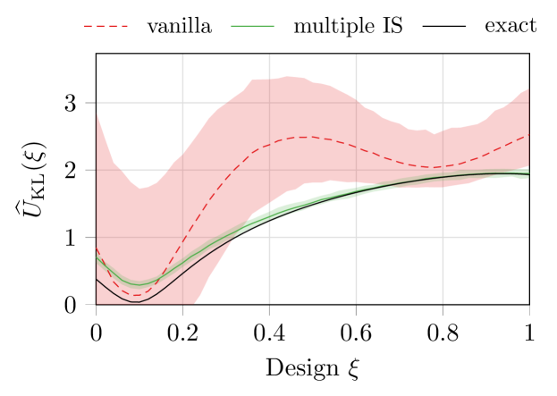
Figure 3.1: Estimated EIG as a function of a scalar design parameter $\xi$ for a linear-Gaussian model, using vanilla NMC (red) or an improved multiple importance sampling scheme (green), compared to the true EIG (black). Shaded areas represent the interval containing 95% of 2000 independent estimates of EIG at each $\xi$; red dashed and solid green lines are the means of these estimates. Figure adapted from Feng and Marzouk (2019).

3.2 Mutual information bounds via density approximations

As anticipated in the discussion following (21)–(22), one of the core computational tasks of the NMC estimators discussed in Section 3.1 is to estimate the posterior normalizing constant $p(y|\xi)$ across many different values of $y$. The vanilla NMC approach does this entirely independently for each value of $y$, as does the Laplace-based importance sampling method. (The adaptive importance sampling scheme of Feng and Marzouk (2019), on the other hand, could be said to ‘borrow’ information from other values of $y$ to create a local biasing distribution.) A rather different way of approaching this problem is to approximate the marginal density $p(y|\xi)$, or similarly, the normalized posterior density $p(\theta|y,\xi)$, directly, e.g., in some parametric family of densities.

Let us recall (21)–(23) in a more concise form:

$$\mathcal{I}(Y;\Theta|\xi) =\mathbb{E}_{Y,\Theta|\xi}\left[\log\frac{p(Y|\Theta,\xi)}{p(Y|\xi)}\right]$$ (60)

$$=\mathbb{E}_{Y,\Theta|\xi}\left[\log\frac{p(\Theta|Y,\xi)}{p(\Theta)}\right].$$ (61)

In either (60) or (61), one could in principle seek to approximate the density in the numerator, the density in the denominator, or both. Suppose that we replace $p(y|\xi)$ in (60) with some approximating probability density function $q^{\text{mar}}(y|\xi)$ (where the superscript stands for ‘marginal’). Then, as noted in Barber and Agakov (2003), Poole et al. (2019), and Foster et al. (2019),

$$\mathcal{I}(Y;\Theta|\xi) =\mathbb{E}_{Y,\Theta|\xi}\left[\log\frac{p(Y|\Theta,\xi)\,q^{\text{mar}}(Y|\xi)}{q^{\text{mar}}(Y|\xi)\,p(Y|\xi)}\right]$$

$$=\mathbb{E}_{Y,\Theta|\xi}\left[\log\frac{p(Y|\Theta,\xi)}{q^{\text{mar}}(Y|\xi)}\right]-D_{\text{KL}}(p_{Y|\xi}||q^{\text{mar}}_{Y|\xi})$$

$$\leq\mathbb{E}_{Y,\Theta|\xi}\left[\log\frac{p(Y|\Theta,\xi)}{q^{\text{mar}}(Y|\xi)}\right]=\mathbb{E}_{\Theta}\left[D_{\text{KL}}(p_{Y|\Theta,\xi}||q^{\text{mar}}_{Y|\xi})\right],$$ (62)

where the inequality follows from the non-negativity of the KL divergence. Hence, for any approximation $q^{\text{mar}}(y|\xi)$ of the marginal density of $Y|\xi$, (62) is an upper bound on the mutual information (EIG).

Similarly, if we replace $p(\theta|y,\xi)$ in (61) with some approximating probability density function $q^{\text{pos}}(\theta|y,\xi)$ (where the superscript denotes ‘posterior’), we obtain

$$\mathcal{I}(Y;\Theta|\xi) =\mathbb{E}_{Y,\Theta|\xi}\left[\log\frac{q^{\text{pos}}(\Theta|Y,\xi)\,p(\Theta|Y,\xi)}{p(\Theta)\,q^{\text{pos}}(\Theta|Y,\xi)}\right]$$

$$=\mathbb{E}_{Y,\Theta|\xi}\left[\log\frac{q^{\text{pos}}(\Theta|Y,\xi)}{p(\Theta)}\right]+\mathbb{E}_{Y|\xi}\left[D_{\text{KL}}(p_{\Theta|Y,\xi}||q^{\text{pos}}_{\Theta|Y,\xi})\right]$$

$$\geq\mathbb{E}_{Y,\Theta|\xi}\left[\log\frac{q^{\text{pos}}(\Theta|Y,\xi)}{p(\Theta)}\right]=\mathbb{E}_{Y,\Theta|\xi}[\log q^{\text{pos}}(\Theta|Y,\xi)]+H(\Theta).$$ (63)

Hence, for any approximation $q^{\text{pos}}(\theta|y,\xi)$ of the posterior density, (63) is a lower bound on the mutual information (EIG). This bound is sometime called the Barber–Agakov bound, after Barber and Agakov (2003). Note that all expectations above, and specifically in (62) and (63), are with respect to the true distribution $p_{Y,\Theta|\xi}$.

Evaluating the upper bound (62) requires the ability to evaluate the likelihood function, and thus it does not apply to the implicit model setting where the likelihood is intractable. Evaluating the lower bound, on the other hand, only requires access to the prior density (or the differential entropy of the prior) and the ability to find a tractable approximation $q^{\text{pos}}(\theta|y,\xi)$.

Foster et al. (2019) were the first to suggest using these mutual information bounds in OED, and in practice selected the approximations $q$ from simple parametric families of densities (e.g., Gaussian, uniform) that were tailored to the design problem at hand. Once such a family $\mathcal{Q}$ is specified, the best member of the family—i.e., the density yielding the closest approximation of the EIG—can be found by tightening the bound. Specifically, for the marginal approximation, we seek (for any given design $\xi$)

$$q^{\text{mar},\ast}\in\operatornamewithlimits{argmax}_{q\in\mathcal{Q}}\mathbb{E}_{Y|\xi}\left[\log q(Y|\xi)\right],$$ (64)

which minimizes the upper bound (62), while for the posterior approximation we seek

$$q^{\text{pos},\ast}\in\operatornamewithlimits{argmax}_{q\in\mathcal{Q}}\mathbb{E}_{Y,\Theta|\xi}\left[\log q(\Theta|Y,\xi)\right],$$ (65)

which maximizes the lower bound (63). In practice, the expectations in (64) or (65) are approximated using samples from the model; for example, (64) becomes

$$\hat{q}^{\text{mar}}\in\operatornamewithlimits{argmax}_{q\in\mathcal{Q}}\sum_{i=1}^{M}\log q(y^{(i)}|\xi),\quad y^{(i)}\sim p(y|\xi),$$ (66)

and analogously for (65). Inspecting (66), it is apparent that identifying a member of the variational family in this way is none other than maximum likelihood estimation of either the marginal density $p(y|\xi)$ or conditional density $p(\theta|y,\xi)$.

With this link in mind, we can immediately generalize the machinery used to construct good density approximations. One powerful approach for estimating both joint and conditional densities rests on transportation of measure (Villani 2009, Marzouk et al. 2016, Spantini et al. 2018). Given some generic target distribution $\pi$ on $\mathbb{R}^{d}$, the idea behind transport methods is to find an invertible transformation $S:\mathbb{R}^{d}\to\mathbb{R}^{d}$ that pushes forward $\pi$ to a simple reference distribution $\rho$ on $\mathbb{R}^{d}$ whose density can be easily evaluated. Abusing notation (by not distinguishing measures from densities), we can write this as $S_{\sharp}\pi=\rho$, which means that $\rho(A)=\pi\left(S^{-1}(A)\right)$ for any $\rho$-measurable set $A$. Crucially, for any diffeomorphism $\tilde{S}$ on $\mathbb{R}^{d}$, the distribution $\tilde{S}^{\sharp}\rho\coloneqq\tilde{S}^{-1}_{\sharp}\rho$, called the pullback of $\rho$ under $\tilde{S}$, has a closed-form expression for its density:

$$\tilde{S}^{\sharp}\rho=(\rho\circ\tilde{S})\,\det\nabla\tilde{S},$$ (67)

which is guaranteed to be positive and to integrate to one. Density estimation can thus be recast as the problem of finding a map $\tilde{S}$ in some suitable class such that $\tilde{S}^{\sharp}\rho$ is ‘close’ to $\pi$ (Wang and Marzouk 2022).

In practice, these models can be quite expressive. Any measure absolutely continuous with respect to the Lebesgue measure on $\mathbb{R}^{d}$ can be represented as the pullback, under some map, of a Gaussian $\rho$ on $\mathbb{R}^{d}$; in fact, for any pair of equivalent continuous measures $(\rho,\pi)$, there exist infinitely many transport maps $S$ that achieve $S^{\sharp}\rho=\pi$. Normalizing flows (Kobyzev et al. 2020, Papamakarios et al. 2021) are a special case of this formulation, i.e., a particular class of transport map parameterizations that guarantee invertibility, differentiability, and easy evaluation of the Jacobian determinant $\det\nabla S$. But many other representations are useful. Monotone triangular maps (Bogachev et al. 2005), for instance, can represent arbitrary absolutely continuous distributions and be parameterized in a way that endows the maximum likelihood estimation problems (64)–(65) with optimization guarantees; see Baptista et al. (2023) for details. Continuous optimal transport maps can also be estimated by first solving a discrete optimal transport problem (i.e., between empirical measures) and smoothing the result (Manole et al. 2021, Pooladian and Niles-Weed 2021) or by parameterizing a differentiable convex potential (Huang et al. 2020).

In the context of OED, it is useful to employ block-triangular maps (Baptista et al. 2024b) (a class which includes strictly triangular maps but infinitely many other choices), as they naturally capture conditional densities. Consider the following block arrangement for a map $S:\mathbb{R}^{n+p}\to\mathbb{R}^{n+p}$:

$$S(y,\theta)=\begin{bmatrix}[l]S^{Y}(y)\\ S^{\Theta}(y,\theta)\end{bmatrix},$$ (68)

where $S^{Y}:\mathbb{R}^{n}\to\mathbb{R}^{n}$ and $S^{\Theta}:\mathbb{R}^{n+p}\to\mathbb{R}^{p}$. Let the reference distribution $\rho$ on $\mathbb{R}^{n+p}$ factor as $\rho=\rho_{n}\otimes\rho_{p}$, where the subscripts denote the dimension of the factors. (The standard Gaussian distribution on $\mathbb{R}^{n+p}$ naturally factorizes in this way, but any distribution with appropriate block-independence would suffice.) Then, as shown in Baptista et al. (2024b) and Marzouk et al. (2016), if $S_{\sharp}p_{Y,\Theta}=\rho$, then $S^{Y}_{\sharp}p_{Y}=\rho_{n}$ and $\bigl{(}\theta\mapsto S^{\Theta}(y,\theta)\bigr{)}_{\sharp}p_{\Theta|Y=y}=\rho_{p}$ for any $y\in\operatorname{supp}p_{Y}$. Thus the two component functions of the map capture the evidence ($Y$-marginal) and the posterior, respectively. Note also that (68) can easily be extended to depend on the design, that is,

$$S(y,\theta;\xi)=\begin{bmatrix}[l]S^{Y}(\xi,y)\\ S^{\Theta}(\xi,y,\theta)\end{bmatrix}.$$ (69)

Suppose now that we obtain a maximum likelihood estimate $\widehat{S}$ of a map of the form (69), given samples from $p(y,\theta|\xi)$ and some tractable class of candidate block-triangular maps $\mathcal{S}$, for instance as described in Baptista et al. (2023):

$$\widehat{S}(\,\cdot\,\,;\xi)\in\arg\max_{S\in\mathcal{S}}\sum_{i=1}^{M}\log S^{\sharp}\rho(y^{(i)},\theta^{(i)}).$$ (70)

The map $\widehat{S}$ yields a plug-in estimate of the desired densities, via its two component functions:

$$\hat{q}^{\text{mar}}(y|\xi) =\rho_{n}\bigl{(}\widehat{S}^{Y}(\xi,y)\bigr{)}\det\nabla_{y}\widehat{S}^{Y}(\xi,y),$$

$$\hat{q}^{\text{pos}}(\theta|y,\xi) =\rho_{p}\bigl{(}\widehat{S}^{\Theta}(\xi,y,\theta)\bigr{)}\det\nabla_{\theta}\widehat{S}^{\Theta}(\xi,y,\theta).$$

(For a statistical convergence analysis of transport-based density estimators, in a general nonparametric setting, see Wang and Marzouk 2022.) In fact, since the reference $\rho$ is a product distribution, (70) splits into two separate optimization problems such that the component functions $S^{Y}$ and $S^{\Theta}$ can be estimated separately, and hence only the component needed for the desired variational bound needs to be learned. The resulting density estimates $\hat{q}^{\text{mar}}$ or $\hat{q}^{\text{pos}}$ can then be substituted into (62) or (63), respectively. The transport approach effectively defines the approximating class of densities $\mathcal{Q}$ in (64) or (65) as the set of all densities that can be expressed as $S^{\sharp}\rho$ for $S\in\mathcal{S}$.

Several recent instantiations of this transport approach in OED have parameterized the maps as normalizing flows; see Kennamer et al. (2023), Orozco et al. (2024), and Dong et al. (2024). In particular, the lower component function $S^{\Theta}$ can be represented as a conditional normalizing flow, which is essentially a structured invertible function of $\theta$ that is parameterized by $y$. Another canonical choice of $S^{\Theta}$ is a conditional Brenier map (Carlier et al. 2016), which can be understood as a family of $L^{2}$-optimal transport maps from $p_{\Theta|Y=y}$ to $\rho_{p}$, parameterized by $y$. The essential requirements are to respect the overall block structure of (68) in an invertible, differentiable map that pushes forward $p_{Y,\Theta}$ to a block-independent reference distribution.

Figure 3.2, adapted from Li et al. (2024a), shows an application of transport-based density estimators to the nonlinear Mössbauer spectroscopy example described in Feng and Marzouk (2019, Section 4.2), for a fixed design $\xi$. The orange violin plots and circles show repeated independent estimates of the upper bound (62), while the blue violin plots and circles illustrate repeated independent estimates of the lower bound (63). These estimates are produced by learning the appropriate transport map component, $S^{Y}$ or $S^{\Theta}$, via the adaptive semi-parametric procedure described in Baptista et al. (2023), which naturally enlarges the family of maps being considered as the sample size available for estimation increases. Here the maps $S$ are strictly triangular, and hence approximations of the Knothe–Rosenblatt rearrangement; see Rosenblatt (1952), Knothe (1957) and Santambrogio (2015, Section 2.3). The horizontal axis shows the total number of independent samples drawn from the model, comprising two batches: one to estimate the map and a separate batch to estimate the outer expectations $\mathbb{E}_{Y,\Theta|\xi}$ in (62) and (63). (Asymptotically optimal allocations of this sample budget are discussed in Li et al. (2024a).) The upper and lower bounds ‘sandwich’ the true EIG as the sample size increases.

It is useful to understand the source and nature of the randomness in these results. Each estimate of a transport map yields a density estimate $\hat{q}$, and plugging any such estimate into (62) and (63) yields a guaranteed upper or lower bound, as appropriate. Approximating the expectations in (62) and (63) with samples, however, yields an unbiased estimate of the bound. There is no guarantee that each realization of the estimator will be above or below the true EIG, though the figure suggests that no realizations cross this threshold at the sample sizes considered here. Overall, however, fluctuation in the estimates reflects randomness in both $\hat{q}$ and in the Monte Carlo approximation of the outer expectation. The red dashed line in Figure 3.2 is an NMC estimate of the EIG obtained with $1.58\times 10^{6}$ samples, which is two to four orders of magnitude greater than the number of samples used in the variational estimators. The NMC estimate appears to be positively biased, even at this large sample size.

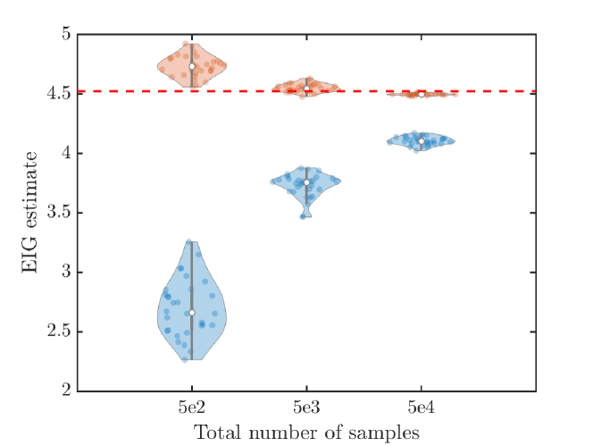
Figure 3.2: Variational upper (orange) and lower (blue) bounds on the EIG in a nonlinear design problem, compared to a biased estimate obtained via NMC (dashed red line). See the discussion in Section 3.2. Figure adapted from Li et al. (2024a).

As noted earlier, estimating the posterior density to construct a lower bound for EIG is well suited to implicit models, since (63) does not require the ability to evaluate $p(y|\theta,\xi)$. But the flexibility of using such density estimates also applies to other information-based design criteria discussed in Section 2.2.2. For instance, the expected marginal information gain objective in (28) can be bounded from below by estimating $p(\theta_{1}|y,\xi)$, i.e., by replacing this marginal posterior density with some $q(\theta_{1}|y,\xi)$. Baptista et al. (2024a) uses this approach to assess the information value of different observables in a phase-field model (a nonlinear PDE), where high-dimensional random initial conditions take the role of the ‘nuisance parameters’ $\Theta_{2}$. If the prior marginal density $p(\theta_{1})$ is not available in closed form, it can also be estimated from samples, with the caveat that if $p(\theta_{1}|y,\xi)$ and $p(\theta_{1})$ are both replaced with approximations, the resulting EIG approximation will be neither an upper nor a lower bound for the true marginal EIG in general (Foster et al. 2019).

In the case of goal-oriented OED (31)–(32), the need for learning both the numerator and denominator in the associated density ratios is more acute: for a generic $\Psi$, none of the densities in (31) or (32) may be readily available. But as long as we can simulate from $p(z,y|\xi)$—which can be done by drawing $\theta^{(i)}\sim p(\theta)$, drawing $y^{(i)}\sim p(y|\theta^{(i)},\xi)$, and evaluating $z^{(i)}=\Psi(\theta^{(i)})$—the density estimation techniques discussed above will apply. If we choose to use transport in this setting, then two block-triangular maps will be relevant:

$$S_{1}(y,z;\xi)=\begin{bmatrix}[l]S_{1}^{Y}(\xi,y)\\[6.0pt] S_{1}^{Z}(\xi,y,z)\end{bmatrix}\quad\text{and}\quad S_{2}(z,y;\xi)=\begin{bmatrix}[l]S_{2}^{Z}(\xi,z)\\[6.0pt] S_{2}^{Y}(\xi,z,y)\end{bmatrix}.$$ (71)

Approximating the densities in (31) would use the lower component of $S_{1}$ and the upper component of $S_{2}$; conversely, approximating the densities in (32) would use the upper component of $S_{1}$ and the lower component of $S_{2}$.

In closing, we note that transport approximations of the densities relevant to an EIG calculation can be built by means other than maximum likelihood estimation. For instance, Koval et al. (2024) first prescribe some density over the continuous real-valued design variables $\xi$, and then build triangular transport maps directly from unnormalized evaluations of the joint density $p(y,\theta|\xi)p(\xi)$, using a functional tensor-train format (Cui et al. 2023). This construction method does not correspond to tightening a variational bound, in contrast to maximizing the likelihood, but the error in EIG due to the map approximation can nonetheless be analyzed.

Finally we note that another use for the variational approximations discussed in this subsection—specifically, the approximation $q^{\text{pos}}(\theta|y,\xi)$—is as a biasing distribution in NMC estimation of EIG. This idea, proposed in Foster et al. (2019), fits directly into (57) by setting $q^{i,\xi}(\theta)=q^{\text{pos}}(\theta|y^{(i)},\xi)$ and recovers the consistency guarantees of NMC.

3.3 More general variational bounds for mutual information

So far, we have discussed bounds on mutual information that follow from parameterizing a density—or a transport map from which a density estimate can be derived. These bounds are variational in the sense that they can be tightened by solving an optimization problem over some class of densities or transport maps. For the bounds discussed so far, if the class of densities or transports is sufficiently rich, in principle there is a member of the class that corresponds to the true density and the bound will attain the true mutual information.

But there are many other variational bounds for mutual information, based on different approximation formats and more general classes of functions (i.e., not just densities or invertible transport maps). Such bounds are in fact an important topic in information theory, with many applications in machine learning. And several have found recent use in OED. Poole et al. (2019) provide a unifying framework for understanding many variational bounds, which inspires some of the discussion below.

To provide some context, we first recall a classical nonparametric estimator of mutual information (which is not variational). The $k$-nearest-neighbor estimator of Kraskov et al. (2004) (KSG) takes joint sample pairs $(y^{(i)},\theta^{(i)})\sim p_{Y,\Theta}$ as input, and uses the statistics of nearest-neighbor distances in both the joint space and in the marginal directions to construct an estimator. Its construction is related to $k$-nearest-neighbor estimators of the Shannon entropy (Kozachenko and Leonenko 1987). The KSG estimator has been used for OED (Terejanu et al. 2012), but is known to scale poorly with dimension. Rigorous statistical analyses of this estimator, e.g., proofs of consistency for fixed $k$ and bounds on the rate of convergence of the MSE with sample size $N$, have appeared relatively recently (Gao et al. 2018). For instance, Gao et al. (2018, Corollary 2) establish an upper bound on the MSE that is, up to polylogarithmic factors, $\mathcal{O}(N^{-2/(n+p)})$, where $n$ is the dimension of $Y$ and $p$ is the dimension of $X$. They suggest that this convergence rate cannot be refined even if the densities of interest are assumed to be Hölder-smooth.

Nonparametric estimators of the entropy (rather than the mutual information) have been used to construct lower bounds for mutual information in Ao and Li (2020). Here the idea is to write $\mathcal{I}(Y;\Theta|\xi)=H(Y|\xi)-H(Y|\Theta,\xi)$ and then to seek an upper bound for the conditional entropy $H(Y|\Theta,\xi)$. The authors develop an upper bound that requires only (unconditional) entropy estimation, performed via a $k$-nearest-neighbors approach (Kozachenko and Leonenko 1987).

3.3.1 Variational lower bounds and approximate density ratios

Now we turn our discussion back to variational bounds, parameterized by learnable functions. Dropping our earlier requirement that the function be a properly normalized density or a smooth invertible transport map, Poole et al. (2019) develop the following bound, which holds for any function $f:\mathbb{R}^{p}\times\mathbb{R}^{n}\to\mathbb{R}$ and any positive function $a:\mathbb{R}^{n}\to\mathbb{R}_{>0}$:

$$\mathcal{I}(Y;\Theta) \geq\mathbb{E}_{\Theta,Y}\left[f(\Theta,Y)\right]-\mathbb{E}_{Y}\left[\frac{\mathbb{E}_{\Theta}\left[e^{f(\Theta,Y)}\right]}{a(Y)}+\log a(Y)-1\right]$$

$$\eqqcolon\mathcal{L}^{\text{TUBA}}(f,a)\,.$$ (72)

Here ‘TUBA’ denotes ‘tractable unnormalized Barber–Agakov (BA),’ for reasons we will explain shortly. The function $f$ is known as the ‘critic.’ This bound is tightened by maximizing simultaneously over $f$ and $a$. Since the mutual information will generally depend on the design $\xi$, the critic and the function $a$ can both depend on the design as well, but here we have temporarily dropped dependence on $\xi$ to lighten notation. We can link this bound to the BA bound in (63), which uses variational approximation over a class of normalized densities, by writing

$$q(\theta|y)=\frac{p(\theta)}{Z(y)}e^{f(\theta,y)}$$ (73)

and

$$Z(y)=\mathbb{E}_{\Theta}[\exp f(\Theta,y)].$$ (74)

Hence $f$ parameterizes an approximation ${q(\theta|y)}/{p(\theta)}$ of the true posterior-to-prior density ratio ${p(\theta|y)}/{p(\theta)}$, and $Z$ is the $y$-dependent normalizing constant. The bound $\mathcal{L}^{\text{TUBA}}(f,a)$ is then tight when

$$f(\theta,y)=\log p(y|\theta)+c(y)\quad\text{and}\quad a(y)=Z(y),$$

where $c$ is any function of $y$. One specific case is when $c=0$, and hence $f(\theta,y)=\log p(y|\theta)$ and $a(y)=p(y)$.

Poole et al. (2019) point out that the lower bound for mutual information introduced earlier by Nguyen et al. (2010), often called the NWJ bound, is a special case of (72) that follows from setting $a=e$:

$$\mathcal{I}(Y;\Theta) \geq\mathbb{E}_{\Theta,Y}\left[f(\Theta,Y)\right]-\frac{1}{e}\,\mathbb{E}_{Y}\left[Z(Y)\right]\eqqcolon\mathcal{L}^{\text{NWJ}}(f).$$ (75)

In this case, the unique optimal critic is

$$f^{\ast}(\theta,y)=1+\log\frac{p(\theta|y)}{p(\theta)}.$$

Unbiased estimates of these lower bounds, for any $f$ and $a$, can be constructed by simple Monte Carlo estimation of the expectations therein. Similarly, one can produce unbiased estimates of the gradient of each bound with respect to $f$ and $a$ (or some parameterization thereof). The modern approach is to parameterize $f$ and $a$ with deep neural networks, and to maximize over the network parameters, with the hope that the resulting class of functions is rich enough to yield a good approximation of the optimal critic. The statistical properties of these nonlinear M-estimators are not yet fully understood, though there are some recent results. For instance, Sreekumar and Goldfeld (2022) develop non-asymptotic error bounds for neural estimators of statistical divergences, using shallow neural network parameterizations of $f$ (i.e., with a single hidden layer) and under strong smoothness assumptions, capturing the impact of sample size and neural network size. Statistical convergence results have also been developed for the NWJ estimator in the more classical setting where the critic is constrained to lie in a reproducing kernel Hilbert space and parameterized with kernels (Nguyen et al. 2010).

A more general observation is that while these variational bounds can in principle become tight, their estimators exhibit high variance—especially when the true value of the mutual information is large; see McAllester and Stratos (2020) for a discussion.

For completeness, we should note that the classical Donsker–Varadhan bound (Donsker and Varadhan 1983), a variational lower bound on KL divergence, can be adapted to mutual information to yield

$$\mathcal{I}(Y;\Theta) \geq\mathbb{E}_{\Theta,Y}\left[f(\Theta,Y)\right]-\log\mathbb{E}_{Y}\left[Z(Y)\right]\eqqcolon\mathcal{L}^{\text{DV}}(f).$$ (76)

When the critic $f$ is parameterized by a neural network, this is the ‘mutual information neural estimation’ (MINE) approach of Belghazi et al. (2018). The challenge in using this bound is that the second term on the right yields a nested expectation, following the definition of $Z$ in (74). Hence, in practice, when estimating the bound with Monte Carlo as in Belghazi et al. (2018), we revert to the NMC setting of Section 3.1, where estimates are biased at finite inner loop sample sizes. Then, as emphasized in Poole et al. (2019), we will obtain (to leading order) a positively biased estimator of a lower bound. The mean of this estimator is neither an upper nor a lower bound on the desired $\mathcal{I}(Y;\Theta)$.

3.3.2 Multi-sample lower bounds

A different class of lower bounds are called ‘multi-sample’ in that they involve not only an expectation over the joint distribution of $\Theta,Y\sim p_{\Theta,Y}$ but simultaneously another expectation over $\Theta_{2:M}\sim\prod_{j=2}^{M}r_{\Theta}$, where $r_{\Theta}$ could be different from the marginal $p_{\Theta}$.

The simplest among these is the so-called ‘prior contrastive estimator’ (PCE) proposed in Foster et al. (2020):

$$\mathcal{I}(Y;\Theta) \geq\mathbb{E}_{Y_{1}|\Theta_{1}}\mathbb{E}_{\Theta_{1}}\mathbb{E}_{\Theta_{2:M}}\left[\log\frac{p(Y_{1}|\Theta_{1})}{\frac{1}{M}\sum_{j=1}^{M}p(Y_{1}|\Theta_{j})}\right]\eqqcolon\mathcal{L}^{\text{PCE}}(M),$$ (77)

where the expectation is over $\Theta_{1},Y_{1}\sim p_{\Theta,Y}$ and $\Theta_{2:M}\stackrel{{\scriptstyle\text{iid}}}{{\sim}}p_{\Theta}$. Keep in mind that to estimate the right-hand side of (77), one must draw many independent and identically distributed (i.i.d.) realizations of $(Y_{1},\Theta_{1},\Theta_{2:M})$. Suppose that we draw $N$ such (outer-loop) realizations, with sample index $i$. The result is very much like the NMC estimator (53), with one crucial modification: each outer loop sample of the parameters, $\Theta_{1}^{(i)}$, is used once more, within the inner-loop estimate of the evidence for the corresponding $Y_{1}^{(i)}$. Doing so guarantees that $\mathcal{L}^{\text{PCE}}(M)$ is a lower bound of the mutual information for any $M>1$; moreover, like NMC, the bound becomes tight as $M\to\infty$ (Foster et al. 2020, Theorem 1). Intuitively, recycling the outer-loop parameter sample makes the denominator of (77) over-estimate the evidence and hence under-estimate the mutual information. The samples $\Theta_{2:M}^{(i)}$ are called contrastive samples, in that, unlike the original sample $\Theta_{1}^{(i)}$, they are not responsible for $Y_{1}^{(i)}$.

Just as the variance and bias of the NMC estimators in Section 3.1 were improved by importance sampling, a $y$-dependent, properly normalized, biasing distribution $q(\theta|y)$ can be used within a contrastive estimator as well. (The biasing distribution will generally depend on $\xi$ too, but recall that we are not explicitly writing dependence on $\xi$ in this section, to keep notation simple.) This leads to the idea of an ‘adaptive contrastive estimator’ (ACE) proposed by Foster et al. (2020),

$$\mathcal{I}(Y;\Theta) \geq\mathbb{E}_{Y_{1},\Theta_{1}}\mathbb{E}_{\Theta_{2:M}}\left[\log\frac{p(Y_{1}|\Theta_{1})}{\frac{1}{M}\sum_{j=1}^{M}\frac{p(Y_{1}|\Theta_{j})p(\Theta_{j})}{q(\Theta|Y_{1})}}\right]\eqqcolon\mathcal{L}^{\text{ACE}}(M,q),$$ (78)

where now the expectation is over $\Theta_{1},Y_{1}\sim p_{\Theta,Y}$ and $\Theta_{2:M}\stackrel{{\scriptstyle\text{iid}}}{{\sim}}q_{\Theta|Y_{1}}$. The optimal biasing distribution in this case is $q(\theta|y)=p(\theta|y)$, which leads to zero-variance estimates of the evidence $p(Y_{1})$. Seeking this $q$ is exactly the idea described at the end of Section 3.2—combining a variational approximation of the posterior density with nested Monte Carlo—with only the addition of a contrastive recycling of the outer-loop $\Theta_{1}$. With the optimal choice of $q$, this bound is tight for any finite $M$; otherwise, for sub-optimal $q$, it becomes tight as $M\to\infty$.

Both (77) and (78) require the ability to evaluate the likelihood, and thus in contrast with the variational bounds (63), (72), and (75), they are not suited to implicit models. A further modification can make (77) likelihood-free. It introduces a critic function $f$ as follows:

$$\mathcal{I}(Y;\Theta) \geq\mathbb{E}_{Y_{1},\Theta_{1}}\mathbb{E}_{\Theta_{2:M}}\left[\log\frac{\exp f(\Theta_{1},Y_{1})}{\frac{1}{M}\sum_{j=1}^{M}\exp f(\Theta_{j},Y_{1})}\right]\eqqcolon\mathcal{L}^{\text{NCE}}(M,f),$$ (79)

where the expectation is again over $\Theta_{1},Y_{1}\sim p_{\Theta,Y}$ and $\Theta_{2:M}\stackrel{{\scriptstyle\text{iid}}}{{\sim}}p_{\Theta}$. This is essentially the ‘information noise-contrastive estimation’ (InfoNCE) approach proposed in van den Oord et al. (2018). $\mathcal{L}^{\text{NCE}}(M,f)$ is a lower bound of the mutual information for all $f$ and $M$ (Poole et al. 2019). An amalgam of (78) and (79), incorporating both a biasing distribution $q$ and a critic $f$, is called ‘likelihood-free ACE’ in Foster et al. (2020). We note that both $\mathcal{L}^{\text{PCE}}(M)$ and $\mathcal{L}^{\text{NCE}}(M,f)$ are bounded above by $\log(M)$—no matter how the critic is chosen in the latter. Hence if $\mathcal{I}(Y;\Theta)>\log(M)$, these contrastive bounds cannot become tight; caution is therefore needed when the mutual information is high or the contrastive sample size $M$ is small. Note also that the $\log(M)$ limit does not apply to (78) and to other variants that use importance sampling, because in principle there exists a biasing distribution that yields a zero-variance estimate of the evidence, and in such a case even $M=1$ is sufficient.

An alternative way of estimating the PCE and InfoNCE bounds given only a single set of i.i.d. sample pairs $(Y_{i},\Theta_{i})_{i=1}^{M}\sim p_{Y,\Theta}$ is to rotate the role of the ‘data-generating sample’ and the ‘contrastive samples’ through the set. We can take the $i$th pair as the ‘data-generating sample’ and use the remaining $M-1$ samples as ‘contrastive samples’ to obtain

$$\log\frac{\exp f(\Theta_{i},Y_{i})}{\frac{1}{M}\sum_{j=1}^{M}\exp f(\Theta_{j},Y_{i})}.$$

Repeating this for $i=1,\ldots,M$ so that each pair has the opportunity to be the ‘data-generating sample,’ and then taking the average, we obtain the estimator,

$$\frac{1}{M}\sum_{i=1}^{M}\log\frac{\exp f(\Theta_{i},Y_{i})}{\frac{1}{M}\sum_{j=1}^{M}\exp f(\Theta_{j},Y_{i})}.$$ (80)

As shown in Poole et al. (2019), the expectation of this estimator is a lower bound of the true mutual information, for any critic $f$:

$$\mathcal{I}(Y;\Theta) \geq\mathbb{E}_{(Y_{i},\Theta_{i})_{i=1}^{M}}\left[\frac{1}{M}\sum_{i=1}^{M}\log\frac{\exp f(\Theta_{i},Y_{i})}{\frac{1}{M}\sum_{j=1}^{M}\exp f(\Theta_{j},Y_{i})}\right].$$ (81)

The expectation is also bounded above by $\log M$, in the same way as (77) and (79) above. Inequality (81) is in fact the form of InfoNCE bound originally proposed in van den Oord et al. (2018). It is in essence the same as (79) but using correlated, rather than independent, terms to estimate the expectation of

$$\log\Bigl{(}\exp f(\Theta_{1},Y_{1})\Big{/}\frac{1}{M}\sum_{j=1}^{M}\exp f(\Theta_{j},Y_{1})\Bigr{)}.$$

If the conditional density $p(y|\theta)$ is tractable, then we can replace $f$ with an optimal critic, $f(\theta,y)=\log p(y|\theta)$, such that (81) becomes

$$\mathcal{I}(Y;\Theta) \geq\mathbb{E}_{(Y_{i},\Theta_{i})_{i=1}^{M}}\left[\frac{1}{M}\sum_{i=1}^{M}\log\frac{p(Y_{i}|\Theta_{i})}{\frac{1}{M}\sum_{j=1}^{M}p(Y_{i}|\Theta_{j})}\right],$$ (82)

which can be understood as a ‘sample re-use’ analogue of the PCE bound (77) above. Interestingly, the corresponding estimator (i.e., (80) with the log-likelihood substituting for $f$) was used in Huan and Marzouk (2013), before it was formally understood to be a lower bound in expectation. There, the rationale was to lower the cost of nested Monte Carlo by reducing the number of expensive model evaluations from $\mathcal{O}(NM)$ to $\mathcal{O}(M)$, in a setting where evaluations of the likelihood $p(y|\theta)$ are costly for each new value of $\theta$, but cheap for new values of $y$ given a fixed $\theta$.

3.3.3 Deploying variational bounds

The relative merits of the variational bounds discussed above are very much a current subject of research, involving both empirical comparisons and some theory (Czyż et al. 2023, Song and Ermon 2020, Letizia et al. 2023). In general, the TUBA, NWJ, and DV bounds can become tight with increasingly good choices of critic, but their Monte Carlo estimates generally have much higher variance than estimates of multi-sample bounds such as PCE and InfoNCE. The latter bounds, on the other hand, are hampered by the fact they cannot become tight for arbitrarily large mutual information when using finite contrastive sample sizes. We also emphasize that new variants of these variational bounds continue to be proposed; we have attempted to cover the key constructions relevant to OED, but do not claim to be comprehensive. We refer to Song and Ermon (2020) and Czyż et al. (2023) for empirical evaluations of the mutual information estimators (and estimators of mutual information bounds) discussed here, along with many others. Important settings for these evaluations include low versus high values of mutual information, heavy versus light tails, various forms of non-Gaussianity, high dimensionality, sparse interactions, and so forth. As emphasized by Czyż et al. (2023), evaluations limited to the Gaussian setting, while convenient in that exact analytical results are available for comparison, are not fully representative.

Deploying the bounds discussed in Sections 3.2 and 3.3 requires optimization. Specifically, it is useful to have an unbiased estimate of the gradient of each bound with respect to parameters representing the critic $f$ (and possibly $a$) or the density approximation $q$, along with an unbiased estimate of the gradient of the bound with respect to the design $\xi$, for any given critic or density approximation. Explicit forms of these gradient estimates, for several bounds above, are detailed in Kleinegesse and Gutmann (2021). Given these gradients, one can simultaneously maximize the bound with respect to both the variational parameters and the design, e.g., via stochastic gradient ascent. We will return to this idea in Section 4.3.

3.4 Low-dimensional structure

So far, we have discussed a variety of methods that, essentially, approximate the densities or density ratios appearing in expressions for the mutual information (expected information gain). A different and complementary class of approximation methods involve dimension reduction. Here we will discuss methods for Bayesian OED that exploit possible low dimensionality in the update from prior to posterior; such methods rest on the idea that the posterior is well-approximated by a distribution that departs from the prior only on a subspace of dimension $r\ll p$. At the same time, we will consider dimension reduction for the observation vector $y\in\mathbb{R}^{n}$; the central idea is that conditioning on $y$ could be replaced by conditioning on the projection of $y$ onto a subspace of dimension $s\ll n$.

Both of these notions of low dimensionality appear quite often in Bayesian inverse problems, where the data are related to the parameters $\theta$ by the action of a forward operator that is somehow smoothing, e.g., in that it suppresses information about finer scales (Cui et al. 2014). Low dimensionality more generally results from limited informativeness of the data in certain directions of $\bm{\Theta}$ and/or redundancy among the components of $y$. There is additional potential for dimension reduction in goal-oriented problems, as in Bayesian $\text{D}_{\text{A}}$-optimality and (31)–(32), where the experimenter wishes to learn about a specific quantity of interest $Z=\Psi(\Theta)$. Identifying and exploiting this low dimensionality can lead to much more computationally efficient approximations of the mutual information, as we shall discuss below.

3.4.1 Linear models

We first consider dimension reduction, of both parameters and data, in the context of finite-dimensional Bayesian linear-Gaussian models. We begin with design for parameter inference and then consider goal-oriented design.

Optimal low-rank approximations for parameter inference.

Recall the setup of the Bayesian linear-Gaussian model from the start of Section 2.1.2. The mutual information between parameters and observations in this setting can already be written in closed form as a ratio of log-determinants, as in (25) and (26). It is nonetheless useful to express this quantity in a way that reveals the structure and intrinsic dimensionality of the linear-Gaussian model.

The central objects in such a construction are generalized eigenvalue problems involving combinations of the prior covariance matrix $\Gamma_{\Theta}$; the noise covariance $\Gamma_{Y|\Theta}$; the posterior covariance $\Gamma_{\Theta|Y}$ (8); the negative Hessian of the log-likelihood, $H\coloneqq G^{\top}\Gamma_{Y|\Theta}^{-1}G$; and the marginal covariance of the data, $\Gamma_{Y}=G\Gamma_{\Theta}G^{\top}+\Gamma_{Y|\Theta}$. Several different generalized eigenvalue problems involving these matrices can be written, all closely related via simple transformations. Perhaps the most direct is the symmetric definite generalized eigenproblem

$$Hw_{j}=\lambda_{j}\Gamma_{\Theta}^{-1}w_{j}\,,$$ (83)

where, since $H\succeq 0$ and $\Gamma^{-1}_{\Theta}\succ 0$, we have $\lambda_{j}\geq 0$. This eigenproblem can be understood as balancing informativeness of the likelihood with informativeness of the prior, via the Rayleigh ratio $w^{\top}Hw/w^{\top}\Gamma_{\Theta}^{-1}w$: an eigendirection $w_{j}\in\mathbb{R}^{p}$ associated with $\lambda_{j}>1$ is more constrained by the likelihood than by the prior, and thus more important to the update from prior to posterior. See Spantini et al. (2015) for thorough interpretations and demonstrations of this eigenstructure. Closely related to (83) are two other $p\times p$ parameter-space matrix pencils: $(\Gamma_{\Theta}-\Gamma_{\Theta|Y},\Gamma_{\Theta|Y})$ and $(\Gamma_{\Theta},\Gamma_{\Theta|Y})$. The first has eigenvalue-eigenvector pairs $(\lambda_{j},v_{j})$, where $v_{j}=\Gamma_{\Theta}^{-1}w_{j}$, and the second has eigenvalue-eigenvector pairs $(1+\lambda_{j},v_{j})$. See Jagalur-Mohan and Marzouk (2021, Proposition 10) for a proof of this equivalence. The leading eigendirections $v_{j}$ (ordered from largest to smallest $\lambda_{j}$) are the directions along which the ratio of posterior to prior variance is minimized; see Spantini et al. (2015, Section 3.1).

In the linear-Gaussian setting, there is a duality between spectral structure in the parameter space and in the data space. Consider the $n\times n$ data-space matrix pencils $(\Gamma_{Y}-\Gamma_{Y|\Theta},\Gamma_{Y|\Theta})$ and $(\Gamma_{Y},\Gamma_{Y|\Theta})$. Jagalur-Mohan and Marzouk (2021, Proposition 10) show that $(\Gamma_{Y}-\Gamma_{Y|\Theta},\Gamma_{Y|\Theta})$ and $(\Gamma_{\Theta}-\Gamma_{\Theta|Y},\Gamma_{\Theta|Y})$ have identical non-trivial generalized eigenvalues, $\lambda_{j}>0$, and that $(\Gamma_{Y},\Gamma_{Y|\Theta})$ and $(\Gamma_{\Theta},\Gamma_{\Theta|Y})$ have identical eigenvalues that are strictly greater than one, i.e., $1+\lambda_{j}>1$. The eigenvectors $u_{j}$ of the two data-space pencils are identical, with $w_{j}=\frac{1}{\alpha_{j}}\Gamma_{\Theta}G^{\top}u_{j}$ for all $j$ with $\lambda_{j}>0$, where $\alpha_{j}$ is a scaling parameter that can be set to $\alpha_{j}=\sqrt{\lambda_{j}}$ to obtain $\langle U_{i},U_{j}\rangle_{\Gamma_{Y|\Theta}}=\delta_{ij}$, given $\langle W_{i},W_{j}\rangle_{\Gamma_{\Theta}^{-1}}=\delta_{ij}$.

A convenient way of simultaneously capturing spectral structure in the parameter space and the data space is through the ‘whitened’ forward operator $\Gamma_{Y|\Theta}^{-1/2}G\Gamma_{\Theta}^{1/2}$. The singular value decomposition of this matrix is

$$\Gamma_{Y|\Theta}^{-1/2}G\Gamma_{\Theta}^{1/2}=\sum_{j\geq 1}\sqrt{\lambda_{j}}a_{j}b_{j}^{\top},$$

where the left singular vectors are related to the preceding data-space eigendirections via $a_{j}=\Gamma_{Y|\Theta}^{1/2}u_{j}$ and the right singular vectors similarly are $b_{j}=\Gamma_{\Theta}^{-1/2}w_{j}$. See also Spantini et al. (2015, Remark 4). The whitened forward operator thus summarizes much of the essential structure of the linear-Gaussian Bayesian inverse problem and appears in many contexts. In the case of uncorrelated observational errors $\Gamma_{Y|\Theta}=\sigma^{2}I$, for example, the adjoint of the whitened forward operator, $\sigma^{-1}\Gamma_{\Theta}^{1/2}G^{\top}$, is the central object in column subset selection approaches to finding D-optimal designs (Eswar et al. 2024). We will comment further on these methods in Section 4.

Spantini et al. (2015, Theorem 2.3) consider optimal approximations of the posterior covariance $\Gamma_{\Theta|Y}$ that take the form of low-rank updates of the prior covariance. Optimality is cast in terms of minimizing a class of loss functions $\ell(M)$ over the manifold of all symmetric positive definite (SPD) matrices $M$; this class includes the geodesic distance from $M$ to $\Gamma_{\Theta|Y}$ on SPD manifold, and the KL divergence or Hellinger distance from $\mathcal{N}(\mu,M)$ to $\mathcal{N}(\mu,\Gamma_{\Theta|Y})$, where $\mu\in\mathbb{R}^{p}$ is an arbitrary (common) mean vector. The approximations sought are of the form $\widetilde{\Gamma}^{r}_{\Theta|Y}\in\{\Gamma_{\Theta}-KK^{T}\succ 0,\ \text{rank}(K)\leq r\}$, and the optimal approximation for any $r\leq n$, simultaneously minimizing all loss functions in the class, is given by

$$KK^{\top}=\sum_{i=1}^{r}\frac{\lambda_{i}}{1+\lambda_{i}}w_{i}w_{i}^{\top};$$

hence it follows from the leading eigenpairs of the parameter-space pencil $(H,\Gamma_{\Theta}^{-1})$. The decay of the eigenvalue sequence $(\lambda_{j})_{j\geq 1}$, common to all of the matrix pencils above, captures the intrinsic dimensionality of the Bayesian model.

These optimal approximation results are related to the approximation of a more central object of interest in OED: the mutual information. Using the fact that the generalized eigenvectors $v_{j}$ simultaneously diagonalize $\Gamma_{\Theta}$ and $\Gamma_{\Theta|Y}$, or that the generalized eigenvectors $u_{j}$ simultaneously diagonalize $\Gamma_{Y}$ and $\Gamma_{Y|\Theta}$, the mutual information between parameters $\Theta$ and data $Y$ (25)–(26) can be written as

$$\mathcal{I}(Y;\Theta)=\frac{1}{2}\sum_{j}\log(1+\lambda_{j})\,.$$ (84)

This expression for mutual information has appeared in many places in recent literature, e.g., Alexanderian et al. (2016a) and Giraldi et al. (2018). We note also that $\mathcal{I}(Y;\Theta)$ can be written using the squared canonical correlation scores (Bach and Jordan 2002) between $Y$ and $\Theta$; these scores follow from generalized eigenvalue problems that are slightly different from those discussed above, but closely related. Truncating the sum in (84) after $r<\min(n,p)$ terms yields a low-rank approximation of the mutual information. From a computational perspective, since the MI is dominated by the largest generalized eigenvalues (though the $\log$ function slows this decay), problems with quickly decaying spectra and hence low intrinsic dimension are easier to approximate: one must compute only the leading eigenvalues of any of the matrix pencils described above.

Truncating (84) in this way in fact corresponds to the mutual information obtained from an optimal $r$-dimensional projection of the data $Y$, of the parameters $\Theta$, or of both simultaneously. Specifically, Giraldi et al. (2018) show that the leading eigenvectors $U_{1:r}=[u_{1}\cdots u_{r}]$ of the data-space matrix pencils define low-dimensional projections of the data that are optimal at any given dimension $r\leq n$, in the sense of maximizing $\mathcal{I}(A_{r}^{\top}Y;\Theta)$ over matrices $A\in\mathbb{R}^{n\times r}$. The resulting mutual information is

$$\mathcal{I}(U_{1:r}^{\top}Y;\Theta)=\frac{1}{2}\sum_{j=1}^{r}\log(1+\lambda_{j}).$$

Similarly, replacing $\Theta$ with the $r$-dimensional projection $V_{1:r}^{\top}\Theta$ yields

$$\mathcal{I}(Y;V_{1:r}^{\top}\Theta)=\frac{1}{2}\sum_{j=1}^{r}\log(1+\lambda_{j}).$$

Going further, one can show that the same, optimal value of mutual information is also achieved by

$$\mathcal{I}(U_{1:r}^{\top}Y;V_{1:r}^{\top}\Theta)=\frac{1}{2}\sum_{j=1}^{r}\log(1+\lambda_{j}).$$

Note that this truncated mutual information is equivalent to the mutual information that would be obtained if the forward operator $G$ in (4) were replaced by certain ‘projected’ versions. Define

$$\mathbb{P}_{\text{obs}}\coloneqq\Gamma_{Y|\Theta}U_{1:r}U_{1:r}^{\top}\quad\text{and}\quad\mathbb{P}_{\text{param}}\coloneqq\Gamma_{\Theta}V_{1:r}V_{1:r}^{\top}=W_{1:r}W_{1:r}^{\top}\Gamma_{\Theta}^{-1}.$$

Then one can show that

$$\mathbb{P}_{\text{obs}}G=G\mathbb{P}_{\text{param}}=\mathbb{P}_{\text{obs}}G\mathbb{P}_{\text{param}},$$ (85)

and that these projected forward operators achieve the mutual information

$$\frac{1}{2}\sum_{j=1}^{r}\log(1+\lambda_{j}).$$

We emphasize, however, that the equivalence of these three projected models, and more broadly the strict duality between parameter and observation reduction discussed above, is specific to the linear-Gaussian setting.

The expression (84) naturally appears in infinite-dimensional formulations of linear Bayesian inverse problems, as discussed in Section 2.3.1. Indeed, finding the leading eigenpairs of (83) is equivalent to constructing a low-rank approximation of the prior-preconditioned Hessian operator $\widetilde{H}$, as discussed in Alexanderian et al. (2016a). To see this intuitively in finite dimensions, note that $\widetilde{H}=\Gamma_{\Theta}^{1/2}H\Gamma_{\Theta}^{1/2}$, and that its (simple, not generalized) eigenvalue-eigenvector pairs are $(\lambda_{j},\Gamma_{\Theta}^{-1/2}w_{j})$, where $(\lambda_{j},w_{j})$ are the eigenpairs of $(H,\Gamma_{\Theta}^{-1})$. The algorithms proposed in Alexanderian and Saibaba (2018) (see also Ghattas and Willcox 2021) compute these low-rank approximations efficiently in a discretization-invariant manner, when the forward operator $G$ is described by partial differential equations.

Optimal low-rank approximations for goal-oriented design.

Now we turn to the goal-oriented linear setting. Our interest here lies not in learning the parameters $\Theta$ per se, but rather in informing a quantity of interest $Z=A^{\top}\Theta$, where $A\in\mathbb{R}^{p\times s}$ has full column rank $s<p$. Maximizing the mutual information $\mathcal{I}(Y;Z)$ is equivalent to maximizing the Bayesian $\text{D}_{\text{A}}$-optimality criterion mentioned in Section 2.1.2, and is a linear special case of (31)–(32). Now, however, there is further potential for dimension reduction, stemming from the interaction of $A$ with other elements of the problem. Intuitively, the update from the prior predictive distribution to posterior predictive distribution of $Z$ (and hence the mutual information) should be well captured by directions in the parameter space $\mathbb{R}^{p}$ that are simultaneously informed by the data (relative to the prior) and influential on $Z$. We can expect the latter consideration to help ‘screen out’ parameter directions that are dampened by $A^{\top}$. (Consider, as a limiting example, elements of the kernel of $A^{\top}$.)

This idea is formalized by Spantini et al. (2017). Beginning with the linear-Gaussian model $Y=G\Theta+\mathcal{E}$ (4), a Gaussian prior distribution $\Theta\sim\mathcal{N}(0,\Gamma_{\Theta})$ (zero mean for simplicity), and the specification of $Z=A^{\top}\Theta$, Spantini et al. (2017, Lemma 2.2) introduce an equivalent linear-Gaussian model that directly relates $Y$ and $Z$,

$$Y=GA_{\dagger}Z+\Delta,$$ (86)

where $A_{\dagger}\coloneqq\Gamma_{\Theta}A\Gamma_{Z}^{-1}$, $\Gamma_{Z}\coloneqq A^{\top}\Gamma_{\Theta}A$, $Z\sim\mathcal{N}(0,\Gamma_{Z})$ is the prior induced on $Z$, and

$$\Delta\sim\mathcal{N}(0,\Gamma_{\Delta})\quad\text{with}\quad\Gamma_{\Delta}\coloneqq\Gamma_{Y|\Theta}+G(\Gamma_{\Theta}-\Gamma_{\Theta}A\Gamma_{Z}^{-1}A^{\top}\Gamma_{\Theta})G^{\top}.$$

Crucially, these choices render the ‘effective noise’ $\Delta$ independent of $Z$. Now the low-rank approximation methods discussed earlier for the $Y$–$\Theta$ system can be applied directly to the $Y$–$Z$ system above.

For example, as a goal-oriented counterpart to (83), one can compute the leading eigenpairs of the matrix pencil $(A^{\top}_{\dagger}G^{\top}\Gamma_{\Delta}^{-1}GA_{\dagger},\Gamma_{Z}^{-1})$. Letting $(\tilde{\lambda}_{j})_{j\geq 1}$ denote the generalized eigenvalues of this pencil, arranged in descending order, we can then write the mutual information as $\mathcal{I}(Y;Z)=\frac{1}{2}\sum_{j}\log(1+\tilde{\lambda}_{j})$ and truncate this sum as desired to obtain a low-rank approximation; see Wu et al. (2023a) for more details and a first application of this approach in OED. As demonstrated in Spantini et al. (2017), $(\tilde{\lambda}_{j})$ can decay much more quickly than the spectrum $(\lambda_{j})$ of (83), yielding a more efficient approximation than would be obtained by first approximating the posterior covariance matrix of $\Theta$ and then applying $A$. Moreover, analogously to the discussion above, one can obtain optimal goal-oriented projections of the data using the leading eigenvectors of $(\Gamma_{Y},\Gamma_{\Delta})$. Each of these eigenproblems optimally balances all the ingredients of the goal-oriented inference problem: the structure of the forward operator, the scale and structure of the observational noise covariance and prior covariance, and the ultimate prediction goals.

In closing, we should point out that (as in Section 3.3) we have not explicitly noted dependence of the quantities above on the design $\xi$. Recall, however, that our generic linear-Gaussian model (4) can be written more explicitly as $Y|\Theta,\xi\sim\mathcal{N}(G(\xi)\Theta,\Gamma_{Y|\Theta}(\xi))$. Hence all of the eigenvalues, eigenspaces, and projectors described above may depend on $\xi$ via $G$ and $\Gamma_{Y|\Theta}$. The details of this dependence are problem-dependent, but it is of interest to understand how to exploit any smoothness or other regularity that may be present—for instance, by differentiating the eigenvalues $\lambda_{j}$ with respect to $\xi$. To our knowledge, algorithmic approaches in this vein are in their infancy.

3.4.2 Nonlinear models

Extending the low-dimensional structure discussed in Section 3.4.1 to nonlinear models is considerably more complex, and a subject of ongoing research. The tools we will highlight here originate in dimension reduction for Bayesian inverse problems and Bayesian statistical models more generally: likelihood-informed subspaces (Cui et al. 2014, Cui and Tong 2022), certified dimension reduction (Zahm et al. 2022, Li et al. 2024b), and related efforts. Our perspective is similar to that taken in the linear case: find the subspace of the parameter space where the posterior differs ‘most’ from the prior, which is equivalent to finding the subspace that is best informed by the data; and find the subspace of the data that is most informative of the parameters.

We focus here on the approximation of mutual information, highlighted in Baptista et al. (2022), which makes the intuitive notions just stated more precise. In the nonlinear case, it is generally difficult to find optimal low-dimensional projections. Instead, one can develop gradient-based upper bounds on the error induced by projecting $Y$ and $\Theta$ onto lower-dimension subspaces, i.e., find upper bounds on the difference

$$\mathcal{I}(Y;\Theta)-\mathcal{I}(U_{1:s}^{\top}Y;V_{1:r}^{\top}\Theta)$$

for some matrices $U_{1:s}\in\mathbb{R}^{n\times s}$ and $V_{1:r}\in\mathbb{R}^{p\times r}$, and then minimize these bounds over $U$ and $V$. (Note that the matrices $U$ and $V$ discussed in this section are generally different from the $U$ and $V$ found in Section 3.4.1.)

The key assumption underlying this analysis is that the joint distribution $p_{Y,\Theta}$ must satisfy a subspace logarithmic Sobolev inequality; see Baptista et al. (2022, Definition 2) or Zahm et al. (2022, Theorem 2.10). Letting $Z=(Y,\Theta)$ be a random variable taking values in $\mathbb{R}^{n+p}$, and letting $W\in\mathbb{R}^{(n+p)\times(n+p)}$ be a unitary matrix, the essence of this assumption is that any conditional distribution $p(Z_{t}|Z_{\perp}=z_{\perp})$ defined by the decomposition $W=[W_{t}\ W_{\perp}]$, with $W_{t}\in\mathbb{R}^{(n+p)\times t}$, $Z_{t}=W_{t}^{\top}Z$, and $Z_{\perp}=W_{\perp}^{\top}Z$, satisfies a logarithmic Sobolev inequality with constant $C\left(p(Z_{t}|Z_{\perp}=z_{\perp})\right)$ bounded above by some $\overline{C}<\infty$, for all $W$, $t$, and $z_{\perp}$. As shown in Zahm et al. (2022), a sufficient condition for a distribution to satisfy the subspace logarithmic Sobolev inequality is that it has convex support and that its log-density is a bounded perturbation of a strongly convex function; see Zahm et al. (2022, Examples 2.5–2.9) and Baptista et al. (2022, Examples 1–2). This allows, for example, Gaussian mixtures (and hence certain multi-modal distributions with strictly positive densities) but not distributions with exponential tails.

Now define the diagnostic matrices

$$H_{\Theta} =\iint(\nabla_{\theta}\nabla_{y}\log p_{Y|\Theta}(y|\theta))^{\top}(\nabla_{\theta}\nabla_{y}\log p_{Y|\Theta}(y|\theta))p_{Y,\Theta}(y,\theta)\,\mathrm{d}\theta\,\mathrm{d}y,$$ (87)

$$H_{Y} =\iint(\nabla_{\theta}\nabla_{y}\log p_{Y|\Theta}(y|\theta))(\nabla_{\theta}\nabla_{y}\log p_{Y|\Theta}(y|\theta))^{\top}p_{Y,\Theta}(y,\theta)\,\mathrm{d}\theta\,\mathrm{d}y,$$ (88)

where $\nabla_{\theta}\nabla_{y}\log p_{Y|\Theta}\in\mathbb{R}^{n\times p}$. We then have the following theorem, adapted from Baptista et al. (2022).

Theorem 3.1

Let $p_{Y,\Theta}$ satisfy a subspace logarithmic Sobolev inequality with constant $\overline{C}<\infty$. Then, for any unitary matrices $V=[V_{1:r}\ V_{r+1:p}]\in\mathbb{R}^{p\times p}$ and $U=[U_{1:s}\ U_{s+1:n}]\in\mathbb{R}^{n\times n}$, we have

$$\mathcal{I}(Y;\Theta)-\mathcal{I}(U_{1:s}^{\top}Y;V_{1:r}^{\top}\Theta) \leq\overline{C}^{2}\Bigl{(}\text{tr}\bigl{(}V_{r+1:p}^{\top}H_{\Theta}V_{r+1:p}\bigr{)}+\text{tr}\bigl{(}U_{s+1:n}^{\top}H_{Y}U_{s+1:n}\bigr{)}\Bigr{)}\,.$$ (89)

Crucially, the right-hand side of (89) can be minimized for any dimensions $r\leq p$ and $s\leq n$ by choosing $V_{1:r}$ to be the leading eigenvectors of $H_{\Theta}$ and $U_{1:s}$ to be the leading eigenvectors of $H_{Y}$. This choice yields the bound

$$\mathcal{I}(Y;\Theta)-\mathcal{I}(U_{1:s}^{\top}Y;V_{1:r}^{\top}\Theta) \leq\overline{C}^{2}\left(\sum_{i=r+1}^{p}\lambda_{i}(H_{\theta})+\sum_{i=s+1}^{n}\lambda_{i}(H_{Y})\right).$$ (90)

Fast decay of the eigenvalues $\lambda_{i}$ of the two diagnostic matrices thus provides more opportunity for dimension reduction, with controlled error.

Computationally, this dimension reduction approach can be viewed as a first step towards approximating a mutual information design objective: first, find low-dimensional projections of the data and parameters, $Y_{s}=U_{1:s}^{\top}Y$ and $\Theta_{r}=V_{1:r}^{\top}\Theta$, for some $r$ and $s$, by finding the dominant eigenspaces of $H_{Y}$ and $H_{\Theta}$. (Note that, unlike in the linear-Gaussian case, the spectra of these two matrices are generally different.) Then, use any of the techniques discussed in Sections 3.1–3.3 to estimate or bound $\mathcal{I}(Y_{s};\Theta_{r})$. By the data-processing inequality (or the positivity of the right-hand side of (89)) we always have $\mathcal{I}(Y_{s};\Theta_{r})\leq\mathcal{I}(Y;\Theta)$. For example, Li et al. (2024a) use the transport-based density estimators of Section 3.2 to bound the projected mutual information $\mathcal{I}(Y_{s};\Theta_{r})$. The density estimation problems to be solved are thus of reduced dimension, and involve estimating transport maps that act on lower-dimensional spaces. Alternatively, Wu et al. (2023b) apply $V_{1:r}$ for parameter dimension reduction as proposed above, but use a simpler dimension reduction scheme for the data (principal component analysis based on the marginal covariance $\mathbb{C}\text{ov}(Y)$); both reductions are a prelude to constructing a reduced-dimensional surrogate $\widetilde{G}$ for the forward operator in a Bayesian inverse problem (see Section 3.1), and then using this surrogate within a standard nested Monte Carlo estimator of the mutual information.

In Theorem 3.1, for simplicity, we restricted the matrices $U$ and $V$ to be unitary. This constraint can effectively be relaxed by preconditioning the problem. Note that with any change of variables $\overline{\Theta}=A\Theta$ and $\overline{Y}=BY$, the left-hand side of (89) does not change, but the right-hand side does—via the diagnostic matrices and the log-Sobolev constant. It is unclear how to choose an optimal change of variables, as the log-Sobolev constant is in general very hard to compute, but one heuristic suggested in Baptista et al. (2022, Section 4), for the case of a Gaussian prior and Gaussian additive noise, is to ‘whiten’ the problem so that $\Gamma_{\overline{\Theta}}$ and $\Gamma_{\overline{Y}|\overline{\Theta}}$ become identity matrices. In the case of a linear-Gaussian model, this change of variables leads the proposed method to recover the optimal subspaces of Section 3.4.1. We also note that the change of variables need not be linear; any bijective transformation will leave the mutual information terms on the left-hand side of (89) unchanged. Thus, in principle one could compose a nonlinear change of variables with linear dimension reduction to effectively achieve nonlinear dimension reduction!

Another remark is that the bounds in Theorem 3.1 are generally not tight. One can intuitively see this in the linear-Gaussian setting where, after the linear preconditioning described above, we have $\lambda_{i}=\lambda_{i}(H_{\Theta})=\lambda_{i}(H_{Y})$. Then we can compare (84), where the exact truncation error involves logarithms of trailing eigenvalues $\log(1+\lambda_{i})$, with (90), which sums the trailing eigenvalues directly. These quantities are not the same, and the difference is analyzed in Baptista et al. (2022, Section 4.3); see also Zahm et al. (2022, Section 2.3). There is reason to believe that recent dimensional improvements to log-Sobolev inequalities (Eskenazis and Shenfeld 2024) could help tighten the bounds used here.

4 Design optimization methods

Now we will discuss methods for optimizing (generally, maximizing) OED criteria over possible designs $\xi\in\Xi$. Different representations of candidate designs and choices of design criterion can yield very different classes of optimization problems. This section will therefore review a broad array of optimization approaches, ranging from algorithms for combinatorial optimization (including continuous relaxations thereof) to gradient-based algorithms for intrinsically continuous problems. Section 4.1 focuses on exact designs for linear models, as linearity lends the problem special structure; here, we discuss various discrete algorithms, as well as convex continuous relaxations that are followed by rounding. Section 4.2 discusses exact designs for more general nonlinear problems, with design criteria treated as set functions. Section 4.3 turns to designs that are parameterized by real variables (e.g., sensor positions or times, dosages), and discusses how a variety of derivative-free or gradient-based optimization approaches interact with estimators or bounds for decision-theoretic design criteria.

4.1 Optimization methods for linear design

We state a prototypical linear design problem, by recalling the linear regression model with features $f:\mathcal{X}\to\mathbb{R}^{p}$ and uncorrelated observational errors. If the design $\xi$ is supported on $n$ equally weighted points $x_{i}\in\mathcal{X}\in\mathbb{R}^{d}$, $i=1,\ldots,n$, then the Fisher information matrix of the model is given by (11); as pointed out earlier, this expression follows from (5) by setting

$$G=\left[f(x_{1})^{\top};f(x_{2})^{\top};\ldots;f(x_{n})^{\top}\right]\in\mathbb{R}^{n\times p}$$

and $\Gamma_{Y|\theta}=\sigma^{2}I_{n}$. The classical design objectives discussed in Section 2.1 can be viewed as functions of the Fisher information matrix.

We will use the index set $\mathcal{V}\coloneqq\{1,\ldots,m\}$ to represent the support of the design space. It is instructive to think of $\mathcal{V}$ as a specific instance of $\mathcal{X}$ in the setting of a discrete design domain. In the simplest setting, the task of finding an optimal exact design amounts to selecting a set $\mathcal{S}\subseteq\mathcal{V}$ of specified cardinality $n$ that maximizes the chosen objective, i.e., any of the design criteria for linear models given in Section 2.1. More complex cases can involve constraints on the overall budget and variable costs associated with each individual design instance.

Strictly speaking, the set $\mathcal{S}$ is better characterized as a multiset, where elements can be duplicated. In a conventional set, elements are typically assumed to be different from one another. The notion of a multiset is more general, and accommodates the ‘with repetition’ scenario where a given design point can be chosen multiple times. (Repeated experiments at the same design point are not necessarily redundant, since they may yield different outcomes due to statistically independent noise.) The contrasting scenario is ‘without repetition,’ where each point is selected at most once; this is applicable, for instance, in the setting of deterministic computer experiments.

4.1.1 Local search and exchange algorithms

Algorithms guided by local search and exchange heuristics are non-sequential in nature. (We discuss sequential algorithms later in Section 4.1.3.) In the non-sequential setting, we start with an initial design of the required size, and at each iteration attempt to improve the quality of the design by deleting, adding, or exchanging points as guided by certain rules. The non-sequential nature of these algorithms implies that the resulting solution sets are non-nested, meaning that optimal design set of cardinality $n$ may look quite different from the optimal set of cardinality $n-1$ or $n+1$.

In the context of exchange algorithms, the approach of Fedorov (1972) has been quite influential. Fedorov’s exchange method starts with an arbitrary initial set $\mathcal{S}_{0}$ of $n$ candidate points, and at each iteration $t$ attempts to improve the objective by exchanging one of the points,

$$\mathcal{S}_{t}\leftarrow\{j\}\cup\mathcal{S}_{t-1}\setminus\{i\},$$

where $i\in\mathcal{S}_{t-1}$ and $j\in\mathcal{V}\setminus\mathcal{S}_{t-1}$. The search at each iteration is exhaustive: the improvement resulting from every possible exchange is calculated, and the best exchange is selected. The process is continued as long as an exchange improves the design objective.

Fedorov’s original work focused exclusively on D-optimal design, although its applicability to other design criteria has also been demonstrated. While the exchange algorithm is relatively simple, it is accompanied by a sizable computational overhead due to the exhaustive search at each step. Cook and Nachtsheim (1980) proposed a modified Fedorov exchange procedure, where they consider each design point in turn, perhaps in random order, carrying out any beneficial exchange as soon as it is discovered. Johnson and Nachtsheim (1983) suggested further improvements by focusing the search on fewer points from the current design set, specifically those that have the lowest predictive variance.

The underlying ideas of the exchange algorithm can be extended to the setting where design points are selected from a continuous compact space, without an underlying candidate set (Meyer and Nachtsheim 1995). A preliminary step here is to specify the expected utility of changing one factor or coordinate at a time, while holding the others constant. This step can be made more efficient by using Gaussian process emulators, as demonstrated by Overstall and Woods (2017). These ideas in principle are also applicable for nonlinear design problems.

Although the original Fedorov exchange algorithm was proposed several decades ago, rigorous analyses establishing approximation guarantees have only recently emerged. Here, an approximation guarantee is a provable bound on the ratio between the value of the objective function evaluated at the solution returned by the algorithm, and the optimal solution. It is thus a bound on the worst-case performance of the algorithm (in a relative sense). This is a typical way to assess the performance of an algorithm that produces approximate solutions to optimization problems, in particular NP-hard problems (Hochba 1997, Vazirani 2001).

Madan et al. (2019) establish approximation guarantees for local search algorithms for D-optimal design and A-optimal design; their results for the case of A-optimality are restricted to the less general ‘with repetition’ setting. They show that the algorithms are asymptotically optimal when $n/p$ is large, and that in the case of A-optimal design there could be arbitrarily bad local optima. They also propose approximate local search algorithms, where exchanges are made only when the objective improves by a factor of $1+\delta$, leading to improved running times with a slight degradation in the approximation guarantees. Lau and Zhou (2022) improve upon these results using novel analysis tools, and provide approximation guarantees for D/A/E-optimal designs. In particular they show that Fedorov’s exchange method for A-optimal design works well as long as there exists an near-optimal solution with a well-conditioned design matrix.

4.1.2 Continuous convex relaxation approaches

The combinatorial linear design problem is strictly speaking an integer program, whose exact solution is often intractable. One elegant solution approach is to perform a continuous relaxation of the design variables into a convex program that can be solved using established techniques (Boyd and Vandenberghe 2004, Ben-Tal and Nemirovski 2001). A solution to the original combinatorial problem is then obtained by appropriately rounding the convex solution to an integer solution. Various polynomial-time (and possibly randomized) rounding algorithms, which convert the convex solution to an integer solution for the combinatorial problem, have been proposed.

Consider the linear design problem, where $\phi$ denotes an operator that acts on the Fisher information matrix to form the design criterion (e.g., $\phi=-\text{tr}$ for A-optimality, $\phi=-\log\det$ for D-optimality). The relaxed continuous optimization problem takes the form

$$\operatornamewithlimits{argmin}_{\xi=(\xi_{1},\ldots,\xi_{n})}\phi\left(\sum_{i=1}^{m}\xi_{i}f(x_{i})f(x_{i})^{\top}\right)\quad\text{subject to}\quad\lVert\xi\rVert_{1}\leq n.$$ (91)

Written in this way, the traditional optimality criteria discussed in Section 2.1.1 are all convex functions of the Fisher information matrix. The convex constraint $\lVert\xi\rVert_{1}\leq n$ ensures that only $n$ points are selected. If we further specify $0\leq\xi_{i}\leq 1$, then we constrain each point to be selected at most once, corresponding to the without-replacement scenario. More complex constraints, e.g., encoding varied costs associated with selecting each point and a ceiling on the cumulative cost (i.e., a knapsack constraint), can easily be added to (91). The fractional solution weights from this convex program have natural analogues to the notion of designs as probability measures, specifically to continuous designs, as discussed in Section 2.1.3. However the notion of a continuous design arose organically from the work of early experimental design researchers, independently of these modern continuous relaxation formulations.

There are a number of convex programming relaxation approaches for the D/A/E-optimal design problems, differing from each other in how the rounding algorithm provides integer solutions. Even though these design criteria share attributes such as convexity, they behave differently in terms of approximability. Allen-Zhu et al. (2017) connect experimental design to matrix sparsification (Spielman and Srivastava 2008, Batson et al. 2009) and use regret minimization methods (Allen-Zhu et al. 2015) to obtain approximate designs for popular optimality criteria. Singh and Xie (2020) devise an approximation algorithm for D-optimal design where the rounding strategy uses approximate positively correlated distributions. Nikolov et al. (2022) develop an approximation algorithm for D/A-optimal design using proportional volume sampling; interestingly, they also show that the same approach will not work for E-optimal design. Lau and Zhou (2022) modify the iterative randomized rounding algorithm based on the regret minimization framework of Lau and Zhou (2020) for D/A/E-optimal design problems with knapsack constraints. Approximation algorithms using more involved relaxation techniques have enabled D-optimal design under partition (Nikolov and Singh 2016) and matroid (Madan et al. 2020) constraints.

4.1.3 Sequential algorithms for finding optimal designs

Sequential algorithms arrive at a solution set either by the gradual addition of candidate points to a smaller design set, or by the sequential deletion of candidate points from a larger design set. These are called ‘forward’ and ‘backward’ procedures, respectively (Atkinson et al. 2007). Typically the greedy heuristic guides the selection of candidate points at each step. In some cases, designs obtained using sequential procedures can be further improved using the non-sequential techniques outlined in Section 4.1.1. For the case of D/A-optimal designs, Madan et al. (2019) analyze the sequential forward procedure, and provide approximation guarantees that retain a specificity to the initialized set. The dependence on the initial set is rather undesirable, which can be ameliorated by leveraging distributed computing resources and running the algorithms with different initializations. Sequential design algorithms and greedy heuristics have been more generally studied using the language of set functions for combinatorial problems; we will discuss these methods more deeply in Section 4.2.

4.2 Combinatorial approaches for discrete design variables

In this section we formulate experimental design problems as optimization of set functions. The latter topic has been studied extensively (Wolsey and Nemhauser 1999, Lovász 2007, Schrijver 2003, Papadimitriou and Steiglitz 1998), and has a rich mathematical structure. We discuss some fundamental properties of set functions and their relevance to popular design criteria, including criteria for nonlinear design. We also discuss algorithms for their optimization.

4.2.1 Background

Previously we defined the candidate index set as $\mathcal{V}\coloneqq\{1,\ldots,m\},\ m\in\mathbb{Z}_{>0}$. Let its power set (i.e., the set of all subsets) be denoted by $2^{\mathcal{V}}$. An important property of a certain class of set functions is submodularity: any real-valued set function $\psi:2^{\mathcal{V}}\rightarrow\mathbb{R}$ such that $\psi(\emptyset)=0$ is submodular (Fujishige 2005, Bach 2013) if and only if, for all subsets $\mathcal{A},\mathcal{B}\subseteq\mathcal{V}$, we have

$$\psi(\mathcal{A})+\psi(\mathcal{B})\geq\psi\left(\mathcal{A}\cup\mathcal{B}\right)+\psi\left(\mathcal{A}\cap\mathcal{B}\right).$$ (92)

A function is supermodular if its negation is submodular, and it is modular if it is both supermodular and submodular. Many objective functions that arise in experimental design are naturally submodular. Consider, for instance, sensor placement where each sensor has a certain coverage area, and our interest is in optimizing the collective locations of a fixed number of sensors. There is a natural diminishing returns property that accompanies such objectives, which is characteristic of submodular functions. An alternative but equivalent (Fujishige 2005, Bach 2013) definition of submodularity using first-order differences highlights this diminishing returns property and is often easier to demonstrate in practice: the set function $\psi$ is submodular if and only if, for all $\mathcal{A},\mathcal{B}\subseteq\mathcal{V}$ and $\nu\in\mathcal{V}$ such that $\mathcal{A}\subseteq\mathcal{B}$ and $\nu\notin\mathcal{B}$, we have

$$\psi(\mathcal{A}\cup\{\nu\})-\psi(\mathcal{A})\geq\psi(\mathcal{B}\cup\{\nu\})-\psi(\mathcal{B}).$$

The term $\rho_{\nu}(\mathcal{A})\coloneqq\psi(\mathcal{A}\cup\{\nu\})-\psi(\mathcal{A})$ is the incremental gain associated with the element $\nu$ when added to the set $\mathcal{A}$. It refers to the amount of change in the objective when the individual item $\nu$ is added to an existing pool of items in set $\mathcal{A}$. The definition is applicable by extension when we add a set $\mathcal{B}$ to set $\mathcal{A}$.

In certain cases when the function is not strictly submodular, it is helpful to understand how much it deviates from submodularity, or in other circumstances to quantify how close a set function is to being modular. Such characterizations also prove useful in analyzing the performance of many optimization algorithms. The notion of curvature introduced by Conforti and Cornuéjols (1984) in the context of non-negative set-functions is a bound on the intrinsic value of an item against its value in conjunction with all items in the candidate set. Formally, curvature is defined as the scalar $c$:

$$c\coloneqq\max_{\nu\in\mathcal{V}}\frac{\rho_{\nu}(\emptyset)-\rho_{\nu}(\mathcal{V}\setminus\{\nu\})}{\rho_{\nu}(\emptyset)}=1-\min_{\nu\in\mathcal{V}}\frac{\rho_{\nu}(\mathcal{V}\setminus\{\nu\})}{\rho_{\nu}(\emptyset)}.$$

The classical notion of curvature (Conforti and Cornuéjols 1984) measures how close a submodular set function is to being modular, while the notion of generalized curvature (Bian et al. 2017) measures how close a set function—not necessarily submodular—is to being supermodular. The submodularity ratio introduced by Das and Kempe (2011) for a general non-negative set function is a lower bound on the ratio of the sum of incremental gains associated with elements in a set, to the incremental gain associated with the set itself. Intuitively it captures ‘how close’ to submodularity is the function in question. Formally it is defined as the scalar $\gamma$:

$$\gamma\coloneqq\min_{\mathcal{B}\subseteq\mathcal{V},\mathcal{A}\cap\mathcal{B}=\emptyset}\frac{\sum_{\nu\in\mathcal{A}}\rho_{\nu}(\mathcal{B})}{\rho_{\mathcal{A}}(\mathcal{B})}.$$

In Bian et al. (2017) the submodularity ratio and the generalized curvature together quantify how close a set function is to being modular.

The counterpart of the submodularity ratio termed the supermodularity ratio (Tzoumas et al. 2021, Bogunovic et al. 2018, Karaca and Kamgarpour 2018, Jagalur-Mohan and Marzouk 2021) has also proved useful in analyzing many algorithms. It is defined as the scalar $\eta$:

$$\eta\coloneqq\min_{\mathcal{B}\subseteq\mathcal{V},\mathcal{A}\cap\mathcal{B}=\emptyset}\frac{\rho_{\mathcal{A}}(\mathcal{B})}{\sum_{\nu\in\mathcal{A}}\rho_{\nu}(\mathcal{B})}.$$

In Jagalur-Mohan and Marzouk (2021), the product of supermodularity and submodularity ratios measures deviation from modularity. We will revisit these notions and their implications for performance guarantees in Section 4.2.3. We now discuss set function attributes of widely used experimental design criteria.

4.2.2 Set function attributes of design criteria

In Section 2.1.1 we considered several classical alphabetic optimality design criteria. The D-optimality criterion defined using the log determinant is submodular. Using strictly linear algebraic techniques, it can be shown that the log determinant of a principal submatrix is a submodular function with respect to the indices defining the submatrices (Gantmacher and Kreĭn 1960, Kotelyanskiĭ 1950, Fan 1967, 1968, Kelmans and Kimelfeld 1983, Johnson and Barrett 1985). Since the log determinant evaluations may be non-positive, however, most existing algorithms for submodular maximization are not directly applicable. The A-optimality criterion in general is not submodular, as shown in Krause et al. (2008). We can, however, qualify its non-submodular nature by bounding the submodularity ratio $\gamma$ and curvature $c$ for the Bayesian A-optimal design objective (Bian et al. 2017).

In Section 2.2, we introduced a variety of information theoretic design criteria. Specifically, we defined the expected information gain (EIG) in parameters and showed that it is equivalent to the mutual information between the parameters and the observations given the design, $\mathcal{I}(Y;\Theta|\xi)$. Suppose that selecting a design corresponds to choosing individual components of the $\mathbb{R}^{m}$-valued random variable $Y$. Then we can recast the optimization problem as finding a selection operator $\mathcal{P}\in\mathbb{R}^{m\times n}$, $n<m$, $\mathcal{P}\coloneqq[e_{i_{1}},\ldots,e_{i_{n}}]$, where $e_{i_{j}}$ are distinct canonical unit vectors in $\mathbb{R}^{m}$:

$$\mathcal{P}_{\text{opt}}=\operatornamewithlimits{argmax}_{\mathcal{P}\in\mathbb{R}^{m\times n}}\mathcal{I}\left(\mathcal{P}^{\top}Y;\Theta\right).$$ (93)

Given a desired number of observations $n<m$, we seek a selection operator $\mathcal{P}_{\text{opt}}$ such that the mutual information between the inference parameter $\Theta$ and the selected observations $Y_{\mathcal{P}_{\text{opt}}}\coloneqq\mathcal{P}_{\text{opt}}^{\top}Y$ is maximized. Jagalur-Mohan and Marzouk (2021) show that the mutual information between parameters $\Theta$ and subsets of data $Y_{\mathcal{P}}$ is a submodular function if the observations are conditionally independent. Interestingly, this property holds even when the underlying joint distribution is non-Gaussian. In the setting of Bayesian inverse problems with additive noise, correlated noise renders the mutual information design objective non-submodular. When the inverse problem is linear, it is possible to quantify the non-submodularity of the information-theoretic objective by bounding the submodularity ratio $\gamma$ and supermodularity ratio $\eta$. It was shown in Jagalur-Mohan and Marzouk (2021) that those parameters can be both lower-bounded by ${\log\zeta_{\text{min}}}/{\log\zeta_{\text{max}}}$, where $\zeta$ is any generalized eigenvalue of the definite pair $\left(\Gamma_{Y},\Gamma_{Y|\Theta}\right)$.

4.2.3 Greedy algorithms for cardinality-constrained designs

The case of cardinality-constrained optimization commonly arises in OED, with the prototypical example being sensor placement. When the design objective is monotone and non-negative, the greedy heuristic of successively picking the candidate corresponding to the highest incremental gain performs well despite its simplicity. Nemhauser et al. (1978) were the first to analyze the greedy heuristic for the class of submodular functions, and showed that the algorithm has a constant factor $1-1/e$ approximation guarantee. Nemhauser and Wolsey (1978) further showed that the approximation guarantee cannot be improved in general by any other polynomial-time algorithm.

In the above paragraph, the term ‘constant factor’ refers to the approximation guarantee not depending on the particular instance of the function and only requiring the function to be submodular. By incorporating parameters that capture more specific attributes of the function, however, more expressive results can be obtained and offer useful insights into performance of the greedy heuristic in different scenarios. For instance, Conforti and Cornuéjols (1984) proved the more refined guarantee $\frac{1}{c}(1-e^{-c})$ for submodular functions, where $c\in[0,1]$ is the curvature. When the function is known to have a small curvature, the improved performance of the greedy heuristic is easily explained. Now suppose the function is not submodular but has a submodularity ratio $\gamma\in[0,1]$; Das and Kempe (2011) proved that the greedy heuristic has a $1-e^{-\gamma}$ approximation guarantee. Bian et al. (2017) improved upon that result by incorporating the notion of a generalized curvature $\alpha\in[0,1]$ to obtain the factor $\frac{1}{\alpha}(1-e^{-\alpha\gamma})$. As we alluded to in Section 4.2.2, these parameters can be concretely bounded for many experimental design objectives.

The greedy algorithm has a $\mathcal{O}(mn)$ complexity, where $m$ is the size of the candidate set and $n$ is the desired cardinality. Closely related variants of the greedy heuristic can be better choices depending on the context and needs. Robertazzi and Schwartz (1989) explored an accelerated version wherein the computed incremental gains are stored and exploited in the successive step, possibly reducing the overall number of function evaluations. This is much like the modified Fedorov algorithm we discussed previously in Section 4.1.1. To reduce the complexity further and make it independent of the cardinality constraint, Mirzasoleiman et al. (2015) analyze a randomized version of the greedy heuristic, termed stochastic greedy. This algorithm achieves, in expectation, a ($1-1/e-\epsilon$) approximation guarantee relative to the optimum solution. The number of function evaluations does not depend on the cardinality constraint, but linearly on the size of the candidate set, thus reducing the complexity substantially.

To benefit from modern HPC platforms, Mirzasoleiman et al. (2013) proposed a two-stage parallelized version which reduces the number of function evaluations per parallel process. The approximation guarantee for the algorithm, however, in general depends on the size of the candidate set and cardinality constraint, which can only be overcome in special cases. Jagalur-Mohan and Marzouk (2021) analyzed a batch version of stochastic and distributed greedy algorithms with applicability to non-submodular objectives. The heuristic involved choosing multiple candidates in each step but relying solely on the incremental gains associated with individual candidates. This reduces the computational overhead but with reduced approximation guarantees.

4.2.4 Beyond greedy: algorithms for more general design problems

As mentioned earlier in passing, many experimental design problems involve constraints more complex than simple cardinality bounds. Consider, for instance, sensor placement with non-uniform costs $c(\nu)$ associated with placing the sensors. Here the goal could be to maximize the design objective $\psi(\cdot)$ while ensuring that the cumulative cost is within a budget $\sum_{\nu\in\mathcal{S}}c(\nu)\leq b$:

$$\max_{\mathcal{S}\subset\mathcal{V}}\psi(\mathcal{S})\quad\text{subject to}\quad\sum_{\nu\in\mathcal{S}}c(\nu)\leq b.$$

This is the well known knapsack problem, where the goal is to maximize the set function $\psi$ subject to a non-negative modular constraint. A natural modification of the the greedy algorithm in this setting is to pick the element maximizing the benefit-to-cost ratio, at each step. Surprisingly, for the case when $\psi$ is submodular, it can be shown that either the output of the standard greedy algorithm or the index set returned by the cost-benefit greedy algorithm will be within ${(1-1/e)}/{2}$ of the optimal solution (Leskovec et al. 2007). A stronger result ($1-1/e$) is possible via a more computationally involved algorithm that exhaustively enumerates all subsets of size 3, and augments them using the cost-benefit greedy algorithm (Sviridenko 2004).

Although we exclusively focused on non-negative monotone functions in Section 4.2.3, several design criteria can be non-monotone. In Section 2.3.2 we discussed an information-theoretic design objective arising in sensor placement that is symmetric submodular but strictly speaking non-monotone: $\mathcal{I}\left(\Theta(x_{s});\Theta(x_{s^{c}})\right)$. For the maximization of such submodular objectives with cardinality constraints, Buchbinder et al. (2014) have analyzed discrete random greedy and continuous double greedy algorithms. We refer the interested readers to this work for more details on such methods.

An important tool in the field of submodular optimization is the use of extensions, particularly the multilinear extension (Vondrák 2008) in the context of maximization. The multilinear extension of the set function $\psi$ is the function $\Psi:[0,1]^{m}\rightarrow\mathbb{R}$ defined as

$$\Psi(\mathbf{\xi})=\sum_{\mathcal{S}\subseteq\mathcal{V}}\psi(\mathcal{S})\prod_{i\in\mathcal{S}}\xi_{i}\prod_{i\in\mathcal{V}\setminus\mathcal{S}}(1-\xi_{i}).$$

An intuitive interpretation of this extension is to think of the original set function as defined over the corners of the hypercube $\{0,1\}^{m}$, while the extension is valid over the entire unit cube $[0,1]^{m}$. $\Psi(\xi)$ is the expected value of $\psi$ over sets, where for any set $\mathcal{S}$, each element $i$ is included independently with probability $\xi_{i}$, and not included with probability $1-\xi_{i}$. If we write $\mathcal{S}\sim\mathbf{\xi}$ to indicate that $\mathcal{S}$ is the random subset sampled according to $\mathbf{\xi}$, then the multilinear extension is simply $\Psi(\mathbf{\xi})=\mathbb{E}_{\mathcal{S}\sim\mathbf{\xi}}[\psi(\mathcal{S})]$. The multilinear extension (Vondrák 2008) is quite different from the Lovász extension (Lovász 1983); the latter maps any discrete submodular function to its continuous convex counterpart while the former maps it to its continuous concave counterpart. Note that these continuous extensions are quite different from the convex relaxation formulations we described in Section 4.1.2! Many of the more general approaches to maximizing submodular functions under a wide class of constraints rely on the multilinear extension. The approach here involves first approximately solving the problem

$$\max\Psi(\mathbf{\xi})\quad\text{subject to}\quad\mathbf{\xi}\in\mathcal{X}\subseteq[0,1]^{m}$$

and then rounding the continuous solution to obtain a near-optimal set (Vondrák 2010, Chekuri et al. 2014, Vondrák et al. 2011, Calinescu et al. 2011, Sviridenko et al. 2017). We refer the interested reader to the cited works for details of the algorithms. For a broader survey on submodular maximization, see Krause and Golovin (2014).

4.3 Optimizing real-valued design variables

In this section we consider OED problems where the design is naturally parameterized by real-valued coordinates. These coordinates could be, for example, the spatial locations of a finite collection of sensors, times at which measurements should be taken, the values of certain experimental controls (pressure, temperature), and so on. In Section 2.1.3 we formalized this continuous-parameter case by letting these coordinates be elements of a set $\mathcal{X}\subseteq\mathbb{R}^{d}$ and considering the design $\xi$ to be a probability measure on $\mathcal{X}$. An exact $n$-point design can then be understood as a mixture of Dirac measures, $\xi=\frac{1}{n}\sum_{i=1}^{n}\delta_{x_{i}}$, where each $x_{i}\in\mathcal{X}$. Here we will focus on continuous optimization methods for such exact designs, and assume the number of support points $n$ to be prescribed. The design measure $\xi$ is thus entirely parameterized by $(x_{1},\ldots,x_{n})\in\bigtimes_{i=1}^{n}\mathcal{X}\subseteq\mathbb{R}^{D}$, where $D=nd$. To keep notation intuitive in this setting, we will elide the notions of the design measure and its parameterization and simply write $\xi=(x_{1},\ldots,x_{n})$. In other words, throughout this section we will consider $\xi$ to be a vector in $\mathcal{X}^{n}=\bigtimes_{i=1}^{n}\mathcal{X}=\Xi$. This way, the design remains exact, and gradients with respect to $\xi$ are straightforward to define.

Of course, one could discretize $\mathcal{X}^{n}$ and employ approaches from Section 4.2 to find a design within this discretized space. This approach may be convenient when dealing with complicated constraints on the set of feasible designs or when the number of desired experiments $n$ is not fixed (as in the case of knapsack constraints). For any naïve discretization of $\mathcal{X}^{n}$, however, the number of candidate designs would grow exponentially with $nd$. Instead, we will focus here on optimization algorithms that make use of a continuous (Euclidean) parameterization of $\xi$.

When the design criterion can be evaluated exactly (i.e., in closed form) for any given $\xi$, the problem of optimizing over a real-valued $\xi$ in some sense becomes standard—though of course it inherits the natural difficulties associated with how the parameterized design enters the objective, or with the geometry of the feasible domain $\mathcal{X}$ (e.g., nonlinear constraints, non-convexity). These issues are generally quite problem dependent, however, and are not specific to OED.

The decision-theoretic OED objectives formulated in Section 2.2, on the other hand, do raise certain cross-cutting challenges for optimization. The expected utility $U$, which is the objective function to be maximized, typically must be estimated using Monte Carlo techniques. The optimal design problem can thus be written as

$$\xi^{\ast}\in\arg\max_{\xi\in\Xi}\mathbb{E}_{W|\xi}\big{[}\widehat{U}(\xi,W)\big{]},$$ (94)

where $\widehat{U}$ is an estimator of $U$, and the random variable $W$ is the source of stochasticity in this estimator. For example, the Monte Carlo estimator of a general expected utility $U$ given in (52),

$$\widehat{U}(\xi,W)=\frac{1}{N}\sum_{i=1}^{N}u(\xi,Y^{(i)},\Theta^{(i)}),$$ (95)

with $\Theta^{(i)}\sim p(\theta)$ and $Y^{(i)}\sim p(y|\theta^{(i)},\xi)$, has $W=(Y^{(i)},\Theta^{(i)})_{i=1}^{N}$. If, at any given design $\xi$, all we can compute are estimates $\widehat{U}(\xi,W)$ for different realizations of $W\sim p(W|\xi)$, the optimization problem (94) is essentially a stochastic approximation (SA) problem.

Implicit in writing (94) is the assumption that we are content to maximize $\mathbb{E}[\widehat{U}]$: that is, either $\widehat{U}(\xi,W)$ is an unbiased estimator of the desired utility $U(\xi)$ at any $\xi$ or the bias $\mathbb{E}[\widehat{U}]-U$ is small and acceptable to the experimenter. In Sections 4.3.3 and 4.3.4 we will discuss additional techniques that can be deployed when this is not the case, as in the case of mutual information maximization with biased nested Monte Carlo estimators or variational bounds. Starting below, however, we will use the notation $\bar{U}(\xi)\coloneqq\mathbb{E}_{W|\xi}[\widehat{U}(\xi,W)]$ for the objective in (94) to make the possible presence of bias clear.

Many nonlinear optimization methods can be applied to (94), and we do not attempt to survey this vast literature here. Instead, we will briefly recall a number of derivative-free and gradient-based approaches that have been used in the context of OED with continuous design variables. We call a method ‘derivative-free’ if it only requires evaluations of $\widehat{U}$ (even if these evaluations are used to estimate derivatives) and we call a method ‘gradient-based’ if it requires additional derivative information as an input, e.g., unbiased estimates of the gradient of $\bar{U}$ with respect to $\xi$. In both cases, we assume that the objective $\bar{U}$ is differentiable, but we make no assumptions on convexity or other structure. We also note that estimating $\nabla_{\xi}\bar{U}$ may, in many cases, require evaluating derivatives of the log-likelihood or an underlying simulation model with respect to $\xi$, and that this task may not be straightforward for PDE-based forward operators or intractable likelihoods.

4.3.1 Derivative-free methods

Larson et al. (2019) provide a comprehensive survey of derivative-free optimization methods, focusing on local optimization, with methods for solving stochastic problems of the form (94) specifically discussed in Larson et al. (2019, Section 6). A key desideratum for algorithms for this setting is that they perform well with noisy objective evaluations. Below we briefly point out several classes of derivative-free optimization methods that do exactly this, and that are therefore useful for OED. We make no attempt to be comprehensive, and instead refer the reader to the preceding survey for more information.

Bayesian optimization.

We introduced Bayesian optimization (BO) in Section 2.4 to elucidate its differences from OED for Gaussian processes. But BO can be quite useful as a tool within OED—specifically, as a means of solving (94) when $\xi$ is of moderate dimension. BO (Močkus 1975, Jones et al. 1998, Wang et al. 2023) is essentially a derivative-free algorithm for global optimization, well suited to ‘black-box’ objective functions that are expensive to evaluate and potentially noisy. BO uses Gaussian process regression to construct and refine a model for the objective (in the case of OED, the function $\bar{U}$); this regression naturally handles noisy pointwise evaluations and smooths the underlying function estimate. Both the level of noise and the smoothness of the reproducing kernel Hilbert space (RKHS) containing this estimate (the posterior mean of the Gaussian process) can be adjusted by learning hyperparameters of the covariance function of the Gaussian process. Examples of the application of BO to OED include, among others, works by Weaver et al. (2016), Overstall and Woods (2017), Xu and Liao (2020), and Zhong et al. (2024). For more information on BO, we refer to the surveys by Shahriari et al. (2016) and Frazier (2018).

Stochastic approximation methods based on finite differences.

A prototypical deterministic optimization method is gradient ascent:

$$\xi_{k+1}=\xi_{k}+\alpha_{k}g(\xi_{k}),$$ (96)

where $g(\xi_{k})\coloneqq\nabla_{\xi}\bar{U}(\xi_{k})$ is the gradient of the objective $\bar{U}(\xi)=\mathbb{E}_{W|\xi}[\widehat{U}(\xi,W)]$ evaluated at $\xi_{k}$, and $\{\alpha_{k}\}$ is a sequence of scalar step sizes with $\alpha_{k}>0$. The Kiefer–Wolfowitz algorithm (Kiefer and Wolfowitz 1952) estimates $g(\xi_{k})$ by applying centered differences to unbiased estimates of $\bar{U}$. Specifically, for the $i$th component of $g$, where $i=1,\ldots,D$, we have

$$g_{i}(\xi_{k})\approx\frac{\widehat{U}(\xi_{k}+e_{i}\Delta_{k},w_{i}^{+})-\widehat{U}(\xi_{k}-e_{i}\Delta_{k},w_{i}^{-})}{2\Delta_{k}},$$ (97)

where $w_{i}^{+}$ and $w_{i}^{-}$ are independent draws from $p_{W|\xi_{k}}$, $e_{i}$ is the unit vector in coordinate $i$, and the scalar $\Delta_{k}>0$ is a difference parameter. Hence we need to evaluate the estimator $\widehat{U}$ $2D$ times to compute each gradient estimate. Under appropriate conditions on the step size sequence $\{\alpha_{k}\}$ and difference sequence $\{\Delta_{k}\}$, the objective function $\bar{U}$ and the noise $W$, Kiefer–Wolfowitz iterations converge to a first-order critical point of $\bar{U}$ almost surely; see, e.g., Blum (1954) and Bhatnagar et al. (2013). Simultaneous perturbation stochastic approximation (SPSA) (Spall 1998b, a) is similar in form to Kiefer–Wolfowitz, except that it always uses a single centered difference at each iteration, the direction of which is chosen from a particular probability distribution. SPSA thus uses only two independent realizations of $\widehat{U}$ at each step $k$, independent of the dimension of $\xi$. An intuitive justification for SPSA is that error in the gradient produced by restricting the direction of the finite differences ‘averages out’ over a large number of iterations Spall (1998a).

Model-based methods.

Model-based methods for derivative-free optimization use pointwise evaluations of the objective function (and constraints, if applicable) to form local approximations (called models) that can be analyzed to produce the next optimization step. There is an extensive literature on these methods, with many effective algorithms; for thorough reviews, see Larson et al. (2019) and Conn et al. (2009). Local models can take the form of low-order polynomials or radial basis function approximations, constructed via interpolation or regression on carefully chosen point sets. Updating of these models is often set within a trust region framework that carefully manages the point sets, the trust region radius, and the acceptance of each optimization step. Rigorous convergence guarantees have been developed for most prevalent algorithms (Larson et al. 2019).

Model-based derivative-free optimization has been applied in settings where only noisy estimates $\widehat{U}$ of the objective are available. The models fit by these methods (e.g., via local regression) are stochastic, and hence certain modifications to the algorithms and certainly to their convergence analyses are required, as explained in Larson et al. (2019, Section 6.3). On the algorithmic side, one modification that has been proposed is to introduce adaptive schemes for Monte Carlo sampling that balance noise in $\widehat{U}$ with other errors (Shashaani et al. 2018).

Direct search methods.

Direct search methods (Torczon 1997, Larson et al. 2019) are also good choices for (94). In general, these methods do not explicitly build local approximations of the objective or attempt to approximate its gradient, but rather compute optimization steps based on the relative ordering of the evaluated function values. A classical pattern search approach is the Nelder–Mead nonlinear simplex (Nelder and Mead 1965), which has been explored for OED by Huan and Marzouk (2013). Modifications to Nelder–Mead for strongly noisy objectives include re-sampling schemes to account for the impact of noise on rankings (Chang 2012). Other direct search methods, such as generalized pattern search methods (Audet and Dennis 2002, Audet 2004), have variants for stochastic objectives as well (Sriver et al. 2009).

4.3.2 Gradient-based methods

Robbins–Monro.

The Robbins–Monro (RM) algorithm (Robbins and Monro 1951)—the progenitor of modern stochastic gradient descent algorithms—follows (96) but requires access to an unbiased estimator $\hat{g}$ of the gradient $\nabla_{\xi}\bar{U}$. That is, we need a random $\hat{g}$ satisfying

$$\mathbb{E}[\hat{g}(\xi)]=g(\xi)\coloneqq\nabla_{\xi}\bar{U}(\xi).$$

One way of constructing such an estimator is to reparameterize $\widehat{U}$ such that the distribution over which we take the expectation is functionally independent of the design variable $\xi$. Such a reparameterization is always feasible (Mohamed et al. 2020). For example, in (95) where $W=(Y^{(i)},\Theta^{(i)})_{i=1}^{N}$, we initially have $\mathbb{E}_{W|\xi}=\mathbb{E}_{Y^{(1:N)}|\theta^{(1:N)},\xi}\,\mathbb{E}_{\Theta^{(1:N)}}$, but it is easy to replace the design-dependent observations $Y$ in this expectation with random variables that do not depend on $\xi$. If the observations are described as $Y=G_{\xi}(\theta)+\mathcal{E}$, for instance, with an observation noise $\mathcal{E}$ whose distribution is independent of the design, this goal is immediately achieved: we can replace the original expectation with $\mathbb{E}_{\mathcal{E}^{(1:N)}}\,\mathbb{E}_{\Theta^{(1:N)}}$ and reparameterize the expected utility estimator accordingly. More fundamentally, however, the source of randomness in any statistical model is always a transformation of some independent random input. Call this random input $\check{W}\equiv\left(\check{W}^{(i)}\right)_{i=1}^{N}\sim p_{\check{W}}$. (In the example we just raised, $\check{W}^{(i)}=(\mathcal{E}^{(i)},\Theta^{(i)})$.) After reparameterization, the estimator (95) of the expected utility is rewritten as

$$\check{U}(\xi,\check{W})=\frac{1}{N}\sum_{i=1}^{N}\check{u}\left(\xi,\check{W}^{(i)}\right),$$ (98)

and satisfies $\mathbb{E}_{\check{W}}[\check{U}(\xi,\check{W})]=\mathbb{E}_{W|\xi}[\widehat{U}(\xi,W)]=\bar{U}(\xi)$. Since $\check{W}$ is independent of $\xi$, we can then write

$$\nabla_{\xi}\bar{U}(\xi)=\nabla_{\xi}\mathbb{E}_{\check{W}}[\check{U}(\xi,\check{W})]=\mathbb{E}_{\check{W}}[\nabla_{\xi}\check{U}(\xi,\check{W})]=\mathbb{E}_{\check{W}}[\hat{g}(\xi,\check{W})],$$

where

$$\hat{g}(\xi,\check{W})\coloneqq\nabla_{\xi}\check{U}(\xi,\check{W})=\frac{1}{N}\sum_{i=1}^{N}\nabla_{\xi}\check{u}\left(\xi,\check{W}^{(i)}\right)$$ (99)

is hence an unbiased estimator of the gradient.

Under appropriate conditions on the objective, the noise, and the step size sequence $\{\alpha_{k}\}$, it can be shown that RM converges almost surely to the global optimum of $\bar{U}$ in convex problems (Kushner and Yin 2003) or to the first-order critical set in certain non-convex problems (Mertikopoulos et al. 2020). Many improvements on the original RM algorithm have been devised and widely deployed, including Polyak–Ruppert averaging (Ruppert 1988, Polyak and Juditsky 1992), which can improve robustness and convergence rates by averaging iterates along the optimization path, and Nesterov acceleration (Nesterov 1983). RM-type algorithms have seen extensive use in OED, for example by Huan and Marzouk (2014), Foster et al. (2019), Carlon et al. (2020), Foster et al. (2020, 2021), Kleinegesse and Gutmann (2020), Ivanova et al. (2021), Shen and Huan (2021), Zhang et al. (2021), and Shen and Huan (2023).

Sample-average approximation.

Sample-average approximation (SAA) (also referred to as the retrospective method or the sample-path method) (Shapiro 1991, Healy and Schruben 1991, Gürkan et al. 1994, Kleywegt et al. 2002) takes a different strategy: it seeks to reduce the stochastic objective to a deterministic one by fixing the randomness throughout the entire optimization process. This again requires reparameterizing the distribution over which we take the expectation (i.e., $\mathbb{E}_{W|\xi}$) to be independent of the design variable $\xi$, as in the Monte Carlo estimator $\check{U}$ of (98). The SAA problem then becomes

$$\xi^{\ast}_{\text{SAA}}\in\arg\max_{\xi\in\Xi}\check{U}(\xi,\check{W}=w_{s}),$$ (100)

where $w_{s}$ is a realization of $\check{W}$ that is fixed across $\Xi$. SAA can also be viewed as an application of common random numbers, where holding the sample of $\check{W}$ fixed essentially correlates the estimates of $\bar{U}$ across the design space and yields a smoother objective surface. (For further discussion of the relationships between common random numbers, stochastic finite difference approximations to the gradient as in (97), and stochastic gradient estimates as in (99), see Asmussen and Glynn (2007, Chapter VII.2).) The optimization problem (100) is deterministic, and hence any standard deterministic optimization algorithm can be adopted. For instance, Huan and Marzouk (2014) applied SAA to a nonlinear OED problem with an EIG objective, and used the Broyden–Fletcher–Goldfarb–Shanno (BFGS) quasi-Newton scheme (Nocedal and Wright 2006, Chapter 6) to find optimal designs. Stochastic bounds on the optimality gap $\bar{U}(\xi^{\ast})-\bar{U}(\xi^{\ast}_{\text{SAA}})$ can also be obtained Norkin et al. (1998), Mak et al. (1999).

4.3.3 Unbiased EIG gradient estimators

As discussed near the start of Section 4.3, the algorithms described thus far focus on the objective $\bar{U}$; in other words, they assume that we have an unbiased estimator of the desired objective at any $\xi$ (or, practically speaking, that the bias is ‘small enough’ to be ignored). Section 4.3.2 then describes how to obtain an unbiased estimator of the gradient of $\bar{U}$. But we have not yet addressed what to do when $\bar{U}$ departs from the true design objective $U$.

For the mutual information (EIG) objectives discussed throughout Section 3, we do not have unbiased estimators; this is due to the presence of nested expectations and hence nested Monte Carlo estimators, or the use of density or density-ratio estimators within a nonlinear function (i.e., the logarithm). Yet directly applying any of the optimization methods that we have just discussed to a biased estimator of EIG can lead to arbitrarily large departures from the true maximizer (recall the example of Figure 3.1), as the objectives at hand may have multiple local maxima over $\Xi$ and the bias itself may vary significantly as a function of $\xi$. Similarly, stochastic gradient-based methods will converge to critical points specified by the biased gradient, i.e., points where $\nabla_{\xi}\bar{U}(\xi)=0$, which again differ from points where $\nabla_{\xi}U(\xi)=0$ if we cannot enforce $\nabla_{\xi}\bar{U}(\xi)=\nabla_{\xi}U(\xi)$ for all $\xi$.

To remedy this situation for gradient-based optimization methods, Goda et al. (2022) propose an unbiased estimator of the gradient of the EIG (14) with respect to $\xi$, i.e., of $\nabla_{\xi}U_{\text{KL}}(\xi)$. Their approach builds on the multilevel nested Monte Carlo estimator of Goda et al. (2020) by combining it with the random truncation approach of Rhee and Glynn (2015), which generally aims to ‘de-bias’ a consistent sequence of estimators. Goda et al. (2022) use the Rhee and Glynn scheme to randomly truncate the infinite telescoping sum in the inner loop of nested Monte Carlo, in a way that guarantees unbiasedness of the overall gradient estimator, allowing it to satisfy the requirements of the RM algorithm.

A different estimator of $\nabla_{\xi}U_{\text{KL}}(\xi)$ is proposed by Ao and Li (2024). Here, the authors first use the reparameterization trick to express the observations $Y$ as a function of the parameters $\Theta$ and additional design-independent random variables $\mathcal{E}$, i.e., as $Y=h(\Theta,\mathcal{E},\xi)$, and then apply the following identity to rewrite the gradient of the log-evidence term in (60),

$$\nabla_{\xi}\log p_{Y|\xi}(y^{(i)}|\xi)=-\mathbb{E}_{\Theta|y^{(i)},\xi}\bigl{[}\nabla_{\xi}\log p_{Y|\Theta,\xi}\bigl{(}h(\theta^{(i)},\mathcal{E}^{(i)},\xi)\,|\,\Theta,\xi\bigr{)}\bigr{]},$$

where $y^{(i)}=h(\theta^{(i)},\mathcal{E}^{(i)},\xi)$ is any realization of $Y$. MCMC sampling from the posterior $p(\theta|y^{(i)},\xi)$ yields an estimate of $\nabla_{\xi}\log p(y^{(i)}|\xi)$, which is then embedded in an outer loop of standard Monte Carlo sampling over the joint distribution of $\Theta$ and $\mathcal{E}$. (One must also estimate the gradient of the expected log-likelihood term in (60), but this is straightforward to do in an unbiased way using the reparameterization trick.) Insofar as the inner posterior samples are exact, the resulting nested estimator of $\nabla_{\xi}U_{\text{KL}}(\xi)$ is unbiased. Of course, finite-length MCMC chains produce biased estimates of the associated expectations, but the authors demonstrate empirically that this bias can be made negligible. Moreover, other posterior sampling schemes could be used instead.

4.3.4 Simultaneous bound tightening and design optimization

Focusing again on design objectives that involve EIG in parameters, predictions, or some other quantity of interest, an important theme of Sections 3.2 and 3.3 was the construction of variational lower bounds for the EIG, i.e., functions $\mathcal{L}(f,\xi)\leq\text{EIG}(\xi)$. Most of these lower bounds (with some exceptions, e.g., $\mathcal{L}^{\text{PCE}}$ (77)) are parameterized by learnable functions $f$—which could take the form of probability densities, transport maps, or more generic ‘critic’ functions. Moreover, most of these learnable bounds can become tight for an appropriate choice of $f$ (again with some exceptions, e.g., certain contrastive multi-sample bounds in Section 3.3.2). In these cases, it is then natural to maximimize simultaneously over $f$ and $\xi$, as proposed in Foster et al. (2020) and Kleinegesse and Gutmann (2020, 2021):

$$\xi^{\ast}\in\operatornamewithlimits{argmax}_{\xi\in\Xi}\max_{f}\mathcal{L}(f,\xi)\,.$$ (101)

This approach simultaneously seeks to tighten the lower bound and to find a good design. The maximizer should in principle be a maximizer of the true EIG.

Recall that all of the variational bounds $\mathcal{L}$ were expressed as expectations. To apply a stochastic gradient technique to (101), unbiased estimates of gradients $\nabla_{\xi}\mathcal{L}(f,\xi)$ and $\nabla_{f}\mathcal{L}(f,\xi)$ are required. As noted in Section 3.3.3, these estimates are generally available through simple Monte Carlo estimation, without the need for nested Monte Carlo or other complexities. Simultaneous maximization (101) via stochastic gradient techniques has been used in the setting of batch OED by Foster et al. (2020), Kleinegesse and Gutmann (2020, 2021), Zhang et al. (2021) and Orozco et al. (2024), and in the setting of sequential experimental design by Ivanova et al. (2021) and Shen et al. (2023), which we will discuss in the next section.

A related approach to leveraging bounds on EIG is proposed by Zheng et al. (2020). Here, the authors take advantage of the ability to obtain both lower and upper bounds (in expectation) for the EIG—e.g., the prior-contrastive estimator (77) as the lower bound and the standard NMC estimator (53) as the upper bound. Both of these bounds can be refined and made tight by increasing the inner-loop sample size $M$. Zheng et al. (2020) thus develop an adaptive refinement strategy, in which the bounds are tightened over the course of optimization, that achieves regret-style guarantees.

5 Sequential optimal experimental design

Sequential experimental design is concerned with the planning of multiple experiments that are conducted in a sequence, where the results of previous experiments in the sequence can inform the design of subsequent experiments. This is the crucial difference between sequential design and the ‘batch’ (also called ‘static’) design approaches that were the focus of previous sections. Here we will focus on a Bayesian approach to sequential experimental design.

One straightforward sequential design procedure is to apply the batch optimal experimental design (OED) framework and methods from Sections 2–4 to one experiment, or subset of experiments, at a time: optimally choose the next design, perform that experiment, update the prior to the posterior based on the outcome of the experiment, and repeat the process for the next. Such a procedure is called greedy or myopic, because it does not take into account future experiments when finding the (immediate) next experiment; it involves no ‘lookahead.’ Yet greedy design is conceptually simple to implement, especially if computational tools for batch design already exist, and it is flexible for situations where the total number of desired experiments is unknown. As a result, a large body of sequential experimental design research has been based on some form of greedy design (Box 1992, Dror and Steinberg 2008, Cavagnaro et al. 2010, Solonen et al. 2012, Drovandi et al. 2013, 2014, Kim et al. 2014, Hainy et al. 2016, Kleinegesse et al. 2021).

Of course, to improve coordination among the experiments, one could design all the experiments simultaneously and thus revert to an overall batch design. But doing so would forgo the opportunity to adapt to new observations; in other words, it would allow for coordination among the experiments, but no feedback. A hallmark of sequential experimental design is precisely the idea of feedback.

We note that the greedy design approach described just now, and more generally the sequential design approaches to be detailed in this section, differ from the sequential algorithms for solving batch design problems discussed in Sections 4.1 and 4.2. In particular, the latter are not for sequential experimental design, as they do not involve observing the results of experiments between design decisions, and thus do not incorporate any feedback. Rather, they still seek a static design for a single batch of experiments, but break the search into stages to control the dimension of the design space and avoid combinatorial scaling of computational complexity.

In the remainder of this section, we will present a sequential optimal experimental design formulation that includes both lookahead and feedback; see, e.g., Müller et al. (2007), Von Toussaint (2011, VII.G), and Huan (2015, Chapter 3). We refer to this formulation as sequential OED (sOED). sOED generalizes both greedy and batch design (Shen and Huan 2023, Section 2.3). The key ideas of sOED are that (i) each design should be selected while taking into consideration all remaining experiments to be performed, and (ii) designs should be given in the form of functions, called policies, that adaptively specify the next experiment in the sequence given the current state of information. We will formalize these ideas using the framework of Markov decision processes, to be presented shortly.

As we shall see, the numerical solution of the sOED problem is rather challenging, and there have been relatively few attempts to solve it in great generality. For example, Carlin et al. (1998), Gautier and Pronzato (2000), Pronzato and Thierry (2002), Brockwell and Kadane (2003), Christen and Nakamura (2003), Murphy (2003), Wathen and Christen (2006), Müller et al. (2022), and Tec et al. (2023) have all made advances largely limited to discrete settings, or did not employ a Bayesian framework with information-theoretic design criteria. In this section, we will survey recent progress towards realizing fully Bayesian sOED, including methods that make use of dynamic programming Huan (2015), Huan and Marzouk (2016), reinforcement learning Blau et al. (2022), Shen and Huan (2023), and information bounds Foster et al. (2021), Ivanova et al. (2021), Shen et al. (2023).

5.1 Background

We focus on the design of a finite number of experiments, indexed by $k=0,1,\ldots,N-1$. We assume $N$ is known and fixed. The Bayesian update for the $k$th experiment then becomes

$$p(\theta|y_{k},\xi_{k},{\sf i}_{k})=\frac{p(y_{k}|\theta,\xi_{k},{\sf i}_{k})\,p(\theta|\kern 0.50003pt{\sf i}_{k})}{p(y_{k}|\xi_{k},{\sf i}_{k})},$$ (102)

where $\xi_{k}$ and $y_{k}$ are, respectively, the design and the value of the observation realized in the $k$th experiment, and ${\sf i}_{k}\coloneqq\left[\xi_{0},y_{0},\dots,\xi_{k-1},y_{k-1}\right]$ is a realization of the random ‘background information’ sequence $I_{k}\coloneqq\left[\xi_{0},Y_{0},\dots,\xi_{k-1},Y_{k-1}\right]$ composed of the history of designs and observations from all experiments preceding the current one, with $I_{0}=\emptyset$. The prior density $p(\theta|\kern 0.50003pt{\sf i}_{k})$ represents the state of knowledge about the uncertain parameters $\Theta$ before the $k$th experiment, and the posterior density $p(\theta|y_{k},\xi_{k},{\sf i}_{k})$ represents the updated state of knowledge after having observed the outcome of the $k$th experiment. Equation (102) uses the simplification $p(\theta|\xi_{k},{\sf i}_{k})=p(\theta|\kern 0.50003pt{\sf i}_{k})$, since the prior density does not depend on the pending choice of design. The posterior after the $k$th experiment $p(\theta|y_{k},\xi_{k},{\sf i}_{k})=p(\theta|\kern 0.50003pt{\sf i}_{k+1})$ then becomes the prior for the $(k+1)$th experiment, and (102) can be applied recursively. In (102) we present the general setting where the density of the current data $p(y_{k}|\theta,\xi_{k},{\sf i}_{k})$ may depend on the design and observations from previous experiments, i.e., on ${\sf i}_{k}$. In many situations, however, $Y_{k}$ is conditionally independent of the other observations in the sequence given $\theta$ and $\xi_{k}$, in which case its density simplifies to $p(y_{k}|\theta,\xi_{k},{\sf i}_{k})=p(y_{k}|\theta,\xi_{k})$.

We note that the experiments in the sequence do not need be of the same type, as long as they share the same parameters $\Theta$. The spaces of possible designs $\Xi_{k}\ni\xi_{k}$ and observations $\mathcal{Y}_{k}\ni y_{k}$ can differ from one experiment to the next, and even change dimension. Similarly, the conditional density of the data in (102) is, in more explicit notation, $p_{Y_{k}|\Theta,\xi_{k},I_{k}}(y_{k}|\theta,\xi_{k},{\sf i}_{k})$ and thus has a $k$-dependence as well. For example, in learning the properties of a fluid, a first experiment might entail selecting the shape of an obstacle to place in the flow and observing the velocity in its wake, while the next experiment might involve choosing where on the surface of this obstacle to place a pressure sensor.

5.2 Formulation as a Markov decision process

Sequential experimental design can be modeled through a Markov decision process (MDP) specified by a tuple $\bigl{(}\mathcal{S},\{\mathcal{A}_{k}\}_{k},s_{0},\{r_{k}(\cdot)\}_{k},\{T_{k}(\cdot)\}_{k}\bigr{)}$. $\mathcal{S}$ is the state space of the Markov process, where the state $S_{k}$ is a random element with values in $\mathcal{S}$ and realizations of this state are denoted by $s_{k}\in\mathcal{S}$; the action spaces $\mathcal{A}_{k}$ comprise possible actions (which here are designs) $\xi_{k}\in\mathcal{A}_{k}$; $s_{0}$ is an initial state; $r_{k}(s_{k},\xi_{k},y_{k})$ are scalar-valued reward functions that evaluate the instantaneous reward when taking action $\xi_{k}$ and observing $y_{k}$ at state $s_{k}$; and $T_{k}(\mathcal{S}^{\prime}|s_{k},\xi_{k})$ are state transition kernels that evaluate the probability of transitioning to any set of states $\mathcal{S}^{\prime}\subseteq\mathcal{S}$ at stage $k+1$ having taken action $\xi_{k}$ at state $s_{k}$. In the context of experimental design, the action being taken is the selection of a design; thus we use the terms ‘action’ and ‘design’ interchangeably.

State. The state of the system before the $k$th experiment is described by $S_{k}=\bigl{(}S_{k}^{b},S_{k}^{p}\bigr{)}$, a quantity that summarizes all information deemed relevant to future design decisions. We split $S_{k}$ into a ‘belief state’ $S_{k}^{b}$, representing the state of knowledge/uncertainty in the parameters $\Theta$, and a ‘physical state’ $S_{k}^{p}$ comprising any other deterministic variables that may be relevant to the design process. Since $\Theta$ is not directly observed and can only be inferred from observations $Y_{k}$, this setup can be viewed as a partially observed MDP (POMDP) for $\Theta$ or a belief MDP with (belief) state $S_{k}$ (Kaelbling et al. 1998).

A realization of the belief state, $s_{k}^{b}$, is simply the posterior distribution of $\Theta$ given a set of past experimental designs and realized observations, ${\sf i}_{k}$. For $\Theta$ taking values on $\mathbb{R}^{p}$, $s_{k}^{b}$ is thus a probability distribution on $\mathbb{R}^{p}$. Numerically, it can be represented by, for example, a probability density function approximation, or a set of weighted particles, or by tracking ${\sf i}_{k}$ directly. Tracking ${\sf i}_{k}$ is easiest to implement since it does not require additional calculations translating $(\xi_{i})_{i<k}$ and $(y_{i})_{i<k}$ to another representation, but the dimension of ${\sf i}_{k}$ grows with $k$—though it is bounded for finite $N$. In general, the set of possible posterior distributions that can be realized is uncountably infinite, and hence this setting differs from a discrete or finite-state system.

Maintaining only a belief state, in the form of the posterior, does not suffice to preserve the Markov property of the system if the likelihood depends on the history of past experiments ${\sf i}_{k}$, as presented in (102). This can be fixed by introducing a physical state. With regard to the ${\sf i}_{k}$-dependence in $p(y_{k}|\theta,\xi_{k},{\sf i}_{k})$, the physical state essentially extracts and tracks relevant features from ${\sf i}_{k}$ that allow the likelihood to be evaluated or the observations $Y_{k}$ simulated. An example of the physical state would be the known position of a mobile sensor platform, which might evolve from one stage of the design sequence to the next. Note that if $I_{k}$ is adopted as the belief state, then information about the physical state is already contained in $I_{k}$, even if only implicitly.

Action (design) and policy. Sequential experimental design is adaptive in nature. Whereas a batch design problem seeks a single design $\xi$ (see Section 2), sequential design now looks for a strategy, called a policy, describing how to choose the design depending on the current state. The policy is a collection of functions $\pi=\{\mu_{k}:\mathcal{S}\to\mathcal{A}_{k},k=0,\ldots,N-1\}$, where the policy function $\mu_{k}$ returns the design for the $k$th experiment given the current state, $\xi_{k}=\mu_{k}(s_{k})$. In general, $\mu_{k}$ differs from experiment to experiment for finite $N$. Some intuition for this fact follows by considering that even when starting from the same belief and physical state, a ‘good’ design can be quite different depending on how many experiments remain in the overall sequence. We focus on deterministic policies in this formulation, although stochastic policies that evaluate the probability of choosing different candidate designs can also be adopted.

State transition dynamics. When an experiment is performed, the state changes according to a transition kernel $T_{k}(\mathcal{S}^{\prime}|s_{k},\xi_{k})$ describing the probability of transitioning from the current state $s_{k}$, having chosen design $\xi_{k}$ and observed the outcome of resulting experiment, to any set of states at stage $k+1$, $\mathcal{S}^{\prime}\subseteq\mathcal{S}$. This kernel is generally intractable to evaluate, but it can instead be simulated, by sampling from the prior predictive distribution of $Y_{k}$ given the design $\xi_{k}$ and then applying Bayes’ rule (102). Of course, both of these steps make use of the statistical model for $Y_{k}$. We denote the latter transition dynamics by $s_{k+1}=\mathcal{F}_{k}(s_{k},\xi_{k},y_{k})$; the function $\mathcal{F}_{k}$ encapsulates the transition from prior to posterior, given values of $\xi_{k}$ and the realized data $y_{k}$, following (102).

The physical state, if present, evolves according to a model for the relevant physical process.

Reward (utility). Here $r_{k}(s_{k},\xi_{k},y_{k})$ denotes the real-valued reward immediately obtained after performing the $k$th experiment, which may depend on the state, design, and observation values. For example, the reward can reflect the cost of carrying out the $k$th experiment and/or the information gained in $\Theta$ as a result. On the other hand, $r_{N}(s_{N})$ denotes the terminal reward, which reflects any rewards that can only be quantified after all experiments are completed. The choice of reward functions $(r_{k})_{k=0}^{N}$ is quite flexible and can be based on the wide range of optimal design utilities discussed in Section 2.2. In the next section we will highlight the reward functions corresponding to $u^{\text{div}}$ (20), which reflects information gain in the model parameters $\Theta$.

The overall progression of an MDP for the sequential design of $N$ experiments is depicted in Figure 5.1, adapted from Shen and Huan (2023).

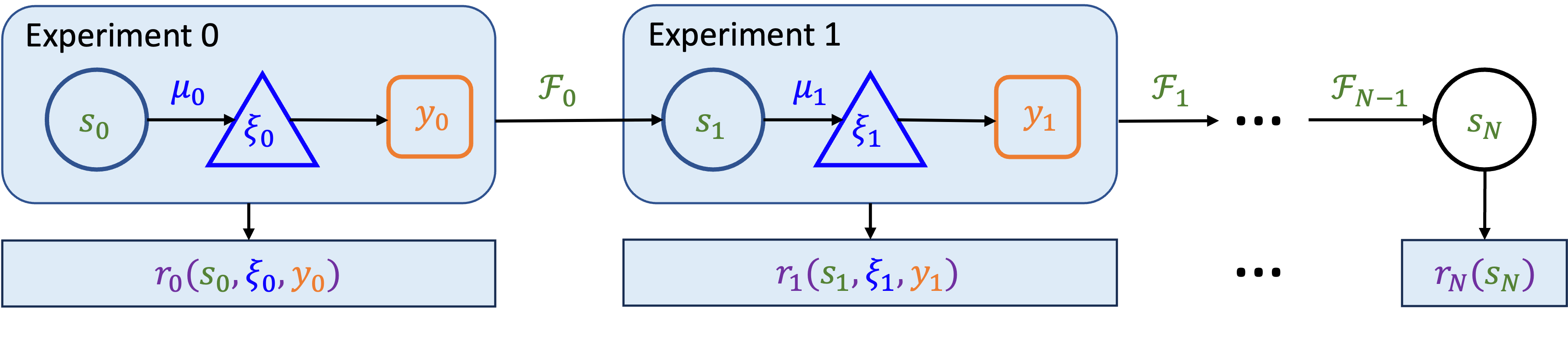
Figure 5.1: In the MDP progression of sequential experimental design, we start with an initial state $s_{0}$ (i.e., initial prior and physical state), evaluate the policy function at the state $\mu_{0}(s_{0})$ to obtain the design $\xi_{0}$ for experiment 0, conduct the experiment to obtain its outcome $y_{0}$ and immediate reward $r_{0}(s_{0},\xi_{0},y_{0})$, update the state to the new state via the transition dynamics $s_{1}=\mathcal{F}_{0}(s_{0},\xi_{0},y_{0})$ (i.e., updated posterior and physical state), and repeat for the next experiments. Once the last experiment $N-1$ is completed, the terminal state $s_{N}=\mathcal{F}_{N-1}(s_{N-1},\xi_{N-1},y_{N-1})$ can be computed along with the corresponding terminal reward $r_{N}(s_{N})$. Figure adapted from Shen and Huan (2023).

5.3 Problem statement

The sOED problem entails finding a design policy $\pi^{\ast}$ that maximizes the expected utility $U(\pi)$:

$$\pi^{\ast}\in\operatornamewithlimits{argmax}_{\pi=\{\mu_{0},\ldots,\mu_{N-1}\}} \ \ \left\{U(\pi)\coloneqq\mathbb{E}_{Y_{0:N-1}|\pi,s_{0}}\left[\sum_{k=0}^{N-1}r_{k}(S_{k},\xi_{k},Y_{k})+r_{N}(S_{N})\right]\right\}$$ (103)

subject to $$\ \ \ \xi_{k}=\mu_{k}(S_{k})\in\mathcal{A}_{k},$$

$$\ \ \ S_{k+1}=\mathcal{F}_{k}(S_{k},\xi_{k},Y_{k}),\quad\text{for}\,\,k=0,\dots,N-1.$$

Here $Y_{0:N-1}=Y_{0},Y_{1},\ldots,Y_{N-1}$. The initial state $s_{0}$ is assumed known; if it is not known, then another expectation can be taken over the random initial state $S_{0}$. Optionally, a discount factor $\gamma\in(0,1]$ can multiply the reward at each successive stage (hence yielding terms $\gamma^{k}r_{k}$) to artificially reduce the value of rewards obtained further in the future. The expected utility here is also known as the expected return (or expected total reward) in MDP terminology; we will use these terms interchangeably.

In the field of reinforcement learning (Kaelbling et al. 1996, Sutton and Barto 2018), problem (103) corresponds to a model-based planning problem, described by a finite-horizon belief-state MDP with continuous action and observation spaces. Embedded in each transition $\mathcal{F}_{k}$ is a step of Bayesian inference, which can be quite expensive to perform, especially in nonlinear and non-Gaussian settings with computationally intensive likelihoods.

5.4 Solution approaches

In general, problem (103) cannot be solved analytically. Different numerical strategies must be adopted to find an approximate solution. Before we highlight representative approaches from recent literature, we introduce two types of value function that are central to the MDP formulation, as many solution strategies are built on approximating these functions.

The action-value functions (or Q-functions) corresponding to a policy $\pi$ are

$$Q_{k}^{\pi}(s_{k},\xi_{k}) =\mathbb{E}_{Y_{k:(N-1)}|\pi,s_{k},\xi_{k}}\left[r_{k}(s_{k},\xi_{k},Y_{k})+\sum_{t=k+1}^{N-1}r_{t}(S_{t},\mu_{t}(S_{t}),Y_{t})+r_{N}(S_{N})\right]$$ (104)

$$=\mathbb{E}_{Y_{k}|\pi,s_{k},\xi_{k}}\left[r_{k}(s_{k},\xi_{k},Y_{k})+Q^{\pi}_{k+1}(S_{k+1},\mu_{k+1}(S_{k+1}))\right],$$ (105)

for $k=0,\ldots,N-1$ and subject to $S_{t+1}=\mathcal{F}_{t}(S_{t},\xi_{t},Y_{t})$, with $Q_{N}^{\pi}(s_{N})=r_{N}(s_{N})$. The value of the Q-function $Q_{k}^{\pi}(s_{k},\xi_{k})$ is the expected remaining cumulative reward (i.e., the expected sum of all remaining rewards) for performing the $k$th experiment at design $\xi_{k}$ from state $s_{k}$ and thereafter following policy $\pi$.

The state-value functions (or V-functions) corresponding to a policy $\pi$ are

$$V_{k}^{\pi}(s_{k}) =\mathbb{E}_{Y_{k:(N-1)}|\pi,s_{k}}\left[r_{k}(s_{k},\mu_{k}(s_{k}),Y_{k})+\sum_{t=k+1}^{N-1}r_{t}(S_{t},\mu_{t}(S_{t}),Y_{t})+r_{N}(S_{N})\right]$$ (106)

$$=\mathbb{E}_{Y_{k}|\pi,s_{k}}\left[r_{k}(s_{k},\mu_{k}(s_{k}),Y_{k})+V^{\pi}_{k+1}(S_{k+1})\right],$$ (107)

for $k=0,\ldots,N-1$ and subject to $S_{t+1}=\mathcal{F}_{t}(S_{t},\xi_{t},Y_{t})$, with $V_{N}^{\pi}(s_{N})=r_{N}(s_{N})$. The value of the V-function $V_{k}^{\pi}(s_{k})$ is the expected remaining cumulative reward starting from a given state $s_{k}$ and following policy $\pi$ for all remaining experiments. The expected utility in (103) can be succinctly written as $U(\pi)=V_{0}^{\pi}(s_{0})$.

The V-function and Q-function are related to each other via

$$V_{k}^{\pi}(s_{k})=Q_{k}^{\pi}(s_{k},\mu_{k}(s_{k})),$$ (108)

and thus often only one of the two value functions needs to be solved for. We note that both value functions can also be expressed in the recursive forms (105) and (107). When the policy is the optimal policy $\pi^{\ast}$ from (103), the recursive relations become the well-known Bellman optimality equations:

$$V_{k}^{\ast}(s_{k}) =\max_{\xi_{k}\in\mathcal{A}_{k}}\mathbb{E}_{Y_{k}|\xi_{k},s_{k}}\left[r_{k}(s_{k},\xi_{k},Y_{k})+V^{\ast}_{k+1}(S_{k+1})\right],$$ (109)

$$V_{N}^{\ast}(s_{N}) =r_{N}(s_{N}),$$ (110)

for $k=0,\ldots,N-1$. In this form, the optimal policy $\pi^{\ast}$ is expressed implicitly, since the designs selected by $\pi^{\ast}$ are maximizers of (109).

Furthermore, if the reward terms are chosen to create the sequential analogue of $u^{\text{div}}$ in (20)—i.e., to capture the total expected information gain (EIG) in the model parameter $\Theta$ from all experiments—two natural formulations arise. A terminal formulation places in the terminal reward a single Kullback–Leibler (KL) divergence from the initial prior to the final posterior:

$$r_{k}(s_{k},\xi_{k},y_{k}) =0,\quad k=0,\ldots,N-1,$$ (111)

$$r_{N}(s_{N}) =D_{\text{KL}}\left(p_{\Theta|\kern 0.35002pt{\sf i}_{N}}||p_{\Theta}\right).$$ (112)

An incremental formulation instead captures all incremental KL divergence terms from each intermediate experiment’s prior to its corresponding posterior:

$$r_{k}(s_{k},\xi_{k},y_{k}) =D_{\text{KL}}\left(p_{\Theta|\kern 0.35002pt{\sf i}_{k+1}}||p_{\Theta|\kern 0.35002pt{\sf i}_{k}}\right),\quad k=0,\ldots,N-1,$$ (113)

$$r_{N}(s_{N}) =0.$$ (114)

As pointed out in Theorem 1 of Shen and Huan (2021, 2023) and Theorem 1 of Foster et al. (2021), the expected utility $U_{T}(\cdot)$ produced by substituting (111)–(112) into (103), and the expected utility $U_{I}(\cdot)$ produced by substituting (113)–(114) into (103), are equal: $U_{T}(\pi)=U_{I}(\pi)$, for any given policy $\pi$. We can also show this equality using the chain rule of mutual information. Starting from the incremental formulation, each immediate reward’s contribution to (103) is

$$\mathbb{E}_{Y_{0:N-1}|\pi,s_{0}}\left[D_{\text{KL}}\left(p_{\Theta|\kern 0.35002ptI_{k+1}}||p_{\Theta|\kern 0.35002ptI_{k}}\right)\right]$$

$$=\mathbb{E}_{Y_{0:k-1}|\pi,s_{0}}\,\mathbb{E}_{Y_{k}|Y_{0:k-1},\pi,s_{0}}\left[\mathbb{E}_{\Theta|\kern 0.35002ptI_{k+1}}\left[\log\frac{p(\Theta|\kern 0.50003ptI_{k+1})}{p(\Theta|{I_{k}})}\right]\right]$$

$$=\mathbb{E}_{Y_{0:k-1}|\pi,s_{0}}\,\mathbb{E}_{\Theta,Y_{k}|\xi_{k},I_{k}}\left[\log\frac{p(\Theta,Y_{k}|\xi_{k},{I_{k}})}{p(\Theta|{I_{k}})p(Y_{k}|\xi_{k},{I_{k}})}\right]$$

$$=\mathbb{E}_{Y_{0:k-1}|\xi_{0:k-1}}\left[D_{\text{KL}}\left(p_{\Theta,Y_{k}|\xi_{k},I_{k}}||p_{\Theta|\kern 0.35002ptI_{k}}\otimes p_{Y_{k}|\xi_{k},I_{k}}\right)\right]$$

$$=\mathcal{I}(\Theta;Y_{k}|\xi_{k},{I_{k}}),$$ (115)

where all $\xi_{k}$ follow from the given policy $\pi$. In the first equality above, the expectation over $Y_{k+1:N-1}$ collapses since the immediate reward does not depend on these observations. In the second equality, we use the fact that

$$\mathbb{E}_{Y_{k}|Y_{0:k-1},\pi,s_{0}}=\mathbb{E}_{Y_{k}|Y_{0:k-1},\xi_{0:k}}=\mathbb{E}_{Y_{k}|\xi_{k},I_{k}},$$

where $\xi_{k}$ follows from the policy $\pi$. Summing the conditional mutual information terms (115) according to (103) yields

$$U_{I}(\pi)=\sum_{k=0}^{N-1}\mathcal{I}(\Theta;Y_{k}|\xi_{k},{I_{k}})=\mathcal{I}(\Theta;Y_{0:N-1}|\xi_{0:N-1})=U_{T}(\pi),$$ (116)

via the chain rule of mutual information.

We note that the incremental reward functions can be augmented with additional terms, e.g., rewards reflecting the costs of candidate designs, without affecting the correspondence of these two ways of expressing total EIG.

Computationally, the terminal formulation requires only a single KL divergence estimate per trajectory, at its terminal point. (A ‘trajectory’ is a realization of the sequence of designs and observations, also known as an ‘episode’ in MDP terminology.) In contrast, the incremental formulation needs many more intermediate KL divergence calculations, which can be quite costly. On the other hand, the terminal formulation is a case of delayed reward, where the feedback from the reward occurs only at the completion of all experiments, which can make learning of the intermediate value functions more difficult. Lastly, we note that a greedy design strategy requires calculating all intermediate posteriors and KL divergence terms, which is computationally much more expensive than the sOED terminal formulation.

5.4.1 Approximate dynamic programming (ADP-sOED)

While approximate dynamic programming (ADP) can refer to a range of computational techniques for finding an optimal policy (Powell 2011), we refer here to the approach introduced in Huan (2015) and Huan and Marzouk (2016), which centers on the idea of numerically approximating the optimal V-functions $V_{k}^{\ast}(s_{k})$ that satisfy the Bellman optimality equations (109) and (110), using some parametrized $\tilde{V}_{k}^{\ast}(s_{k})$. We call this method ADP-sOED.

In their work, the belief state $s_{k}^{b}$ is represented by discretizing the posterior density function on an adaptive tensor-product grid, which is expanded/shrunk and refined/coarsened based on local density values. Alternatively, Huan (2015) also explores representing all possible posterior distributions by constructing a triangular transport map (Moselhy and Marzouk 2012, Marzouk et al. 2016) jointly on $(\xi_{k},Y_{k},\Theta)$, where $\xi_{k}$ is sampled from a probability distribution with full support on $\mathcal{A}_{k}$ and $(Y_{k},\Theta)$ are drawn from the corresponding prior predictives at stage $k$. See more discussion of such constructions in Section 3.2. In either case, a linear architecture $\tilde{V}_{k}^{\ast}(s_{k})=\sum_{i=1}^{m}\beta_{k,i}\psi_{k,i}(s_{k})$ is used to approximate the optimal V-functions, where features $\psi_{k,i}(s_{k})$ are selected to be polynomial functions of the physical state and of the posterior moments.

Once the representations of $s_{k}^{b}$ and $\tilde{V}_{k}^{\ast}$ are chosen, a procedure known as approximate value iteration (also referred to as backward induction, especially for finite-horizon settings) is used to build the approximate V-functions. The main steps of the overall algorithm are summarized as follows.

1. Trajectory simulation. Generate trajectories induced by the current approximate V-functions $\tilde{V}_{k}^{\ast}$, by choosing the design $\tilde{\xi}_{k}^{\ast}$ at each stage via

   $$\tilde{\xi}_{k}^{\ast}\in\arg\max_{\xi_{k}\in\mathcal{A}_{k}}\mathbb{E}_{Y_{k}|\xi_{k},s_{k}}\left[r_{k}\left(s_{k},\xi_{k},Y_{k}\right)+\tilde{V}^{\ast}_{k+1}\left(\mathcal{F}_{k}(s_{k},\xi_{k},Y_{k})\right)\right].$$ (117)

   To realize the corresponding state trajectories $(s^{(i)}_{k})_{k=0}^{N}$ sequentially, where $i$ indexes trajectories, an observation $y_{k}^{(i)}$ is simulated at each stage using the statistical model $p\big{(}y_{k}|\theta^{(i)},\tilde{\xi}_{k}^{\ast,(i)},{\sf i}_{k}^{(i)}\big{)}$, the current design, and a realization $\theta^{(i)}$ of $\Theta$ generated from the prior at $k=0$ and then fixed for that entire trajectory; in other words, $\theta^{(i)}$ serves as the true value of $\Theta$ for that trajectory. Belief states are updated using the grid or transport representations noted above. An exploration policy, which simply generates random designs, can be used if $\tilde{V}_{k+1}^{\ast}$ is not yet available, and otherwise may provide supplementary trajectory samples.

2. Approximate value iteration (backward induction). Start from the final stage $k=N-1$ and evaluate (109) at the sample states $s_{N-1}^{(i)}$ generated in step 1,

   $$\tilde{V}_{\text{tr}}^{(i)}=\max_{\xi_{k}\in\mathcal{A}_{k}}\mathbb{E}_{Y_{k}|\xi_{k},s_{k}^{(i)}}\left[r_{k}\big{(}s_{k}^{(i)},\xi_{k},Y_{k}\big{)}+\tilde{V}^{\ast}_{k+1}\big{(}\mathcal{F}_{k}\big{(}s_{k}^{(i)},\xi_{k},Y_{k}\big{)}\big{)}\right],$$ (118)

   and then use these evaluations as training points to update the approximate V-functions $\tilde{V}^{\ast}_{k}$ via linear regression:

   $$\big{\{}s_{k}^{(i)},\tilde{V}_{\text{tr}}^{(i)}\big{\}}\rightarrow\tilde{V}^{\ast}_{k}(s_{k}).$$ (119)

   Once $\tilde{V}^{\ast}_{k}$ is updated, repeat the same process stepping backwards from $k=N-2,N-3,\ldots$ to $k=0$, thus completing the update for all of the V-function approximations.

3. Refinement. Optionally repeat steps 1–2 to improve the pool of trajectory samples and hence (state, value) pairs for training, using the newly updated V-function approximations. Once iterations are terminated, a final set of functions $\tilde{V}^{\ast}_{k}$ is returned, which can be used to evaluate approximate optimal design actions through (117).

The approximation structure in (117) is known as one-step lookahead due to its invocation of an approximation function after one step of dynamic programming (Bertsekas 2005). This is not to be confused with a greedy or myopic design strategy that is based on truncating the problem horizon; doing so would not incorporate value from any future experiments beyond that truncated horizon.

It is important to note that both (117) and (119) require solving a stochastic approximation problem (e.g., using the Robbins–Monro algorithm (Robbins and Monro 1951)), since the expectation therein is typically estimated using Monte Carlo. In fact, since the policy is only implicitly represented by the V-functions, using the final policy still involves solving (117). As a result, ADP-sOED is quite computationally expensive.

5.4.2 Actor-critic policy gradient (PG-sOED)

In response to the heavy computations required by ADP-sOED, rooted in approximating the optimal V-functions in lieu of the policy, faster methods have been developed by explicitly representing the policy and extracting its gradient, generally known as policy gradient (PG) approaches (Sutton et al. 1999). One such method is the PG-based sOED (PG-sOED) introduced in Shen and Huan (2023) (and its earlier version, Shen and Huan 2021), which makes use of actor-critic techniques (Konda and Tsitsiklis 1999, Peters and Schaal 2008)—specifically, actor-critic techniques for deterministic policies with deep neural network parameterizations (Silver et al. 2014, Lillicrap et al. 2016, Mnih et al. 2015).

Suppose that each policy function $\mu_{k}$ is given a parametric representation $\mu_{k,w_{k}}$ with parameters $w_{k}$. Collecting these functions in

$$\pi_{w}\coloneqq\{\mu_{0,w_{0}},\mu_{1,w_{1}},\ldots,\mu_{N-1,w_{N-1}}\}\quad\text{with}\quad w\coloneqq\{w_{0},w_{1},\ldots,w_{N-1}\},$$

the sOED problem searching within the new parameterized policy space now entails solving

$$\max_{w}U(\pi_{w}).$$

An expression for the policy gradient can be derived (Shen and Huan 2023, Theorem 2):

$$\nabla_{w}U(\pi_{w})=\sum_{k=0}^{N-1}\mathbb{E}_{Y_{k}|\pi_{w},s_{0}}\left[\nabla_{w}\mu_{k,w_{k}}(S_{k})\nabla_{\xi_{k}}Q_{k}^{\pi_{w}}(S_{k},\xi_{k})\right]$$ (120)

with $\xi_{k}=\mu_{k,w_{k}}(S_{k})$ and $S_{k+1}=\mathcal{F}_{k}(S_{k},\xi_{k},Y_{k})$. The appearance of $\nabla_{\xi_{k}}Q_{k}^{\pi_{w}}$ in (120) further motivates a parameterization of the Q-functions, similarly denoted by

$$Q^{\pi_{w}}_{\eta}\coloneqq\big{\{}Q^{\pi_{w}}_{0,\eta_{0}},Q^{\pi_{w}}_{1,\eta_{1}},\ldots,Q^{\pi_{w}}_{N,\eta_{N}}\big{\}}\quad\text{with}\quad\eta\coloneqq\{\eta_{0},\eta_{1},\ldots,\eta_{N}\}.$$

Simultaneously learning the parameterized policy (the actor $\pi_{w}$) and the Q-functions (the critic $Q^{\pi_{w}}_{\eta}$) makes this an actor-critic method. Overall, access to the policy gradient opens the door to a wide range of gradient-based optimization methods to iteratively improve the policy $\pi_{w}$ en route to maximizing $U(\pi_{w})$.

To this end, Shen and Huan (2023) use the policy gradient to develop several numerical methods for solving (103). In what follows, the background information sequence $I_{k}$ is always used to represent the state, as discussed in Section 5.2. First, a Monte Carlo estimator of (120) is formed via

$$\nabla_{w}U(\pi_{w})\approx\frac{1}{M}\sum_{i=1}^{M}\sum_{k=0}^{N-1}\nabla_{w}\mu_{k,w_{k}}\big{(}s^{(i)}_{k}\big{)}\nabla_{\xi_{k}}Q^{\pi_{w}}_{k}\big{(}s^{(i)}_{k},\xi^{(i)}_{k}\big{)}$$ (121)

with $\xi^{(i)}_{k}=\mu_{k,w_{k}}\big{(}s^{(i)}_{k}\big{)}$ computed from the current policy. Here for the $i$th trajectory, a ‘true’ data-generating $\theta^{(i)}$ is drawn from the prior $s_{0}^{b}$ and used to generate all subsequent $y_{k}^{(i)}$ via the models $p\big{(}y_{k}|\theta^{(i)},\xi_{k}^{(i)},{\sf i}_{k}^{(i)}\big{)}$ for that entire trajectory.

Second, deep neural networks (DNNs) are used to parameterize both the policy and the Q-functions, following the ideas of deep Q-networks (DQN) (Mnih et al. 2015) and deep deterministic policy gradient (DDPG) (Lillicrap et al. 2016). The policy $\pi_{w}$, and hence all $\mu_{k,w_{k}}$ for $k=0,\ldots,N-1$, are represented by a single DNN called the policy network. The consolidated policy network has an input layer that takes in the state, specifically in the form of the information sequence ${\sf i}_{k}$ and the current experimental stage $k$, as depicted in Figure 5.2. The stage $k$ can be represented either directly as an integer or via its one-hot encoding (i.e., a unit vector in $\mathbb{R}^{N}$). Designs $\xi_{t}$ and observations $y_{t}$ for future experiments that have not yet taken place ($t\geq k$) are padded with zeros. The output layer returns $\xi_{k}$. The gradient of such a DNN-based policy, which is needed to evaluate (121), can be computed efficiently via back-propagation. Note that the policy network is therefore not trained in a supervised learning manner, but rather by improving $w$ en route to maximizing $U(\pi_{w})$ in solving (103).

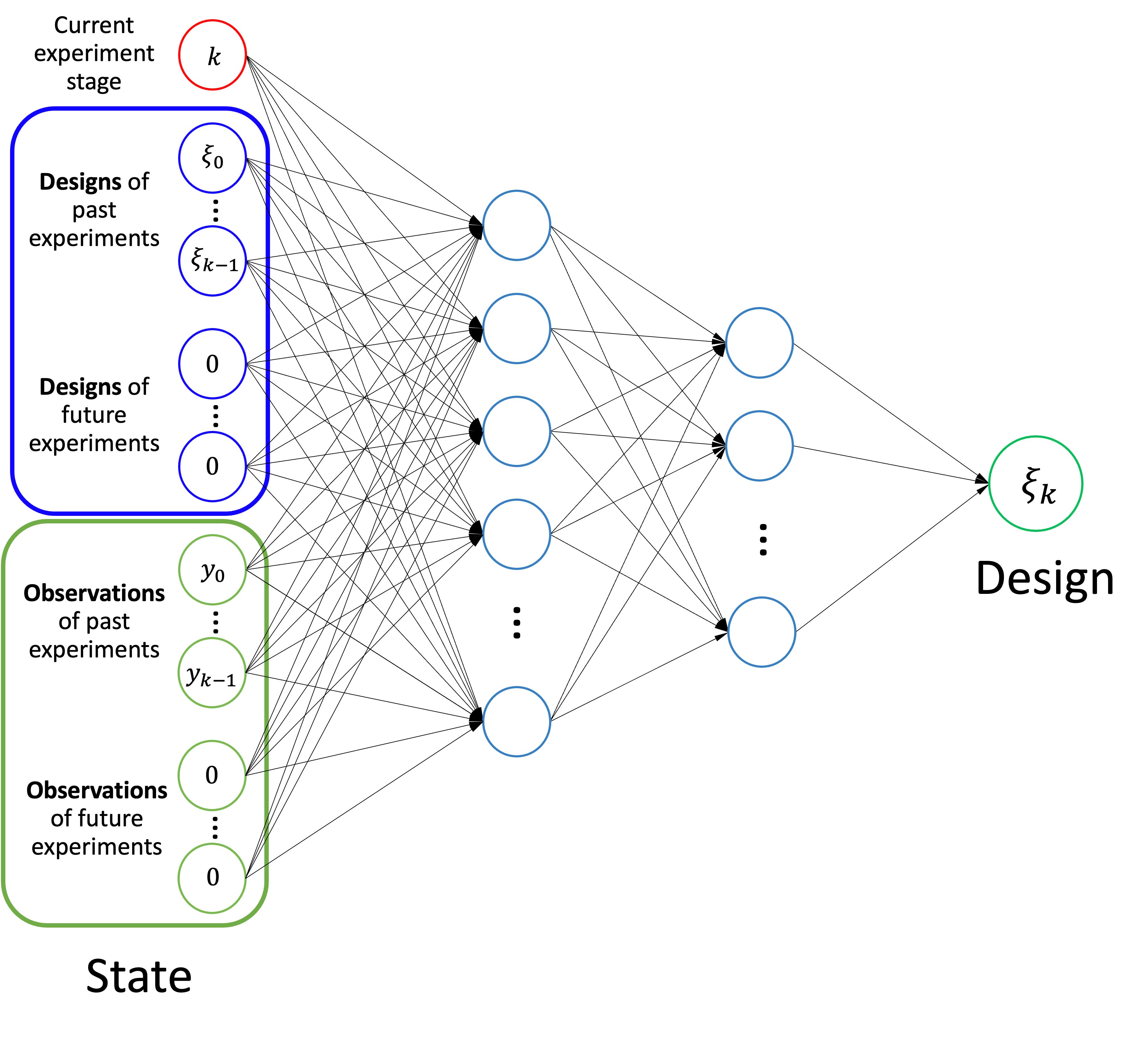
Figure 5.2: A policy is a mapping from state to design. In this DNN representation of the policy, its input entails the current experiment stage, and designs of past experiments and their resulting observations. The designs and observations of future experiments that have not yet taken place are padded with zeros.

Similarly, the consolidated Q-function $Q^{\pi_{w}}_{\eta}$ is represented by a separate, single DNN called the Q-network. The Q-network is trained in a supervised learning manner from the Monte Carlo trajectory samples by minimizing a quadratic loss derived from (105):

$$\ell(\eta)=\frac{1}{M}\sum_{i=1}^{M}\sum_{k=0}^{N-1}\left[Q^{\pi_{w}}_{k,\eta_{k}}\big{(}s^{(i)}_{k},\xi^{(i)}_{k}\big{)}-\left(r_{k}\big{(}s^{(i)}_{k},\xi^{(i)}_{k},y^{(i)}_{k}\big{)}+Q^{\pi_{w}}_{k+1}\big{(}s^{(i)}_{k+1},\xi^{(i)}_{k+1}\big{)}\right)\right]^{2}$$ (122)

with $\xi^{(i)}_{k}=\mu_{k,w_{k}}\big{(}s^{(i)}_{k}\big{)}$ computed from the current policy. Note that the last term in (122), $Q^{\pi_{w}}_{k+1}\big{(}s^{(i)}_{k+1},\xi^{(i)}_{k+1}\big{)}$, is the true Q-function as defined in (104) and thus does not depend on $\eta$. The true Q-function is usually not available, however, and therefore this term is typically replaced by the Q-function approximation at the current iteration, $Q^{\pi_{w}}_{k+1,\eta_{k+1}}\big{(}s^{(i)}_{k+1},\xi^{(i)}_{k+1}\big{)}$, but with its contribution to the $\eta$-gradient of the loss in (122) ignored. The trained Q-network $Q^{\pi_{w}}_{\eta}$ from (122) is then used to replace the true Q-function in evaluations of (121). Notably, this PG computation does not require evaluating gradients of the likelihood (or the underlying simulation model) with respect to $\xi_{k}$, since the gradient operator now only needs to act on the Q-network.

Third, the information-based immediate and/or terminal rewards $r_{k}$ and $r_{N}$, which require evaluation of the KL divergence based on the belief state, are calculated by directly approximating integrals involving the relevant unnormalized densities, via numerical quadrature. This technique, however, is only practical for low-dimensional $\Theta$ (e.g., $p\leq 4$).

Assembling these numerical methods, an optimal policy is sought using gradient-based optimization such as stochastic gradient ascent. The main steps of the overall algorithm are summarized as follows.

1. Trajectory simulation. Generate trajectories. For each trajectory, first draw $\theta$ from the prior, then for each of the $k=0,\dots,N-1$ experiments in the trajectory, sequentially compute $\xi_{k}$ from the current policy and draw $y_{k}$ from its statistical model. Calculate the associated trajectory of states; for example, if using $I_{k}$ as the state, simply store ${\sf i}_{N}$, from which all ${\sf i}_{k<N}$ can be easily extracted. Compute the corresponding immediate and terminal rewards $r_{k}$ and $r_{N}$.

2. Value function update. Update the Q-network by finding an $\eta$ that minimizes the loss in (122).

3. Policy update. Estimate $\nabla_{w}U(w)$ through (121) but using the Q-network, and update the policy network through, for example, gradient ascent $w\leftarrow w+\alpha\nabla_{w}U(w)$, where $\alpha$ is the learning rate.

4. Refinement. Repeat steps 1–3 to improve the trajectory sample pool with the newly updated policy network and Q-network. Once terminated, a final policy network is returned.

Because of the many complex approximations in these algorithms, it is useful to validate them in simple settings where an optimal policy can be derived analytically. To this end, we show how ADP-sOED and PG-sOED perform on a two-experiment linear-Gaussian benchmark problem (Huan and Marzouk 2016, Shen and Huan 2023). The model is a simplified version of (4):

$$Y_{k}=\xi_{k}\Theta+\mathcal{E}_{k}$$ (123)

with $\mathcal{E}_{k}\sim\mathcal{N}(0,1^{2})$ and no physical state. The benchmark entails $N=2$ experiments, with prior $\Theta\sim\mathcal{N}(0,3^{2})$ and designs constrained to lie in $d_{k}\in[0.1,3]$. The conjugate prior ensures that all subsequent posteriors are Gaussian, following (8) and (9). The rewards are set to

$$r_{k}(s_{k},\xi_{k},y_{k}) =0,\quad k=0,1,$$ (124)

$$r_{N}(s_{N}) =D_{\text{KL}}\left(p_{\Theta|\kern 0.35002pt{\sf i}_{N}}||p_{\Theta}\right)-2\left(\log{\sigma_{N}^{2}}-\log{2}\right)^{2},$$ (125)

where $\sigma_{N}^{2}$ is the variance of the final posterior, and the additive penalty in $r_{N}$ is purposefully inserted to make the problem more challenging. A derivation of the resulting optimal policies can be found in Huan (2015, Appendix B), with $U(\pi^{\ast})\approx 0.783$.

In this particular linear-Gaussian problem, sOED is equivalent to batch OED. Upon substituting the terminal reward (125) into the sOED objective (103) and taking an expectation over $Y_{0},Y_{1}|\pi$, the objective depends explicitly only on the final posterior variance. The portion of the objective following from the KL divergence term in (125) only involves the posterior variance, as shown by (25)–(26), and the portion resulting from the penalty term in (125) only involves the posterior variance by construction. While this variance depends on the designs chosen by the policy, in the linear-Gaussian setting it is independent of the realized values of $Y_{0:N-1}$, $y_{0:N-1}$. Consequently, feedback or adaptation in response to $y_{0:N-1}$ would not affect the expected utility, and sOED and batch OED therefore coincide. See Huan (2015, Appendix B) for a detailed derivation of this equivalence.

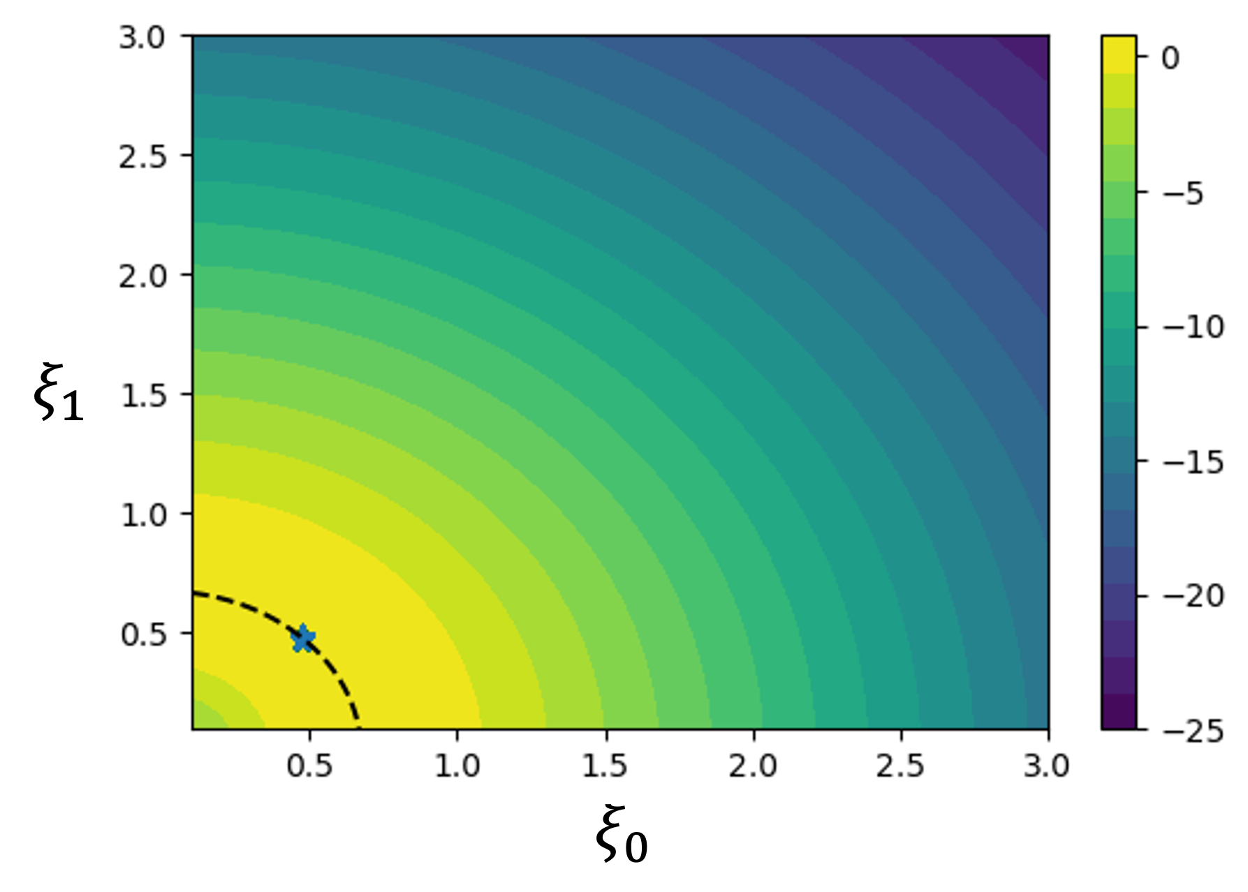
(a) ADP-sOED

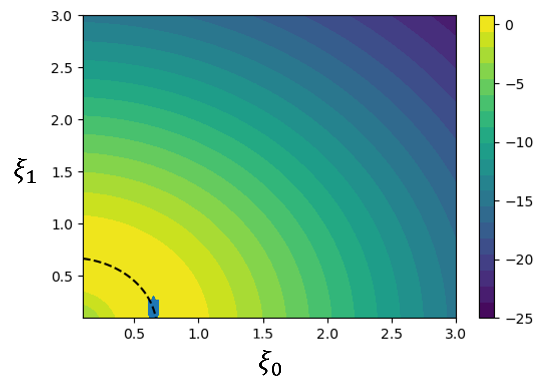
(b) PG-sOED

Figure 5.3: Expected utility contours for the linear-Gaussian benchmark with the dashed curve showing the set of optimal designs. The cluster of points in each plot indicates the designs selected by (a) ADP-sOED and (b) PG-sOED policies under repeated trials. Both algorithms arrived at the optimal set and achieved expected utility values consistent with the analytic optimal policy: $U(\pi^{\ast}_{\text{ADP}})\approx 0.775$, $U(\pi^{\ast}_{\text{PG}})\approx 0.775$, $U(\pi^{\ast})\approx 0.783$.

Figure 5.3 illustrates the expected utility for different design choices via colored contours, with the dashed curve illustrating the set of optimal designs. The cluster of points in each plot indicates the designs selected by the ADP-sOED and PG-sOED policies under repeated trials. Both algorithms arrive at the optimal set and achieve expected utility values consistent with the analytic optimal policy: $U(\pi^{\ast}_{\text{ADP}})\approx 0.775$, $U(\pi^{\ast}_{\text{PG}})\approx 0.775$, $U(\pi^{\ast})\approx 0.783$. The computational times reported in Table 5.1, adapted from Shen and Huan (2023), are obtained using a single 2.6 GHz CPU on a MacBook Pro laptop. The timing values reflect 30 gradient ascent updates for PG-sOED in the training stage, and one policy update (the minimum needed) for ADP-sOED. PG-sOED is orders of magnitude faster than ADP-sOED, especially in testing times, making it suitable for applications that have real-time requirements. This drastic difference is due to ADP-sOED being a value-based (critic-only) approach wherein the policy (actor) is not explicitly represented, such that evaluating the policy requires solving a (stochastic) optimization problem. In contrast, applying PG-sOED requires only a single forward pass through the policy network, without any additional optimization runs or forward model evaluations.

Table 5.1: Comparison of computational costs between ADP-sOED and PG-sOED for the linear-Gaussian benchmark. Data adapted from Shen and Huan (2023).

	Training time (s)	Forward model evaluations	Testing time (s)
ADP-sOED	837	$5.3\times 10^{8}$	24,396
PG-sOED	24	$3.1\times 10^{6}$	4

Figures 5.4–5.5, both adapted from Shen and Huan (2023), illustrate the application of PG-sOED to a problem of mobile sensor guidance in a two-dimensional advection-diffusion partial differential equation. The location of the center of a source term (e.g., emitting some contaminant) in the advection-diffusion problem is uncertain, along with the strength and radius of the source. Figure 5.4 shows an example of the contaminant plume concentration evolving in time, with the advection velocity pointing up and to the right. The design variables are the displacements of the mobile sensor from one stage to the next. The inference goal is to learn the unknown source location, source strength, and radius of the source, from noisy measurements of contaminant concentration at successive times. All four of these parameters are endowed with uniform priors, and the velocity field advecting the contaminant field is assumed known. The rewards for the sOED problem include the joint information gain (KL divergence from the prior to the posterior after four experiments) in all four parameters, instituted in the terminal formulation manner, along with a negative stagewise reward corresponding to a quadratic penalty on sensor movement from one stage to the next. Figure 5.5 illustrates an application of the resulting PG-sOED policy for one particular realization of the experimental sequence. The top row shows marginal posterior densities of the source location $(\Theta_{x},\Theta_{y})$, while the bottom row shows marginals of the source radius $\Theta_{h}$ and source strength $\Theta_{s}$. The movements of the sensor, i.e., the chosen designs, are visualized in the top row (red dots and lines) along with the true source location (fixed purple star).

Recall that the objective (103) being maximized involves an expectation over $\Theta$ and over all values of $Y_{0:N-1}$ realized under the policy. While Figure 5.5 shows a single trajectory of experiments, a policy is designed to work well, on average, over all possible trajectories. Thus, the most comprehensive way of assessing the effectiveness of a policy is to study the reward it produces over many realized trajectories. Figure 5.6, adapted from Shen and Huan (2023), presents histograms of the total rewards obtained from $10^{4}$ trajectories using the batch, greedy, and PG-sOED policies. Their expected values, indicated by the vertical black lines, are respectively $U(\pi^{\ast}_{\text{batch}})\approx 2.856$, $U(\pi^{\ast}_{\text{greedy}})\approx 3.057$, and $U(\pi_{\text{PG}})\approx 3.435$, with PG-sOED achieving the highest expected reward. In this example, greedy design tends to ‘chase after’ the most recent estimate of the source location. Batch design can plan ahead and take advantage of knowing where the plume will advect in future experiments, but is unable to adapt to new measurements. PG-sOED can do both.

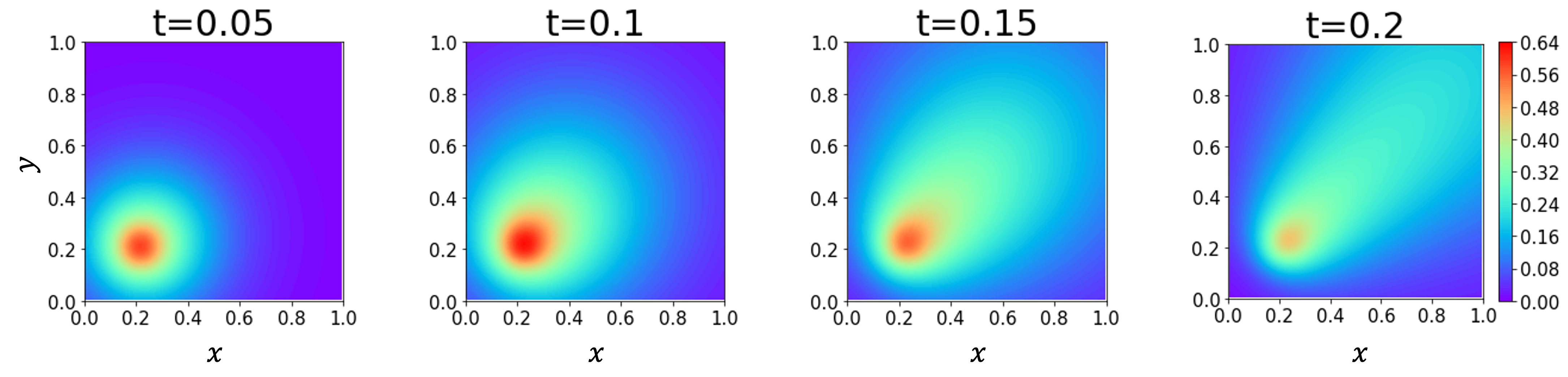
Figure 5.4: An example time-evolution of a convection-diffusion field. The contours show the concentration of the plume. Figure adapted from Shen and Huan (2023).

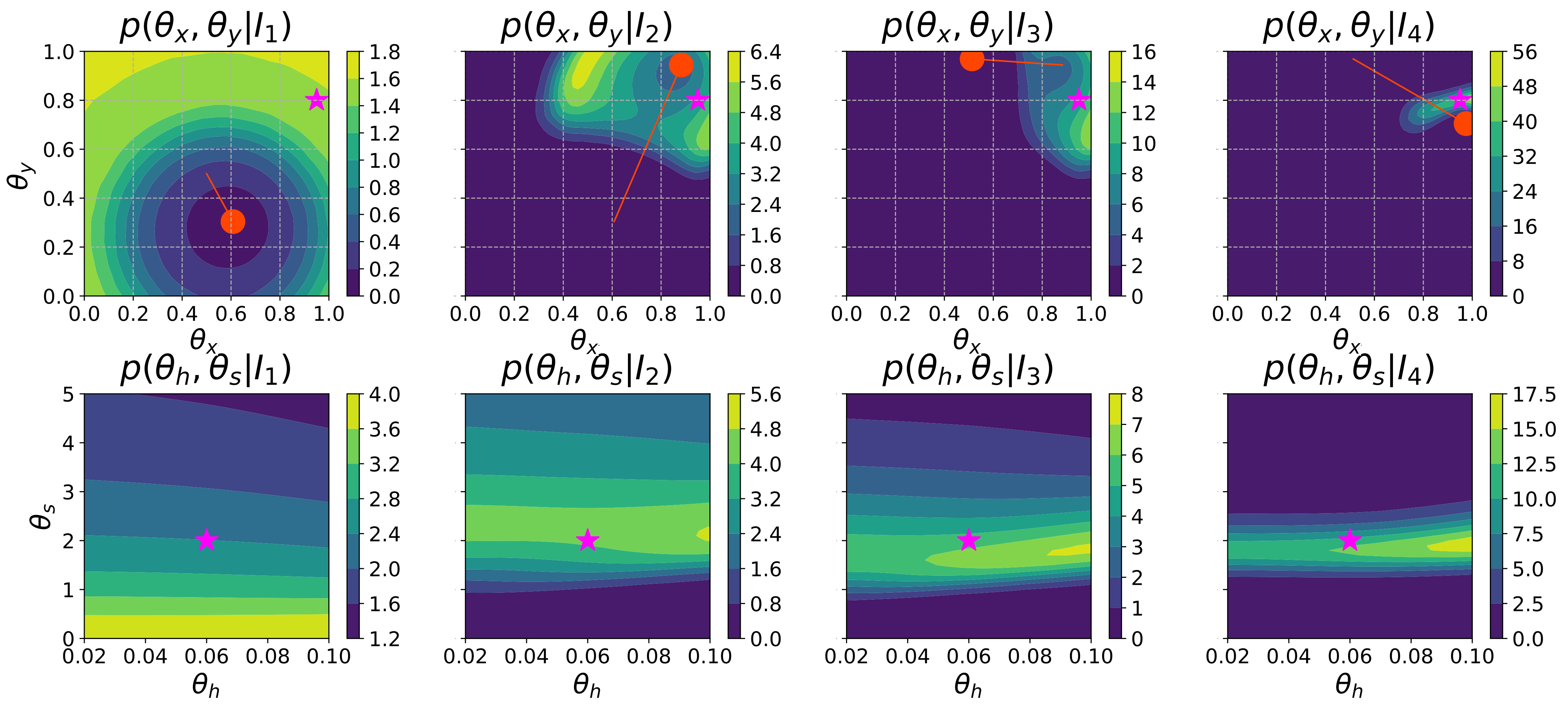
Figure 5.5: Sequence of marginal posterior densities (unknown source locations $\Theta_{x},\Theta_{y}$ on the first row, unknown source width and strength $\Theta_{h},\Theta_{s}$ on the second row) from an example trajectory instance using PG-sOED. The purple star represents the true data-generating $\theta$ value, the red dot represents the physical state (sensor location), and the red line segment depicts the design, which is the displacement of the sensor from its previous location. Figure adapted from Shen and Huan (2023).

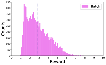
(a) Batch

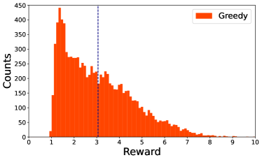
(b) Greedy

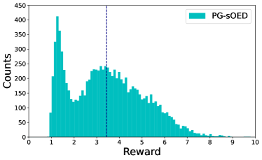
(c) PG-sOED

Figure 5.6: Histograms of total rewards from $10^{4}$ test trajectories generated using batch, greedy, and PG-sOED policies, with respective expected total reward values (indicated by vertical lines) $U(\pi^{\ast}_{\text{batch}})\approx 2.856$, $U(\pi^{\ast}_{\text{greedy}})\approx 3.057$, and $U(\pi_{\text{PG}})\approx 3.435$. Figure adapted from Shen and Huan (2023).

5.4.3 Methods that leverage information bounds

Another prominent series of sequential experimental design algorithms, developed around the same time as those discussed in Section 5.4.2, leverage various information bounds. Here we briefly summarize these methods.

DAD and related methods.

Foster et al. (2021) introduced a technique they named deep adaptive design (DAD). Like PG-sOED, DAD performs the bulk of its computation offline, constructing a DNN-based policy that can quickly produce the next design online as data are realized. Unlike PG-sOED, however, DAD does not use an actor-critic approach. For a discussion of the relative merits of actor-critic algorithms and more direct PG approaches, see Konda and Tsitsiklis (1999) and Sutton and Barto (2018, Chapter 13). The expected utility $U(\pi)$ in DAD is the total EIG in the parameters $\Theta$ from prior to posterior after $N$ experiments, which we call $U_{\text{KL}}(\pi)$ and is equivalent to the mutual information $\mathcal{I}(Y_{0:N-1};\Theta|\pi)$. DAD directly targets maximization of the EIG, by first expressing it in terms of log-density ratio of the observations $Y_{0:N-1}$, that is,

$$U_{\text{KL}}(\pi)=\mathcal{I}(Y_{0:N-1};\Theta|\pi) =\mathbb{E}_{Y_{0:N-1}|\pi,s_{0}}\left[D_{\text{KL}}(p_{\Theta|\kern 0.35002ptI_{N}}||p_{\Theta})\right]$$

$$=\mathbb{E}_{Y_{0:N-1}|\Theta,\pi,s_{0}}\mathbb{E}_{\Theta}\left[\log\frac{p(Y_{0:N-1}|\Theta,\xi_{0:N-1})}{p(Y_{0:N-1}|\xi_{0:N-1})}\right],$$ (126)

where $\xi_{k}=\mu_{k}(S_{k})$ follows the given policy $\pi$. A sequential version of the prior contrastive estimator (PCE) (cf. (77)), called the sequential PCE (sPCE), is then introduced, taking the form:

$$\mathcal{I}(Y_{0:N-1};\Theta|\pi) \geq\mathbb{E}_{Y_{0:N-1}|\pi,\Theta_{1}}\mathbb{E}_{\Theta_{1}}\mathbb{E}_{\Theta_{2:M}}\left[\log\frac{p(Y_{0:N-1}|\Theta_{1},\xi_{0:N-1})}{\frac{1}{M}\sum_{j=1}^{M}p(Y_{0:N-1}|\Theta_{j},\xi_{0:N-1})}\right]$$

$$\eqqcolon\mathcal{L}^{\text{sPCE}}(\pi;M),$$ (127)

where $\Theta_{1}$ is the data-generating parameter for $\xi_{0:N-1},Y_{0:N-1}$ in the equation above with $\xi_{k}=\mu_{k}(S_{k})$ following the given policy $\pi$; the subscripts for $Y$ and $\xi$ refer to the experiment (stage) index, while those for $\Theta$ refer to the multi-sample index of sPCE as introduced in Section 3.3.2. The key here is that the value of the data-generating $\Theta_{1}$ is included in the Monte Carlo estimate of the evidence in the denominator; including this value ensures that (127) is a lower bound to $\mathcal{I}(Y_{0:N-1};\Theta|\pi)$ for any $\pi$, which becomes tight as $M\to\infty$ (Foster et al. 2021, Theorem 2). (When $\Theta_{1}$ is excluded from the evidence estimate, (127) reverts to the standard nested Monte Carlo estimator of EIG.) Approximating the expectations in sPCE with Monte Carlo sampling from the prior and from the statistical models for successive $(Y_{k})_{k=0}^{N-1}$ yields in the end a negatively biased Monte Carlo estimator of $\mathcal{I}(Y_{0:N-1};\Theta|\pi)$.

When the policy $\pi$ is parameterized as $\pi_{w}$, DAD seeks a policy that satisfies

$$\max_{w}\mathcal{L}^{\text{sPCE}}(\pi_{w};M).$$

The gradient of the sPCE bound can be obtained by moving the gradient operator $\nabla_{w}$ inside the expectations. This may require first reparameterizing the stochasticity in the observations to be independent of the policy. (For instance, with a statistical model $Y_{k}=G_{k}(\Theta,\xi_{k})+\mathcal{E}_{k}$, an expectation over $Y_{k}$ can be rewritten as an expectation over $\mathcal{E}_{k}$; if the distribution of $\mathcal{E}_{k}$ is functionally independent of the design $\xi_{k}$, then the goal is already achieved. More generally, if the distribution of $\mathcal{E}_{k}$ does depend on $\xi_{k}$, then the expectation can always be rewritten in terms of some other random variable whose distribution is independent of $\xi_{k}$ and hence of $\pi$.) The sPCE gradient is then

$$\nabla_{w}\mathcal{L}^{\text{sPCE}}(\pi_{w};M)=\mathbb{E}_{\mathcal{E}_{1:N}}\mathbb{E}_{\Theta_{1:M}}\left[\nabla_{w}\left(\log\frac{p(Y_{0:N-1}|\Theta_{1},\xi_{0:N-1})}{\frac{1}{M}\sum_{j=1}^{M}p(Y_{0:N-1}|\Theta_{j},\xi_{0:N-1})}\right)\right]$$ (128)

with $\xi_{k}=\mu_{k,w_{k}}(S_{k})$ following the given policy $\pi_{w}$. With this gradient in hand, one can use any gradient-based optimization scheme, such as stochastic gradient ascent, to find a parameterized policy that maximizes the estimated lower bound. With regard to how to choose the parameterization $\pi_{w}$, Foster et al. (2021) recommend a ‘pooling-emitter’ DNN architecture, motivated by the permutation invariance of the EIG under certain conditions (e.g., if all the observations in the sequence are conditionally independent given the parameters, and described by the same parametric statistical model).

Blau et al. (2022) build on the sPCE bound from DAD, but seek a stochastic policy via the randomized ensembled double Q-learning approach of Chen et al. (2021), which is an actor-critic method. They demonstrate applicability of this approach to discrete design spaces.

iDAD.

All of the sequential design methods discussed so far require the ability to explicitly evaluate the likelihood (i.e., to evaluate the probability densities $p(y_{k}|\theta,\xi_{k},{\sf i}_{k})$). In certain problems, however, the likelihood may be only implicitly defined and otherwise intractable to compute; yet sampling $Y_{k}$ from the model may still be possible. To accommodate such models in sOED, a variation of DAD, called implicit deep adaptive design (iDAD), has been developed by Ivanova et al. (2021).

iDAD introduces several likelihood-free lower bounds. The main idea behind these bounds can be understood as approximating the posterior-to-prior or likelihood-to-evidence density ratio through a parameterized ‘critic’ function, denoted here by $f:\bm{\Theta}\times\Xi_{0:N-1}\times\mathcal{Y}_{0:N-1}\rightarrow\mathbb{R}$. Note that this notion of a critic differs from the ‘critic’ in the actor-critic methods of Section 5.4.2 (where the role of the critic was played by the Q-function). In these lower bound expressions, any choice of $f$ yields a tractable lower bound for the EIG; thus $f$ can act as the ‘knob’ to maximize the lower bound. One example is the sequential design version of the NWJ bound (cf. (75))

$$\mathcal{I}(Y_{0:N-1};\Theta|\pi) \geq\mathbb{E}_{\Theta}\mathbb{E}_{Y_{0:N-1}|\Theta,\pi}\left[f(\Theta,I_{N})\right]-\frac{1}{e}\mathbb{E}_{Y_{0:N-1}|\pi}\mathbb{E}_{\Theta}\left[\exp f(\Theta,I_{N})\right]$$

$$\eqqcolon\mathcal{L}^{\text{sNWJ}}(\pi;f),$$ (129)

while another is the InfoNCE bound (cf. (79))

$$\mathcal{I}(Y_{0:N-1};\Theta|\pi) \geq\mathbb{E}_{\Theta_{1}}\mathbb{E}_{Y_{0:N-1}|\Theta_{1},\pi}\mathbb{E}_{\Theta_{2:M}}\left[\log\frac{\exp f(\Theta_{0},I_{N})}{\frac{1}{M}\sum_{j=1}^{M}\exp f(\Theta_{j},I_{N})}\right]$$

$$\eqqcolon\mathcal{L}^{\text{sNCE}}(\pi;M,f).$$ (130)

Both bounds can be tight for an optimal selection of the critic function $f$ and as $M\rightarrow\infty$ (Ivanova et al. 2021). Importantly, these bounds no longer involve the densities $p(y_{k}|\theta,\xi_{k},{\sf i}_{k})$. Upon parameterizing the policy $\pi$ as $\pi_{w}$ and critic $f$ as $f_{\phi}$, a policy can be found by maximizing (tightening) the lower bound simultaneously over $w$ and $\phi$. For example, in the NWJ case:

$$\max_{w,\phi}\mathcal{L}^{\text{sNWJ}}(\pi_{w};f_{\phi}).$$

Similar to DAD, the gradient of the lower bound with respect to both the policy and critic parameters can be obtained by bringing the gradient inside the expectation upon reparameterizing the observations, allowing for stochastic gradient ascent updates to tighten the bound. We note that while iDAD does not require explicit likelihoods and relies only on a simulator of $Y_{k}$, it does require access to derivatives of the output of this simulator with respect to the design $\xi_{k}$, and with respect to all previous experiments’ designs and outcomes, ${\sf i}_{k}$.

vsOED.

The variational sequential OED (vsOED) method in Shen et al. (2023) derives a lower bound for the EIG by employing variational approximations of the relevant posterior distributions and then substituting these approximations in ‘one-point’ reward functions that replace the KL divergence rewards, which we shall describe below. The framework generalizes the objective functions used in previous approaches in that it simultaneously accommodates multiple models, nuisance parameters, predictive quantities of interest, and implicit likelihoods.

Let $\mathcal{M}_{m}$ be a countable set of models indexed by $m=1,2,\ldots$, where each model has its own parameters $\Theta_{m}\in\bm{\Theta}_{m}\subseteq\mathbb{R}^{p_{m}}$ and predictive quantity of interest (QoI) $Z_{m}=\Psi_{m}(\Theta_{m})$, with $\Psi_{m}:\bm{\Theta}_{m}\rightarrow\mathbb{R}^{q_{m}}$ for some $q_{m}\leq p_{m}$. Suppose also that we have a prior distribution $P_{M}(m)$ over the model indicator $M$, a prior $p_{\Theta_{m}}(\theta_{m}|m)$ for the parameters $\Theta_{m}$ of each model, and a prior $p_{Z_{m}}(z_{m})$ for each model’s QoI $Z_{m}$ induced by $p_{\Theta_{m}}$ and $\Psi_{m}$. A combined reward function that includes a weighted combination of information gains in these random variables can then be formed. For example, the incremental formulation in (113) and (114) becomes

$$r_{k}(s_{k},\xi_{k},y_{k}) =\alpha_{M}D_{\text{KL}}\left(P_{M|\kern 0.35002pt{\sf i}_{k+1}}||P_{M|\kern 0.35002pt{\sf i}_{k}}\,\right)$$

$$\quad+\mathbb{E}_{M|\kern 0.35002pt{\sf i}_{k+1}}\Big{[}\alpha_{\Theta}D_{\text{KL}}\left(p_{\Theta_{m}|\kern 0.35002pt{\sf i}_{k+1}}||p_{\Theta_{m}|\kern 0.35002pt{\sf i}_{k}}\right)$$

$$\hskip 35.00005pt+\alpha_{Z}D_{\text{KL}}\left(p_{Z_{m}|\kern 0.35002pt{\sf i}_{k+1}}||p_{Z_{m}|\kern 0.35002pt{\sf i}_{k}}\right)\Big{]},\quad k=0,\ldots,N-1,$$ (131)

$$r_{N}(s_{N}) =0,$$ (132)

where $\alpha_{M}\in[0,1]$ (for the model indicator), $\alpha_{\Theta}\in[0,1]$ (for the model parameters), and $\alpha_{Z}\in[0,1]$ (for the predictive QoIs) are the weights of KL contributions from these variables. The terminal formulation can be constructed in a similar manner.

To compute the sOED objective in (103) with the rewards (131) and (132), an expectation needs to be taken over $Y_{0:N-1}|\pi,s_{0}$. A natural approach entails generating samples of trajectories. Consider the following procedure for trajectory generation. First, a model indicator and corresponding parameter value are drawn from the priors,

$$m_{0}\sim P_{M},\quad\theta_{m,0}\sim p\big{(}\theta_{m,0}|m_{0}\big{)},$$

with a corresponding QoI sample

$$z_{m,0}=\Psi_{m_{0}}\big{(}\theta_{m,0}\big{)}.$$

Then, $m_{0}$ and $\theta_{m,0}$ generate a trajectory ${\sf i}_{N}$ using the policy $\pi$ and the statistical models for each $Y_{k}$. A key insight is that, for any such trajectory ${\sf i}_{N}$, we know exactly the ‘oracle’ values of the model indicator and model parameters that generated the trajectory. New ‘one-point’ reward functions (which avoid the integration involved in computing the incremental KL divergence) can be constructed using these oracle values:

$$\tilde{r}_{k}(s_{k},\xi_{k},y_{k},m_{0},\theta_{m,0},z_{m,0}) =\alpha_{M}\log\frac{P(m_{0}|\kern 0.50003pt{\sf i}_{k+1})}{P(m_{0}|\kern 0.50003pt{\sf i}_{k})}+\alpha_{\Theta}\log\frac{p(\theta_{m,0}|\kern 0.50003pt{\sf i}_{k+1})}{p(\theta_{m,0}|\kern 0.50003pt{\sf i}_{k})}$$

$$\hskip 10.00002pt+\alpha_{Z}\log\frac{p(z_{m,0}|\kern 0.50003pt{\sf i}_{k+1})}{p(z_{m,0}|\kern 0.50003pt{\sf i}_{k})},\hskip 7.5ptk=0,\ldots,N-1,$$ (133)

$$\tilde{r}_{N}(s_{N},m_{0},\theta_{m,0},z_{m,0}) =0,$$ (134)

where the arguments $m_{0},\theta_{m,0},z_{m,0}$ are constrained to be the oracle values that correspond to the trajectory ${\sf i}_{k+1}=({\sf i}_{k},\xi_{k},y_{k})$ (as represented by $s_{k},\xi_{k},y_{k}$ in this notation). Computing the expected utility $\tilde{U}_{\text{KL}}$ produced by the rewards $(\tilde{r}_{k})_{k=0}^{N}$ thus requires taking the joint expectation over these random elements:

$$\tilde{U}_{\text{KL}}(\pi) =\mathbb{E}_{M_{0},\Theta_{m,0}|s_{0}}\Bigg{[}\mathbb{E}_{Y_{0:N-1}|\pi,s_{0},M_{0},\Theta_{m,0}}\Bigg{[}\sum_{k=0}^{N-1}\tilde{r}_{k}(S_{k},\xi_{k},Y_{k},M_{0},\Theta_{m,0},Z_{m,0})$$

$$\hskip 150.00023pt+\tilde{r}_{N}(S_{N},M_{0},\Theta_{m,0},Z_{m,0})\Bigg{]}\Bigg{]},$$ (135)

where we have factored the joint expectation so that the inner conditional expectation reflects the generation of a trajectory ${\sf i}_{N}$ from a single value of $m_{0}$ and $\theta_{0}$. (Since $Z_{m,0}$ is a deterministic function of $\Theta_{m,0}$ and $M_{0}$, we drop it from the expectations. If $Z_{m,0}$ had additional independent randomness, it could be included explicitly in the outer expectation, but it is not needed for the inner conditional expectation since the trajectory ${\sf i}_{N}$ does not depend on $z_{m,0}$.) Letting $U_{\text{KL}}$ denote the expected utility produced by the original rewards $(r_{k})_{k=0}^{N}$ in (131) and (132), Shen et al. (2023, Theorem 2) show that $\tilde{U}_{\text{KL}}(\pi)=U_{\text{KL}}(\pi)$ for any policy $\pi$. In other words, using the one-point rewards does not alter the expected utility objective of the sOED problem. Note, however, that the realized utility (i.e., total reward) for any specific trajectory naturally changes when using $\tilde{r}_{k}$ instead of $r_{k}$, and consequently the overall distribution of the utility (and its higher-order moments and quantiles) will be different, even though the expectation is preserved.

Evaluating the probability terms in (133) remains a challenge. To make the computation tractable, each of the probability terms is approximated within a parameterized family of distributions—taking a variational inference approach—leading to the following variational one-point reward functions:

$$\tilde{r}_{k,\phi}(s_{k},\xi_{k},y_{k},m_{0},\theta_{m,0},z_{m,0}) =\alpha_{M}\log\frac{q(m_{0}|\kern 0.50003pt{\sf i}_{k+1};\phi_{M})}{q(m_{0}|\kern 0.50003pt{\sf i}_{k};\phi_{M})}$$

$$+\alpha_{\Theta}\log\frac{q(\theta_{m,0}|\kern 0.50003pt{\sf i}_{k+1};\phi_{\Theta_{m}})}{q(\theta_{m,0}|\kern 0.50003pt{\sf i}_{k};\phi_{\Theta_{m}})}+\alpha_{Z}\log\frac{q(z_{m,0}|\kern 0.50003pt{\sf i}_{k+1};\phi_{Z_{m}})}{q(z_{m,0}|\kern 0.50003pt{\sf i}_{k};\phi_{Z_{m}})},\quad k=0,\ldots,N-1,$$ (136)

$$\tilde{r}_{N,\phi}(s_{N},m_{0},\theta_{m,0},z_{m,0}) =0,$$ (137)

with $\phi=\{\phi_{M},\phi_{\Theta_{m}},\phi_{Z_{m}}\}$ being the variational parameters describing the approximations $q$ above. We use the notation $q_{\phi}$ to represent succinctly the complete set of approximating distributions. Letting $\mathcal{L}^{\text{vsOED}}(\pi;q_{\phi})$ denote the expected utility function obtained when using (136) and (137) and taking expectation in the same manner as (5.4.3), Shen et al. (2023, Theorem 3) show that $\mathcal{L}^{\text{vsOED}}(\pi;q_{\phi})\leq\tilde{U}_{\text{KL}}(\pi)=U_{\text{KL}}(\pi)$ for any policy $\pi$. That is, adopting the variational approximation forms a lower bound to the original expected utility (i.e., the EIG).

To solve the problem, we can use an actor-critic approach as in PG-sOED, parameterizing the policy $\pi$ as $\pi_{w}$ and the corresponding Q-function (critic) $Q^{\pi_{w}}$ as $Q_{\eta}^{\pi_{w}}$. A policy can then be found by maximizing (tightening) the lower bound simultaneously over $w$ and $\phi$:

$$\max_{w,\phi}\mathcal{L}^{\text{vsOED}}(\pi_{w};q_{\phi}).$$

(Recall that $\eta$ is not directly optimized, but updated via (122).) This can be achieved by gradient ascent updates, where gradients with respect to $w$ and $\phi$ are found following similar steps to those used to obtain (120). Notably, with the introduction of the approximating distributions $q_{\phi}$, evaluation of the reward no longer requires explicit likelihoods and thus the method can be used for implicit models. Unlike DAD and iDAD, vsOED does not require access to gradients of the log-likelihood or of an underlying simulator, due to the use of a Q-network in the same way as PG-sOED.

Test problems in Shen et al. (2023) illustrate how vsOED can handle multiple models, predictive QoIs, and implicit likelihoods. For example, Figure 5.7, adapted from that paper, compares the EIG policies obtained via several sequential experimental design approaches on a source location problem introduced in Foster et al. (2021), for a range of design horizons $N$. Results are obtained by fixing the total number of trajectory samples available to each algorithm. The policies produced by each algorithm are then re-evaluated to assess their achieved EIG using a common estimator, namely the PCE lower bound estimator.

Figure 5.7: Expected utility lower bounds achieved by various sequential experimental design policies for a source location problem. vsOED-G and vsOED-N denote the vsOED method using Gaussian mixture models and normalizing flows, respectively, as variational distributions $q$. Suffixes -T and -I indicate whether the algorithm uses the terminal or incremental formulation. Figure adapted from Shen et al. (2023).

5.5 Open questions in sequential optimal design

While the approaches discussed in this section represent promising recent advances in sequential OED, there is a need for further development in many important directions. We briefly mention a few below.

One rather immediate need is for more efficient state representations—in particular, representations of the belief state $S_{k}^{b}$ (the evolving posterior distribution) that achieve the natural ‘compression’ induced by Bayesian logic. Many of the approaches described in this section simply track $I_{k}$, which has the advantages of being trivial to update (by appending the newly arrived $\xi_{k}$ and $Y_{k}$) and free of approximation error. Moreover, $I_{k}$ contains all the information necessary to compute any intermediate and final physical states (though they may not be accessible until evaluated via the transition dynamics for the physical state). A key disadvantage of using $I_{k}$, however, is that its dimension grows linearly with $k$, i.e., the number of experiments completed. A resulting numerical difficulty can already be seen in the policy network architectures used for PG-sOED (Figure 5.2) and related methods, where the state input layer needs to accommodate a variable-length $I_{k}$. This is crudely handled by creating a layer of maximum possible size and zero-padding the inapplicable entries. The efficiency of such a padding technique degrades as the design horizon $N$ increases (i.e., there are many more stages where a large fraction of the inputs are set to zero). Additionally, an $I_{k}$ of unbounded size introduces conceptual and technical difficulties in the infinite-horizon setting.

In essence, tracking $I_{k}$—the trivial sufficient statistics of the posterior—delays engaging with the actual process of Bayesian inference and the computation of posteriors. $I_{k}$ is therefore not as ‘compressed’ as the posterior, and the correspondence of $I_{k}$ values to posterior distributions is generally non-injective (multiple $I_{k}$ may lead to the same posterior). In other words, $I_{k}$ carries additional, unnecessary information beyond that which is needed to perform the Bayesian update (Jaynes and Bretthorst 2003, Cox 1946). Using state representations that directly capture the posterior—and that simultaneously allow numerical accuracy, scalability to high-dimensional parameter spaces, and easy online updating—would therefore be quite desirable. Inspiration should arise from other research areas that must maintain efficient online posterior representations, such as sequential Bayesian inference, data assimilation, and streaming variational inference.

More broadly, more efficient and scalable computational methods are needed to realize sOED with computationally intensive models, high-dimensional parameters and data, and complex design objectives. Indeed, the development of sOED is rather new compared to batch OED, and its demonstrations have thus far been confined to rather simple formulations and models. An important goal is to expand sOED’s capabilities so that it can tackle problems of the complexity now attained in batch design studies. To this end, accurate calculations of the posterior and the associated information measures—which occur repeatedly in sOED—will need to be pushed to higher dimensions. More expressive function representations and advanced reinforcement learning techniques will be needed to improve the sample efficiency of constructing a policy.

Along these lines, there is an enormous need for numerical analysis and approximation theory in these settings. From an approximation perspective, little is known about properties of optimal policies and value functions for sOED, outside of perhaps the simplest (e.g., linear-Gaussian) cases. How smooth are these functions? Do they enjoy anisotropic dependence on their inputs? Are they well approximated by low-rank tensors, or ridge functions, or in some other format that is particularly tractable? What neural network architectures are hence most suitable? Understanding these questions is necessary to characterize the optimality gaps emerging from current ad hoc choices of representation and network architecture. This understanding will also help to create more tailored and effective policy and Q-function approximations, ideally endowed with error bounds and performance guarantees. At the same time, convergence guarantees and rates for the reinforcement learning techniques used here, namely policy gradient and actor-critic methods, should be strengthened for the case of sequential experimental design in a Bayesian setting.

There is also a need to explore more sophisticated sequential design formulations: optimal stopping of sequential experiments, interleaving of batch and sequential designs, and policies that are robust to horizon changes.

Finally, as sOED is generally more computationally demanding than simpler batch and greedy designs, it would be extremely valuable to develop ways of choosing the appropriate design strategy a priori. Here we would advocate for inexpensive ways of estimating or bounding the benefit of feedback and the benefit of lookahead, before actually solving the sOED problem, and then balancing these potential upsides with their computational costs.

6 Outlook

The preceding sections have presented a broad overview of the current state of the art in optimal experimental design (OED). Research continues in all of the threads we have discussed: (i) devising design criteria that are sufficiently expressive to capture diverse experimental goals, with complex models; (ii) estimating these criteria in efficient and structure-exploiting ways, in high dimensions and/or in the presence of strong non-Gaussianity; (iii) maximizing a chosen design criterion given different parameterizations of feasible designs, whether continuous or discrete, and developing guarantees for the associated optimization algorithms; and (iv) advancing formulations and algorithms for optimal sequential design. In this final section, we will highlight some broader questions and issues that have not yet been discussed. Many of these issues remain rather open-ended, and thus we believe they comprise fertile ground for ongoing research.

6.1 Model misspecification

OED is intrinsically model-based: all of the methods we have discussed use a statistical model, perhaps augmented with prior information, to predict the outcomes of experiments at candidate designs and to assess how these outcomes might improve knowledge of model parameters, reduce uncertainty in model-based predictions, and so on. In the general decision-theoretic terms of Section 2.2, models are needed to define the utility function $u$ and to specify the distribution $p_{Y,\Theta}$ over which we take expectations to yield the expected utility $U$.

This reliance on models gives OED great power, but raises the question of what happens when models are, inevitably, misspecified—by which we mean that our statistical model $\mathcal{M}$ (1) of the data-generating process, for any given design, does not adequately capture how the data are generated in the actual experiment. In other words, $\mathcal{M}$ might not contain the distribution that generated the observed data.

A natural way to address misspecification is simply to augment the model, so that it can more closely capture the data-generating distribution. One line of work, developed in the setting of Bayesian inverse problems, is the Bayesian approximation error approach of Kaipio and Kolehmainen (2013), Kaipio and Somersalo (2007), and Alexanderian et al. (2022), which augments the noise model—for example, in the case of additive Gaussian noise, enlarging the covariance matrix of this noise—to account for error in the forward operator. Another approach is to explicitly introduce new ‘nuisance’ parameters: rather than considering only $p(y|\theta,\xi)$, one could introduce a richer model $p(y|\theta,\eta,\xi)$, where $\eta\in\bm{H}$ are additional parameters that capture previously un-modeled phenomena, such that there exists some $(\theta^{\ast},\eta^{\ast})\in\bm{\Theta}\times\bm{H}$ for which $p(y|\theta^{\ast},\eta^{\ast},\xi)$ matches the data-generating distribution for all designs $\xi\in\Xi$. This viewpoint underlies several recent efforts, e.g., Alexanderian et al. (2022) and Sargsyan et al. (2015). Here $\eta$ could represent variability or imprecision in the placement or timing of observations, background stochasticity or uncertain initial conditions, the impact of unresolved scales, etc. In a fully Bayesian setting, the design formulation discussed following (27) is relevant: the utility function can be chosen to depend on the posterior (and prior) marginal distributions of $\theta$, with the impact of the additional uncertain parameters $\eta$ handled via integration over the prior $p(\eta)$. There are two equivalent ways of writing the posterior marginal of $\theta$:

$$p(\theta|y,\xi) =\int p(\theta,\eta|y,\xi)\,\mathrm{d}\eta,$$ (138)

$$\text{where}\quad p(\theta,\eta|y,\xi) \propto p(y|\theta,\eta,\xi)p(\theta|\eta)p(\eta),$$

and

$$p(\theta|y,\xi) \propto p(y|\theta,\xi)p(\theta),$$ (139)

$$\text{where }\quad p(y|\theta,\xi) =\int p(y|\theta,\eta,\xi)p(\eta|\theta)\,\mathrm{d}\eta.$$

In the first, we perform inference for both $\theta$ and $\eta$, then focus attention on the posterior marginal of $\theta$. In the second, we first create a marginal likelihood for $\theta$ and then perform inference with this integrated quantity.

Although these viewpoints of inference are equivalent, there are two distinct ways of modeling subsequent posterior predictions. From a standard hierarchical Bayesian perspective, the distribution of predictions $Y^{+}$ at a design $\xi^{+}$ (which may or may not be equal to $\xi$) follows from the joint posterior of $\theta$ and $\eta$:

$$p_{1}(y^{+}|\xi^{+},y,\xi)=\iint p(y^{+}|\theta,\eta,\xi^{+})\,p(\theta,\eta|y,\xi)\,\mathrm{d}\theta\,\mathrm{d}\eta.$$ (140)

In this setting, both $\theta$ and $\eta$ were uncertain before observing $y$, but since they both influenced the observed value of $y$, conditioning on this observation updates one’s knowledge of both parameters. Crucially, the unknown value of the nuisance parameter $\eta$ that influences subsequent predictions is assumed to be the same as the one that affected $y$ (just as $\theta$ is common to both stages). A different model for the predictions $Y^{+}|\xi^{+}$, however, is that they arise from an independent, newly realized $\eta$ (here called $\eta^{+}$, for emphasis) that has not been conditioned on previous observations:

$$p_{2}(y^{+}|\xi^{+},y,\xi)=\iint p(y^{+}|\theta,\eta^{+},\xi^{+})\,p(\theta|y,\xi)\,p(\eta^{+})\,\mathrm{d}\theta\,\mathrm{d}\eta^{+}.$$ (141)

Embedded inadequacy models (Sargsyan et al. 2015, 2019, Morrison et al. 2018), which view uncertainty in $\eta^{+}$ as somehow irreducible, can be understood according to this prediction model (141). This model is also somewhat related to the viewpoint in Koval et al. (2020) and Alexanderian et al. (2022). We emphasize that, in this setting, the posterior marginal $p(\theta|y,\xi)$ is the meaningful representation of uncertainty in the parameters $\theta$ resulting from an experiment, even if $\eta$ is assumed irreducible; therefore it appears in the integrand of (141). It is not meaningful to simply average the conditional posterior $p(\theta|\eta,y,\xi)$, or some functional thereof, over $p(\eta)$.

In any case, whether the goal is parameter inference, or prediction following (140) or (141), the ability to perform OED with implicit models as discussed throughout Section 3 is quite useful. In particular, the posterior marginal $p(\theta|y,\xi)$ or the marginal likelihood of $\theta$, $p(y|\theta,\xi)$ are likely part of the utility function $u$; these densities are generally intractable and thus need to be estimated from samples. If the utility involves comparing prior and posterior predictions of $Y^{+}$, then again the densities (140) and (141) are likely intractable.

The approaches just discussed, however, are at best a partial solution to the problem of model misspecification, as they essentially rely on the modeler being able to create a ‘better’ statistical model for the data. In many situations, doing so may not be feasible. Approaches to this more challenging (and general) situation are very much a subject of ongoing research. They are, at least in spirit, related to earlier work on robust Bayesian analysis, which, in the words of Berger (1994), “studies …the sensitivity of Bayesian answers to uncertain inputs.” Research on robust Bayesian methods first flourished several decades ago, but much less has been done to address the sensitivity of Bayesian OED. Some relevant analysis is found in Duong et al. (2023), which considers perturbations to the likelihood $p(y|\theta,\xi)$ (in the sense of the Kullback–Leibler divergence) and elucidates the rate at which the associated mutual information and its maximizers converge as the likelihood perturbations become smaller. In a rather different (and parametric) approach, Chowdhary et al. (2023) consider Bayesian linear inverse problems in infinite dimensions and show how to compute derivatives of the mutual information/expected information gain with respect to a finite set of ‘auxiliary’ model parameters, i.e., parameters that are held fixed during the inference procedure. Attia et al. (2023) propose a robust Bayesian A-optimal design formulation, again for linear (or linearized) models, where parametric families of prior and noise covariance matrices are specified and the design criterion is maximized for the worst-case element of these families.

Go and Isaac (2022) instead take a more general nonparametric approach to misspecification, proposing a robust OED formulation rooted in distributionally robust optimization (Rahimian and Mehrotra 2019, Kuhn et al. 2019). The robustness considered by Go and Isaac (2022) is with respect to the choice of prior $p_{\Theta}$: the authors introduce an ambiguity set specified by the Kullback–Leibler divergence, $\mathcal{Q}_{\epsilon}=\{q:D_{\text{KL}}(q||p_{\Theta})\leq\epsilon\}$, and seek the design that maximizes the worst-case mutual information, over priors drawn from $\mathcal{Q}_{\epsilon}$:

$$\xi^{\ast}=\arg\max_{\xi\in\Xi}\inf_{q_{\Theta}\in\mathcal{Q}_{\epsilon}}\mathbb{E}_{Y|\xi}\left[D_{\text{KL}}(p^{q}_{\Theta|Y,\xi}||q_{\Theta})\right],$$ (142)

where the expectation is over $Y|\xi\sim\int p(y|\theta,\xi)\,q_{\Theta}(\theta)\,\mathrm{d}\theta$ and $p^{q}_{\Theta|Y,\xi}$ denotes the posterior derived from the prior $q_{\Theta}$, i.e., $p^{q}_{\Theta|Y,\xi}(\theta|y,\xi)\propto p_{Y|\Theta,\xi}(y|\theta,\xi)q_{\Theta}(\theta)$. This problem is not directly tractable, so Go and Isaac (2022) propose an approximation that is well-behaved for sufficiently small $\epsilon$.

We suggest that there is ample opportunity for further work at this intersection of distributional robustness and OED. For instance, it is important to consider robustness to other aspects of the joint distribution $p_{Y,\Theta|\xi}$, especially the likelihood (Zhang et al. 2022) and the forward operator therein. It would also be natural to consider ambiguity sets based on other divergences or distances, e.g., Wasserstein distances. And it remains to understand how to set the radius $\epsilon$ of any such ambiguity set, and to relate this value to other information one might have about the nature of the model misspecification.

Also relevant to model misspecification, Overstall and McGree (2022) propose an extension of Bayesian decision-theoretic design that enables targeted explorations of certain aspects of model choice. Specifically, they formulate the design problem using two models, modifying the decision-theoretic formulation of Section 2.2: the utility $u$ is defined according to one model, called the ‘fitted’ model, but the distribution of $Y,\Theta|\xi$ yielding the outer expectation in (13) (which transforms the utility $u(\xi,y,\theta)$ to an expected utility $U(\xi)$) is given by an alternative model, called the ‘designer’ model. Overstall and McGree (2022) suggest several potential justifications for this formulation. For instance, computing the utility $u$ might be intractable with the model that best represents the data-generating process, but tractable with a simpler alternative model; yet it could still be beneficial to use the more accurate model for the outer expectation. Alternatively, the fitted model might be quite complex and have weak prior information; in this case, computing the outer expectation with a more simplistic but informative model could yield more decisive designs. A related formulation appears in Catanach and Das (2023).

More broadly, we note that the goal of ‘robustifying’ OED is very much related to recent efforts to formulate robust notions of inference under model misspecification (see Kleijn and van der Vaart 2012, Bochkina 2019), and can benefit from advances in this direction. These two threads are inextricably linked: a ‘robustified’ OED might do a better job of producing data, but this data must then be interpreted through a model. Reverting solely to the misspecified model for this second phase makes little sense. A multitude of interesting approaches to inference under model misspecification have been proposed in recent years, e.g., coarsened inference (Miller and Dunson 2019); power posteriors (Grünwald and van Ommen 2017); reweighing data to reduce the effect of outliers, data contamination, and other forms of misspecification (Dewaskar et al. 2023); averaging posteriors over bootstrapped datasets (Huggins and Miller 2023, Pompe and Jacob 2021); modularized inference (Carmona and Nicholls 2020, Jacob et al. 2017); and many others. It would be of interest to understand how these methods could both mitigate the impact of model misspecification on OED procedures and help to better process the resulting data.

It may also be natural to depart from reliance solely on optimality criteria and to re-introduce some flavor of randomness or space filling to designs, as a means of hedging against misspecification of the models that produced the design criterion. This approach may be of particular interest in the sequential OED setting, where model error could be assessed and to some extent quantified at each stage of experimentation, in a way that informs subsequent rounds of design.

6.2 Risk-aware design criteria

The design formulations described in Section 2.2 and addressed throughout this paper focused primarily on the expectation of a utility function $u(\xi,Y,\Theta)$, where randomness in the utility is induced by the randomness in $Y$ and $\Theta$. Yet the notion of risk (see Royset (2022) for a recent review), aimed at quantifying ‘hazard’ or undesirable outcomes, is also relevant to OED. For instance, an experimenter might be interested in characterizing—and controlling—the probability and/or severity of an experimental outcome with very low utility (e.g., low information gain). Doing so requires moving beyond the expected value.

Popular risk measures include mean-plus-deviation and mean-plus-variance (Markowitz 1952), quantiles and superquantiles (also called the value-at-risk and the conditional value-at-risk (CVaR), respectively), worst-case risk, entropic risk, and many more; see Rockafellar and Uryasev (2013) and Shapiro et al. (2021, Chapter 6). Desiderata for candidate risk measures include the notion of coherence (Artzner et al. 1999), with consideration for robustness, elicitability, and backtesting (He et al. 2022). A ‘risk quadrangle’ system, characterizing the relationships among measures of risk, regret, deviation, and error, has also been proposed (Rockafellar and Uryasev 2013, Rockafellar and Royset 2015).

To our knowledge, risk measures have not been widely applied in the general setting of (nonlinear) design with generic $y$- and $\theta$-dependent utility functions. Some initial work in this direction appears in Shen (2023, Chapters 4, 5), which explores using a variance-penalized expected utility (i.e., a mean-plus-variance risk) for nonlinear OED. In the batch setting, the objective becomes

$$U(\xi)=\mathbb{E}_{Y,\Theta|\xi}[u(\xi,Y,\Theta)]-\lambda\mathbb{V}\text{ar}_{Y,\Theta|\xi}\left[u(\xi,Y,\Theta)\right],$$ (143)

where $\lambda>0$ is a scaling parameter reflecting the experimenter’s degree of risk-aversion (larger $\lambda$) or tolerance. Estimating this objective involves estimating the second moment of the utility, $\mathbb{E}_{Y,\Theta|\xi}[u^{2}(\xi,Y,\Theta)]$. When $u$ is chosen as in (19) or (20), i.e., to reflect information gain in the parameters $\Theta$, Shen (2023) constructs a consistent nested Monte Carlo estimator of this term and hence of the overall objective (143), and characterizes its bias and variance to leading order. Shen (2023) also demonstrates this variance-penalized utility for sequential OED.

A different form of risk-aware OED has been proposed by Kouri et al. (2022), who address the setting of classical (non-Bayesian) linear design for regression, where risk is now associated with the distribution of the variance of the predicted response, $v_{\xi}(x)\coloneqq f^{\top}(x)F^{-1}(\xi)f(x)$, over inputs/covariates $x\in\mathcal{X}$, given a probability measure $\mu$ on $\mathcal{X}$ and Fisher information matrix $F$. (Recall our notation from Section 2.1.1.) In other words, the predictive variance $v_{\xi}(X)$ becomes random once the choice of input is treated as random, $X\sim\mu$. This formulation can be understood as a nonlinear interpolation between $G$-optimality (7) (choosing $\xi$ to minimize the maximum over $x\in\mathcal{X}$, and hence the worst case, of $v_{\xi}(x)$) and I-optimality (minimizing the average over $X\sim\mu$ of the predictive variance, $\mathbb{E}_{\mu}[v_{\xi}(X)]$). Specifically, Kouri et al. (2022) propose an R-optimality criterion that involves minimizing the CVaR (also called the average value-at-risk) of $v_{\xi}(X)$ at confidence level $\beta$:

$$\xi^{\ast}\in\operatornamewithlimits{argmin}_{\xi\in\Xi}\text{CVaR}_{\beta}\left(v_{\xi}(X)\right)$$

where, for any random variable $Z$ and $\beta\in[0,1]$,

$$\text{CVaR}_{\beta}(Z)\coloneqq\frac{1}{1-\beta}\int_{\beta}^{1}q_{\alpha}(Z)\,\text{d}\alpha,$$

and $q_{\alpha}(Z)\coloneqq\inf\{t\in\mathbb{R}\,|\,\mathbb{P}[X\leq t]\geq\alpha\}$ is the upper $\alpha$-quantile of $Z$ (Rockafellar and Uryasev 2002). Thus the R-optimality criterion seeks to mitigate the risk of large prediction variances by minimizing the average of the upper tail of predictive variances, arising over the domain $\mathcal{X}$. Kouri et al. (2022) show that the R-optimality criterion satisfies standard properties of classical design criteria, e.g., that it is an ‘information function’ in the sense of Pukelsheim (2006, Chapter 5.8), on the set of positive semi-definite matrices $F$, and also show how to compute its gradient (or subgradient) to facilitate optimization over designs $\xi$. In a nonlinear extension, the authors handle the $\theta$-dependence of the information matrix $F$ by averaging the R-optimality criterion over samples of $\theta$.

6.3 OED in practice

This article has focused on mathematical/statistical formulations of the optimal design problem, and on computational methods for producing designs according to these formulations. We have not emphasized specific applications, but nonetheless it remains crucial to appreciate the interplay between the reality of practical applications, ways of formulating an OED problem, and the many modeling choices therein. These modeling choices certainly may have computational implications.

For instance, what if the experiments we perform have a nonzero chance of failing: a computational simulation could abort or fail to converge, or a laboratory experiment could be interrupted or cancelled, for a variety of reasons. If the probability of failure is known, or can be parameterized and learned, it can become part of the statistical model of the experiment and hence the utility function, with failed experiments returning zero or negative utility. Similarly, if the designs realized in practice might not precisely match the intended design, this mismatch too can become part of the model; one could put $\xi^{\prime}=\xi+\eta$, for some random variable $\eta$, or one could convolve the utility with a kernel $q(\xi^{\prime}|\xi)$.

Sequential OED, as always, raises more complex possibilities. The non-myopic formulations discussed in Section 5 involve assessing information gain from future experiments, but what if the environment changes before these experiments can be executed? The experimental horizon might be cut short, the space of feasible designs $\Xi_{k}$ at some future stage might change due to supply or personnel constraints, or the timing of planned experiments might have to be altered. Robust policies able to hedge against these possibilities would be highly valuable.

Another important question for OED, whether batch or sequential, is how to ‘validate’ the designs that are produced. We can interpret this question in many ways, but an initial version is to ask how to verify that the designs produced by an OED procedure are in fact optimal. One possible approach, following the definition of expected utility in (13), is to generate prior samples of $\Theta$ and $Y$ at different values of $\xi$ and to scrutinize the results of estimation or inference. For example, when maximizing the expected information gain (14), we can check if on average (over the $Y$ samples), the posteriors at the optimal design have lower entropy than those at other designs. Similarly, we could evaluate the Bayes risk of point estimators at different designs. Yet such checks are ultimately internal—i.e., based only on simulation—and only reveal potential inconsistencies or errors in calculating and maximizing the intended expected utility.

Notions of external validation, involving conducting the actual experiments being designed, are conceptually much more challenging. One difficulty arises from the fact that any experiment necessarily produces $Y$ values, and hence realized information gains, based on nature’s ‘true’ data-generating distribution. In the well-specified case, this distribution corresponds to one value of $\Theta$; otherwise it corresponds to no value of $\Theta$. While one could perform repeated experiments for a given design, or for a variety of feasible designs, it is generally not possible or meaningful to perform real experiments for ‘other’ values of $\Theta$ or other data-generating distributions. In other words, we cannot sample from the prior. The real-world setting thus differs fundamentally from the OED methodology itself. In a Bayesian OED procedure, we introduce a prior distribution over $\Theta$ in order to reflect our belief or lack of knowledge about the parameters, not some intrinsic variability in the data-generating process. And the way in which we define optimality of the design requires the specification of this prior. At the same time, this situation is perhaps as it should be: when a decision (here the choice of design) is made under uncertainty, the correct decision is one conditioned only on the information available at the time of decision-making. Correctness should not be judged by how things actually turned out to be.

A broader practical challenge here is to encode the many complexities of real-world experimentation into the elements of an OED formulation that we have discussed throughout this article. For instance, in human subject experiments, the space of feasible designs $\Xi$ must adhere to institutional review board requirements, and to other regulatory and ethical standards. Laboratory protocols for biological experiments, intended to ensure safety and minimize the potential for contamination, should similarly be reflected in $\Xi$. In Bayesian design, the choice of prior is crucial, and in some settings creating a suitable prior might involve techniques of elicitation (O’Hagan et al. 2006). Even the design criterion could be refined to reflect specialized, expert knowledge. For instance, the information-based objectives we have discussed could be shaped or augmented using past examples of how experiments have been selected; here, an interesting approach could involve inverse reinforcement learning (Ng and Russell 2000), which seeks to estimate unknown rewards from data describing how an agent selected actions (experiments) under varying conditions. The ability to tailor and constrain elements of the OED problem in these ways are not only of interest mathematically: they might help improve the overall trust that practitioners place in OED methodologies, and stimulate the adoption of OED in new applications.

Acknowledgements

We are grateful to all of our students, postdocs, and other collaborators—too many to list by name—who have shaped our thinking on optimal experimental design and related subjects, and who contributed to the work described here. XH acknowledges support from the US Department of Energy (DOE), Office of Science, Office of Advanced Scientific Computing Research (ASCR), under award numbers DE-SC0021397 and DE-SC0021398. JJ and YMM acknowledge support from DOE ASCR under award number DE-SC0023188. JJ further acknowledges that this work was performed under the auspices of the DOE by Lawrence Livermore National Laboratory under contract DE-AC52-07NA27344, Release number LLNL-JRNL-861483. YMM further acknowledges support from DOE ASCR awards DE-SC0023187 and DE-SC0021226, from the Air Force Office of Scientific Research under award FA9550-20-1-0397, and from the Office of Naval Research under award N00014-20-1-2595. We thank the editors of Acta Numerica for their trust and patience. And we thank our families for their considerable patience and support, throughout the writing of this article and beyond.

References

- Agarwal et al. (2005) P. K. Agarwal, S. Har-Peled and K. R. Varadarajan (2005), Geometric approximation via coresets, Combinatorial and Computational Geometry 52, 1–30.
- Aggarwal et al. (2016) R. Aggarwal, M. J. Demkowicz and Y. M. Marzouk (2016), Information-driven experimental design in materials science, in Information Science for Materials Discovery and Design (T. Lookman, F. Alexander and K. Rajan, eds), Springer, pp. 13–44.
- Alexanderian (2021) A. Alexanderian (2021), Optimal experimental design for infinite-dimensional Bayesian inverse problems governed by PDEs: A review, Inverse Problems 37(4), 043001.
- Alexanderian and Saibaba (2018) A. Alexanderian and A. K. Saibaba (2018), Efficient D-optimal design of experiments for infinite-dimensional Bayesian linear inverse problems, SIAM Journal on Scientific Computing 40(5), A2956–A2985.
- Alexanderian et al. (2016a) A. Alexanderian, P. J. Gloor and O. Ghattas (2016a), On Bayesian A- and D-optimal experimental designs in infinite dimensions, Bayesian Analysis 11(3), 671–695.
- Alexanderian et al. (2022) A. Alexanderian, R. Nicholson and N. Petra (2022), Optimal design of large-scale nonlinear Bayesian inverse problems under model uncertainty. Available at arXiv:2211.03952.
- Alexanderian et al. (2014) A. Alexanderian, N. Petra, G. Stadler and O. Ghattas (2014), A-optimal design of experiments for infinite-dimensional Bayesian linear inverse problems with regularized -sparsification, SIAM Journal on Scientific Computing 36(5), A2122–A2148.
- Alexanderian et al. (2016b) A. Alexanderian, N. Petra, G. Stadler and O. Ghattas (2016b), A fast and scalable method for A-optimal design of experiments for infinite-dimensional Bayesian nonlinear inverse problems, SIAM Journal on Scientific Computing 38(1), A243–A272.
- Alexanderian et al. (2021) A. Alexanderian, N. Petra, G. Stadler and I. Sunseri (2021), Optimal design of large-scale Bayesian linear inverse problems under reducible model uncertainty: Good to know what you don’t know, SIAM/ASA Journal on Uncertainty Quantification 9(1), 163–184.
- Allen-Zhu et al. (2017) Z. Allen-Zhu, Y. Li, A. Singh and Y. Wang (2017), Near-optimal design of experiments via regret minimization, in Proceedings of the 34th International Conference on Machine Learning (ICML 2017), Vol. 70 of Proceedings of Machine Learning Research, PMLR, pp. 126–135.
- Allen-Zhu et al. (2015) Z. Allen-Zhu, Z. Liao and L. Orecchia (2015), Spectral sparsification and regret minimization beyond matrix multiplicative updates, in Proceedings of the 47th Annual ACM Symposium on Theory of Computing (STOC 2015), ACM, pp. 237–245.
- Ao and Li (2020) Z. Ao and J. Li (2020), An approximate KLD based experimental design for models with intractable likelihoods, in Proceedings of the 23rd International Conference on Artificial Intelligence and Statistics, Vol. 108 of Proceedings of Mchine Learning Research, PMLR, pp. 3241–3251.
- Ao and Li (2024) Z. Ao and J. Li (2024), On estimating the gradient of the expected information gain in Bayesian experimental design, in Proceedings of the 38th AAAI Conference on Artificial Intelligence (M. Wooldridge, J. Dy and S. Natarajan, eds), AAAI Press, pp. 20311–20319.
- Artzner et al. (1999) P. Artzner, F. Delbaen, J. Eber and D. Heath (1999), Coherent measures of risk, Mathematical Finance 9(3), 203–228.
- Asmussen and Glynn (2007) S. Asmussen and P. W. Glynn (2007), Stochastic Simulation: Algorithms and Analysis, Springer.
- Atkinson et al. (2007) A. C. Atkinson, A. N. Donev and R. D. Tobias (2007), Optimum Experimental Designs, with SAS, Oxford University Press.
- Attia et al. (2018) A. Attia, A. Alexanderian and A. K. Saibaba (2018), Goal-oriented optimal design of experiments for large-scale Bayesian linear inverse problems, Inverse Problems 34(9), aad210.
- Attia et al. (2023) A. Attia, S. Leyffer and T. Munson (2023), Robust A-optimal experimental design for Bayesian inverse problems. Available at arXiv:2305.03855.
- Atwood (1969) C. L. Atwood (1969), Optimal and efficient designs of experiments, The Annals of Mathematical Statistics 40(5), 1570–1602.
- Audet (2004) C. Audet (2004), Convergence results for generalized pattern search algorithms are tight, Optimization and Engineering 5(2), 101–122.
- Audet and Dennis (2002) C. Audet and J. E. Dennis (2002), Analysis of generalized pattern searches, SIAM Journal on Optimization 13(3), 889–903.
- Bach (2013) F. Bach (2013), Learning with submodular functions: A convex optimization perspective, Foundations and Trends in Machine Learning 6(2–3), 145–373.
- Bach and Jordan (2002) F. R. Bach and M. I. Jordan (2002), Kernel independent component analysis, Journal of Machine Learning Research 3(1), 1–48.
- Baptista et al. (2024a) R. Baptista, L. Cao, J. Chen, O. Ghattas, F. Li, Y. M. Marzouk and J. T. Oden (2024a), Bayesian model calibration for block copolymer self-assembly: Likelihood-free inference and expected information gain computation via measure transport, Journal of Computational Physics 503, 112844.
- Baptista et al. (2024b) R. Baptista, B. Hosseini, N. B. Kovachki and Y. Marzouk (2024b), Conditional sampling with monotone GANs: From generative models to likelihood-free inference, SIAM/ASA Journal on Uncertainty Quantification. Available at arXiv:2006.06755.
- Baptista et al. (2022) R. Baptista, Y. Marzouk and O. Zahm (2022), Gradient-based data and parameter dimension reduction for Bayesian models: An information theoretic perspective. Available at arXiv:2207.08670.
- Baptista et al. (2023) R. Baptista, Y. Marzouk and O. Zahm (2023), On the representation and learning of monotone triangular transport maps, Foundations of Computational Mathematics. Available at doi:10.1007/s10208-023-09630-x.
- Barber and Agakov (2003) D. Barber and F. Agakov (2003), The IM algorithm: A variational approach to information maximization, in Advances in Neural Information Processing Systems 16, MIT Press, pp. 201–208.
- Batson et al. (2009) J. D. Batson, D. A. Spielman and N. Srivastava (2009), Twice-Ramanujan sparsifiers, in Proceedings of the 41st Annual ACM Symposium on Theory of Computing (STOC 2009), ACM, pp. 255–262.
- Beck and Guillas (2016) J. Beck and S. Guillas (2016), Sequential design with mutual information for computer experiments (MICE): Emulation of a tsunami model, SIAM/ASA Journal on Uncertainty Quantification 4(1), 739–766.
- Beck et al. (2020) J. Beck, B. M. Dia, L. Espath and R. Tempone (2020), Multilevel double loop Monte Carlo and stochastic collocation methods with importance sampling for Bayesian optimal experimental design, International Journal for Numerical Methods in Engineering 121(15), 3482–3503.
- Beck et al. (2018) J. Beck, B. M. Dia, L. F. Espath, Q. Long and R. Tempone (2018), Fast Bayesian experimental design: Laplace-based importance sampling for the expected information gain, Computer Methods in Applied Mechanics and Engineering 334, 523–553.
- Belghazi et al. (2018) M. I. Belghazi, A. Baratin, S. Rajeswar, S. Ozair, Y. Bengio, A. Courville and R. D. Hjelm (2018), Mutual information neural estimation, in Proceedings of the 35th International Conference on Machine Learning (ICML 2018), Vol. 80 of Proceedings of Machine Learning Research, PMLR, pp. 531–540.
- Ben-Tal and Nemirovski (2001) A. Ben-Tal and A. Nemirovski (2001), Lectures on Modern Convex Optimization, SIAM.
- Benner et al. (2015) P. Benner, S. Gugercin and K. Willcox (2015), A Survey of projection-based model reduction methods for parametric dynamical systems, SIAM Review 57(4), 483–531.
- Berger (1985) J. O. Berger (1985), Statistical Decision Theory and Bayesian Analysis, Springer Series in Statistics, Springer.
- Berger (1994) J. O. Berger (1994), An overview of robust Bayesian analysis (with discussion), Test 3(1), 5–124.
- Berger and Wong (2009) M. P. F. Berger and W. K. Wong (2009), An Introduction to Optimal Designs for Social and Biomedical Research, Wiley.
- Bernardo (1979) J. M. Bernardo (1979), Expected information as expected utility, The Annals of Statistics 7(3), 686–690.
- Bernardo and Smith (2000) J. M. Bernardo and A. F. M. Smith (2000), Bayesian Theory, Wiley.
- Berry et al. (2010) S. M. Berry, B. P. Carlin, J. J. Lee and P. Müller (2010), Bayesian Adaptive Methods for Clinical Trials, Chapman & Hall/CRC.
- Bertsekas (2005) D. P. Bertsekas (2005), Dynamic Programming and Optimal Control, Vol. 1, Athena Scientific.
- Bhatnagar et al. (2013) S. Bhatnagar, H. L. Prasad and L. A. Prashanth (2013), Stochastic Recursive Algorithms for Optimization, Springer.
- Bian et al. (2017) A. A. Bian, J. M. Buhmann, A. Krause and S. Tschiatschek (2017), Guarantees for greedy maximization of non-submodular functions with applications, in Proceedings of the 34th International Conference on Machine Learning (ICML 2017) (D. Precup and Y. W. Teh, eds), Vol. 70 of Proceedings of Machine Learning Research, PMLR, pp. 498–507.
- Blackwell (1951) D. Blackwell (1951), Comparison of experiments, in Proceedings of the 2nd Berkeley Symposium on Mathematical Statistics and Probability, University of California Press, pp. 93–102.
- Blackwell (1953) D. Blackwell (1953), Equivalent comparisons of experiments, The Annals of Mathematical Statistics 24(2), 265–272.
- Blanchard and Sapsis (2021) A. Blanchard and T. Sapsis (2021), Output-weighted optimal sampling for Bayesian experimental design and uncertainty quantification, SIAM/ASA Journal on Uncertainty Quantification 9(2), 564–592.
- Blau et al. (2022) T. Blau, E. V. Bonilla, I. Chades and A. Dezfouli (2022), Optimizing sequential experimental design with deep reinforcement learning, in Proceedings of the 39th International Conference on Machine Learning (ICML 2022) (K. Chaudhuri, S. Jegelka, L. Song, C. Szepesvari, G. Niu and S. Sabato, eds), Vol. 162 of Proceedings of Machine Learning Research, PMLR, pp. 2107–2128.
- Blum (1954) J. R. Blum (1954), Multidimensional stochastic approximation methods, The Annals of Mathematical Statistics 25(4), 737–744.
- Bochkina (2019) N. Bochkina (2019), Bernstein–von Mises theorem and misspecified models: A review, in Foundations of Modern Statistics (D. Belomestny, C. Butucea, E. Mammen, E. Moulines, M. Reiß and V. V. Ulyanov, eds), Vol. 425 of Springer Proceedings in Mathematics & Statistics, Springer, pp. 355–380.
- Bogachev et al. (2005) V. I. Bogachev, A. V. Kolesnikov and K. V. Medvedev (2005), Triangular transformations of measures, Sbornik Mathematics 196(3), 309.
- Bogunovic et al. (2018) I. Bogunovic, J. Zhao and V. Cevher (2018), Robust maximization of non-submodular objectives, in Proceedings of the Twenty-First International Conference on Artificial Intelligence and Statistics (A. Storkey and F. Perez-Cruz, eds), Vol. 84 of Proceedings of Machine Learning Research, PMLR, pp. 890–899.
- Borges and Biros (2018) C. Borges and G. Biros (2018), Reconstruction of a compactly supported sound profile in the presence of a random background medium, Inverse Problems 34(11), 115007.
- Bose (1939) R. C. Bose (1939), On the construction of balanced incomplete block designs, Annals of Eugenics 9(4), 353–399.
- Bose and Nair (1939) R. C. Bose and K. R. Nair (1939), Partially balanced incomplete block designs, Sankhyā 4, 337–372.
- Box (1992) G. E. P. Box (1992), Sequential experimentation and sequential assembly of designs, Quality Engineering 5(2), 321–330.
- Boyd and Vandenberghe (2004) S. P. Boyd and L. Vandenberghe (2004), Convex Optimization, Cambridge University Press.
- Brockwell and Kadane (2003) A. E. Brockwell and J. B. Kadane (2003), A gridding method for Bayesian sequential decision problems, Journal of Computational and Graphical Statistics 12(3), 566–584.
- Buchbinder et al. (2014) N. Buchbinder, M. Feldman, J. Naor and R. Schwartz (2014), Submodular maximization with cardinality constraints, in Proceedings of the Twenty-Fifth Annual ACM-SIAM Symposium on Discrete Algorithms, SIAM, pp. 1433–1452.
- Bui-Thanh et al. (2013) T. Bui-Thanh, O. Ghattas, J. Martin and G. Stadler (2013), A computational framework for infinite-dimensional Bayesian inverse problems part I: The linearized case, with application to global seismic inversion, SIAM Journal on Scientific Computing 35(6), A2494–A2523.
- Caflisch (1998) R. E. Caflisch (1998), Monte Carlo and quasi-Monte Carlo methods, Acta numerica 7, 1–49.
- Calinescu et al. (2011) G. Calinescu, C. Chekuri, M. Pál and J. Vondrák (2011), Maximizing a monotone submodular function subject to a matroid constraint, SIAM Journal on Computing 40(6), 1740–1766.
- Campbell and Beronov (2019) T. Campbell and B. Beronov (2019), Sparse variational inference: Bayesian coresets from scratch, in Advances in Neural Information Processing Systems 32 (H. Wallach, H. Larochelle, A. Beygelzimer, F. d'Alché-Buc, E. Fox and R. Garnett, eds), Curran Associates, pp. 11461–11472.
- Campbell and Broderick (2018) T. Campbell and T. Broderick (2018), Bayesian coreset construction via greedy iterative geodesic ascent, in Proceedings of the 35th International Conference on Machine Learning (ICML 2018), Vol. 80 of Proceedings of Machine Learning Research, PMLR, pp. 698–706.
- Campbell and Broderick (2019) T. Campbell and T. Broderick (2019), Automated scalable Bayesian inference via Hilbert coresets, Journal of Machine Learning Research 20(1), 551–588.
- Carlier et al. (2016) G. Carlier, V. Chernozhukov and A. Galichon (2016), Vector quantile regression: An optimal transport approach, The Annals of Statistics 44(3), 1165–1192.
- Carlin et al. (1998) B. P. Carlin, J. B. Kadane and A. E. Gelfand (1998), Approaches for optimal sequential decision analysis in clinical trials, Biometrics 54(3), 964–975.
- Carlon et al. (2020) A. G. Carlon, B. M. Dia, L. Espath, R. H. Lopez and R. Tempone (2020), Nesterov-aided stochastic gradient methods using Laplace approximation for Bayesian design optimization, Computer Methods in Applied Mechanics and Engineering 363, 112909.
- Carmona and Nicholls (2020) C. U. Carmona and G. K. Nicholls (2020), Semi-modular inference: Enhanced learning in multi-modular models by tempering the influence of components, in Proceedings of the 23rd International Conference on Artificial Intelligence and Statistics, Vol. 108 of Proceedings of Machine Learning Research, PMLR, pp. 4226–4235.
- Caselton and Zidek (1984) W. F. Caselton and J. V. Zidek (1984), Optimal monitoring network designs, Statistics & Probability Letters 2(4), 223–227.
- Catanach and Das (2023) T. A. Catanach and N. Das (2023), Metrics for Bayesian optimal experiment design under model misspecification, in 2023 62nd IEEE Conference on Decision and Control (CDC), IEEE, pp. 7707–7714.
- Cavagnaro et al. (2010) D. R. Cavagnaro, J. I. Myung, M. A. Pitt and J. V. Kujala (2010), Adaptive design optimization: A mutual information-based approach to model discrimination in cognitive science, Neural Computation 22(4), 887–905.
- Chaloner (1984) K. Chaloner (1984), Optimal Bayesian experimental design for linear models, The Annals of Statistics 12, 283–300.
- Chaloner and Larntz (1989) K. Chaloner and K. Larntz (1989), Optimal Bayesian design applied to logistic regression experiments, Journal of Statistical Planning and Inference 21(2), 191–208.
- Chaloner and Verdinelli (1995) K. Chaloner and I. Verdinelli (1995), Bayesian experimental design: A review, Statistical Science 10(3), 273–304.
- Chang (2012) K.-H. Chang (2012), Stochastic Nelder–Mead simplex method – A new globally convergent direct search method for simulation optimization, European Journal of Operational Research 220(3), 684–694.
- Chekuri et al. (2014) C. Chekuri, J. Vondrák and R. Zenklusen (2014), Submodular function maximization via the multilinear relaxation and contention resolution schemes, SIAM Journal on Computing 43(6), 1831–1879.
- Chen et al. (2021) X. Chen, C. Wang, Z. Zhou and K. Ross (2021), Randomized ensembled double Q-learning: Learning fast without a model, in 9th International Conference on Learning Representations (ICLR 2021). Available at https://openreview.net/forum?id=AY8zfZm0tDd.
- Chevalier and Ginsbourger (2013) C. Chevalier and D. Ginsbourger (2013), Fast computation of the multi-points expected improvement with applications in batch selection, in Learning and Intelligent Optimization, Vol. 7997 of Lecture Notes in Computer Science, Springer, pp. 59–69.
- Chowdhary et al. (2023) A. Chowdhary, S. Tong, G. Stadler and A. Alexanderian (2023), Sensitivity analysis of the information gain in infinite-dimensional Bayesian linear inverse problems. Available at arXiv:2310.16906.
- Christen and Nakamura (2003) J. A. Christen and M. Nakamura (2003), Sequential stopping rules for species accumulation, Journal of Agricultural, Biological & Environmental Statistics 8(2), 184–195.
- Clyde (2001) M. Clyde (2001), Experimental design: Bayesian designs, in International Encyclopedia of the Social & Behavioral Sciences (N. J. Smelser and P. B. Baltes, eds), Science Direct, pp. 5075–5081.
- Cohn et al. (1996) D. A. Cohn, Z. Ghahramani and M. I. Jordan (1996), Active learning with statistical models, Journal of Artificial Intelligence Research 4, 129–145.
- Conforti and Cornuéjols (1984) M. Conforti and G. Cornuéjols (1984), Submodular set functions, matroids and the greedy algorithm: Tight worst-case bounds and some generalizations of the Rado–Edmonds theorem, Discrete Applied Mathematics 7(3), 251–274.
- Conn et al. (2009) A. R. Conn, K. Scheinberg and L. N. Vicente (2009), Introduction to Derivative-Free Optimization, SIAM.
- Cook and Nachtsheim (1980) R. D. Cook and C. J. Nachtsheim (1980), A comparison of algorithms for constructing exact D-optimal designs, Technometrics 22(3), 315–324.
- Cotter et al. (2013) S. L. Cotter, G. O. Roberts, A. M. Stuart and D. White (2013), MCMC methods for functions: Modifying old algorithms to make them faster, Statistical Science 28(3), 424–446.
- Cover and Thomas (2006) T. A. Cover and J. A. Thomas (2006), Elements of Information Theory, second edition, Wiley.
- Cox (1946) R. T. Cox (1946), Probability, frequency and reasonable expectation, American Journal of Physics 14(1), 1–13.
- Craig and Fisher (1936) C. C. Craig and R. A. Fisher (1936), The design of experiments, The American Mathematical Monthly 43(3), 180.
- Cui and Tong (2022) T. Cui and X. T. Tong (2022), A unified performance analysis of likelihood-informed subspace methods, Bernoulli 28(4), 2788–2815.
- Cui et al. (2023) T. Cui, S. Dolgov and O. Zahm (2023), Scalable conditional deep inverse Rosenblatt transports using tensor trains and gradient-based dimension reduction, Journal of Computational Physics 485, 112103.
- Cui et al. (2016) T. Cui, K. J. H. Law and Y. M. Marzouk (2016), Dimension-independent likelihood-informed MCMC, Journal of Computational Physics 304, 109–137.
- Cui et al. (2014) T. Cui, J. Martin, Y. M. Marzouk, A. Solonen and A. Spantini (2014), Likelihood-informed dimension reduction for nonlinear inverse problems, Inverse Problems 30(11), 114015.
- Czyż et al. (2023) P. Czyż, F. Grabowski, J. Vogt, N. Beerenwinkel and A. Marx (2023), Beyond normal: On the evaluation of mutual information estimators, in Advances in Neural Information Processing Systems 36 (A. Oh, T. Neumann, A. Globerson, K. Saenko, M. Hardt and S. Levine, eds), Curran Associates, pp. 16957–16990.
- Das and Kempe (2011) A. Das and D. Kempe (2011), Submodular meets spectral: Greedy algorithms for subset selection, sparse approximation and dictionary selection, in Proceedings of the 28th International Conference on Machine Learning (ICML 2011) (L. Getoor and T. Scheffer, eds), ACM, pp. 1057–1064.
- DasGupta (1995) A. DasGupta (1995), Review of optimal Bayes designs, Technical report, Purdue University, West Lafayette, IN.
- Dasgupta (2011) S. Dasgupta (2011), Two faces of active learning, Theoretical Computer Science 412(19), 1767–1781.
- Dashti and Stuart (2017) M. Dashti and A. M. Stuart (2017), The Bayesian approach to inverse problems, in Handbook of Uncertainty Quantification (R. Ghanem, D. Higdon and H. Owhadi, eds), Springer, pp. 311–428.
- Dashti et al. (2013) M. Dashti, K. J. Law, A. M. Stuart and J. Voss (2013), MAP estimators and their consistency in Bayesian nonparametric inverse problems, Inverse Problems 29(9), 095017.
- Dewaskar et al. (2023) M. Dewaskar, C. Tosh, J. Knoblauch and D. B. Dunson (2023), Robustifying likelihoods by optimistically re-weighting data. Available at arXiv:2303.10525.
- Dick et al. (2013) J. Dick, F. Y. Kuo and I. H. Sloan (2013), High-dimensional integration: The quasi-Monte Carlo way, Acta Numerica 22, 133–288.
- Dong et al. (2024) J. Dong, C. Jacobsen, M. Khalloufi, M. Akramc, W. Liu, K. Duraisamy and X. Huan (2024), Variational Bayesian optimal experimental design with normalizing flows. Available at arXiv:2404.13056.
- Donsker and Varadhan (1983) M. D. Donsker and S. R. S. Varadhan (1983), Asymptotic evaluation of certain Markov process expectations for large time. IV, Communications on Pure and Applied Mathematics 36(2), 183–212.
- Dror and Steinberg (2008) H. A. Dror and D. M. Steinberg (2008), Sequential experimental designs for generalized linear models, Journal of the American Statistical Association 103(481), 288–298.
- Drovandi et al. (2013) C. C. Drovandi, J. M. McGree and A. N. Pettitt (2013), Sequential Monte Carlo for Bayesian sequentially designed experiments for discrete data, Computational Statistics & Data Analysis 57(1), 320–335.
- Drovandi et al. (2014) C. C. Drovandi, J. M. McGree and A. N. Pettitt (2014), A sequential Monte Carlo algorithm to incorporate model uncertainty in Bayesian sequential design, Journal of Computational and Graphical Statistics 23(1), 3–24.
- Duncan (1970) T. E. Duncan (1970), On the calculation of mutual information, SIAM Journal on Applied Mathematics 19(1), 215–220.
- Duong et al. (2023) D.-L. Duong, T. Helin and J. R. Rojo-Garcia (2023), Stability estimates for the expected utility in Bayesian optimal experimental design, Inverse Problems 39(12), 125008.
- Elfving (1952) G. Elfving (1952), Optimum allocation in linear regression theory, The Annals of Mathematical Statistics 23(2), 255–262.
- Englezou et al. (2022) Y. Englezou, T. W. Waite and D. C. Woods (2022), Approximate Laplace importance sampling for the estimation of expected Shannon information gain in high-dimensional Bayesian design for nonlinear models, Statistics and Computing 32(5), 82.
- Eskenazis and Shenfeld (2024) A. Eskenazis and Y. Shenfeld (2024), Intrinsic dimensional functional inequalities on model spaces, Journal of Functional Analysis 286(7), 110338.
- Eswar et al. (2024) S. Eswar, V. Rao and A. K. Saibaba (2024), Bayesian D-optimal experimental designs via column subset selection. Available at arXiv:2402.16000.
- Fan (1967) K. Fan (1967), Subadditive functions on a distributive lattice and an extension of Szász’s inequality, Journal of Mathematical Analysis and Applications 18(2), 262–268.
- Fan (1968) K. Fan (1968), An inequality for subadditive functions on a distributive lattice, with application to determinantal inequalities, Linear Algebra and its Applications 1(1), 33–38.
- Fedorov (1972) V. V. Fedorov (1972), Theory of Optimal Experiments, Academic Press.
- Fedorov (1996) V. V. Fedorov (1996), Design of spatial experiments: Model fitting and prediction, Technical report, Oak Ridge National Laboratory, Oak Ridge, TN.
- Fedorov and Flanagan (1997) V. V. Fedorov and D. Flanagan (1997), Optimal monitoring network design based on Mercer’s expansion of covariance kernel, Journal of Combinatorics, Information and System Sciences 23, 237–250.
- Fedorov and Hackl (1997) V. V. Fedorov and P. Hackl (1997), Model-Oriented Design of Experiments, Vol. 125 of Lecture Notes in Statistics, Springer.
- Fedorov and Müller (2007) V. V. Fedorov and W. G. Müller (2007), Optimum design for correlated fields via covariance kernel expansions, in mODa 8: Advances in Model-Oriented Design and Analysis (J. López-Fidalgo, J. M. Rodríguez-Díaz and B. Torsney, eds), Contributions to Statistics, Physica, Springer, pp. 57–66.
- Feldman and Langberg (2011) D. Feldman and M. Langberg (2011), A unified framework for approximating and clustering data, in Proceedings of the 43rd Annual ACM Symposium on Theory of Computing (STOC 2011), ACM, p. 569–578.
- Feng and Marzouk (2019) C. Feng and Y. M. Marzouk (2019), A layered multiple importance sampling scheme for focused optimal Bayesian experimental design. Available at arXiv:1903.11187.
- Fisher et al. (1978) M. L. Fisher, G. L. Nemhauser and L. A. Wolsey (1978), An analysis of approximations for maximizing submodular set functions—II, Mathematical Programming 8(1), 73–87.
- Fisher (1936) R. A. Fisher (1936), Design of experiments, British Medical Journal 1(3923), 554.
- Ford et al. (1989) I. Ford, D. M. Titterington and C. P. Kitsos (1989), Recent advances in nonlinear experimental design, Technometrics 31(1), 49–60.
- Foster et al. (2021) A. Foster, D. R. Ivanova, I. Malik and T. Rainforth (2021), Deep adaptive design: Amortizing sequential Bayesian experimental design, in Proceedings of the 38th International Conference on Machine Learning (ICML 2021) (M. Meila and T. Zhang, eds), Vol. 139 of Proceedings of Machine Learning Research, PMLR, pp. 3384–3395.
- Foster et al. (2019) A. Foster, M. Jankowiak, E. Bingham, P. Horsfall, Y. W. Teh, T. Rainforth and N. Goodman (2019), Variational Bayesian optimal experimental design, in Advances in Neural Information Processing Systems 32 (H. Wallach, H. Larochelle, A. Beygelzimer, F. d'Alché-Buc, E. Fox and R. Garnett, eds), Curran Associates, pp. 14036–14047.
- Foster et al. (2020) A. Foster, M. Jankowiak, M. O’Meara, Y. W. Teh and T. Rainforth (2020), A unified stochastic gradient approach to designing Bayesian-optimal experiments, in Proceedings of the 23rd International Conference on Artificial Intelligence and Statistics, Vol. 108 of Proceedings of Machine Learning Research, PMLR, pp. 2959–2969.
- Frazier (2018) P. I. Frazier (2018), Bayesian optimization, INFORMS TutORials in Operations Research 2018, 255–278.
- Freund et al. (1997) Y. Freund, H. S. Seung, E. Shamir and N. Tishby (1997), Selective sampling using the query by committee algorithm, Machine Learning 28, 133–168.
- Fujishige (2005) S. Fujishige (2005), Submodular Functions and Optimization, Vol. 58 of Annals of Discrete Mathematics, second edition, Elsevier.
- Gantmacher and Kreĭn (1960) F. R. Gantmacher and M. G. Kreĭn (1960), Oszillationsmatrizen, Oszillationskerne und Kleine Schwingungen Mechanischer Systeme, Vol. 5, Akademie.
- Gao et al. (2018) W. Gao, S. Oh and P. Viswanath (2018), Demystifying fixed -nearest neighbor information estimators, IEEE Transactions on Information Theory 64(8), 5629–5661.
- Gautier and Pronzato (2000) R. Gautier and L. Pronzato (2000), Adaptive control for sequential design, Discussiones Mathematicae Probability and Statistics 20(1), 97–113.
- Ghattas and Willcox (2021) O. Ghattas and K. Willcox (2021), Learning physics-based models from data: Perspectives from inverse problems and model reduction, Acta Numerica 30, 445–554.
- Giles (2015) M. B. Giles (2015), Multilevel Monte Carlo methods, Acta Numerica 24, 259–328.
- Giné and Nickl (2021) E. Giné and R. Nickl (2021), Mathematical Foundations of Infinite-Dimensional Statistical Models, Cambridge University Press.
- Ginebra (2007) J. Ginebra (2007), On the measure of the information in a statistical experiment, Bayesian Analysis 2(1), 167–212.
- Giraldi et al. (2018) L. Giraldi, O. P. Le Maître, I. Hoteit and O. M. Knio (2018), Optimal projection of observations in a Bayesian setting, Computational Statistics & Data Analysis 124, 252–276.
- Gneiting and Raftery (2007) T. Gneiting and A. E. Raftery (2007), Strictly proper scoring rules, prediction, and estimation, Journal of the American Statistical Association 102(477), 359–378.
- Go and Isaac (2022) J. Go and T. Isaac (2022), Robust expected information gain for optimal Bayesian experimental design using ambiguity sets, in Proceedings of the 38th Conference on Uncertainty in Artificial Intelligence, Vol. 180 of Proceedings of Machine Learning Research, PMLR, pp. 718–727.
- Goda et al. (2020) T. Goda, T. Hironaka and T. Iwamoto (2020), Multilevel Monte Carlo estimation of expected information gains, Stochastic Analysis and Applications 38(4), 581–600.
- Goda et al. (2022) T. Goda, T. Hironaka, W. Kitade and A. Foster (2022), Unbiased MLMC stochastic gradient-based optimization of Bayesian experimental designs, SIAM Journal on Scientific Computing 44(1), A286–A311.
- Gorodetsky and Marzouk (2016) A. Gorodetsky and Y. Marzouk (2016), Mercer kernels and integrated variance experimental design: Connections between Gaussian process regression and polynomial approximation, SIAM/ASA Journal on Uncertainty Quantification 4(1), 796–828.
- Gramacy (2020) R. B. Gramacy (2020), Surrogates: Gaussian Process Modeling, Design, and Optimization for the Applied Sciences, CRC Press.
- Gramacy (2022) R. B. Gramacy (2022), plgp: Particle learning of Gaussian processes. Available at https://cran.r-project.org/package=plgp.
- Gramacy and Apley (2015) R. B. Gramacy and D. W. Apley (2015), Local Gaussian process approximation for large computer experiments, Journal of Computational and Graphical Statistics 24(2), 561–578.
- Grünwald and van Ommen (2017) P. Grünwald and T. van Ommen (2017), Inconsistency of Bayesian inference for misspecified linear models, and a proposal for repairing it, Bayesian Analysis 12(4), 1069–1103.
- Gürkan et al. (1994) G. Gürkan, A. Y. Özge and S. M. Robinson (1994), Sample-path optimization in simulation, in Proceedings of the 1994 Winter Simulation Conference (WSC ’94) (J. D. Tew, M. S. Manivannan, D. A. Sadowski and A. F. Seila, eds), ACM, pp. 247–254.
- Haber et al. (2008) E. Haber, L. Horesh and L. Tenorio (2008), Numerical methods for experimental design of large-scale linear ill-posed inverse problems, Inverse Problems 24(5), 055012.
- Haber et al. (2009) E. Haber, L. Horesh and L. Tenorio (2009), Numerical methods for the design of large-scale nonlinear discrete ill-posed inverse problems, Inverse Problems 26(2), 025002.
- Hainy et al. (2016) M. Hainy, C. C. Drovandi and J. M. McGree (2016), Likelihood-free extensions for Bayesian sequentially designed experiments, in mODa 11: Advances in Model-Oriented Design and Analysis (J. Kunert, C. Müller and A. Atkinson, eds), Contributions to Statistics, Springer, pp. 153–161.
- Hainy et al. (2022) M. Hainy, D. J. Price, O. Restif and C. Drovandi (2022), Optimal Bayesian design for model discrimination via classification, Statistics and Computing 32(2), 25.
- Hairer et al. (2011) M. Hairer, A. M. Stuart and J. Voss (2011), Signal processing problems on function space: Bayesian formulation, stochastic PDEs and effective MCMC methods, in The Oxford Handbook of Nonlinear Filtering (D. Crisan and B. Rozovskii, eds), Oxford University Press, pp. 833–873.
- Harari and Steinberg (2014) O. Harari and D. M. Steinberg (2014), Optimal designs for Gaussian process models via spectral decomposition, Journal of Statistical Planning and Inference 154, 87–101.
- He et al. (2022) X. D. He, S. Kou and X. Peng (2022), Risk measures: Robustness, elicitability, and backtesting, Annual Review of Statistics and Its Application 9(1), 141–166.
- Healy and Schruben (1991) K. Healy and L. W. Schruben (1991), Retrospective simulation response optimization, in Proceedings of the 1991 Winter Simulation Conference (WSC ’91) (B. L. Nelson, W. D. Kelton and G. M. Clark, eds), IEEE Computer Society, pp. 901–906.
- Hedayat (1981) A. Hedayat (1981), Study of optimality criteria in design of experiments, in Statistics and Related Topics: International Symposium Proceedings (M. Csorgo, D. A. Dawson, J. N. K. Rao and A. K. M. E. Sahel, eds), Elsevier Science, pp. 39–56.
- Helin and Kretschmann (2022) T. Helin and R. Kretschmann (2022), Non-asymptotic error estimates for the Laplace approximation in Bayesian inverse problems, Numerische Mathematik 150(2), 521–549.
- Helin et al. (2022) T. Helin, N. Hyvönen and J.-P. Puska (2022), Edge-promoting adaptive Bayesian experimental design for X-ray imaging, SIAM Journal on Scientific Computing 44(3), B506–B530.
- Herrmann et al. (2020) L. Herrmann, C. Schwab and J. Zech (2020), Deep neural network expression of posterior expectations in Bayesian PDE inversion, Inverse Problems 36(12), 125011.
- Hoang et al. (2014) T. N. Hoang, B. K. H. Low, P. Jaillet and M. Kankanhalli (2014), Nonmyopic -Bayes-optimal active learning of Gaussian processes, in Proceedings of the 31st International Conference on Machine Learning (ICML 2014), Vol. 32 of Proceedings of Machine Learning Research, PMLR, pp. 739–747.
- Hochba (1997) D. S. Hochba (1997), Approximation algorithms for NP-hard problems, ACM SIGACT News 28(2), 40–52.
- Huan (2015) X. Huan (2015), Numerical approaches for sequential Bayesian optimal experimental design, PhD thesis, Massachusetts Institute of Technology.
- Huan and Marzouk (2013) X. Huan and Y. M. Marzouk (2013), Simulation-based optimal Bayesian experimental design for nonlinear systems, Journal of Computational Physics 232(1), 288–317.
- Huan and Marzouk (2014) X. Huan and Y. M. Marzouk (2014), Gradient-based stochastic optimization methods in Bayesian experimental design, International Journal for Uncertainty Quantification 4(6), 479–510.
- Huan and Marzouk (2016) X. Huan and Y. M. Marzouk (2016), Sequential Bayesian optimal experimental design via approximate dynamic programming. Available at arXiv:1604.08320.
- Huang et al. (2020) C.-W. Huang, R. T. Q. Chen, C. Tsirigotis and A. Courville (2020), Convex potential flows: Universal probability distributions with optimal transport and convex optimization. Available at arXiv:2012.05942.
- Huggins et al. (2016) J. Huggins, T. Campbell and T. Broderick (2016), Coresets for scalable Bayesian logistic regression, in Advances in Neural Information Processing Systems 29 (D. Lee, M. Sugiyama, U. Luxburg, I. Guyon and R. Garnett, eds), Curran Associates, pp. 4080–4088.
- Huggins and Miller (2023) J. H. Huggins and J. W. Miller (2023), Reproducible model selection using bagged posteriors, Bayesian Analysis 18(1), 79–104.
- Ivanova et al. (2021) D. R. Ivanova, A. Foster, S. Kleinegesse, M. U. Gutmann and T. Rainforth (2021), Implicit deep adaptive design: Policy-based experimental design without likelihoods, in Advances in Neural Information Processing Systems 34 (M. Ranzato, A. Beygelzimer, Y. Dauphin, P. Liang and J. W. Vaughan, eds), Curran Associates, pp. 25785–25798.
- Jacob et al. (2017) P. E. Jacob, L. M. Murray, C. C. Holmes and C. P. Robert (2017), Better together? Statistical learning in models made of modules. Available at arXiv:1708.08719.
- Jagalur-Mohan and Marzouk (2021) J. Jagalur-Mohan and Y. Marzouk (2021), Batch greedy maximization of non-submodular functions: Guarantees and applications to experimental design, Journal of Machine Learning Research 22(1), 11397–11458.
- Jaynes and Bretthorst (2003) E. T. Jaynes and G. L. Bretthorst (2003), Probability Theory: The Logic of Science, Cambridge University Press.
- Johnson and Barrett (1985) C. R. Johnson and W. W. Barrett (1985), Spanning-tree extensions of the Hadamard–Fischer inequalities, Linear Algebra and its Applications 66, 177–193.
- Johnson and Nachtsheim (1983) M. E. Johnson and C. J. Nachtsheim (1983), Some guidelines for constructing exact D-optimal designs on convex design spaces, Technometrics 25(3), 271–277.
- Johnson et al. (1990) M. E. Johnson, L. M. Moore and D. Ylvisaker (1990), Minimax and maximin distance designs, Journal of Statistical Planning and Inference 26(2), 131–148.
- Jones et al. (1998) D. R. Jones, M. Schonlau and W. J. Welch (1998), Efficient global optimization of expensive black-box functions, Journal of Global Optimization 13, 455–492.
- Joseph et al. (2015) V. R. Joseph, E. Gul and S. Ba (2015), Maximum projection designs for computer experiments, Biometrika 102(2), 371–380.
- Joseph et al. (2020) V. R. Joseph, E. Gul and S. Ba (2020), Designing computer experiments with multiple types of factors: The MaxPro approach, Journal of Quality Technology 52(4), 343–354.
- Jourdan and Franco (2010) A. Jourdan and J. Franco (2010), Optimal Latin hypercube designs for the Kullback–Leibler criterion, AStA Advances in Statistical Analysis 94, 341–351.
- Kaelbling et al. (1998) L. P. Kaelbling, M. L. Littman and A. R. Cassandra (1998), Planning and acting in partially observable stochastic domains, Artificial Intelligence 101(1-2), 99–134.
- Kaelbling et al. (1996) L. P. Kaelbling, M. L. Littman and A. W. Moore (1996), Reinforcement learning: A survey, Journal of Artificial Intelligence Research 4(1), 237–285.
- Kaipio and Kolehmainen (2013) J. Kaipio and V. Kolehmainen (2013), Approximate marginalization over modelling errors and uncertainties in inverse problems, in Bayesian Theory and Applications, Oxford University Press, pp. 644–672.
- Kaipio and Somersalo (2006) J. Kaipio and E. Somersalo (2006), Statistical and Computational Inverse Problems, Vol. 160 of Applied Mathematical Sciences, Springer.
- Kaipio and Somersalo (2007) J. Kaipio and E. Somersalo (2007), Statistical inverse problems: Discretization, model reduction and inverse crimes, Journal of Computational and Applied Mathematics 198(2), 493–504.
- Karaca and Kamgarpour (2018) O. Karaca and M. Kamgarpour (2018), Exploiting weak supermodularity for coalition-proof mechanisms, in 2018 IEEE Conference on Decision and Control (CDC), IEEE, pp. 1118–1123.
- Karhunen (1947) K. Karhunen (1947), Uber lineare Methoden in der Wahrscheinlichkeitsrechnung, Am. Acad. Sci. Fennicade, Ser. A, I 37, 3–79.
- Kelmans and Kimelfeld (1983) A. K. Kelmans and B. N. Kimelfeld (1983), Multiplicative submodularity of a matrix’s principal minor as a function of the set of its rows and some combinatorial applications, Discrete Mathematics 44(1), 113–116.
- Kennamer et al. (2023) N. Kennamer, S. Walton and A. Ihler (2023), Design amortization for Bayesian optimal experimental design, in Proceedings of the 37th AAAI Conference on Artificial Intelligence (B. Williams, Y. Chen and J. Neville, eds), number 7, AAAI Press, pp. 8220–8227.
- Kennedy and O’Hagan (2001) M. C. Kennedy and A. O’Hagan (2001), Bayesian calibration of computer models, Journal of the Royal Statistical Society: Series B (Statistical Methodology) 63(3), 425–464.
- Kiefer (1958) J. Kiefer (1958), On the nonrandomized optimality and randomized nonoptimality of symmetrical designs, The Annals of Mathematical Statistics 29(3), 675–699.
- Kiefer (1959) J. Kiefer (1959), Optimum experimental designs, Journal of the Royal Statistical Society: Series B (Methodological) 21(2), 272–304.
- Kiefer (1961a) J. Kiefer (1961a), Optimum designs in regression problems, II, The Annals of Mathematical Statistics 32(1), 298–325.
- Kiefer (1961b) J. Kiefer (1961b), Optimum experimental designs V, with applications to systematic and rotatable designs, in Proceedings of the Fourth Berkeley Symposium on Mathematical Statistics and Probability, Vol. 1, University of California Press, pp. 381–405.
- Kiefer (1974) J. Kiefer (1974), General equivalence theory for optimum designs (approximate theory), The Annals of Statistics 2(5), 849–879.
- Kiefer and Wolfowitz (1952) J. Kiefer and J. Wolfowitz (1952), Stochastic estimation of the maximum of a regression function, The Annals of Mathematical Statistics 23(3), 462–466.
- Kiefer and Wolfowitz (1959) J. Kiefer and J. Wolfowitz (1959), Optimum designs in regression problems, The Annals of Mathematical Statistics 30(2), 271–294.
- Kiefer and Wolfowitz (1960) J. Kiefer and J. Wolfowitz (1960), The equivalence of two extremum problems, Canadian Journal of Mathematics 12, 363–366.
- Kim et al. (2014) W. Kim, M. A. Pitt, Z.-L. Lu, M. Steyvers and J. I. Myung (2014), A hierarchical adaptive approach to optimal experimental design, Neural Computation 26, 2565–2492.
- King and Wong (2000) J. King and W.-K. Wong (2000), Minimax D-optimal designs for the logistic model, Biometrics 56(4), 1263–1267.
- Kleijn and van der Vaart (2012) B. J. K. Kleijn and A. W. van der Vaart (2012), The Bernstein–von-Mises theorem under misspecification, Electronic Journal of Statistics 6, 354–381.
- Kleinegesse and Gutmann (2020) S. Kleinegesse and M. U. Gutmann (2020), Bayesian experimental design for implicit models by mutual information neural estimation, in Proceedings of the 37th International Conference on Machine Learning (ICML 2020) (H. Daumé and A. Singh, eds), Vol. 119 of Proceedings of Machine Learning Research, PMLR, pp. 5316–5326.
- Kleinegesse and Gutmann (2021) S. Kleinegesse and M. U. Gutmann (2021), Gradient-based Bayesian experimental design for implicit models using mutual information lower bounds. Available at arXiv:2105.04379.
- Kleinegesse et al. (2021) S. Kleinegesse, C. Drovandi and M. U. Gutmann (2021), Sequential Bayesian experimental design for implicit models via mutual information, Bayesian Analysis 16(3), 773–802.
- Kleywegt et al. (2002) A. J. Kleywegt, A. Shapiro and T. Homem-de Mello (2002), The sample average approximation method for stochastic discrete optimization, SIAM Journal on Optimization 12(2), 479–502.
- Knapik et al. (2011) B. T. Knapik, A. W. van der Vaart and J. H. van Zanten (2011), Bayesian inverse problems with Gaussian priors, The Annals of Statistics 39(5), 2626–2657.
- Knothe (1957) H. Knothe (1957), Contributions to the theory of convex bodies, Michigan Mathematical Journal 4(1), 39–52.
- Ko et al. (1995) C.-W. Ko, J. Lee and M. Queyranne (1995), An exact algorithm for maximum entropy sampling, Operations Research 43(4), 684–691.
- Kobyzev et al. (2020) I. Kobyzev, S. J. Prince and M. A. Brubaker (2020), Normalizing flows: An introduction and review of current methods, IEEE Transactions on Pattern Analysis and Machine Intelligence 43(11), 3964–3979.
- Konda and Tsitsiklis (1999) V. R. Konda and J. N. Tsitsiklis (1999), Actor-critic algorithms, in Advances in Neural Information Processing Systems 12 (S. Solla, T. Leen and K. Müller, eds), MIT Press, pp. 1008–1014.
- Korkel et al. (1999) S. Korkel, I. Bauer, H. G. Bock and J. P. Schloder (1999), A sequential approach for nonlinear optimum experimental design in DAE systems, in Scientific Computing in Chemical Engineering II (F. Keil, W. Mackens, H. Voss and J. Werther, eds), Springer, pp. 338–345.
- Kotelyanskiĭ (1950) D. M. Kotelyanskiĭ (1950), On the theory of nonnegative and oscillating matrices, Ukrains’kyi Matematychnyi Zhurnal 2(2), 94–101.
- Kouri et al. (2022) D. P. Kouri, J. D. Jakeman and J. Gabriel Huerta (2022), Risk-adapted optimal experimental design, SIAM/ASA Journal on Uncertainty Quantification 10(2), 687–716.
- Koval et al. (2020) K. Koval, A. Alexanderian and G. Stadler (2020), Optimal experimental design under irreducible uncertainty for linear inverse problems governed by PDEs, Inverse Problems 36(7), 075007.
- Koval et al. (2024) K. Koval, R. Herzog and R. Scheichl (2024), Tractable optimal experimental design using transport maps. Available at arXiv:2401.07971.
- Kozachenko and Leonenko (1987) L. F. Kozachenko and N. N. Leonenko (1987), A statistical estimate for the entropy of a random vector, Problems of Information Transmission 23(2), 9–16.
- Kraskov et al. (2004) A. Kraskov, H. Stögbauer and P. Grassberger (2004), Estimating mutual information, Physical Review E - Statistical Physics, Plasmas, Fluids, and Related Interdisciplinary Topics 69(6), 16.
- Krause and Golovin (2014) A. Krause and D. Golovin (2014), Submodular function maximization, in Tractability, Practical Approaches to Hard Problems (B. Lucas, H. Youssef and K. Pushmeet, eds), Cambridge University Press, pp. 71–104.
- Krause et al. (2008) A. Krause, A. Singh and C. Guestrin (2008), Near-optimal sensor placements in Gaussian processes: Theory, efficient algorithms and empirical studies, Journal of Machine Learning Research 9, 235–284.
- Kuhn et al. (2019) D. Kuhn, P. M. Esfahani, V. A. Nguyen and S. Shafieezadeh-Abadeh (2019), Wasserstein distributionally robust optimization: Theory and applications in machine learning, in Operations Research & Management Science in the Age of Analytics, INFORMS, pp. 130–166.
- Kushner and Yin (2003) H. J. Kushner and G. G. Yin (2003), Stochastic Approximation and Recursive Algorithms and Applications, second edition, Springer.
- Lam and Willcox (2017) R. Lam and K. Willcox (2017), Lookahead Bayesian optimization with inequality constraints, in Advances in Neural Information Processing Systems 30 (I. Guyon, U. V. Luxburg, S. Bengio, H. Wallach, R. Fergus, S. Vishwanathan and R. Garnett, eds), Curran Associates, pp. 1890–1900.
- Larson et al. (2019) J. Larson, M. Menickelly and S. M. Wild (2019), Derivative-free optimization methods, Acta Numerica 28, 287–404.
- Lau and Zhou (2020) L. C. Lau and H. Zhou (2020), A spectral approach to network design, in Proceedings of the 52nd Annual ACM SIGACT Symposium on Theory of Computing (STOC 2020), ACM, pp. 826–839.
- Lau and Zhou (2022) L. C. Lau and H. Zhou (2022), A local search framework for experimental design, SIAM Journal on Computing 51(4), 900–951.
- Le Cam (1964) L. Le Cam (1964), Sufficiency and approximate sufficiency, The Annals of Mathematical Statistics 35(4), 1419–1455.
- Lehmann and Casella (1998) E. L. Lehmann and G. Casella (1998), Theory of Point Estimation, Springer Texts in Statistics, Springer.
- Leskovec et al. (2007) J. Leskovec, A. Krause, C. Guestrin, C. Faloutsos, J. VanBriesen and N. Glance (2007), Cost-effective outbreak detection in networks, in Proceedings of the 13th ACM SIGKDD International Conference on Knowledge Discovery and Data Mining, ACM, pp. 420–429.
- Letizia et al. (2023) N. A. Letizia, N. Novello and A. M. Tonello (2023), Variational -divergence and derangements for discriminative mutual information estimation. Available at arXiv:2305.20025.
- Lewis (1995) D. D. Lewis (1995), A sequential algorithm for training text classifiers: Corrigendum and additional data, SIGIR Forum 29(2), 13–19.
- Li et al. (2024a) F. Li, R. Baptista and Y. Marzouk (2024a), Expected information gain estimation via density approximations: Sample allocation and dimension reduction. Forthcoming.
- Li et al. (2024b) M. T. C. Li, Y. Marzouk and O. Zahm (2024b), Principal feature detection via -Sobolev inequalities. To appear in Bernoulli. Available at https://bernoullisociety.org/publications/ bernoulli-journal/bernoulli-journal-papers.
- Liepe et al. (2013) J. Liepe, S. Filippi, M. Komorowski and M. P. H. Stumpf (2013), Maximizing the information content of experiments in systems biology, PLoS Computational Biology 9(1), e1002888.
- Lillicrap et al. (2016) T. P. Lillicrap, J. J. Hunt, A. Pritzel, N. Heess, T. Erez, Y. Tassa, D. Silver and D. Wierstra (2016), Continuous control with deep reinforcement learning, in Proceedings of the 4th International Conference on Learning Representations (ICLR 2016) (Y. Bengio and Y. LeCun, eds).
- Lindley (1956) D. V. Lindley (1956), On a measure of the information provided by an experiment, The Annals of Mathematical Statistics 27(4), 986–1005.
- Loève (1948) M. Loève (1948), Fonctions aléatoires du second ordre, in Processus Stochastique et Mouvement Brownien (P. Lévy, ed.), Gauthier Villars.
- Long et al. (2013) Q. Long, M. Scavino, R. Tempone and S. Wang (2013), Fast estimation of expected information gains for Bayesian experimental designs based on Laplace approximations, Computer Methods in Applied Mechanics and Engineering 259, 24–39.
- Loredo (2011) T. J. Loredo (2011), Rotating stars and revolving planets: Bayesian exploration of the pulsating sky, in Bayesian Statistics 9: Proceedings of the Ninth Valencia International Meeting (J. M. Bernardo, M. J. Bayarri and J. O. Berger, eds), Oxford University Press, Benidorm, Spain, pp. 361–392.
- Lovász (1983) L. Lovász (1983), Submodular functions and convexity, in Mathematical Programming The State of the Art: Bonn 1982 (A. Bachem, B. Korte and M. Grötschel, eds), Springer, pp. 235–257.
- Lovász (2007) L. Lovász (2007), Combinatorial Problems and Exercises, second edition, American Mathematical Society.
- MacKay (1992) D. J. C. MacKay (1992), Information-based objective functions for active data selection, Neural Computation 4(4), 590–604.
- Madan et al. (2020) V. Madan, A. Nikolov, M. Singh and U. Tantipongpipat (2020), Maximizing determinants under matroid constraints, in 2020 IEEE 61st Annual Symposium on Foundations of Computer Science (FOCS), IEEE, pp. 565–576.
- Madan et al. (2019) V. Madan, M. Singh, U. Tantipongpipat and W. Xie (2019), Combinatorial algorithms for optimal design, in Proceedings of the 32nd Conference on Learning Theory, Vol. 99 of Proceedings of Machine Learning Research, PMLR, pp. 2210–2258.
- Mak et al. (1999) W.-K. Mak, D. P. Morton and R. K. Wood (1999), Monte Carlo bounding techniques for determining solution quality in stochastic programs, Operations Research Letters 24(1-2), 47–56.
- Manole et al. (2021) T. Manole, S. Balakrishnan, J. Niles-Weed and L. Wasserman (2021), Plugin estimation of smooth optimal transport maps. Available at arXiv:2107.12364.
- Markowitz (1952) H. Markowitz (1952), Portfolio selection, The Journal of Finance 7(1), 77–91.
- Marzouk and Xiu (2009) Y. Marzouk and D. Xiu (2009), A stochastic collocation approach to Bayesian inference in inverse problems, Communications in Computational Physics 6, 826–847.
- Marzouk et al. (2016) Y. Marzouk, T. Moselhy, M. Parno and A. Spantini (2016), Sampling via measure transport: An introduction, in Handbook of Uncertainty Quantification (R. Ghanem, D. Higdon and H. Owhadi, eds), Springer, pp. 1–41.
- McAllester and Stratos (2020) D. McAllester and K. Stratos (2020), Formal limitations on the measurement of mutual information, in Proceedings of the 23rd International Conference on Artificial Intelligence and Statistics, Vol. 108 of Proceedings of Machine Learning Research, PMLR, pp. 875–884.
- McGree et al. (2012) J. McGree, C. Drovandi and A. Pettitt (2012), A sequential Monte Carlo approach to the sequential design for discriminating between rival continuous data models, Technical report, Queensland University of Technology, Brisbane, Australia.
- McKay et al. (1979) M. D. McKay, R. J. Beckman and W. J. Conover (1979), A comparison of three methods for selecting values of input variables in the analysis of output from a computer code, Technometrics 21(2), 239.
- Melendez et al. (2021) J. A. Melendez, R. J. Furnstahl, H. W. Grießhammer, J. A. McGovern, D. R. Phillips and M. T. Pratola (2021), Designing optimal experiments: An application to proton Compton scattering, The European Physical Journal A 57, 1–24.
- Mertikopoulos et al. (2020) P. Mertikopoulos, N. Hallak, A. Kavis and V. Cevher (2020), On the almost sure convergence of stochastic gradient descent in non-convex problems, in Advances in Neural Information Processing Systems 33 (H. Larochelle, M. Ranzato, R. Hadsell, M. Balcan and H. Lin, eds), Curran Associates, pp. 1117–1128.
- Meyer and Nachtsheim (1995) R. K. Meyer and C. J. Nachtsheim (1995), The coordinate-exchange algorithm for constructing exact optimal experimental designs, Technometrics 37(1), 60–69.
- Miller and Dunson (2019) J. W. Miller and D. B. Dunson (2019), Robust Bayesian inference via coarsening, Journal of the American Statistical Association 114(527), 1113–1125.
- Mirzasoleiman et al. (2015) B. Mirzasoleiman, A. Badanidiyuru, A. Karbasi, J. Vondrák and A. Krause (2015), Lazier than lazy greedy, in Proceedings of the 29th AAAI Conference on Artificial Intelligence (AAAI 2015), p. 1812–1818.
- Mirzasoleiman et al. (2013) B. Mirzasoleiman, A. Karbasi, R. Sarkar and A. Krause (2013), Distributed submodular maximization: Identifying representative elements in massive data, in Advances in Neural Information Processing Systems 26 (C. J. Burges, L. Bottou, M. Welling, Z. Ghahramani and K. Q. Weinberger, eds), Curran Associates, pp. 2049–2057.
- Mnih et al. (2015) V. Mnih, K. Kavukcuoglu, D. Silver, A. A. Rusu, J. Veness, M. G. Bellemare, A. Graves, M. Riedmiller, A. K. Fidjeland, G. Ostrovski, S. Petersen, C. Beattie, A. Sadik, I. Antonoglou, H. King, D. Kumaran, D. Wierstra, S. Legg and D. Hassabis (2015), Human-level control through deep reinforcement learning, Nature 518(7540), 529–533.
- Močkus (1975) J. Močkus (1975), On Bayesian methods for seeking the extremum, in Optimization Techniques IFIP Technical Conference (G. I. Marchuk, ed.), Springer, pp. 400–404.
- Mohamed et al. (2020) S. Mohamed, M. Rosca, M. Figurnov and A. Mnih (2020), Monte Carlo gradient estimation in machine learning, Journal of Machine Learning Research 21(1), 5183–5244.
- Morrison et al. (2018) R. E. Morrison, T. A. Oliver and R. D. Moser (2018), Representing model inadequacy: A stochastic operator approach, SIAM/ASA Journal on Uncertainty Quantification 6(2), 457–496.
- Moselhy and Marzouk (2012) T. A. Moselhy and Y. M. Marzouk (2012), Bayesian inference with optimal maps, Journal of Computational Physics 231(23), 7815–7850.
- Müller et al. (2007) P. Müller, D. A. Berry, A. P. Grieve, M. Smith and M. Krams (2007), Simulation-based sequential Bayesian design, Journal of Statistical Planning and Inference 137(10), 3140–3150.
- Müller et al. (2022) P. Müller, Y. Duan and M. Garcia Tec (2022), Simulation‐based sequential design, Pharmaceutical Statistics 21(4), 729–739.
- Murphy (2003) S. A. Murphy (2003), Optimal dynamic treatment regimes, Journal of the Royal Statistical Society: Series B (Statistical Methodology) 65(2), 331–366.
- Myung and Pitt (2009) J. I. Myung and M. A. Pitt (2009), Optimal experimental design for model discrimination, Psychological Review 116(3), 499–518.
- Nelder and Mead (1965) J. A. Nelder and R. Mead (1965), A simplex method for function minimization, The Computer Journal 7(4), 308–313.
- Nemhauser and Wolsey (1978) G. L. Nemhauser and L. A. Wolsey (1978), Best algorithms for approximating the maximum of a submodular set function, Mathematics of Operations Research 3(3), 177–188.
- Nemhauser et al. (1978) G. L. Nemhauser, L. A. Wolsey and M. L. Fisher (1978), An analysis of approximations for maximizing submodular set functions—I, Mathematical Programming 14(1), 265–294.
- Nesterov (1983) Y. Nesterov (1983), A method of solving a convex programming problem with convergence rate , Soviet Mathematics Doklady 27(2), 372–376.
- Ng and Russell (2000) A. Ng and S. Russell (2000), Algorithms for inverse reinforcement learning, in Proceedings of the 17th International Conference on Machine Learning (ICML 2000), Morgan Kaufmann, pp. 663–670.
- Nguyen et al. (2010) X. Nguyen, M. J. Wainwright and M. I. Jordan (2010), Estimating divergence functionals and the likelihood ratio by convex risk minimization, IEEE Transactions on Information Theory 56(11), 5847–5861.
- Niederreiter (1992) H. Niederreiter (1992), Random Number Generation and Quasi-Monte Carlo Methods, SIAM.
- Nikolov and Singh (2016) A. Nikolov and M. Singh (2016), Maximizing determinants under partition constraints, in Proceedings of the 48th Annual ACM Symposium on Theory of Computing (STOC 2016), ACM, pp. 192–201.
- Nikolov et al. (2022) A. Nikolov, M. Singh and U. Tantipongpipat (2022), Proportional volume sampling and approximation algorithms for A-optimal design, Mathematics of Operations Research 47(2), 847–877.
- Nocedal and Wright (2006) J. Nocedal and S. J. Wright (2006), Numerical Optimization, Springer.
- Norkin et al. (1998) V. Norkin, G. Pflug and A. Ruszczynski (1998), A branch and bound method for stochastic global optimization, Mathematical Programming 83(1-3), 425–450.
- O’Hagan et al. (2006) A. O’Hagan, C. E. Buck, A. Daneshkhah, J. R. Eiser, P. H. Garthwaite, D. J. Jenkinson, J. E. Oakley and T. Rakow (2006), Uncertain Judgements: Eliciting Experts’ Probabilities, Wiley.
- Orozco et al. (2024) R. Orozco, F. J. Herrmann and P. Chen (2024), Probabilistic Bayesian optimal experimental design using conditional normalizing flows. Available at arXiv:2402.18337.
- Overstall and McGree (2022) A. Overstall and J. McGree (2022), Bayesian decision-theoretic design of experiments under an alternative model, Bayesian Analysis 17(4), 1021–1041.
- Overstall (2022) A. M. Overstall (2022), Properties of Fisher information gain for Bayesian design of experiments, Journal of Statistical Planning and Inference 218, 138–146.
- Overstall and Woods (2017) A. M. Overstall and D. C. Woods (2017), Bayesian design of experiments using approximate coordinate exchange, Technometrics 59(4), 458–470.
- Overstall et al. (2018) A. M. Overstall, J. M. McGree and C. C. Drovandi (2018), An approach for finding fully Bayesian optimal designs using normal-based approximations to loss functions, Statistics and Computing 28, 343–358.
- Owen (1992) A. B. Owen (1992), Orthogonal arrays for computer experiments, integration and visualization, Statistica Sinica 2, 439–452.
- Owen (2013) A. B. Owen (2013), Monte Carlo theory, methods and examples. Available at https:// artowen.su.domains/mc/.
- Papadimitriou and Steiglitz (1998) C. H. Papadimitriou and K. Steiglitz (1998), Combinatorial Optimization: Algorithms and Complexity, Courier Corporation.
- Papamakarios et al. (2021) G. Papamakarios, E. Nalisnick, D. J. Rezende, S. Mohamed and B. Lakshminarayanan (2021), Normalizing flows for probabilistic modeling and inference, Journal of Machine Learning Research 22(1), 2617–2680.
- Pardo-Igúzquiza (1998) E. Pardo-Igúzquiza (1998), Maximum likelihood estimation of spatial covariance parameters, Mathematical Geology 30, 95–108.
- Peters and Schaal (2008) J. Peters and S. Schaal (2008), Natural actor-critic, Neurocomputing 71(7–9), 1180–1190.
- Pilz (1991) J. Pilz (1991), Bayesian Estimation and Experimental Design in Linear Regression Models, Wiley.
- Polyak and Juditsky (1992) B. T. Polyak and A. B. Juditsky (1992), Acceleration of stochastic approximation by averaging, SIAM Journal on Control and Optimization 30(4), 838–855.
- Pompe and Jacob (2021) E. Pompe and P. E. Jacob (2021), Asymptotics of cut distributions and robust modular inference using posterior bootstrap. Available at arXiv:2110.11149.
- Pooladian and Niles-Weed (2021) A.-A. Pooladian and J. Niles-Weed (2021), Entropic estimation of optimal transport maps. Available at arXiv:2109.12004.
- Poole et al. (2019) B. Poole, S. Ozair, A. Van Den Oord, A. Alemi and G. Tucker (2019), On variational bounds of mutual information, in Proceedings of the 36th International Conference on Machine Learning (ICML 2019), Vol. 97 of Proceedings of Machine Learning Research, PMLR, pp. 5171–5180.
- Powell (2011) W. B. Powell (2011), Approximate Dynamic Programming: Solving the Curses of Dimensionality, second edition, Wiley.
- Prangle et al. (2023) D. Prangle, S. Harbisher and C. S. Gillespie (2023), Bayesian experimental design without posterior calculations: An adversarial approach, Bayesian Analysis 18(1), 133–163.
- Pronzato and Müller (2012) L. Pronzato and W. G. Müller (2012), Design of computer experiments: Space filling and beyond, Statistics and Computing 22, 681–701.
- Pronzato and Thierry (2002) L. Pronzato and É. Thierry (2002), Sequential experimental design and response optimisation, Statistical Methods and Applications 11(3), 277–292.
- Pronzato and Walter (1985) L. Pronzato and E. Walter (1985), Robust experiment design via stochastic approximation, Mathematical Biosciences 75(1), 103–120.
- Pukelsheim (2006) F. Pukelsheim (2006), Optimal Design of Experiments, SIAM.
- Rahimian and Mehrotra (2019) H. Rahimian and S. Mehrotra (2019), Distributionally robust optimization: A review. Available at arXiv:1908.05659.
- Raiffa and Schlaifer (1961) H. Raiffa and R. Schlaifer (1961), Applied Statistical Decision Theory, Wiley.
- Rainforth et al. (2018) T. Rainforth, R. Cornish, H. Yang, A. Warrington and F. Wood (2018), On nesting Monte Carlo estimators, in Proceedings of the 35th International Conference on Machine Learning (ICML 2018), Vol. 80 of Proceedings of Machine Learning Research, PMLR, pp. 4267–4276.
- Rainforth et al. (2023) T. Rainforth, A. Foster, D. R. Ivanova and F. B. Smith (2023), Modern Bayesian experimental design, Statistical Science 39(1), 100–114.
- Rasmussen and Williams (2006) C. E. Rasmussen and C. K. I. Williams (2006), Gaussian Processes for Machine Learning, MIT Press.
- Rhee and Glynn (2015) C. H. Rhee and P. W. Glynn (2015), Unbiased estimation with square root convergence for SDE models, Operations Research 63(5), 1026–1043.
- Riis et al. (2022) C. Riis, F. Antunes, F. Hüttel, C. Lima Azevedo and F. Pereira (2022), Bayesian active learning with fully Bayesian Gaussian processes, in Advances in Neural Information Processing Systems 35 (S. Koyejo, S. Mohamed, A. Agarwal, D. Belgrave, K. Cho and A. Oh, eds), Curran Associates, pp. 12141–12153.
- Riley et al. (2019) Z. B. Riley, R. A. Perez, G. W. Bartram, S. M. Spottswood, B. P. Smarslok and T. J. Beberniss (2019), Aerothermoelastic experimental design for the AEDC/VKF Tunnel C: Challenges associated with measuring the response of flexible panels in high-temperature, high-speed wind tunnels, Journal of Sound and Vibration 441, 96–105.
- Robbins and Monro (1951) H. Robbins and S. Monro (1951), A stochastic approximation method, The Annals of Mathematical Statistics 22(3), 400–407.
- Robertazzi and Schwartz (1989) T. Robertazzi and S. Schwartz (1989), An accelerated sequential algorithm for producing D-optimal designs, SIAM Journal on Scientific and Statistical Computing 10(2), 341–358.
- Rockafellar and Royset (2015) R. T. Rockafellar and J. O. Royset (2015), Measures of residual risk with connections to regression, risk tracking, surrogate models, and ambiguity, SIAM Journal on Optimization 25(2), 1179–1208.
- Rockafellar and Uryasev (2002) R. T. Rockafellar and S. Uryasev (2002), Conditional value-at-risk for general loss distributions, Journal of Banking & Finance 26(7), 1443–1471.
- Rockafellar and Uryasev (2013) R. T. Rockafellar and S. Uryasev (2013), The fundamental risk quadrangle in risk management, optimization and statistical estimation, Surveys in Operations Research and Management Science 18(1–2), 33–53.
- Rosenblatt (1952) M. Rosenblatt (1952), Remarks on a multivariate transformation, The Annals of Mathematical Statistics 23(3), 470–472.
- Royset (2022) J. O. Royset (2022), Risk-adaptive approaches to learning and decision making: A survey. Available at arXiv:2212.00856.
- Rudolf and Sprungk (2018) D. Rudolf and B. Sprungk (2018), On a generalization of the preconditioned Crank–Nicolson Metropolis algorithm, Foundations of Computational Mathematics 18, 309–343.
- Ruppert (1988) D. Ruppert (1988), Efficient estimations from a slowly convergent Robbins-Monro process, Technical report, Cornell University. Available at http://ecommons.cornell.edu/ bitstream/handle/1813/8664/TR000781.pdf?sequence=1.
- Ruthotto et al. (2018) L. Ruthotto, J. Chung and M. Chung (2018), Optimal experimental design for inverse problems with state constraints, SIAM Journal on Scientific Computing 40(4), B1080–B1100.
- Ryan et al. (2016) E. G. Ryan, C. C. Drovandi, J. M. McGree and A. N. Pettitt (2016), A review of modern computational algorithms for Bayesian optimal design, International Statistical Review 84(1), 128–154.
- Ryan (2003) K. J. Ryan (2003), Estimating expected information gains for experimental designs with application to the random fatigue-limit model, Journal of Computational and Graphical Statistics 12(3), 585–603.
- Sacks et al. (1989) J. Sacks, W. J. Welch, T. J. Mitchell and H. P. Wynn (1989), Design and analysis of computer experiments, Statistical Science 4(4), 118–128.
- Santambrogio (2015) F. Santambrogio (2015), Optimal Transport for Applied Mathematicians: Calculus of Variations, PDEs, and Modeling, Vol. 87 of Progress in Nonlinear Differential Equations and their Applications, Springer.
- Santner et al. (2018) T. J. Santner, B. J. Williams and W. I. Notz (2018), The Design and Analysis of Computer Experiments, second edition, Springer.
- Sargsyan et al. (2019) K. Sargsyan, X. Huan and H. N. Najm (2019), Embedded model error representation for Bayesian model calibration, International Journal for Uncertainty Quantification 9(4), 365–394.
- Sargsyan et al. (2015) K. Sargsyan, H. N. Najm and R. G. Ghanem (2015), On the statistical calibration of physical models, International Journal of Chemical Kinetics 47(4), 246–276.
- Schein and Ungar (2007) A. I. Schein and L. H. Ungar (2007), Active learning for logistic regression: An evaluation, Machine Learning 68, 235–265.
- Schillings and Schwab (2016) C. Schillings and C. Schwab (2016), Scaling limits in computational Bayesian inversion, ESAIM: Mathematical Modelling and Numerical Analysis 50(6), 1825–1856.
- Schillings et al. (2020) C. Schillings, B. Sprungk and P. Wacker (2020), On the convergence of the Laplace approximation and noise-level-robustness of Laplace-based Monte Carlo methods for Bayesian inverse problems, Numerische Mathematik 145, 915–971.
- Schrijver (2003) A. Schrijver (2003), Combinatorial Optimization: Polyhedra and Efficiency, Springer.
- Sebastiani and Wynn (2000) P. Sebastiani and H. P. Wynn (2000), Maximum entropy sampling and optimal Bayesian experimental design, Journal of the Royal Statistical Society: Series B (Statistical Methodology) 62(1), 145–157.
- Seo et al. (2000) S. Seo, M. Wallat, T. Graepel and K. Obermayer (2000), Gaussian process regression: Active data selection and test point rejection, in Proceedings of the IEEE-INNS-ENNS International Joint Conference on Neural Networks (IJCNN 2000), Springer, pp. 27–34.
- Settles (2009) B. Settles (2009), Active learning literature survey, Computer Sciences Technical Report 1648, University of Wisconsin–Madison.
- Shah and Sinha (1989) K. R. Shah and B. K. Sinha (1989), Theory of Optimal Designs, Vol. 54 of Lecture Notes in Statistics, Springer.
- Shahriari et al. (2016) B. Shahriari, K. Swersky, Z. Wang, R. P. Adams and N. de Freitas (2016), Taking the human out of the loop: A review of Bayesian optimization, Proceedings of the IEEE 104(1), 148–175.
- Shapiro (1991) A. Shapiro (1991), Asymptotic analysis of stochastic programs, Annals of Operations Research 30(1), 169–186.
- Shapiro et al. (2021) A. Shapiro, D. Dentcheva and A. Ruszczynski (2021), Lectures on Stochastic Programming: Modeling and Theory, third edition, SIAM.
- Shashaani et al. (2018) S. Shashaani, F. S. Hashemi and R. Pasupathy (2018), ASTRO-DF: A class of adaptive sampling trust-region algorithms for derivative-free stochastic optimization, SIAM Journal on Optimization 28(4), 3145–3176.
- Shen (2023) W. Shen (2023), Reinforcement learning based sequential and robust Bayesian optimal experimental design, PhD thesis, University of Michigan.
- Shen and Huan (2021) W. Shen and X. Huan (2021), Bayesian sequential optimal experimental design for nonlinear models using policy gradient reinforcement learning. Available at arXiv:2110.15335.
- Shen and Huan (2023) W. Shen and X. Huan (2023), Bayesian sequential optimal experimental design for nonlinear models using policy gradient reinforcement learning, Computer Methods in Applied Mechanics and Engineering 416, 116304.
- Shen et al. (2023) W. Shen, J. Dong and X. Huan (2023), Variational sequential optimal experimental design using reinforcement learning. Available at arXiv:2306.10430.
- Shewry and Wynn (1987) M. C. Shewry and H. P. Wynn (1987), Maximum entropy sampling, Journal of Applied Statistics 14(2), 165–170.
- Siade et al. (2017) A. J. Siade, J. Hall and R. N. Karelse (2017), A practical, robust methodology for acquiring new observation data using computationally expensive groundwater models, Water Resources Research 53(11), 9860–9882.
- Silver et al. (2014) D. Silver, G. Lever, N. Heess, T. Degris, D. Wierstra and M. Riedmiller (2014), Deterministic policy gradient algorithms, in Proceedings of the 31st International Conference on Machine Learning (ICML 2014), Vol. 32 of Proceedings of Machine Learning Research, PMLR, pp. 387–395.
- Singh and Xie (2020) M. Singh and W. Xie (2020), Approximation algorithms for D-optimal design, Mathematics of Operations Research 45(4), 1512–1534.
- Solonen et al. (2012) A. Solonen, H. Haario and M. Laine (2012), Simulation-based optimal design using a response variance criterion, Journal of Computational and Graphical Statistics 21(1), 234–252.
- Song and Ermon (2020) J. Song and S. Ermon (2020), Understanding the limitations of variational mutual information estimators, in Proceedings of the 8th International Conference on Learning Representations (ICLR 2020). Available at https://openreview.net/forum?id=B1x62TNtDS.
- Song et al. (2019) J. Song, Y. Chen and Y. Yue (2019), A general framework for multi-fidelity Bayesian optimization with Gaussian processes, in Proceedings of the 22nd International Conference on Artificial Intelligence and Statistics, Vol. 89 of Proceedings of Machine Learning Research, PMLR, pp. 3158–3167.
- Spall (1998a) J. C. Spall (1998a), An overview of the simultaneous perturbation method for efficient optimization, Johns Hopkins APL Technical Digest 19(4), 482–492.
- Spall (1998b) J. C. Spall (1998b), Implementation of the simultaneous perturbation algorithm for stochastic optimization, IEEE Transactions on Aerospace and Electronic Systems 34(3), 817–823.
- Spantini et al. (2018) A. Spantini, D. Bigoni and Y. Marzouk (2018), Inference via low-dimensional couplings, Journal of Machine Learning Research 19(1), 2639–2709.
- Spantini et al. (2017) A. Spantini, T. Cui, K. Willcox, L. Tenorio and Y. Marzouk (2017), Goal-oriented optimal approximations of Bayesian linear inverse problems, SIAM Journal on Scientific Computing 39(5), S167–S196.
- Spantini et al. (2015) A. Spantini, A. Solonen, T. Cui, J. Martin, L. Tenorio and Y. Marzouk (2015), Optimal low-rank approximations of Bayesian linear inverse problems, SIAM Journal on Scientific Computing 37(6), A2451–A2487.
- Spielman and Srivastava (2008) D. A. Spielman and N. Srivastava (2008), Graph sparsification by effective resistances, in Proceedings of the 40th Annual ACM Symposium on Theory of Computing (STOC 2008), ACM, pp. 563–568.
- Spöck (2012) G. Spöck (2012), Spatial sampling design based on spectral approximations to the random field, Environmental Modelling & Software 33, 48–60.
- Spöck and Pilz (2010) G. Spöck and J. Pilz (2010), Spatial sampling design and covariance-robust minimax prediction based on convex design ideas, Stochastic Environmental Research and Risk Assessment 24, 463–482.
- Spokoiny (2023) V. Spokoiny (2023), Dimension free nonasymptotic bounds on the accuracy of high-dimensional Laplace approximation, SIAM/ASA Journal on Uncertainty Quantification 11(3), 1044–1068.
- Sprungk (2020) B. Sprungk (2020), On the local Lipschitz stability of Bayesian inverse problems, Inverse Problems 36(5), 055015.
- Sreekumar and Goldfeld (2022) S. Sreekumar and Z. Goldfeld (2022), Neural estimation of statistical divergences, Journal of Machine Learning Research 23(126), 1–75.
- Sriver et al. (2009) T. A. Sriver, J. W. Chrissis and M. A. Abramson (2009), Pattern search ranking and selection algorithms for mixed variable simulation-based optimization, European Journal of Operational Research 198(3), 878–890.
- Steinberg and Hunter (1984) D. M. Steinberg and W. G. Hunter (1984), Experimental design: Review and comment, Technometrics 26(2), 71–97.
- Stone (1959) M. Stone (1959), Application of a measure of information to the design and comparison of regression experiments, The Annals of Mathematical Statistics pp. 55–70.
- Strutz and Curtis (2024) D. Strutz and A. Curtis (2024), Variational Bayesian experimental design for geophysical applications: Seismic source location, amplitude versus offset inversion, and estimating CO2 saturations in a subsurface reservoir, Geophysical Journal International 236(3), 1309–1331.
- Stuart and Teckentrup (2018) A. Stuart and A. Teckentrup (2018), Posterior consistency for Gaussian process approximations of Bayesian posterior distributions, Mathematics of Computation 87(310), 721–753.
- Stuart (2010) A. M. Stuart (2010), Inverse problems: A Bayesian perspective, Acta Numerica 19, 451–559.
- Sun and Yeh (2007) N.-Z. Sun and W. W. Yeh (2007), Development of objective-oriented groundwater models: 2. Robust experimental design, Water Resources Research 43(2), 1–14.
- Sutton and Barto (2018) R. S. Sutton and A. G. Barto (2018), Reinforcement Leaning, second edition, MIT Press.
- Sutton et al. (1999) R. S. Sutton, D. McAllester, S. P. Singh and Y. Mansour (1999), Policy gradient methods for reinforcement learning with function approximation, in Advances in Neural Information Processing Systems 12 (S. Solla, T. Leen and K. Müller, eds), MIT Press, pp. 1057–1063.
- Sviridenko (2004) M. Sviridenko (2004), A note on maximizing a submodular set function subject to a knapsack constraint, Operations Research Letters 32(1), 41–43.
- Sviridenko et al. (2017) M. Sviridenko, J. Vondrák and J. Ward (2017), Optimal approximation for submodular and supermodular optimization with bounded curvature, Mathematics of Operations Research 42(4), 1197–1218.
- Tang (1993) B. Tang (1993), Orthogonal array-based Latin hypercubes, Journal of the American Statistical Association 88(424), 1392–1397.
- Tec et al. (2023) M. Tec, Y. Duan and P. Müller (2023), A comparative tutorial of Bayesian sequential design and reinforcement learning, The American Statistician 77(2), 223–233.
- Terejanu et al. (2012) G. Terejanu, R. R. Upadhyay and K. Miki (2012), Bayesian experimental design for the active nitridation of graphite by atomic nitrogen, Experimental Thermal and Fluid Science 36, 178–193.
- Torczon (1997) V. Torczon (1997), On the convergence of pattern search algorithms, SIAM Journal on Optimization 7(1), 1–25.
- Tzoumas et al. (2021) V. Tzoumas, L. Carlone, G. J. Pappas and A. Jadbabaie (2021), LQG control and sensing co-design, IEEE Transactions on Automatic Control 66(4), 1468–1483.
- van den Oord et al. (2018) A. van den Oord, Y. Li and O. Vinyals (2018), Representation learning with contrastive predictive coding. Available at arXiv:1807.03748.
- Vazirani (2001) V. V. Vazirani (2001), Approximation Algorithms, Springer.
- Villa et al. (2021) U. Villa, N. Petra and O. Ghattas (2021), HIPPYlib: An extensible software framework for large-scale inverse problems governed by PDEs: Part I: Deterministic inversion and linearized Bayesian inference, ACM Transactions on Mathematical Software 47(2), 1–34.
- Villani (2009) C. Villani (2009), Optimal Transport: Old and New, Springer.
- Von Toussaint (2011) U. Von Toussaint (2011), Bayesian inference in physics, Reviews of Modern Physics 83, 943–999.
- Vondrák (2008) J. Vondrák (2008), Optimal approximation for the submodular welfare problem in the value oracle model, in Proceedings of the Fortieth Annual ACM Symposium on Theory of Computing (STOC 2008), ACM, pp. 67–74.
- Vondrák (2010) J. Vondrák (2010), Submodularity and curvature: The optimal algorithm, RIMS Kokyuroku Bessatsu B23, 253–266.
- Vondrák et al. (2011) J. Vondrák, C. Chekuri and R. Zenklusen (2011), Submodular function maximization via the multilinear relaxation and contention resolution schemes, in Proceedings of the Forty-third Annual ACM Symposium on Theory of Computing (STOC 2011), ACM, pp. 783–792.
- Wald (1943) A. Wald (1943), On the efficient design of statistical investigations, The Annals of Mathematical Statistics 14(2), 134–140.
- Walker (2016) S. G. Walker (2016), Bayesian information in an experiment and the Fisher information distance, Statistics & Probability Letters 112, 5–9.
- Wang et al. (2020) J. Wang, S. C. Clark, E. Liu and P. I. Frazier (2020), Parallel Bayesian global optimization of expensive functions, Operations Research 68(6), 1850–1865.
- Wang and Marzouk (2022) S. Wang and Y. Marzouk (2022), On minimax density estimation via measure transport. Available at arXiv:2207.10231.
- Wang et al. (2023) X. Wang, Y. Jin, S. Schmitt and M. Olhofer (2023), Recent advances in Bayesian optimization, ACM Computing Surveys 55(13s), 1–36.
- Wathen and Christen (2006) J. K. Wathen and J. A. Christen (2006), Implementation of backward induction for sequentially adaptive clinical trials, Journal of Computational and Graphical Statistics 15(2), 398–413.
- Weaver and Meeker (2021) B. P. Weaver and W. Q. Meeker (2021), Bayesian methods for planning accelerated repeated measures degradation tests, Technometrics 63(1), 90–99.
- Weaver et al. (2016) B. P. Weaver, B. J. Williams, C. M. Anderson-Cook and D. M. Higdon (2016), Computational enhancements to Bayesian design of experiments using Gaussian processes, Bayesian Analysis 11(1), 191–213.
- Whittle (1973) P. Whittle (1973), Some general points in the theory of optimal experimental design, Journal of the Royal Statistical Society: Series B (Methodological) 35(1), 123–130.
- Wolsey and Nemhauser (1999) L. A. Wolsey and G. L. Nemhauser (1999), Integer and Combinatorial Optimization, Wiley.
- Wu and Hamada (2011) C. F. J. Wu and M. S. Hamada (2011), Experiments: Planning, Analysis, and Optimization, Wiley.
- Wu and Frazier (2019) J. Wu and P. Frazier (2019), Practical two-step lookahead Bayesian optimization, in Advances in Neural Information Processing Systems 32 (H. Wallach, H. Larochelle, A. Beygelzimer, F. d'Alché-Buc, E. Fox and R. Garnett, eds), Curran Associates, pp. 9813–9823.
- Wu et al. (2023a) K. Wu, P. Chen and O. Ghattas (2023a), An offline-online decomposition method for efficient linear Bayesian goal-oriented optimal experimental design: Application to optimal sensor placement, SIAM Journal on Scientific Computing 45(1), B57–B77.
- Wu et al. (2023b) K. Wu, T. O’Leary-Roseberry, P. Chen and O. Ghattas (2023b), Large-scale Bayesian optimal experimental design with derivative-informed projected neural network, Journal of Scientific Computing 95(1), 30.
- Wynn (1972) H. P. Wynn (1972), Results in the theory and construction of D-optimum experimental designs, Journal of the Royal Statistical Society: Series B (Methodological) 34(2), 133–147.
- Wynn (1984) H. P. Wynn (1984), Jack Kiefer’s contributions to experimental design, The Annals of Statistics 12(2), 416–423.
- Xu and Liao (2020) Z. Xu and Q. Liao (2020), Gaussian process based expected information gain computation for Bayesian optimal design, Entropy 22(2), 258.
- Yates (1933) F. Yates (1933), The principles of orthogonality and confounding in replicated experiments, The Journal of Agricultural Science 23(1), 108–145.
- Yates (1937) F. Yates (1937), The design and analysis of factorial experiments. Technical Communication no. 35, Imperial Bureau of Soil Science.
- Yates (1940) F. Yates (1940), Lattice squares, The Journal of Agricultural Science 30(4), 672–687.
- Zahm et al. (2022) O. Zahm, T. Cui, K. Law, A. Spantini and Y. Marzouk (2022), Certified dimension reduction in nonlinear Bayesian inverse problems, Mathematics of Computation 91(336), 1789–1835.
- Zhan and Xing (2020) D. Zhan and H. Xing (2020), Expected improvement for expensive optimization: A review, Journal of Global Optimization 78(3), 507–544.
- Zhang et al. (2021) J. Zhang, S. Bi and G. Zhang (2021), A scalable gradient-free method for Bayesian experimental design with implicit models, in Proceedings of the 24th International Conference on Artificial Intelligence and Statistics, Vol. 130 of Proceedings of Machine Learning Research, PMLR, pp. 3745–3753.
- Zhang et al. (2022) X. Zhang, J. Blanchet, Y. Marzouk, V. A. Nguyen and S. Wang (2022), Distributionally robust Gaussian process regression and Bayesian inverse problems. Available at arXiv:2205.13111.
- Zheng et al. (2020) S. Zheng, D. Hayden, J. Pacheco and J. W. Fisher (2020), Sequential Bayesian experimental design with variable cost structure, in Advances in Neural Information Processing Systems 33 (H. Larochelle, M. Ranzato, R. Hadsell, M. Balcan and H. Lin, eds), Curran Associates, pp. 4127–4137.
- Zhong et al. (2024) S. Zhong, W. Shen, T. Catanach and X. Huan (2024), Goal-oriented Bayesian optimal experimental design for nonlinear models using Markov chain Monte Carlo. Available at arXiv:2403.18072.
- Zhu and Stein (2005) Z. Zhu and M. L. Stein (2005), Spatial sampling design for parameter estimation of the covariance function, Journal of Statistical Planning and Inference 134(2), 583–603.
- Zhu and Stein (2006) Z. Zhu and M. L. Stein (2006), Spatial sampling design for prediction with estimated parameters, Journal of Agricultural, Biological, and Environmental Statistics 11, 24–44.
- Zong (1999) C. Zong (1999), Sphere Packings, Springer.