A Comprehensive Survey of LLM Alignment Techniques:
RLHF, RLAIF, PPO, DPO and More

Abstract

With advancements in self-supervised learning, the availability of trillions tokens in a pre-training corpus, instruction fine-tuning, and the development of large Transformers with billions of parameters, large language models (LLMs) are now capable of generating factual and coherent responses to human queries. However, the mixed quality of training data can lead to the generation of undesired responses, presenting a significant challenge. Over the past two years, various methods have been proposed from different perspectives to enhance LLMs, particularly in aligning them with human expectation. Despite these efforts, there has not been a comprehensive survey paper that categorizes and details these approaches. In this work, we aim to address this gap by categorizing these papers into distinct topics and providing detailed explanations of each alignment method, thereby helping readers gain a thorough understanding of the current state of the field.

Keywords Large Language Model (LLM)  $\cdot$ Alignment  $\cdot$ Reward Model  $\cdot$ Human / AI Feedback  $\cdot$ Reinforcement Learning  $\cdot$ RLHF  $\cdot$ DPO

1 Introduction

Over the past decades, the pretraining of LLMs through self-supervised learning [1] has seen significant advancements. These improvements have been driven by the development of larger decoder-only Transformers, the utilization of trillions of tokens, and the parallelization of computations across multiple GPUs. Following the pretraining phase, instruction tuning was employed to guide LLMs in responding to human queries. Despite these advancements, a critical issue remains unresolved: LLMs can generate undesired responses, such as providing instructions on how to commit illegal activities. To mitigate this risk, it is essential to align LLMs with human values.

Reinforcement Learning from Human Feedback (RLHF) [2, 3] has emerged as a groundbreaking technique for aligning LLMs. This approach has led to the development of powerful models such as GPT-4 [4], Claude [5], and Gemini [6]. Following the introduction of RLHF, numerous studies have explored various approaches to further align LLMs. However, there has not yet been a comprehensive review of methods for aligning LLMs with human preferences. This paper aims to fill that gap by categorically reviewing existing literature and providing detailed analyses of individual papers.

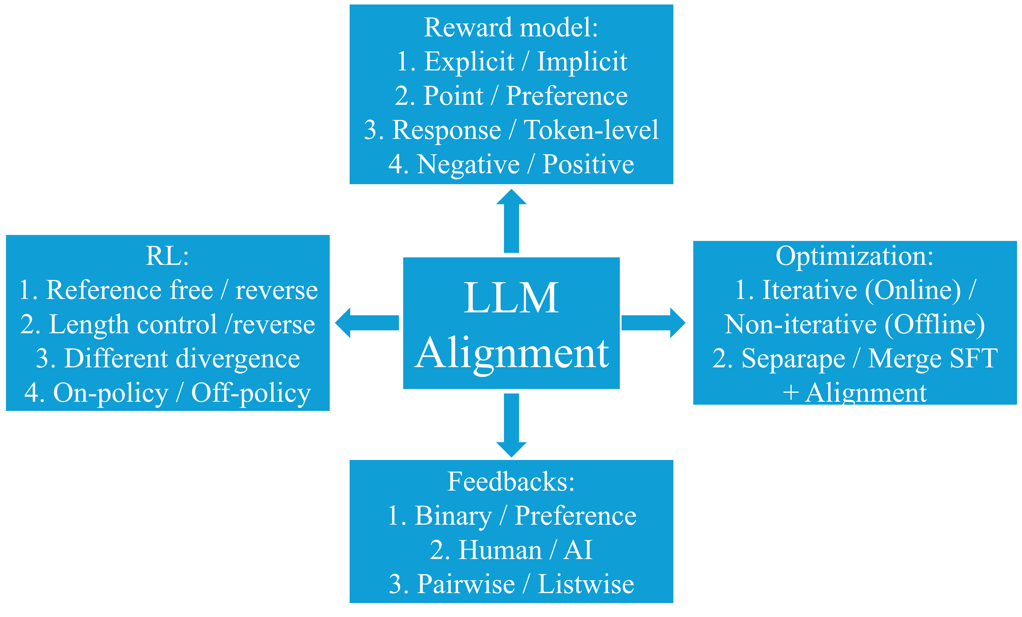
Figure 1: The 13 categorical directions for xPO to align an LLM with human preference

In this paper, we have structured our review into four main topics: 1. Reward Model; 2. Feedback; 3. Reinforcement Learning (RL); and 4. Optimization. Each topic was further divided into subtopics as shown in Figure. 1. For the Reward Model, the subtopics were: 1. Explicit Reward Model vs. Implicit Reward Model; 2. Pointwise Reward Model vs. Preference Model; 3. Response-Level Reward vs. Token-Level Reward and 4. Negative Preference Optimization. Regarding Feedback, the subtopics included: 1. Preference Feedback vs. Binary Feedback; 2. Pairwise Feedback vs. Listwise Feedback; and 3. Human Feedback vs. AI Feedback. In the RL section, the subtopics were: 1. Reference-Based RL vs. Reference-Free RL; 2. Length-Control RL; 3. Different Divergences in RL and 4. On-Policy RL vs. Off-Policy RL. For Optimization, the subtopics were: 1. Online/Iterative Preference Optimization vs. Offline/Non-iterative Preference Optimization; and 3. Separating SFT and Alignment vs. Merging SFT and Alignment. Table LABEL:Table:_Comparison_all_papers_across_13_metrics provided an analysis of all the papers reviewed in detail using these 13 evaluation metrics.

Papers	RM1	RM2	RM3	RM4	F1	F2	F3	RL1	RL2	RL3	RL4	O1	O2
InstructGPT [2]	Explicit	Point	Response	Positive	Preference	Human	Pair	Reference	Uncontrol	KL	On	Offline	Separate
RLHF: Anthropic [3]	Explicit	Point	Response	Positive	Preference	Human	Pair	Reference	Uncontrol	KL	Off	Hybrid	Separate
Online RLHF/PPO [7]	Explicit	Point	Response	Positive	Preference	Human	Pair	Reference	Uncontrol	KL	Off	Online	Separate
Iterative RLHF/PPO [8]	Explicit	Point	Response	Positive	Preference	Human	Pair	Reference	Uncontrol	KL	Off	Online	Separate
RLAIF-Anthropic [9]	Explicit	Point	Response	Positive	Preference	AI	Pair	Reference	Uncontrol	KL	On	Offline	Separate
RLAIF-Google [10]	Explicit	Point	Response	Positive	Preference	AI	Pair	Reference	Uncontrol	KL	Off	Offline	Separate
SLiC-HF [11]	-	-	-	-	Preference	Human	Pair	Free	Uncontrol	KL	Hybrid	Offline	Separate
DPO [12]	Implicit	Point	Response	Positive	Preference	Human	Pair	Reference	Uncontrol	KL	Off	Offline	Separate
DPOP [13]	Implicit	Point	Response	Positive	Preference	Human	Pair	Reference	Uncontrol	KL	Off	Offline	Separate
$\beta$DPO [14]	Implicit	Point	Response	Positive	Preference	Human	Pair	Reference	Uncontrol	KL	Off	Offline	Separate
IPO [15]	Implicit	Preference	Response	Positive	Preference	Human	Pair	Reference	Uncontrol	KL	Off	Offline	Separate
SDPO [16]	Implicit	Point	Response	Positive	Preference	Human	Pair	Reference	Uncontrol	KL	Off	Offline	Separate
DPO: from r to Q [17]	Implicit	Point	Token	Positive	Preference	Human	Pair	Reference	Uncontrol	KL	Off	Offline	Separate
TDPO [18]	Implicit	Point	Token	Positive	Preference	Human	Pair	Reference	Uncontrol	KL	Off	Offline	Separate
Self-rewarding language model [19]	Implicit	Point	Response	Positive	Preference	AI	Pair	Reference	Uncontrol	KL	Off	Online	Separate
CRINGE [20]	Implicit	Point	Response	Positive	Preference	AI	Pair	Reference	Uncontrol	KL	Off	Online	Separate
KTO [21]	Implicit	Point	Response	Positive	Binary	Human	-	Reference	Uncontrol	KL	Off	Offline	Separate
DRO [22]	-	-	-	-	Binary	Human	-	Reference	Uncontrol	KL	Off	Offline	Separate
ORPO [23]	-	-	-	-	Preference	Human	Pair	Free	Uncontrol	-	Off	Offline	Merge
PAFT [24]	Implicit	Point	Response	Positive	Preference	Human	Pair	Reference	Uncontrol	KL	Off	Offline	Merge
R-DPO [25]	Implicit	Point	Response	Positive	Preference	Human	Pair	Reference	Control	KL	Off	Offline	Merge
SIMPO [26]	-	-	-	-	Preference	Human	Pair	Free	Control	-	Off	Offline	Separate
RLOO [27]	Explicit	Point	Response	Positive	Preference	Human	Pair	Free	Uncontrol	KL	On	Offline	Separate
LiPO [28]	Implicit	Point	Response	Positive	Preference	Human	List	Reference	Uncontrol	KL	Off	Offline	Separate
RRHF [29]	-	-	-	-	Preference	Human	List	Free	Uncontrol	-	Off	Offline	Merge
PRO [30]	Explicit	Point	Response	Positive	Preference	Human	List	Free	Uncontrol	-	Off	Offline	Merge
Negating Negatives [31]	Implicit	Point	Response	Negative	-	Human	-	Reference	Uncontrol	KL	On	Offline	Separate
Negative Preference Optimization [32]	Implicit	Point	Response	Negative	-	Human	-	Reference	Uncontrol	KL	Off	Offline	Separate
CPO [33]	Implicit	Point	Response	Negative	-	Human	-	Reference	Uncontrol	KL	Off	Offline	Merge
Nash Learning from Human Feedback [34]	-	Preference	Response	Positive	Preference	Human	Pair	Reference	Uncontrol	KL	On	Offline	Separate
SPPO [35]	-	Preference	Response	Positive	Preference	Human	Pair	Reference	Uncontrol	KL	On	Offline	Separate
DNO [36]	-	Preference	Response	Positive	Preference	Human	Pair	Reference	Uncontrol	KL	Hybrid	Offline	Separate
Beyond Reverse KL Divergence [37]	Implicit	Point	Response	Positive	Preference	Human	Pair	Reference	Uncontrol	Multiple	Off	Offline	Separate

Table 1: A comparison summary across all papers in the following 13 metrics: 1. RM1: Explicit or Implicit Reward Model; 2. RM2: Point Reward or Preference Probability Model; 3. RM3: Response or Token-level Reward; 4. RM4: Positive or Negative Reward Model; 5. F1: Preference or Binary Feedback; 6. F2: Human or AI Feedback; 7. F3: Pair or List Feedback; 8. RL1: Reference Model or Reference Model Free RL; 9. RL2: Length Control or Length Uncontrol RL; 10. RL3: KL Divergence or Other Divergence RL; 11. RL4: On-policy RL or off-policy RL; 12. O1: Online/Iterative Optimization or Offline/Non-iterative Optimization; 13. O2: Merge or Separate: SFT and Alignment

2 Categorical Outline

This section provided a concise introduction to the key elements of LLM alignment, enabling readers to grasp the essential terms and various existing research directions. It includes primarily four directions: 1. reward model, 2. feedback, 3. RL policy and 4. optimization.

2.1 Reward Model

The reward model was a fine-tuned LLM that assigned scores based on the prompt and generated response. In this subsection, we would discuss: 1. utilizing explicit or implicit reward models, 2. employing pointwise reward or preference models, and 3. using token-level or response-level reward models and 4. training reward model with solely negative preference. A plot of these different reward models could be found in Figure 2.

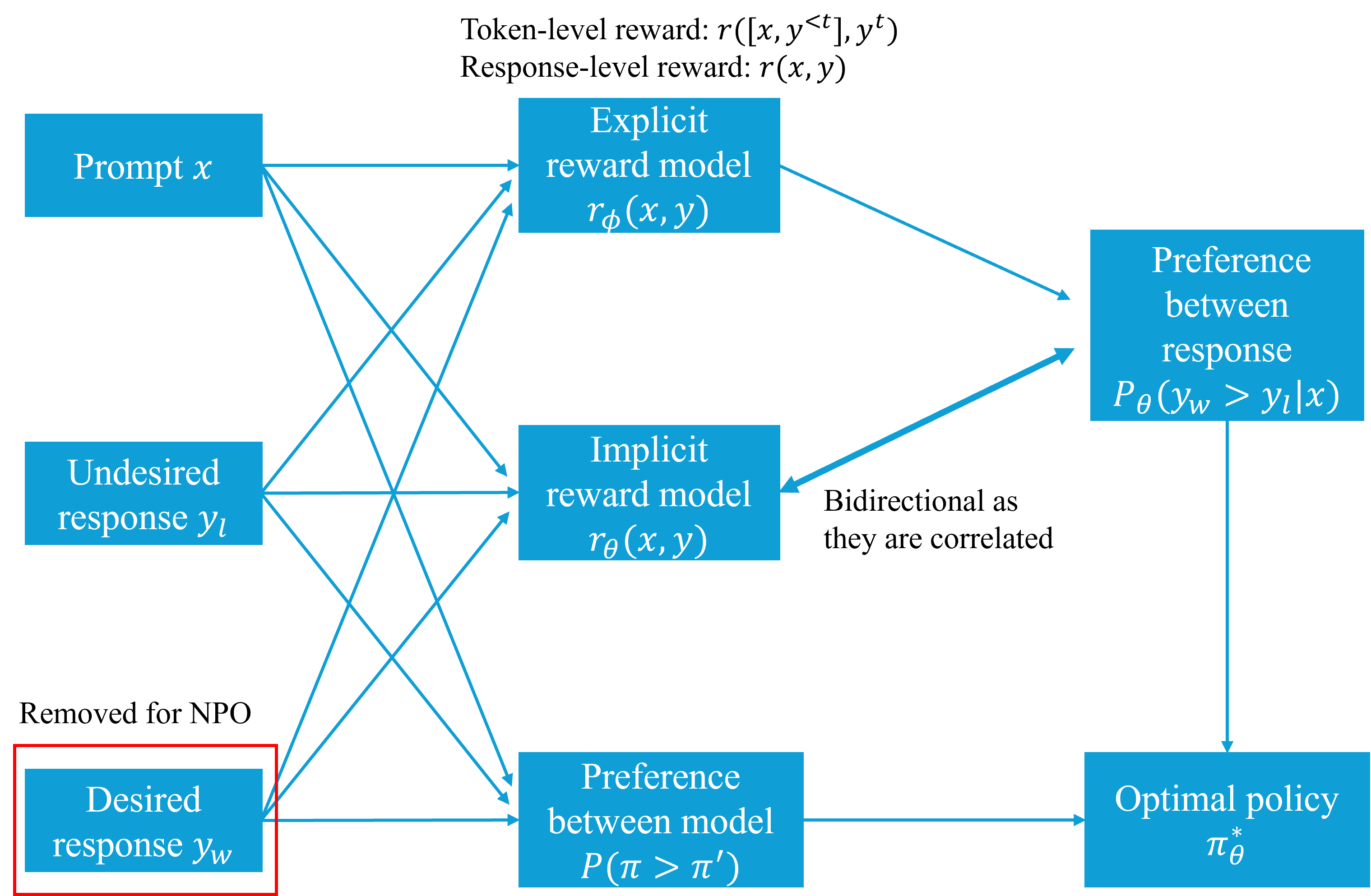
Figure 2: The four subtopics of reward model

2.1.1 Explicit Reward Model vs. Implicit Reward Model

In RLHF, researchers collected a large dataset composed of triplets, including a prompt $x$, a desired response $y_{w}$, and an undesired response $y_{l}$. Based on this collected preference dataset, explicit reward models, represented as $r_{\phi}(x,y)$ were derived by fine-tuning on pretrained LLMs to assign rewards for each prompt and response. This reward model was then used in a RL setting to align the LLM policy. Conversely, implicit reward models, represented as $r_{\theta}(x,y)$, bypassed the process of training an explicit reward model. For example, in DPO, a mapping was established between the optimal reward model and the optimal policy in RL, allowing the LLM to be aligned without directly deriving the reward model.

2.1.2 Pointwise Reward Model vs. Preferencewise Model

The original work in RLHF derived a pointwise reward model, which returned a reward score, i.e., $r(x,y)$ given the prompt $x$ and response $y$. Given two pointwise reward scores from the prompt, a desired response, and an undesired response $r(x,y_{w})$ and $r(x,y_{l})$, the probability of the desired response being preferred over the undesired response $P(y_{w}>y_{l}|x)=\sigma(r(x,y_{w})-r(x,y_{l}))$ could be obtained based on the Bradley–Terry (BT) model [38]. However, this methodology was inferior as it could not directly obtain pairwise preferences and could not accommodate inconsistencies in human labeling. To address this issue, Nash learning was proposed to directly model $P(\pi>\pi^{\prime})=\mathbb{E}_{x\sim\rho}\mathbb{E}_{y\sim\pi(y|x),y^{\prime}\sim\pi^{\prime}(y|x)}\left[P(y>y^{\prime}|x)\right]$.

2.1.3 Response-Level Reward vs. Token-Level Reward

In the original dataset collected in triplets, i.e., $\{x,y_{w},y_{l}\}$, the reward was given per response. Thus, in RLHF and DPO, the rewards were built at the response level. However, in the Markov decision process [39], rewards were given after each action, resulting in a change of state. To achieve alignment after each action, token-level reward models were introduced.

2.1.4 Negative Preference Optimization

In the RLHF dataset, human labeled both desired and undesired responses. Recently, with advancements in LLM capabilities, some researchers have posited that LLMs could generate desired responses of even higher quality than those produced by human labelers. Consequently, they opted to use only the prompts and undesired responses from the collected dataset, generating the desired responses using LLMs.

2.2 Feedback

Feedback encompassed both preferences and binary responses from humans or AI, either in pairs or lists. In this subsection, we would discuss three key distinctions: 1. preference feedback vs. binary feedback; 2. pairwise feedback vs. listwise feedback; and 3. human feedback vs. AI feedback. A plot of these feedback could be found in Figure 3.

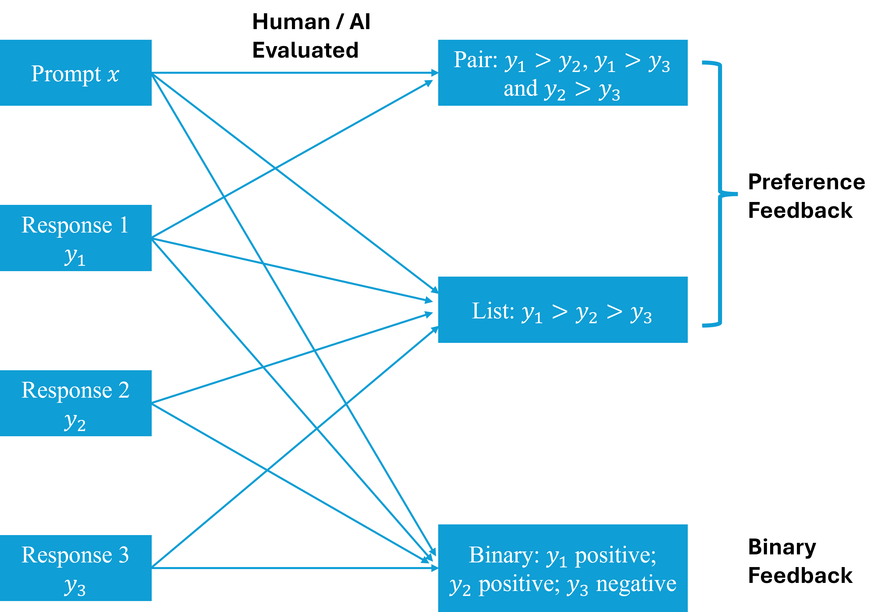
Figure 3: The four subtopics of feedback

2.2.1 Preference Feedback vs. Binary Feedback

In the RLHF paper, preference feedback, i.e., $y_{w}>y_{l}$, was collected. However, subsequent works such as KTO and DRO suggested that preference feedback was more challenging to gather, and it would be advantageous to collect binary feedback instead. Binary feedback referred to simple "thumbs up" (positive), i.e., $y^{+}$ or "thumbs down" (negative), i.e., $y^{-}$ responses.

2.2.2 Pairwise Feedback vs. Listwise Feedback

In RLHF, listwise feedback was collected. This approach involved gathering $K$ different responses $y_{1},y_{2},\ldots,y_{K}$ for a given prompt $x$ to expedite the labeling process. However, these listwise responses were then treated as $C_{K}^{2}$ pairwise responses. However, subsequent work, such as LiPO, proposed that it is more advantageous to treat listwise preferences as a ranking problem instead of viewing them as multiple pairwise preferences.

2.2.3 Human Feedback vs. AI Feedback

In RLHF, feedback was collected from humans who were asked to provide preferences given multiple responses to the same prompt. However, this process has proven to be tedious and expensive. With the latest developments in LLMs, it has become possible to collect AI feedback to align LLMs.

2.3 Reinforcement Learning (RL)

The objective of RL was formulated as $\pi^{*}_{\theta}(y|x)=\max_{\pi_{\theta}}\mathbb{E}_{x\sim D}\left[\mathbb{E}_{y\sim\pi_{\theta}(y|x)}r(x,y)-\beta D_{\text{KL}}(\pi_{\theta}(y|x)||\pi_{\text{ref}}(y|x))\right]=\max_{\pi_{\theta}}\mathbb{E}_{x\sim D,y\sim\pi_{\theta}(y|x)}\left[r(x,y)-\beta\log\frac{\pi_{\theta}(y|x)}{\pi_{\text{ref}}(y|x)}\right]$. This objective encompassed two primary goals: 1) maximizing the rewards of responses, and 2) minimizing the deviation of the aligned policy model $\pi_{\theta}(y|x)$ from the initial reference (SFT) model $\pi_{\text{ref}}(y|x)$. The discussion on RL was divided into four subtopics: 1) Reference-Based RL vs. Reference-Free RL, 2) Length-Control RL, 3) Different Divergences in RL and 4) On-policy RL vs. Off-policy RL.

2.3.1 Reference-Based RL vs. Reference-Free RL

A key aim of the RL objective in RLHF was to minimize the distance between the current policy, i.e., $\pi_{\theta}$ and the reference policy, i.e., $\pi_{\text{ref}}$. Consequently, most methodologies have focused on reference-based approaches. However, incorporating a reference policy introduced a significant memory burden. To address this issue, various methods have been proposed to avoid the reference policy. For instance, SimPO proposed a different objective that avoided the need for a reference policy altogether.

2.3.2 Length-Control RL

When using LLMs as evaluators, it has been observed that they tended to favor verbose responses, even when no additional information was provided [40]. This bias could affect the alignment of the LLM. In addition, the verbosity of LLM responses might increase the time required for humans to read and understand. The original RL objective did not account for this issue, but subsequent works such as R-DPO and SimPO incorporated considerations for length control, where $|y|$ represented the length of the output response.

2.3.3 Different Divergences in RL

In RLHF, reverse Kullback-Leibler (KL) divergence, i.e., $D_{\text{KL}}$ was commonly used to measure the distance between the current policy $\pi_{\theta}(y|x)$ and the reference policy $\pi_{\text{ref}}(y|x)$. However, KL divergence has been found to reduce the diversity of responses. To address this, research has been conducted to explore the effects of different divergence measures, i.e., $D_{f}$. More details could be found in section 3.12.

2.3.4 On-policy or Off-policy Learning

In RL, responses could be generated during training using a method called on-policy learning. The main advantage of on-policy learning was that it sampled responses from the latest version of the policy. In contrast, off-policy methods relied on responses generated earlier. Although off-policy methods could save time by avoiding the need to generate new responses during training, they had the drawback of using responses that might not align with the current policy.

2.4 Optimization

The alignment process of LLMs involved optimization. This section would discuss two key subtopics: 1. Iterative/Online Preference Optimization vs. Non-Iterative/Offline Preference Optimization; 2. Separating SFT and Alignment vs. Merging SFT and Alignment. The plot of these two subtopics on optimization could be found in Figure 4.

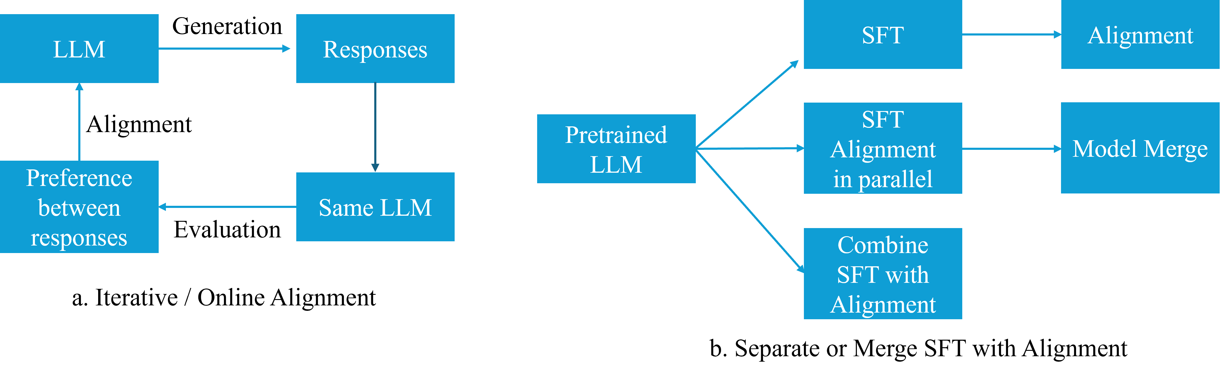
Figure 4: The two subtopics of optimization

2.4.1 Iterative/Online Preference Optimization vs. Non-Iterative/Offline Preference Optimization

When only utilizing a collected dataset for alignment, the process was referred to as non-iterative/offline preference optimization. In contrast, iterative/online preference optimization became feasible when 1. Human labeled new data or 2. LLMs assumed dual roles—both generating responses and evaluating them.

2.4.2 Separating SFT and Alignment vs. Merging SFT and Alignment

In RLHF, SFT and alignment were traditionally applied in a sequential separating manner, which could be tedious and prone to catastrophic forgetting. To address this issue, some research, such as ORPO, have proposed integrating SFT with alignment into a single process to streamline fine-tuning. Additionally, PAFT suggested fine-tuning LLMs on SFT and alignment simultaneously, then merging the results.

3 Individual Paper Reviews in Detail

In this section, we review each paper individually, offering readers a summary of the major innovations presented, so they may not need to read the papers themselves.

3.1 RLHF/PPO

LLMs were pretrained on extensive corpora sourced from various origins, which inherently could not ensure the quality of the datasets. Furthermore, the primary objective of LLMs was to predict the next token, a goal that diverged from the aim of "following the user’s instructions helpfully and safely" [2]. Consequently, LLMs could produce outputs that were untruthful, toxic, or otherwise unhelpful to users. In essence, these models were not aligned with the users’ intents. The principal aim of RLHF/PPO was to align language models with user intent across a broad spectrum of tasks by fine-tuning them using human feedback. Various studies have been conducted on this subject.

3.1.1 InstructGPT

The authors from OpenAI introduced InstructGPT, which served as a foundation for training models like ChatGPT and GPT-4 [4]. The inclusion of human preferences addressed the challenge of evaluating responses generated by LLMs. Traditional evaluation metrics such as BLEU [41], ROUGE [42], and BERTScore [43] were often utilized to evaluate LLM but they could not guarantee consistence with human preference. To tackle this issue, researchers directly incorporated human preferences into LLMs to enhance their performances. This process typically involved two main steps: reward model learning and RL policy training.

In the reward model learning phase, an explicit pointwise reward function was trained using prompts and pairwise responses, specifically one desired and one undesired response $y_{w}$ and $y_{l}$ labeled by humans through the BT model [38], as illustrated in Eq. 1.

$$L_{\text{RM}}(r_{\phi})=-\frac{1}{C_{K}^{2}}\mathbb{E}_{(x,y_{w},y_{l})\sim D}\left[\log\left(\sigma\left(r_{\phi}(x,y_{w})-r_{\phi}(x,y_{l})\right)\right)\right]$$ (1)

During the collection of reward model preference datasets, the authors presented labelers with a range of $K=4$ to $K=9$ responses to rank. This method produced $C_{K}^{2}$ comparisons for each prompt shown to a labeler. The notation $(x,y_{w},y_{l})\sim D$ was used to denote the sampling of the prompt, the desired response, and the undesired response from the collected dataset. The explicit pointwise reward model was denoted as $r_{\phi}(x,y)$.

Subsequently, the RL policy training phase commenced, wherein the LLM and the pretrained reward model functioned as the agent and the environment, respectively, within the RL framework. The objective function for RL policy training was detailed in Eq. 2 where $\pi^{*}_{\theta}$ referred to the optimal policy.

$$\pi^{*}_{\theta}(y|x)=\max_{\pi_{\theta}}\mathbb{E}_{x\sim D}\left[\mathbb{E}_{y\sim\pi_{\theta}(y|x)}r_{\phi}(x,y)-\beta D_{\text{KL}}(\pi_{\theta}(y|x)||\pi_{\text{ref}}(y|x))\right]+\gamma\mathbb{E}_{x\sim D_{\text{pretrain}}}\left[\log(\pi_{\theta}(x))\right]$$ (2)

The objective function in RL served three primary goals: 1. maximizing rewards represented by $r_{\phi}(x,y)$. 2. minimizing the divergence between the current RL policy and the initial reference (SFT) policy quantified by $D_{\text{KL}}(\pi_{\theta}(y|x)||\pi_{\text{ref}}(y|x))$. 3. avoiding the "alignment tax" in the RLHF process expressed as $\log(\pi_{\theta}(x))$ on pretaining datasets. The term "alignment tax" referred to the degradation in the performance of the LLM on downstream tasks following alignment. The parameter $\beta$ was used to control the weight of the KL divergence, with the authors suggesting that the optimal value lied between 0.01 and 0.02. When $\gamma=0$, the loss function corresponded to the standard RLHF loss. When $\gamma\neq 0$, the modified loss function was termed PPO-ptx, which addressed performance degradation on public NLP datasets.

For training InstructGPT, three datasets were utilized: 1. SFT dataset: contained labeler demonstrations used to train the SFT models. 2. RM dataset: comprised labeler rankings of model outputs, which were used to train RMs. 3. PPO dataset: composed of prompts used as input for RLHF fine-tuning. Despite the complexity of the task, the inter-annotator agreement rates were notably high. Training labelers agreed with each other 72.6 ± 1.5% of the time, while held-out labelers showed an agreement rate of 77.3 ± 1.3%.

The authors trained a single 6B reward model to be utilized for training RLHF/PPO policy models of varying sizes. They also experimented with larger 175B reward models [44]. Although larger RMs exhibited lower validation loss, their training processes were unstable and significantly increased the computational requirements for RLHF/PPO. The authors claimed that since the same input prompt generated $K$ outputs, these outputs were correlated. A straightforward method to address this was to shuffle and train them randomly. However, this approach led to overfitting. To mitigate this issue, the authors trained all $C_{k}^{2}$ comparisons as a batch, which improved the overfitting problem. One limitation of this method was that it did not account for the relative scores between responses; that was, pair responses with similar scores or those with very large score differences were treated the same. Subsequent works have considered this problem [28].

The trained InstructGPT was evaluated from three perspectives: Helpful, Honest, and Harms. "Helpful" meant that the model should follow instructions and infer intention from a few-shot prompt or another interpretable pattern, and it was evaluated by human labelers. "Honest" referred to two metrics: (1) evaluating the model’s tendency to fabricate information on closed-domain tasks and (2) performance on the TruthfulQA benchmark [45]. "Harms" involved labelers evaluating whether an output was inappropriate in the context of a customer assistant. From human evaluation, the authors claimed that "outputs from the 1.3B parameter InstructGPT model were preferred to outputs from the 175B GPT-3, despite having 100x fewer parameters." Notably, InstructGPT showed improvements in truthfulness and toxicity tasks over GPT-3, which was crucial for alignment. PPO-ptx has also demonstrated reduced performance decrement on various NLP benchmarks.

3.1.2 RLHF - Anthropic

Anthropic has conducted research on the same topic [3]. To facilitate a clear comparison, we would emphasize the distinctions between the two studies. To start, OpenAI selected labelers by filtering workers based on agreement rates or other direct measures of label quality, achieving approximately a 76% inter-labeler agreement rate. In contrast, Anthropic hypothesized that crowdworkers who demonstrated strong writing skills and engaged the AI in more stimulating discussions would likely possess better judgment regarding which AI responses were most "helpful" and "harmless". However, they observed a low average agreement rate (around 63%) between Anthropic researchers and their crowdworkers. This comparison underscored the importance of implementing filtering tasks to identify high-quality labelers.

Furthermore, the data collection methodology varied significantly. The authors focused on two primary metrics: "harmless" and "helpful", with "helpful" encompassing "honest". These metrics guided the creation of two distinct datasets. For the "helpful" dataset, crowdworkers employed LLMs to assist in generating responses. Conversely, the "harmless" dataset involved a different approach. Here, crowdworkers engaged in adversarial probing or "red-teaming" of the language models to elicit harmful responses, such as inducing the AI to use toxic language. The metrics "helpful" and "harmless" often stood in opposition to each other. The authors found that integrating these datasets for preference modeling enhanced performance on both metrics, particularly when the preference models were sufficiently large. Consistent with OpenAI’s approach, preference-strength information was disregarded, and all preference pairs were treated equally.

OpenAI has discovered that RLHF helped with alignment but could degrade performance on certain NLP benchmarks, a phenomenon referred to as the "alignment tax". Its InstructGPT model had a size of 1.3B parameters. In contrast, researchers at Anthropic evaluated seven different models with size ranging from 13M to 52B, following a geometric progression with increments of approximately $4\times$. They concluded that alignment imposed a tax on smaller models, whereas it provided a benefit for larger models, particularly those with 13B and 52B parameters. Given this alignment advantage, the authors also experimented with incorporating coding techniques datasets to enhance the capabilities of LLMs. In OpenAI’s RLHF approach, they introduced both PPO and PPO-ptx, with PPO-ptx designed to mitigate the alignment tax on NLP benchmarks. Anthropic’s RLHF findings indicated that PPO alone could achieve an alignment bonus for larger models on NLP downstream tasks. They also identified the optimal parameter for KL divergence in RL policy training as $\beta=0.001$.

In the process of training the reward model, the authors identified a near log-linear relationship between reward model accuracy and the sizes of both the model and the dataset. Larger reward models demonstrated greater robustness compared to smaller ones during the RL policy training. Then, the authors divided the preference data into two halves: a training half and a testing half. They trained separate reward models on each half, referred to as the train RM and the test RM, respectively. The RLHF policies were trained using the train RM and evaluated with the test RM. During evaluation, it was observed that "the two scores by train and test RMs are in close agreement during early stages of training, but eventually diverge, with the test RM providing a lower score." This resulted in the conclusion that the reward model had overfitted to the training data: "the reward model is less robust and more easily exploited at higher rewards". However, when larger RMs were utilized, this overfitting issue was not significantly transferred to the RLHF policy. Additionally, during the RL policy training, a linear trend was discovered between reward and $D_{\text{KL}}(\pi_{\theta}||\pi_{\text{ref}})$. Then, the authors also employed out-of-distribution (OOD) techniques to detect and reject poor requests. Finally, they explored an online training mode where both the reward model and RL policy could be updated weekly with new human preference data obtained through interactions with crowdworkers. These findings were not reported in the OpenAI InstructGPT paper.

3.1.3 Online / Iterative RLHF

RLHF techniques for aligning LLMs with human preferences have traditionally been offline methods. In the paradigm of RLHF, a static dataset, i.e., a preference dataset of the form $D=\{(x,y_{w},y_{l})\}$, where $y_{w}$ was a response preferred over $y_{l}$ given a prompt $x$ was prepared to train a reward function $r_{\phi}(x,y)$ based on the BT model [38], and then the LLM policy was optimized by leveraging the RLHF/PPO algorithm to optimize a constrained version of the reward model $\left(r_{\phi}(x,y)-\beta\log\left(\frac{\pi_{\theta}(y|x)}{\pi_{\text{ref}}(y|x)}\right)\right)$, which controlled the cumulative rewards and the divergence of the policy $\pi_{\theta}(y|x)$ from the initial SFT policy $\pi_{\text{ref}}(y|x)$. In alternative direct preference optimization methods like DPO, which skipped reward function modeling, the static dataset was leveraged to approximate optimal policy: $\log\left\{\sigma\left[\beta\log\left(\frac{\pi_{\theta}(y_{w}|x)}{\pi_{\text{ref}}(y_{w}|x)}\right)-\beta\log\left(\frac{\pi_{\theta}(y_{l}|x)}{\pi_{\text{ref}}(y_{l}|x)}\right)\right]\right\}$ and more details could be found in Section 3.3.3.

The drawback of training RLHF/PPO using offline dataset lied in the responses ($y_{w},y_{l}$) in the static dataset itself came from other LLM policies, and the preferences $y_{w}>y_{l}$ came from some oracle like human or other AI agent. Critically, the training process of reward model could not further query the preference oracle as the preference data has been fixed. However, the finite dataset $D$ might lead to over-optimization of reward on in-distribution data, since the finite dataset was a small sample of the universe of prompt-response pairs. The resulting policy model often performed poorly when faced with out-of-distribution data [8].

To deal with out-of-distribution data, the policy needed to be continuously fine-tuned, by generating pairs of response for new prompts from the intermediate policy, getting preference feedback from the oracle and feeding it back to the policy, i.e., iterative/online learning. In practise, the iterative learning was divided into two parts [7]:

1. Preference oracle training: Since it was difficult/infeasible to get expert human preference feedback continuously on new data, a preference model, i.e., a different LLM was trained on large and diverse set of offline preference data. This model, on being given a new (a prompt, pair of responses), could score each (a prompt, a response), with preferred response getting higher score.

2. Iterative policy optimization: First, a base policy model was instruction fine-tuned from a pre-trained LLM ($\pi_{\text{ref}}$). Then, the policy was continuously fine-tuned, using an exploitation and exploration framework. In the exploration phase, the current, main policy produced a response for each prompt, and an enhancer policy produced another response for the same prompt, with the preference label for the responses obtained from the preference oracle from previous step. The job of the enhancer policy was to probe in the space where there was higher uncertainty in response relative to the main policy. In the exploitation phase, the current, main policy was updated using RLHF/PPO or DPO techniques on the new preference data. Lastly, the process was then repeated to further improve the quality of the main LLM policy. The enhancer policy, in practice, could be obtained through heuristics. Popular heuristics were adjusting temperature of main policy to create enhancer policy, or rejection sampling, where main policy produced multiple responses, which were ranked by preference oracle, and best and worst response were considered to be obtained from main and enhancer policy.

Significant empirical evaluation in [7] indicated improvement in result of of policy trained through online RL, over offline RL.

3.2 RLAIF

The Reinforcement Learning from AI Feedback (RLAIF) framework was developed to mitigate the substantial expenses involved in acquiring human preference datasets. Additionally, as the capabilities of LLMs continued to advance, this approach allowed for the collection of more accurate AI preference datasets, thereby enhancing the alignment of LLMs.

3.2.1 RLAIF-Anthropic

Building on the foundational work of RLHF, a novel approach termed RLAIF was introduced [9]. This methodology encompassed two primary stages: 1. Supervised learning through Critiques and Revisions guided by a "constitution" and 2. RLAIF.

In the initial stage, the authors employed the chain of thought (CoT) framework [46] to identify potential harms in harmless data using specific principle-based instructions, which they referred to as "Constitutional AI (CAI)." For CAI, a LLM served as a critic, providing revisions. The findings indicated that self-supervised critiques and revisions could surpass human performance. During this process, the authors noted a decrease in helpfulness scores, while the combined scores for harmlessness and helpfulness (HH) improved. Additionally, increasing the number of revisions proved advantageous, as it led to the identification and correction of more harmful responses. Importantly, the critique process was found to be crucial, with the critique-revision approach outperforming the revision process alone. Following the critique and revision phase, SFT was applied to the LLM using the revised responses from critique-revision stage.

In the second stage, the authors substituted RLHF with RLAIF. During the initial stage, human annotators labeled the helpfulness data, whereas AI systems labeled the harmlessness data, as previously mentioned. Furthermore, distinct principles for constitution and CoT reasoning were employed to align the LLM, aiming to minimize harm while preserving helpfulness.

This study demonstrated the feasibility of self supervised AI alignment by utilizing AI to collect preference data. However, it was limited to harmlessness rather than helpfulness, given that the task of ensuring harmlessness was considerably simpler compared to that of ensuring helpfulness.

3.2.2 RLAIF-Google

Building on the work of RLAIF by Anthropic, the authors contended that prior research have not directly compared the effectiveness of human versus AI feedback, warranting further investigation [10]. During the AI feedback collection process, a structured prompt was created, consisting of: 1. Preamble, 2. Few-shot exemplars (optional), 3. Sample to annotate, and 4. Ending. A two-step evaluation was performed to generate AI feedback: initially, all four components of the instruction, combined with CoT, were used to generate responses from the LLM. In the subsequent stage, the LLM’s response, appended with an ending like "preferred summary=", was sent back to the LLM to generate preference probabilities such as "summary 1=0.6, summary 2=0.4". To mitigate positional bias, the sequences of the two responses were alternated, and the average scores were calculated.

In the RLAIF process, two strategies were employed: 1. "Distilled RLAIF", which adhered to the traditional RLHF approach by using preference to train a Reward Model, which was then used to train the LLM policy, and 2. "Direct RLAIF", which leveraged LLM feedback by prompting it to output evaluation scores directly as signals for policy training in RL.

Lastly, during the evaluation process, three key metrics were employed: 1. AI-labeler alignment: the degree of agreement between AI and human labelers, 2. win rate: the likelihood of a response being selected by human labelers when compared between two candidates, and 3. harmless rate: the percentage of responses deemed harmless by human evaluators.

Experiments were conducted on three datasets: 1. Reddit TL;DR (summary) [47], 2. OpenAI’s Human Preferences (helpful) [47], and 3. Anthropic Helpful and Harmless (HH; harmless) Human Preferences [3]. PaLM 2 was utilized as the LLM for alignment [48].

The authors made a couple of observations on the summarization task. They observed that the RLHF policy sometimes hallucinated when the RLAIF policy did not and RLAIF sometimes produced less coherent summaries as compared to RLHF. They mentioned that more systemaic analysis was required to understand if these patterns existed at scale.

Three main conclusions were drawn. Firstly, RLAIF achieved comparable performance to RLHF in summarization and helpful dialogue generation tasks, but outperformed RLHF in the harmless task. Secondly, RLAIF demonstrated the ability to enhance a SFT policy even when the LLM labeler was of the same size as the policy. Lastly, "Direct RLHF" surpassed "Distilled RLHF" in terms of alignment.

3.3 Direct Human Preference Optimization

Traditional RLHF methods typically involved optimizing a reward function derived from human preferences. While effective, this approach could introduce challenges such as increased computational complexity and a bias-variance trade-off in estimating and optimizing rewards [49]. Recent research has explored alternative methods that aimed to optimize LLM policies directly based on human preferences, without necessarily relying on a scalar reward signal.

These approaches sought to simplify the alignment process, reduce computational overhead, and potentially achieve more robust optimization by working more directly with preference data. By framing the problem as one of preference optimization rather than reward estimation and maximization, these methods offered a different perspective on aligning language models with human judgments.

3.3.1 SliC-HF

This study introduced Sequence Likelihood Calibration with Human Feedback (SLiC-HF) to align LLMs with human preferences by employing a max-margin ranking loss with regularization, as shown in Eq. 3 [11].

$$L_{\text{SLiC-HF}}(\pi_{\theta})=\max\left(0,\delta-\log P_{\theta}(y_{w}|x)+\log P_{\theta}(y_{l}|x)\right)-\lambda\log P_{\theta}(y_{\text{ref}}|x)$$ (3)

Here $\delta$ served as a margin to distinguish desired responses from undesired responses, and the regularization term $-\lambda\log P_{\theta}(y_{\text{ref}}|x)$ would encourage the trained model to stay close to the initial SFT policy.

The authors proposed two main variants: SLiC-HF-direct and SLiC-HF-sample-rank. SLiC-HF-direct used human preference feedback data directly to define desired response $y_{w}$ and undesired response $y_{l}$. In contrast, SLiC-HF-sample-rank generated multiple responses from the SFT model and then used a separate ranking or reward model to determine $y_{w}$ and $y_{l}$ from these generated responses. This sample-rank variant ensured that the training examples were drawn from the model’s current output distribution, potentially leading to more stable and effective learning compared to using off-policy human preference data. The authors found that SLiC-HF-sample-rank converged more robustly.

The study demonstrated that SLiC-HF could achieve comparable or superior performance to RLHF/PPO methods while using significantly less computational resources, i.e., 0.25 the memory footprint of PPO training paradigm. On the Reddit TL;DR summarization task [3], a T5-Large (770M parameters) [50] model trained with SLiC-HF outperformed a 6B parameter model trained with RLHF/PPO. This result suggested that SLiC-HF represented a promising direction for aligning LLMs with human preferences, offering a balance between performance, computational efficiency, and implementation simplicity.

3.3.2 RSO

Rejection Sampling Optimization (RSO) [51] addressed limitations in offline preference optimization methods like SLiC and DPO by addressing the distribution mismatch between the training data and the data expected from the optimal policy, using statistical rejection sampling.

The rejection sampling methodology was detailed as follows:

1. Generate $y\sim\pi_{\text{SFT}}(y|x)$ and $u\sim U[0,1]$.

2. Calculate $M=\min\{m|m\pi_{\text{SFT}}(y|x)\geq\pi_{\theta}(y|x)\}$.

3. Accept $y$ if $u<\left[\frac{\pi_{\theta}(y|x)}{M\pi_{\text{SFT}}(y|x)}\approx P_{\text{accept}}(x,y)\right]$; otherwise, reject. This ensures that only responses close to the optimal policy are selected.

In comparison, $u$ was simple to sample, while $\frac{\pi_{\theta}(y|x)}{M\pi_{\text{SFT}}(y|x)}$ was tough to obtain. To solve this problem, RSO used a trained reward model $r_{\phi}(x,y)$ to guide the sampling process. The algorithm generated candidates from the SFT policy $\pi_{\text{SFT}}(y|x)$ and accepted them based on the calculated probability $P_{\text{accept}}(x,y)$ as shown in Eq. 4 where $r_{\text{max}}$ referred the maximum reward left in the current samples sets.

$$P_{\text{accept}}(x,y)=e^{\left(\frac{r_{\phi}(x,y)-r_{\text{max}}}{\beta}\right)}$$ (4)

Here, $\beta$ controlled the selectiveness of the sampling. As $\beta\to\infty$, every response was accepted (i.e., $P_{\text{accept}}\to 1$ for all $y$), and as $\beta\to 0$, only the highest reward response was accepted.

The authors conducted experiments on the TL;DR summarization [47] and Anthropic HH dialogue datasets [3]. The T5-large model (770M) was initialized as SFT, while the T5-XXL (11B) served as the reward model [52]. Evaluation results demonstrated that RSO surpassed previous methods including SLiC and DPO across multiple metrics, including human evaluation. RSO also showed better scalability to larger models and improved cross-task generalization.

RSO offered a more principled approach to generating training data that approximated on-policy RL. Its unified framework and intelligent sampling strategy could serve as catalyst to other off-policy training methods as well.

3.3.3 DPO

RLHL/PPO necessitated an initial phase of training a reward model using a preference dataset, followed by training a RL policy with the pretrained reward model serving as the environment. This bifurcated training process demanded meticulous oversight, including significant computational resources to hold multiple models in the memory (reward, value, policy, reference); data collection for training both the reward model and the RL policy, and monitoring for overfitting. To address these challenges, Direct Preference Optimization (DPO) was introduced [12]. The objective function in PPO-based RL was shown in Eq. 5 to derive $\pi_{\theta}^{*}(y|x)$.

$$\pi^{*}_{\theta}(y|x)=\max_{\pi_{\theta}}\mathbb{E}_{x\sim D}\left[\mathbb{E}_{y\sim\pi_{\theta}(y|x)}r_{\theta}(x,y)-\beta D_{\text{KL}}\left(\pi_{\theta}(y|x)\|\pi_{\text{ref}}(y|x)\right)\right]$$ (5)

Based on the RL objective, given a reward model, i.e., $r_{\theta}(x,y)$, the optimal policy, i.e., $\pi_{\theta}(y|x)$ could be expressed as Eq. 6. $Z(x)$ represented a term dependent solely on the input, used to normalize $\pi_{\theta}(y|x)$. The initial policy before DPO was indicated by $\pi_{\text{ref}}(y|x)$. The hyperparameter $\beta$ controlled the divergence between the reference policy and the final aligned policy post-DPO.

$$\pi_{\theta}(y|x)=\frac{1}{Z(x)}\pi_{\text{ref}}(y|x)e^{\left(\frac{1}{\beta}r_{\theta}(x,y)\right)}$$ (6)

By rewriting Eq. 6, the reward model could be illustrated in term of the RL policy as illustrated in Eq. 7

$$r_{\theta}(x,y)=\beta\log\left(\frac{\pi_{\theta}(y|x)}{\pi_{\text{ref}}(y|x)}\right)+\beta\log Z(x)$$ (7)

By expressing the reward function $r_{\theta}(x,y)$ in terms of the optimal policy $\pi_{\theta}(y|x)$, we could optimize them simultaneously in the reward model training process. Lastly, the formulation of $Z(x)$ was given by: $Z(x)=\sum_{y}\pi_{\text{ref}}(y|x)e^{\left(\frac{1}{\beta}r_{\theta}(x,y)\right)}$. It was evident that $Z(x)$ depended only on $x$ as it involved summation over all possible $y$, which was computationally intractable. Due to this intractability, DPO suggested eliminating this term by subtraction, as demonstrated in Eq. 8.

$$r_{\theta}(x,y_{w})-r_{\theta}(x,y_{l})=\beta\left[\log\left(\frac{\pi_{\theta}(y_{w}|x)}{\pi_{\text{ref}}(y_{w}|x)}\right)-\log\left(\frac{\pi_{\theta}(y_{l}|x)}{\pi_{\text{ref}}(y_{l}|x)}\right)\right]$$ (8)

Lastly, by employing the BT model as illustrated in Eq. 9, the pairwise preference $P_{\theta}(y_{w}>y_{l}|x)$ was articulated in terms of the pointwise reward $r_{\theta}(x,y)$, which was defined through the optimal policy $\pi_{\theta}(y|x)$.

$$P_{\theta}(y_{w}>y_{l}|x)=\sigma(r_{\theta}(x,y_{w})-r_{\theta}(x,y_{l}))\\ =\sigma\left[\beta\log\left(\frac{\pi_{\theta}(y_{w}|x)}{\pi_{\text{ref}}(y_{w}|x)}\right)-\beta\log\left(\frac{\pi_{\theta}(y_{l}|x)}{\pi_{\text{ref}}(y_{l}|x)}\right)\right]$$ (9)

Substituting this into the cross-entropy with $P^{\prime}(y_{w}>y_{l}|x)=1$ and $P^{\prime}(y_{w}>y_{l}|x)=0$, the final loss function of DPO was derived, as shown in Eq. 10.

$$L_{\text{DPO}}(\pi_{\theta})=-\mathbb{E}_{(x,y_{w},y_{l})\sim D}\log P_{\theta}(y_{w}>y_{l}|x)=-\mathbb{E}_{(x,y_{w},y_{l})\sim D}\log\left\{\sigma\left[\beta\log\left(\frac{\pi_{\theta}(y_{w}|x)}{\pi_{\text{ref}}(y_{w}|x)}\right)-\beta\log\left(\frac{\pi_{\theta}(y_{l}|x)}{\pi_{\text{ref}}(y_{l}|x)}\right)\right]\right\}$$ (10)

The authors have also derived the gradient of DPO, as illustrated in Eq. 11. This gradient maximized the likelihood of $y_{w}$ while minimized the likelihood of $y_{l}$. Concurrently, a weighting term $\sigma(r_{\theta}(x,y_{l})-r_{\theta}(x,y_{w}))$ was introduced, which imposed a higher penalty when the difference between the rewards of $y_{w}$ and $y_{l}$ approached negative infinity. As this difference increased and approached positive infinity, the penalty gradually decreased. This penalization was logical, as a higher penalty should be applied when the rewards of $y_{l}$ were similar to or greater than those of $y_{w}$. Conversely, if the reward of $y_{w}$ significantly exceeded that of $y_{l}$, minimal modification was necessary, and it was reasonable for the gradient to be smaller.

$$\nabla_{\theta}L_{\text{DPO}}(\pi_{\theta})=-\beta\mathbb{E}_{(x,y_{w},y_{l})\sim D}[\sigma(r_{\theta}(x,y_{l})-r_{\theta}(x,y_{w}))(\nabla_{\theta}\log\pi_{\theta}(y_{w}|x)-\nabla_{\theta}\log\pi_{\theta}(y_{l}|x))]$$ (11)

The authors proposed that "two reward functions $r(x,y)$ and $r^{\prime}(x,y)$ were considered equivalent if and only if $r(x,y)-r^{\prime}(x,y)=f(x)$ for some function $f$." This established the equivalence of $r_{\theta}(x,y)=\beta\log\frac{\pi_{\theta}(y|x)}{\pi_{\text{ref}}(y|x)}+\beta\log Z(x)$ and $r_{\theta}(x,y)=\beta\log\frac{\pi_{\theta}(y|x)}{\pi_{\text{ref}}(y|x)}$ in deriving the same optimal policy, as the difference was solely dependent on the input $x$.

Upon training with DPO, the optimal policy could be directly obtained without the need for generating an intermediate reward function, thereby simplifying the training process of RLHF. In summary, DPO facilitated the extraction of the corresponding optimal policy in a closed form, deriving the resolution of the standard RLHF problem using only a straightforward classification loss.

Furthermore, the authors have extended the DPO loss function to handle noisy data in labeling, as demonstrated in Eq. 12, by substituting $P^{\prime}(y_{w}>y_{l}|x)=1-\epsilon$ and $P^{\prime}(y_{w}>y_{l}|x)=\epsilon$.

$$L^{\epsilon}_{\text{DPO}}(\pi_{\theta})=-\mathbb{E}_{(x,y_{w},y_{l})\sim D}\left[(1-\epsilon)\log P_{\theta}(y_{w}>y_{l}|x)+\epsilon\log(1-P_{\theta}(y_{w}>y_{l}|x))\right]$$ (12)

However, there were certain limitations associated with DPO. In the RLHF approach used by OpenAI, the reward model remained unchanged, facilitating human alignment. For further training on related tasks, only new prompts were required, with responses generated by the LLM and rewards obtained from the existing reward model. This approach offers significant advantages in flexibility and reusability. For instance, consider an user who has built an English summarization model with a corresponding reward model. To extend this to Spanish texts, they could potentially reuse the English reward model as a naive initialization for Spanish rewards. In contrast, DPO required new preference data for further optimization, which can be challenging to obtain as it necessitated meticulous human labeling. Using the same example, DPO would require collecting an entirely new set of preference data for Spanish summaries, involving multiple Spanish summaries for each text and bilingual human annotators to compare and rank them. This process is significantly more resource-intensive than generating new prompts in Spanish for the RLHF approach.

Furthermore, the loss function of DPO focused solely on maximizing the difference between desired and undesired responses. Based on this loss function, it was possible to inadvertently reduce the rewards for desired responses or increase the rewards for undesired responses. Although the authors have claimed that two reward functions were equivalent if their differences depended only on input prompts, we might still prefer the rewards for $y_{w}$ to increase and the rewards for $y_{l}$ to decrease. Suppose a model generated a response to a prompt, and the corresponding reward was relatively low. In this scenario, it became challenging to determine the quality of the response. It might turn out that the output was of high quality, though the implicit reward score was low. Under these conditions, we had to generate multiple outputs, calculate their reward scores, and select the best solution.

Recent studies have also shown that DPO is particularly sensitive to distribution shifts between the base model outputs and the preference data [53]. This sensitivity can lead to poor performance when there’s a mismatch between the training data of the base model and the preference dataset. To address this issue, iterative DPO has been proposed, where new responses are generated with the latest policy model and a critique (can be either separate reward model or same policy network in a self-rewarding setting) are used for preference labeling in each iteration. This approach can help mitigate the distribution shift problem and potentially improve DPO’s performance.

Lastly, the tests in the DPO paper were primarily conducted on simple cases, including the IMDB dataset [54] for controlled sentiment generation and Reddit dataset [47] for summarization. More complex downstream NLP tasks should be evaluated to assess the effectiveness of DPO, especially in light of the distribution shift sensitivity and the potential benefits of iterative DPO.

3.3.4 DPOP: Smaug

The DPO loss function aimed to maximize the disparity between desired and undesired responses. However, this approach could be problematic. It might lead to simultaneous increases or decreases in the rewards for both desired and undesired responses, as long as the difference between them grew. The authors theoretically demonstrated that the rewards for both types of responses could decrease concurrently [13]. This phenomenon was particularly pronounced in data with small edit (Hamming) distances. For instance, "2+2=4" and "2+3=4" had an edit distance of 1. To address the limitations of DPO in scenarios with small edit distances, the authors created three datasets: modified ARC [55], Hellaswag[56], and Metamath [57], which included more examples with small edit distances. They also introduced DPO-positive (DPOP), as defined in Eq. 13.

$$L_{\text{DPOP}}(\pi_{\theta})=-\mathbb{E}_{(x,y_{w},y_{l})\sim D}\left\{\log\left[\sigma\left(\beta\log\left(\frac{\pi_{\theta}(y_{w}|x)}{\pi_{\text{ref}}(y_{w}|x)}\right)-\beta\log\left(\frac{\pi_{\theta}(y_{l}|x)}{\pi_{\text{ref}}(y_{l}|x)}\right)\right)\right]-\lambda\max\left(0,\log\left(\frac{\pi_{\text{ref}}(y_{w}|x)}{\pi_{\theta}(y_{w}|x)}\right)\right)\right\}$$ (13)

By incorporating the term $\max\left(0,\log\left(\frac{\pi_{\text{ref}}(y_{w}|x)}{\pi_{\theta}(y_{w}|x)}\right)\right)$, we could effectively prevent the reduction in rewards for desired responses. This is because the logits of preferred generation are incentivized to improve over the reference model in addition to the standard DPO loss, and this avoids the undesirable situation described above. Utilizing this revised loss function, the authors trained and evaluated Smaug-7B, 34B, and 72B models on the Huggingface LLM leaderboard and MTBench [58]. Notably, the 70B scale models achieved state-of-the-art performance on the Huggingface LLM leaderboard when the paper was published.

3.3.5 $\beta$-DPO

While DPO has shown promise in aligning LLMs with human preferences, its performance is sensitive to the fine-tuning of its trade-off parameter $\beta$ with respect to quality of preference data. This sensitivity could be attributed to two factors: 1. The optimal value of $\beta$ changes with the quality of preference data, requiring a dynamic approach and 2. Real-world datasets often contain outliers that can distort the optimization process. To avoid this overhead, DPO with Dynamic $\beta$ [14] introduced a framework that dynamically calibrates $\beta$ at the batch level, informed by the underlying preference data.

To address these challenges, $\beta$-DPO introduced two main components:

1. Dynamic $\beta$ Calibration at Batch-Level: This approach adjusts $\beta$ for each batch based on the quality of pairwise data. The batch-level $\beta$ is calculated as:

   $$\beta_{\text{batch}}=[1+\alpha(E_{i\sim\text{batch}}[M_{i}]-M_{0})]\beta_{0}$$ (14)

   where $M_{i}$ is the individual reward discrepancy, $M_{0}$ is a threshold, and $\alpha$ is a scaling factor.

2. $\beta$-Guided Data Filtering: This mechanism mitigates the impact of outliers by filtering them out based on a probabilistic model of reward discrepancies.

Empirical evaluations on Anthropic HH [3] and Reddit TL;DR summarization [47] tasks demonstrated that $\beta$-DPO consistently outperforms standard DPO across different model sizes and sampling temperatures. For instance, on the Anthropic HH dataset, $\beta$-DPO achieved improvements exceeding 10% on models of various sizes including Pythia-410M, 1.4B, and 2.8B [59].

A critical aspect of this approach is the consideration of pairwise data quality, rized as "low gap" or "high gap". Low gap denotes cases where chosen and rejected responses are closely similar, typically indicating high-quality, informative pairs. Instead, high gap refers to pairs with larger differences, implying lower-quality data.

Experiments with Pythia-1.4B on the Anthropic HH dataset revealed a distinct trend: for low gap data, a higher $\beta$ reduces win rate, whereas for high gap data, an increased $\beta$ improves performance. This observation highlights the necessity of tailoring the $\beta$ value to the data quality, especially in the presence of outliers.

However, limitations and areas for future work include exploring $\beta$-DPO in self-play scenarios, developing more sophisticated evaluation metrics, investigating scalability to ultra-large models, and pursuing automated parameter tuning.

3.3.6 IPO

Azar et al. identified that RLHF and DPO were susceptible to overfitting, and introduced Identity Preference Optimization (IPO) as a solution to this issue [15]. The authors highlighted two key assumptions underlying RLHF: 1. "pairwise preferences can be substituted with pointwise rewards," and 2. "a reward model trained on these pointwise rewards can generalize from collected data to out-of-distribution data sampled by the policy". They argued that in DPO the second assumption could be circumvented by learning the policy directly from data without the need for an intermediate reward function, leaving the first assumption intact. Specifically, challenges might arise when substituting pairwise preferences with a pointwise reward model using the BT model. This assumption became problematic when preferences were deterministic or nearly deterministic, i.e., $P(y_{w}>y_{l})=1$. Under deterministic conditions, $r_{\theta}(x,y_{w})-r_{\theta}(x,y_{l})=\beta\left[\log\left(\frac{\pi_{\theta}(y_{w}|x)}{\pi_{\text{ref}}(y_{w}|x)}\right)-\log\left(\frac{\pi_{\theta}(y_{l}|x)}{\pi_{\text{ref}}(y_{l}|x)}\right)\right]\to+\infty$. As this value approached positive infinity, the effectiveness of the KL divergence constraint imposed by $\beta$ diminished. Consequently, the objective function shifted towards maximizing accumulated rewards, potentially leading to overfitting.

To address the issue, the authors introduced a general objective for RLHF, which avoided the transformation preference based on pointwise reward through the BT model and focused on optimizing a nonlinear function of preferences, as detailed in Eq. 15.

$$\pi^{*}_{\theta}(y|x)=\max_{\pi_{\theta}}\mathbb{E}_{x\sim\rho}\left[\mathbb{E}_{y\sim\pi_{\theta}(y|x),\,y^{\prime}\sim\pi^{\prime}_{\theta}(y|x)}\Psi(P_{\theta}(y>y^{\prime}|x))-\beta D_{\text{KL}}(\pi_{\theta}(y|x)||\pi_{\text{ref}}(y|x))\right]$$ (15)

Two policies, $y\sim\pi_{\theta}(y|x)$ and $y^{\prime}\sim\pi^{\prime}_{\theta}(y|x)$, were employed, with the primary focus on maximizing the first policy, $y\sim\pi_{\theta}(y|x)$, during the RL policy training process. Equation 15 was equivalent to DPO when $\Psi(x)=\log\left(\frac{q(x)}{1-q(x)}\right)$. The authors attributed the overfitting observed in RLHF and DPO to the nonlinear transformation of $\Psi(x)$, stating: "small increases in probabilities already close to 1 are just as incentivized as large increases in preference probabilities around 50%, which may be undesirable". To address this issue, the authors proposed setting the function as $\Psi(x)=x$, thereby removing the nonlinear transformation in the objective of RL policy training as shown in Eq. 16.

$$\pi^{*}_{\theta}(y|x)=\max_{\pi_{\theta}}\mathbb{E}_{x\sim\rho}\left[\mathbb{E}_{y\sim\pi_{\theta}(y|x),y^{\prime}\sim\pi^{\prime}_{\theta}(y|x)}P_{\theta}(y>y^{\prime}|x)-\beta D_{\text{KL}}(\pi_{\theta}(y|x)||\pi_{\text{ref}}(y|x))\right]$$ (16)

Based on the given objective function, the authors formulated a novel loss function as illustrated in Eq. 17, and it could avoid BT model to transform pointwise rewards to preference probabilities.

$$L_{\text{IPO}}(\pi_{\theta})=-\mathbb{E}_{(x,y_{w},y_{l})\sim D}\left[\log\left(\frac{\pi_{\theta}(y_{w}|x)}{\pi_{\text{ref}}(y_{w}|x)}\right)-\log\left(\frac{\pi_{\theta}(y_{l}|x)}{\pi_{\text{ref}}(y_{l}|x)}\right)-\frac{1}{2\beta}\right]^{2}$$ (17)

This newly derived loss function could be directly optimized to obtain an optimal policy, effectively mitigating the issue of overfitting. The experiment was conducted on a basic mathematical use case, demonstrating that when the penalty coefficient $\beta$ was sufficiently large, IPO successfully avoided overfitting, whereas DPO tended to overfit. However, the modified DPO by adding noise was expected to address this issue adequately. Lastly, further use cases in downstream NLP tasks were necessary to validate the advantages of the IPO method.

3.3.7 sDPO

In the context of DPO, the reference model was essential for preserving the performance of SFT and downstream tasks. The authors posited that the reference model acted as the lower bound for DPO, suggesting that an improved reference model could provide a superior lower bound for DPO training [16]. Building on this premise, stepwise DPO (sDPO) was introduced, which segmented the preference datasets and employed them incrementally. At each stage, DPO was applied, and the resulting partially aligned model became the new reference model.

Initially, SOLAR 10.7B [60] was used as the reference model. Subsequently, two datasets OpenOrca (around 12K samples) [61] and Ultrafeedback Cleaned (around 60K samples) [62] were employed in the sDPO process, with OpenOrca used in the first step and Ultrafeedback in the second. Four tasks, i.e., ARC [55], HellaSWAG [56], MMLU [63], and TruthfulQA [45], were utilized, and their scores surpassed those of DPO. In contrast, Winogrande [64] and GSM8K [65] were excluded due to their nature as generation tasks, differing from the multiple-choice tasks previously considered. However, in our perspective, this was not a compelling reason to omit these tasks. It raised the question: could sDPO negatively impact generation tasks? Further experiments were necessary to explore this issue.

The authors have demonstrated that $\gamma_{\text{ref}}(x,y_{w},y_{l})=\log\frac{\pi_{\text{ref}}(y_{w}|x)}{\pi_{\text{ref}}(y_{l}|x)}$ increased as the number of DPO steps increased. Furthermore, they have shown that initializing the target model with the updated reference model was advantageous, as it resulted in a lower initial loss function compared to using the original reference model.

Several questions arose that could further enhance this research. The current study utilized two datasets, applying stepwise alignment to each individually. Supposed only one dataset was available, would segmenting this dataset and applying DPO sequentially to each segment yield similar benefits? Additionally, even with two datasets, would it be advantageous to use the first 50% of each dataset for the initial alignment step and the remaining 50% for the subsequent alignment stage? Finally, catastrophic forgetting was a well-known issue. Would it be beneficial to mix a portion of the previous stepwise data with the new data to mitigate this problem?

3.3.8 GPO

The authors proposed a generalized preference optimization (GPO) as shown in Eq. 18 [66].

$$L_{\text{GPO}}(\pi_{\theta})=\mathbb{E}_{(x,y_{w},y_{l})\sim D}\left\{f\left[\beta\log\left(\frac{\pi_{\theta}(y_{w}|x)}{\pi_{\text{ref}}(y_{w}|x)}\right)-\beta\log\left(\frac{\pi_{\theta}(y_{l}|x)}{\pi_{\text{ref}}(y_{l}|x)}\right)\right]\right\}$$ (18)

Then, the authors applied Taylor expansion around 0 as shown in Eq. 19 supposing $r_{\theta}(x,y_{w},y_{l})=\beta\log\left(\frac{\pi_{\theta}(y_{w}|x)}{\pi_{\text{ref}}(y_{w}|x)}\right)-\beta\log\left(\frac{\pi_{\theta}(y_{l}|x)}{\pi_{\text{ref}}(y_{l}|x)}\right)$.

$$\mathbb{E}_{(x,y_{w},y_{l})\sim D}[f(r_{\theta}(x,y_{w},y_{l}))]\approx f(0)+f^{\prime}(0)\mathbb{E}_{(x,y_{w},y_{l})\sim D}[r_{\theta}(x,y_{w},y_{l})]+\frac{f^{\prime\prime}(0)}{2}\mathbb{E}_{(x,y_{w},y_{l})\sim D}[\left(r_{\theta}(x,y_{w},y_{l})\right)^{2}]$$ (19)

$f^{\prime}(0)\mathbb{E}_{(x,y_{w},y_{l})\sim D}[r_{\theta}(x,y_{w},y_{l})]$ was termed preference optimization, and its target focused on maximizing the difference between desired and undesired responses, which played similar roles to rewards. $\frac{f^{\prime\prime}(0)}{2}\mathbb{E}_{(x,y_{w},y_{l})\sim D}[\left(r_{\theta}(x,y_{w},y_{l})\right)^{2}]$ was termed as offline regularization, and its targets lied in minimizing the difference between the current policy and the reference policy, which was similar to the KL divergence.

3.4 Token-level DPO

In DPO, rewards were assigned to a prompt and response collectively. Conversely, in MDP, rewards were allocated for each individual action. The subsequent two papers delved into elucidating DPO at the token level and expanding its application to token-level analysis.

3.4.1 DPO: from r to Q

DPO was conceptualized as a bandit problem rather than a token-level MDP [39], with the entire response treated as a single arm to receive a reward. In [17], the authors demonstrated that DPO was capable of performing token-level credit assignment. In the context of a token-level MDP, it was defined as $M=(S,A,f,r,\rho_{0})$, where $S$ represented the state space, $A$ denoted the action space, $f(s|a)$ described the state transition given an action, $r$ signified the reward functions, and $\rho_{0}$ indicated the initial state distribution. The token-level MDP was formulated within the framework of the maximum entropy setting of RL, as illustrated in Eq. 20.

$$\pi^{*}_{\theta}(y|x)=\max_{\pi_{\theta}}E_{a_{t}\sim\pi_{\theta}(a_{t}|s_{t})}\left\{\sum_{t=0}^{T}\left[r_{\theta}(s_{t},a_{t})+\beta\log\left(\pi_{\text{ref}}(a_{t}|s_{t})\right)\right]+\beta H(\pi_{\theta})\middle|s_{0}\sim\rho(s_{0})\right\}$$ (20)

In the context of maximum entropy RL, the relationship between optimal Q function $Q_{\theta}(s_{t},a_{t})$ and optimal value function $V_{\theta}(s_{t})$ was elucidated in Eq. 21.

$$Q_{\theta}(s_{t},a_{t})-V_{\theta}(s_{t})=\beta\log(\pi_{\theta}(a_{t}|s_{t}))$$ (21)

Bellman equation was shown in Eq. 22.

$$Q_{\theta}(s_{t},a_{t})=r_{\theta}(s_{t},a_{t})+\beta\log(\pi_{\text{ref}}(a_{t}|s_{t}))+V_{\theta}(s_{t+1})$$ (22)

Plugging $Q_{\theta}(s_{t},a_{t})$ in Eq. 22 into Eq. 21, we could derive $r_{\theta}(s_{t},a_{t})=V_{\theta}(s_{t})-V_{\theta}(s_{t+1})+\beta\log\left(\frac{\pi_{\theta}(a_{t}|s_{t})}{\pi_{\text{ref}}(a_{t}|s_{t})}\right)$. Furthermore, by summing on both sides and $V_{\theta}(s_{T})=0$, the cumulative rewards could be re-expressed as indicated in Eq. 23.

$$\sum_{t=0}^{T-1}r_{\theta}(s_{t},a_{t})=V_{\theta}(s_{0})+\sum_{t=0}^{T-1}\beta\log\left(\frac{\pi_{\theta}(a_{t}|s_{t})}{\pi_{\text{ref}}(a_{t}|s_{t})}\right)$$ (23)

The term $V_{\theta}(s_{0})$ could be cancelled out when plugging into the BT model as shown in 24, with $N$ tokens in $y_{w}$ and $M$ tokens in $y_{l}$.

$$P_{\theta}(y_{w}>y_{l})=\sigma\left[\sum_{t=0}^{N-1}\beta\log\left(\frac{\pi_{\theta}(a^{w}_{t}|s^{w}_{t})}{\pi_{\text{ref}}(a^{w}_{t}|s^{w}_{t})}\right)-\sum_{t=0}^{M-1}\beta\log\left(\frac{\pi_{\theta}(a^{l}_{t}|s^{l}_{t})}{\pi_{\text{ref}}(a^{l}_{t}|s^{l}_{t})}\right)\right]$$ (24)

Eventually, the bandit problem, which traditionally considered the entire response as a single entity, was redefined as a token-level MDP with rewards assigned to each token generation, specifically $\beta\log\left(\frac{\pi_{\theta}(a_{t}|s_{t})}{\pi_{\text{ref}}(a_{t}|s_{t})}\right)$.

Extensive experiments have demonstrated the efficacy of DPO in token-level MDPs. Initially, the authors successfully utilized token-level rewards to identify erroneous modifications in LLM responses $y$ given prompt $x$. Then, by employing beam search with token-level rewards, the authors generated higher quality responses, with results indicating that increasing the beam size significantly enhanced response quality. Lastly, the authors proved that during maximum entropy RL, the implicit rewards for both desired and undesired responses diminished when a model fine-tuned with SFT was used as the reference model.

3.4.2 TDPO

The authors discovered that in the DPO process, the generative diversity of LLM was deteriorated and the KL divergence grew faster for less preferred responses compared with preferred responses, and they proposed token-level DPO (TDPO) to solve these problems [18]. In original DPO, reverse KL divergence was applied, while sequential forward KL divergence was applied in token-level DPO.

For the token-level DPO problem, the reward decay was set to one, i.e., no reward decay and the token-wise reward was defined as $r_{\theta,t}=r_{\theta}(s_{t},a_{t})=r_{\theta}([x,y^{<t}],y^{t})$, where $r_{\theta,t}$ referred to the reward at the $t$-th token for the policy $\pi_{\theta}$, and it depended on the state $s_{t}$ and action $a_{t}$ at the $t$-th step. In addition, the Q-value $Q_{\theta}([x,y^{<t}],y^{t})=\mathbb{E}_{\pi_{\theta}}\left[\sum_{k=0}^{\infty}r_{\theta,t+k}\;\middle|\;s_{t}=[x,y^{<t}],a_{t}=y^{t}\right]$, value function $V_{\theta}([x,y^{<t}])=\mathbb{E}_{\pi_{\theta}}\left[Q_{\theta}([x,y^{<t}],y^{t})\;\middle|\;s_{t}=[x,y^{<t}]\right]$ and advantage function $A_{\theta}([x,y^{<t}],y^{t})=Q_{\theta}([x,y^{<t}],y^{t})-V_{\theta}([x,y^{<t}])$ have been defined. The total reward was defined as $r_{\theta}(x,y)=\sum_{t=1}^{T}r_{\theta}([x,y^{<t}],y^{t})$. Based on the obtained advantage function, the objective function for TDPO could be expressed in Eq. 25.

$$\pi^{*}_{\theta}(y|x)=\max_{\pi_{\theta}}\mathbb{E}_{x,y^{<t}\sim D}\left[\mathbb{E}_{y^{t}\sim\pi_{\theta}(y^{t}|[x,y^{<t}])}A_{\theta}([x,y^{<t}],y^{t})-\beta D_{\text{KL}}\left(\pi_{\theta}(y^{t}|[x,y^{<t}])||\pi_{\text{ref}}(y^{t}|[x,y^{<t}])\right)\right]$$ (25)

Based on the objective function, the relationship between Q-value and optimal policy could be derived as shown in Eq. 26.

$$Q_{\theta}([x,y^{<t}],y^{t})=\beta\log\left(\frac{\pi_{\theta}(y^{t}|[x,y^{<t}])}{\pi_{\text{ref}}(y^{t}|[x,y^{<t}])}\right)+\beta\log\left(Z([x,y^{<t}])\right)$$ (26)

where $Z([x,y^{<t}])=\mathbb{E}_{y^{t}\sim\pi_{\text{ref}}(y^{t}|[x,y^{<t}])}\left[e^{\frac{1}{\beta}Q_{\text{ref}}([x,y^{<t}],y^{t})}\right]$. However, $Z([x,y^{<t}_{w}])\neq Z([x,y^{<t}_{l}])$, and these two terms could not be cancelled out as in DPO. To solve this problem, the authors proposed sequential KL divergence as shown in Eq. 27.

$$D_{\text{SeqKL}}(x,y;\pi_{1}||\pi_{2})=\sum_{t=1}^{T}D_{\text{KL}}(\pi_{1}(y^{t}|[x,y^{<t}])||\pi_{2}(y^{t}|[x,y^{<t}]))$$ (27)

Based on the defined sequential KL divergence, the $Z([x,y^{<t}]])$ can be cancelled out when applying BT model as shown in Eq. 28.

$$P_{\theta}(y_{w}>y_{l}|x)=\sigma(r_{\theta}(x,y_{w})-r_{\theta}(x,y_{l}))=\sigma(u_{\theta}(x,y_{w},y_{l})-\delta_{\theta}(x,y_{w},y_{l}))$$ (28)

Here, $u_{\theta}(x,y_{w},y_{l})=\beta\log\left(\frac{\pi_{\theta}(y_{w}|x)}{\pi_{\text{ref}}(y_{w}|x)}\right)-\beta\log\left(\frac{\pi_{\theta}(y_{l}|x)}{\pi_{\text{ref}}(y_{l}|x)}\right)$ and $\delta_{\theta}(x,y_{w},y_{l})=\beta D_{\text{SeqKL}}(x,y_{l};\pi_{\text{ref}}||\pi_{\theta})-\beta D_{\text{SeqKL}}(x,y_{w};\pi_{\text{ref}}||\pi_{\theta})$ where forward KL divergence was applied. Then, $P_{\theta}(y_{w}>y_{l}|x)$ was plugged into the cross entropy function for model training. Lastly, the authors proposed to stop the propagation the gradient of $y_{w}$ to further boost the performance of TDPO.

In the experiments, the authors utilized GPT-2 Large [67] as the base model and evaluated on IMDB [54], Anthropic HH [3] and MT-bench [58] datasets. Their experiments showed that TDPO, especially with the stop-gradient, outperformed DPO.

3.5 Iterative/Online DPO

In DPO, all available preference datasets were employed to align LLMs. To achieve continuous improvement of LLMs, iterative/online DPO should be implemented, raising the intriguing question of how to efficiently collect new preference datasets. The following two papers delved into this subject.

3.5.1 Iterative/Online DPO: Self-Rewarding Language Models

A significant challenge with DPO was the difficulty in acquiring new human preference data, which was very expensive. The concept of iterative/online DPO leveraged LLMs for both generating responses based on prompts and evaluating these responses in a manner akin to human labelers [19].

The authors asserted "To achieve superhuman agents, future models require superhuman feedback to provide an adequate training signal". In line with this assertion, they proposed using LLMs as judges for evaluating responses to prompts. Furthermore, they aimed to "develop an agent that processes all desired abilities during training, rather than separating them into distinct models". Consequently, the same LLM was employed for both "Instruction following: given a prompt that describes a user request, the ability to generate a high-quality, helpful (and harmless) response" and "Self-Instruction creation: the ability to generate and evaluate new instruction-following examples to add to its own training set".

In the "Self-Instruction Creation" phase, $K$ candidate responses were generated, and the LLM acted as a judge to evaluate these $K$ responses. The evaluation was based on five metrics: relevance, coverage, usefulness, clarity, and expertise, with scores ranging up to 5. The response with the highest score was selected as the preferred response, while the one with the lowest score was deemed unpreferred. During the "Instruction Following" training, DPO was used to train the LLM to align with the generated preference dataset.

Numerous experiments were conducted, utilizing Llama 2 70B as the pretrained LLM [68]. The authors performed three iterations of self-reward training. A primary limitation of this study was the lack of a method to determine the optimal termination point for iterations. It did not explain why three iterations should be deemed sufficient, nor did it address why additional iterations might not yield further benefits. Models $M_{1}$, $M_{2}$, and $M_{3}$ were derived after DPO training for one, two, and three iterations, respectively. In their evaluation, $M_{2}$ achieved 55.5% wins while $M_{1}$ only achieved 11.7% wins. On the other hand, the win rate for $M_{3}$ versus $M_{2}$ was 47.7% and 12.5% respectively. Similar trends were observed in AlpacaEval, demonstrating the benefits of iterative/online training. In AlpacaEval [40], various subtasks, including Health and Professional, were conducted. Generally, the LLM’s performance on different tasks improved with more iterations, particularly in terms of stability. Models $M_{1}$ and $M_{2}$ exhibited more variability across tasks, whereas $M_{3}$ showed greater robustness. Results on MT-Bench [58] improved, while performance on NLP Benchmarks declined. The authors suggested that this decline was due to the training data being based on Open Assistant prompts, which might not be relevant to the tasks in NLP Benchmark. However, we questioned whether this discrepancy indicated overfitting rather than an out-of-distribution dataset, especially given the LLM’s extensive pretraining on large text corpora. Notably, performance on NLP benchmarks decreased with more iterations. This raised concerns about whether improvements in certain tasks came at the expense of abilities in others. Lastly, the authors evaluated reward models, finding that most metrics improved with more iterations, except for the "5-best %" metric, which initially increased and then decreased, though it remained higher than the initial value. This further emphasized the critical importance of determining the optimal point at which to terminate iterative/online DPO.

3.5.2 Iterative/Online DPO: CRINGE

Based on binary feedback, a promising approach was the ContRastive Iterative Negative GEneration (CRINGE) loss [69]. The CRINGE loss was designed to handle positive and negative responses separately. For positive responses, denoted as $x^{+}$ and $y^{+}$, they were processed similarly to SFT. For negative responses, denoted as $x^{-}$ and $y^{-}$, the CRINGE loss contrasted each negative token $y_{t}^{-}$ in the sequence against a positive token. Let $s_{\theta,t}$ represent the model output score (input to the final Softmax) corresponding to token $t$. Initially, we selected the top-k scores {$s_{\theta,t}[1]$, …, $s_{\theta,t}[k]$} from all scores $s_{\theta,t}$, excluding the negative token $s_{\theta,t}[y^{-}_{t}]$. Next, we sampled following the categorical distribution constructed through the Softmax over these top-k scores, $s^{*}_{\theta,t}\sim\mathrm{Softmax}(s_{\theta,t}[1],\ldots,s_{\theta,t}[k])$. For instance, with $k=4$, the top-k tokens might be ’discharge’, ’charge’, ’absorb’, and ’reflect’, and if $s_{\theta,t}[y^{-}_{t}]$ was ’discharge’, we then selected from the remaining three candidates—’charge’, ’absorb’, and ’reflect’—based on their scores, applying the Softmax function and sampling accordingly. The binary CRINGE loss function was then derived as shown in Eq. 29.

$$L_{Bin}(\pi_{\theta})=-\log P_{\theta}([x^{+},y^{+}])+\alpha\left[-\sum_{t=1}^{T}\log\left(\frac{\exp(s^{*}_{\theta,t})}{\exp(s^{*}_{\theta,t})+\exp(s_{\theta,t}[y^{-}_{t}])}\right)\right]$$ (29)

Given that the most effective alignments were achieved through preference alignment, extending CRINGE from binary feedback to preference feedback was an intriguing prospect [20]. The updated pairwise CRINGE loss function was detailed in Eq. 30.

$$L_{Pair}(\pi_{\theta})=g_{\theta}(x,y_{w},y_{l})L_{Bin}(\pi_{\theta})$$ (30)

In $L_{Bin}(\pi_{\theta})$, $x^{+}$, $x^{-}$, $y^{+}$ and $y^{-}$ were replanced by $x$, $x$, $y_{w}$ and $y_{l}$. The function $g_{\theta}(x,y_{w},y_{l})=\sigma\left(\frac{b-(\log P_{\theta}(y_{w}|x)-\log P_{\theta}(y_{l}|x))}{\tau}\right)$ served as a gate to control the binary CRINGE loss. If $y_{w}$ was significantly better than $y_{l}$, $g_{\theta}(x,y_{w},y_{l})$ approached zero, rendering the loss nearly zero. Conversely, if $y_{w}$ was much worse than $y_{l}$, $g_{\theta}(x,y_{w},y_{l})$ approached one, resulting in a large loss. The parameter $b$ controlled the margin between desired and undesired responses, while $\tau$ regulated the smoothness of the loss, akin to temperature during LLM inference. Finally, the authors combined the proposed pairwise CRINGE loss with iterative/online processes to further enhance quality. Four generations were produced, and the best and worst ones, as evaluated by reward functions, were used as a pair for improving LLM in the next iteration.

In their experiments, the authors tested the approach on GPT-2 [67] using the AlpacaFarm [70] datasets. The results demonstrated that the pairwise CRINGE loss reduced repetition during inference and improved generation quality. Pairwise CRINGE outperformed Binary CRINGE, PPO, and DPO, with iterative/online Pairwise CRINGE yielding even greater improvements.

3.6 Binary Feedback

Collecting preference feedback proved to be more challenging than gathering binary feedback, such as "thumbs up" and "thumbs down," which facilitated the scaling of the alignment process. The subsequent studies, KTO and DRO, concentrated on utilizing binary feedback to align LLMs.

3.6.1 KTO

Both RLHF and DPO relied on preference feedback, which was challenging to derive. In contrast, binary feedback, categorized simply as ’good’ or ’bad’, was more readily obtainable. Thus, enhancing alignment on binary data could significantly accelerate the overall alignment task.

The authors were inspired by Kahneman and Tversky’s prospect theory [71]. This theory elucidated how humans made decisions under uncertain events did not maximize expected value owing to loss aversion. The function of Kahneman and Tversky’s prospect theory was presented in Eq. 31.

$$v(z)=\cases{(}z-z_{0})^{\alpha}&\text{if}z\geq z_{0}\\ -\lambda(z_{0}-z)^{\alpha}\text{if}z<z_{0}$$ (31)

where $z_{0}$ denoted the reference point, $z$ represented the realized outcome. The value function $v(z)$, mapped the value of an outcome compared to reference $z-z_{0}$ to a perceived value, asserting that humans perceived losses more than gains. It was characterized by two parameters: $\alpha$ governed the curvature of the function and $\lambda$ controlled the steepness. $\lambda$ reflected loss aversion, typically greater than 1. This equation encapsulated human loss aversion, and resulting loss functions termed as human-aware losses (HALOs). Techniques such as SLiC [11], along with PPO [72], DPO [12], and KTO [21], fell under the category of HALOs. The authors asserted that HALOs generally outperformed non-HALOs.

When applying Kahneman & Tversky’s prospect theory to LLMs, the utility function was slightly modified, as shown in Eq. 34 with reward $r_{\theta}(x,y)=\beta\log\left(\frac{\pi_{\theta}(y|x)}{\pi_{\text{ref}}(y|x)}\right)$, utilizing an updated reference point $z_{0}$ as indicated in Eq. 33, which was estimated using the average rewards from all prompts and their corresponding responses. Here, $m$ referred to the total number of prompt and response pairs This reference simplified to the KL divergence between the optimal policy $\pi_{\theta}$ and reference policy $\pi_{\text{ref}}$. From the modified utility function, the loss function for KTO could be derived, as presented in Eq. 32 where $\lambda_{y}$ denoted $\lambda_{D}$ and $\lambda_{U}$ for desired and undesired responses respectively.

$$L_{\text{KTO}}(\pi_{\theta})=\mathbb{E}_{(x,y)\sim D}[\lambda_{y}-v_{\theta}(x,y)]$$ (32)

$$z_{0}=\beta\mathbb{E}_{x\sim D}\left[D_{\text{KL}}\left(\pi_{\theta}(y|x)||\pi_{\text{ref}}(y|x)\right)\right]=\max\left(0,\frac{1}{m}\sum_{i\neq j}\beta\log\left(\frac{\pi_{\theta}(y_{j}|x_{i})}{\pi_{\text{ref}}(y_{j}|x_{i})}\right)\right)$$ (33)

$$v_{\theta}(x,y)=\cases{\lambda}_{D}\sigma(r_{\theta}(x,y^{+})-z_{0})&\text{for}(x,y^{+})\sim D\\ \lambda_{U}\sigma(z_{0}-r_{\theta}(x,y^{-}))\text{for}(x,y^{-})\sim D$$ (34)

To evaluate the performance of KTO, the authors tested two categories of models: Pythia 1.4B, 2.8B, 6.9B, 12B [59] and Llama 7B, 13B, 30B [68], using ’GPT-4-0613’ [4] for assessment. Additionally, binary data were derived from preference data in UltraFeedback [62], with desired data converted to +1 and undesired data to -1. It was noteworthy that the authors did not test on binary data, despite its ease of acquisition, due to its subjective nature and potential noisiness. Filtering out unreasonable data in such conditions presented a more intriguing challenge.

The authors found that when $\lambda_{D}=\lambda_{U}$, optimal performance was achieved in downstream tasks such as MMLU [63], GSM8k [65], HumanEval [73], and BBH [74]. This indicated no significant aversion to either gains or losses. Given this lack of aversion, the necessity of Kahneman & Tversky’s prospect theory was called into question. The results demonstrated a notable enhancement in GSM8K, while minor improvements in other tasks. Further insights into this phenomenon would be beneficial. The authors conducted experiments on data imbalance, demonstrating that the optimal range for $\frac{\lambda_{D}n_{D}}{\lambda_{U}n_{U}}$ between 1 and $\frac{4}{3}$ could deal with data imbalance optimally, where $n_{D}$ and $n_{U}$ represented the quantities of desired and undesired samples, respectively.

3.6.2 DRO

Direct Reward Optimization (DRO) [22] was designed to align LLMs using single-trajectory feedback data, such as binary feedback (e.g., thumbs up or thumbs down). This method aimed to leverage more readily available data compared to the scarce pairwise preference data used in traditional alignment techniques like DPO.

DRO built upon the standard KL-regularized policy optimization framework used in RLHF as shown in Eq. 5. Based on the objective, the optimal policy could be formulated as shown in Eq. 35.

$$\pi_{\theta}(y|x)=\frac{\pi_{\text{ref}}(y|x)e^{\frac{1}{\beta}r(x,y)}}{e^{\frac{1}{\beta}V(x)}}$$ (35)

where $V(x)=\beta\log\mathbb{E}_{y\sim\pi_{\text{ref}}(\cdot|x)}[e^{\frac{1}{\beta}r(x,y)}]$ was the optimal value function and $r(x,y)$ referred to binary feedback, i.e., ’+1’ for positive feedback and ’-1’ for negative feedback. By reformulating the relationship between the policy and the reward, we could derive Eq. 36.

$$r(x,y)-V(x)=\beta\log\left(\frac{\pi_{\theta}(y|x)}{\pi_{\text{ref}}(y|x)}\right)$$ (36)

Eventually, the loss function for DRO could be derived using the mean square error, as illustrated in Eq. 37.

$$L_{\text{DRO}}(\pi_{\theta},V)=\frac{1}{2}\mathbb{E}_{(x,y)\sim D}\left[\left(r(x,y)-V(x)-\beta\log\left(\frac{\pi_{\theta}(y|x)}{\pi_{\text{ref}}(y|x)}\right)\right)^{2}\right]$$ (37)

This formulation had several advantages. It directly optimized the policy without needing to learn a separate reward model. In addition, it worked with single-trajectory data, which was more abundant than pairwise preference data. Lastly, it had a unique global optimum $(\pi^{*},V^{*})$, which could be optimized independently for $\pi$ and $V$.

However, estimating $V(x)$ proved to be challenging. Therefore, it was approximated using a neural network, denoted as $V_{\phi}(x)$. DRO-V, a practical implementation of DRO, jointly optimized a policy network $\pi_{\theta}(y|x)$ and a value network $V_{\phi}(x)$. It combined offline policy learning with a value function learning, and hence the suffix -V was used. The gradient updates for the policy and value networks were given by:

$$\nabla_{\theta}L(\pi_{\theta},V_{\phi})=-\mathbb{E}_{(x,y)\sim D}\left[\nabla_{\theta}\log(\pi_{\theta}(y|x))(r(x,y)-V_{\phi}(x))-\frac{\beta}{2}\nabla_{\theta}\left(\log\left(\frac{\pi_{\theta}(y|x)}{\pi_{\text{ref}}(y|x)}\right)\right)^{2}\right]$$ (38)

$$\nabla_{\phi}L(\pi_{\theta},V_{\phi})=\mathbb{E}_{(x,y)\sim D}\left\{\left[V_{\phi}(x)-r(x,y)+\beta\log\left(\frac{\pi_{\theta}(y|x)}{\pi_{\text{ref}}(y|x)}\right)\right]\nabla_{\phi}V_{\phi}(x)\right\}$$ (39)

These update rules have interesting connections to standard reinforcement learning algorithms:

• The policy gradient resembles a standard policy gradient with a value baseline, but includes an additional regularization term.

• The value function update is similar to temporal difference learning, but includes a term related to the KL divergence between the current and reference policies.

Key implementation details that contribute to DRO-V’s performance include:

• Using separate networks for policy and value functions

• Rescaling the policy gradient by $1/\beta$

• Employing multiple value outputs per batch, rather than a single value

Empirical results demonstrate that DRO-V outperforms previous methods like KTO [21] on the UltraFeedback dataset. The performance of DRO-V is robust to learning rate changes within an order of magnitude, and $\beta=1.0$ works well as a default regularization parameter.

DRO offers a promising alternative to preference-based methods for aligning language models, leveraging more abundant single-trajectory feedback data while maintaining a simple, theoretically principled approach without strong assumptions.

3.7 Merge SFT and Alignment

Previous research primarily concentrated on sequentially applying SFT and alignment, a method that proved to be laborious and led to catastrophic forgetting. The subsequent studies either integrated these two processes into a single step or performed fine-tuning in parallel and merged the two model at the end.

3.7.1 ORPO

Odds Ratio Preference Optimization (ORPO) removed the need for a reference model and integrated SFT and alignment into a single step [23]. Initially, the authors demonstrated that even when SFT was applied to desirable data from the Anthropic HH dataset [2], the probability of undesirable data also increased. This phenomenon was logical since the undesirable data were grammatically correct and might only slightly differ from the desired data. Previous approaches, such as PPO, DPO, and KTO, addressed the probability increase of undesirable data through alignment. However, these multi-stage methods involving SFT and alignment were cumbersome. The authors proposed to combine these processes, resulting in ORPO.

The authors defined $odds_{\theta}(y|x)$ and $OR_{\theta}(x,y_{w},y_{l})$ in Eq. 40 and Eq. 41, respectively.

$$odds_{\theta}(y|x)=\frac{P_{\theta}(y|x)}{1-P_{\theta}(y|x)}$$ (40)

$$OR_{\theta}(x,y_{w},y_{l})=\frac{odds_{\theta}(y_{w}|x)}{odds_{\theta}(y_{l}|x)}$$ (41)

The term $odds_{\theta}(y|x)$ represented the ratio of the probability of generating $y$ given $x$ to the probability of not generating $y$ given $x$. The expression $OR_{\theta}(x,y_{w},y_{l})$ quantified the relative likelihood of the model $\pi_{\theta}$ producing $y_{w}$ over $y_{l}$ for a given input $x$. Utilizing $OR_{\theta}(x,y_{w},y_{l})$, the loss function for ORPO was derived and presented in Eq. 42.

$$L_{\text{ORPO}}=\mathbb{E}_{(x,y_{w},y_{l})\sim D}\left\{L_{\text{SFT}}+\lambda\left[-\log\left(\sigma\left(OR_{\theta}(x,y_{w},y_{l})\right)\right)\right]\right\}$$ (42)

The models employed for fine-tuning included Phi-2 (2.7B) [75], Llama-2 (7B) [68], and Mistral (7B) [76]. The UltraFeedback dataset [62], which is a preference dataset, was employed for the desired data in the SFT process. The results achieved were 12.20% on AlpacaEval2.0 [40], 66.19% on IFEval [77], and 7.32 on MT-Bench [58].

Several issues are identified with the ORPO method. Firstly, this approach is ineffective for SFT datasets where only $y_{w}$ is present. For alignment datasets, where $y_{w}$ and $y_{l}$ represents relatively desired and undesired outcomes, respectively, greater caution is required when maximizing $y_{w}$ and minimizing $y_{l}$. Lastly, some experiments on Mistral and Llama-3 indicated that the performance of ORPO is inferior to that of DPO [24].

3.7.2 PAFT

The sequential training of SFT and alignment often led to catastrophic forgetting, where the capabilities acquired during pretraining and the SFT process were lost. To address this issue, the authors proposed a novel PArallel training paradigm for effective LLM Fine-Tuning (PAFT) [24]. PAFT performed SFT and DPO in parallel on the pretrained model. Ultimately, the fine-tuned model from SFT and the aligned model from DPO were merged to retain the capabilities of both SFT and DPO. The obtained $\delta$ models through low rank adaptation LoRA [78] were denoted as $\pi_{\delta}^{\text{SFT}}(y|x)=\pi_{\theta}^{\text{SFT}}(y|x)-\pi_{\theta}^{\text{pre}}(y|x)$ and $\pi_{\delta}^{\text{DPO}}(y|x)=\pi_{\theta}^{\text{DPO}}(y|x)-\pi_{\theta}^{\text{pre}}(y|x)$. During the merging process, model sparsity played a crucial role. DPO produced sparse models, i.e., $\pi_{\delta}^{\text{DPO}}(y|x)$, during alignment, whereas SFT did not generate sparse models, i.e., $\pi_{\delta}^{\text{SFT}}(y|x)$. To address this, SFT+$l_{1}$ norm was applied to increase the sparsity of $\pi_{\delta}^{\text{SFT}}(y|x)$. Finally, the merging process was applied to derive the final model, as shown in Eq. 43.

$$\pi_{\theta}^{\text{merge}}(y|x)=f(\pi_{\theta}^{\text{pre}}(y|x),\pi_{\delta}^{\text{DPO}}(y|x),\pi_{\delta}^{\text{SFT}}(y|x))$$ (43)

Mistral-7B [76] and LlaMA3-8B [68] were used as reference models, and UltraFeedback [62] was employed as the preference dataset. The resulting PAFT model achieved state-of-the-art performance on the 7B models of the Huggingface Leaderboard, outperforming sequential SFT+DPO, SFT alone, DPO alone, and ORPO.

3.8 Length Control DPO and Reference Free DPO

Previous studies have demonstrated that LLMs often produced excessively verbose outputs. To address this, R-DPO and SimPO have concentrated on generating length-controlled responses without compromising the performance of LLMs. Additionally, DPO necessitated a reference policy to ensure that the aligned model did not deviate significantly from the reference model. In contrast, SimPO, and RLOO have proposed methods to eliminate the need for a reference model while still maintaining the efficacy of LLMs.

3.8.1 R-DPO

The authors described the issue where standard DPO could exploit biases in preference data such as verbosity. They addressed the issue of this preference for output length in DPO and introduced regularized DPO (R-DPO) to mitigate the verbosity of DPO outputs [25]. They incorporated the length of the output directly into the RL objective, as illustrated in Eq. 44.

$$\pi^{*}_{\theta}(y|x)=\max_{\pi_{\theta}}\mathbb{E}_{x\sim D}\left\{\mathbb{E}_{y\sim\pi_{\theta}(y|x)}\left[r_{\theta}(x,y)-\alpha|y|\right]-\beta D_{KL}\big{(}\pi_{\theta}(y|x)\|\pi_{\text{ref}}(y|x)\big{)}\right\}$$ (44)

To minimize the response length $|y|$, the term $\alpha|y|$ was added, where $\alpha$ was a hyperparameter that determined its significance. Utilizing this revised RL objective, the new reward model function could be formulated based on Eq. 45.

$$r_{\theta}(x,y)=\beta\log\left(\frac{\pi_{\theta}(y|x)}{\pi_{\text{ref}}(y|x)}\right)+\beta\log Z(x)-\alpha|y|$$ (45)

$Z(x)=\sum_{y}\pi_{\text{ref}}e^{\frac{1}{\beta}\left(r_{\theta}(x,y)-\alpha|y|\right)}$ and the only modified term was $\alpha|y|$. Based on this updated reward function, the revised loss function could be derived as shown in Eq. 46. The new loss function of R-DPO effectively restricted the length of the output.

$$L_{\text{R-DPO}}(\pi_{\theta})=-\mathbb{E}_{(x,y_{w},y_{l})\sim D}\left\{\log\left[\sigma\left(\beta\log\left(\frac{\pi_{\theta}(y_{w}|x)}{\pi_{\text{ref}}(y_{w}|x)}\right)-\beta\log\left(\frac{\pi_{\theta}(y_{l}|x)}{\pi_{\text{ref}}(y_{l}|x)}\right)-(\alpha|y_{w}|-\alpha|y_{l}|)\right)\right]\right\}$$ (46)

The authors utilized Pythia 2.8B [59] on Anthropic RLHF HH [3] and Reddit TL;DR datasets [47]. The findings indicated that while DPO tended to produce verbose responses, R-DPO significantly mitigated this issue. In the Anthropic RLHF HH dataset, regularization improved win rates, whereas in the TL;DR dataset, it led to a decrease in win rates. Furthermore, the authors demonstrated a weak correlation between output length and KL divergence, suggesting that tuning the parameter $\beta$ had minimal impact. They also observed that DPO converged more rapidly than R-DPO, attributing this to DPO’s exploitation of the reward model’s bias, which failed to capture the more intricate features of preferences.

3.8.2 SimPO

The integration of reference models in DPO and RLHF, despite preventing significant deviations in the LLM policy, has been acknowledged as complex and challenging [26]. Simple Preference Optimization (SimPO) introduced a method for preference optimization that eliminated the need for the reference model. This approach was straightforward, demonstrated strong performance, and required minimal exploration of response lengths. The loss function for SimPO was presented in Eq. 47.

$$L_{\text{SimPO}}(\pi_{\theta})=-\mathbb{E}_{(x,y_{w},y_{l})\sim D}\left\{\log\left[\sigma\left(\frac{\alpha}{|y_{w}|}\log\pi_{\theta}(y_{w}|x)-\frac{\alpha}{|y_{l}|}\log\pi_{\theta}(y_{l}|x)-\gamma\right)\right]\right\}$$ (47)

In this context, $|y_{w}|$ and $|y_{l}|$ denoted the lengths of the desired and undesired responses, respectively. The constant $\alpha$ regulated the scaling of the reward difference, while $\gamma$ ensured that the rewards for desired responses exceeded those for undesired responses by at least $\gamma$. The success of SimPO was largely due to its length normalization strategy, expressed as $\frac{\alpha}{|y|}\log\pi_{\theta}(y|x)$ and reward margin $\gamma$ between desired and undesired responses. This approach directly aligned with response generation metrics, such as maximizing the likelihood of next-token prediction and achieving the target reward margin.

To demonstrate the benefits, the authors employed Llama3-8B [68] and Mistral-7B [76] across two configurations: Base and Instruct, evaluated on AlpacaEval2 [40], MT-Bench [58], and the challenging Arena-Hard [79] benchmark. SimPO outperformed DPO and all its variants. Furthermore, the ablation study highlighted the significance of length normalization and the reward margin $\gamma$. The authors also conducted a thorough comparison between SimPO and DPO, revealing that SimPO better separated likelihood from length, thereby enhancing reward accuracy.

Several questions arose when reviewing the paper. The new reward model focused on length-normalized next token prediction. However, the authors have not specified the corresponding objective function within the RL framework. Additionally, the reward function in SimPO emphasized length-normalized next token prediction. This raised concerns about potential deviation from the original alignment target, which aimed to avoid toxic generation and generate responses aligned with human values.

3.8.3 RLOO

PPO was introduced to address the high variance often encountered in traditional RL settings, particularly when the model initialization is sub-optimal. However, this issue might not be as pronounced in LLMs due to the extensive pretraining and SFT, which should mitigate significant variance. Consequently, PPO might be an excessive tool for aligning LLMs. To address this, the authors proposed using REINFORCE Leave-One-Out (RLOO) for alignment [80, 81, 27]. The RLOO algorithm required multiple on-policy samples, denoted as $y_{1},y_{2},\ldots,y_{K}$, for the same input prompt $x$ to estimate the baseline function. The objective function of RLOO was presented in Eq. 48.

$$\pi^{*}_{\theta}(y|x)=\max_{\pi_{\theta}}\mathbb{E}_{x\sim D}\frac{1}{K}\sum_{i=1}^{K}\left[r_{\theta}(x,y_{i})-\frac{1}{K-1}\sum_{j\neq i}r_{\theta}(x,y_{j})\right]\nabla\log\pi_{\theta}(y_{i}|x)$$ (48)

For each response $y_{i}$, the remaining $K-1$ responses were used to estimate the baseline value through $-\frac{1}{K-1}\sum_{j\neq i}r(x,y_{j})$. This approach simplified the PPO process while maintaining comparable performance.

The authors evaluated RLOO using the LlaMA [68] and Pythia [59] models on the Anthropic HH [3] and TL; DR datasets [47]. The results demonstrated that RLOO outperformed both PPO and DPO, showing greater robustness to noise, particularly when more on-policy samples could be generated simultaneously.

3.9 Listwise Preference Optimization

Previous studies on PPO or DPO primarily concentrated on pairwise preferences, while research on RLHF collected listwise preferences to speed up the data collection process and subsequently converted them into pairwise preferences. Nevertheless, it was feasible to perform preference optimization directly using listwise datasets to improve the performances of LLMs. The following three papers have specifically addressed this approach.

3.9.1 LiPO

Previous studies have primarily concentrated on pairwise preferences, often neglecting listwise preferences [12]. Notably, in the context of RLHF, datasets containing listwise preferences were collected but subsequently treated as pairwise preferences [2]. The authors noted that "human feedback often comes in a format of a ranked list over multiple responses to amortize the cost of reading prompt". Despite this, research on optimizing listwise preferences has been limited. This gap formed the central research question of Listwise Preference Optimization (LiPO) [28], which drew inspiration from Learning-to-Rank (LTR) methodologies [82]. The authors highlighted two key advantages of listwise preference datasets: (1) considering all candidates under the same prompt in a systematic manner could enhance policy learning, and (2) the relative label values between responses might benefit the alignment process.

The loss function for LiPO was presented in Eq. 49.

$$L_{\text{lambda-loss}}(\pi_{\theta})=-\mathbb{E}_{(x,y,\psi)\sim D}\left[\sum_{\psi_{i}>\psi_{j}}\Delta_{i,j}\log(1+e^{-(s_{i}-s_{j})})\right]$$ (49)

where $\Delta_{i,j}=|G_{i}-G_{j}|\left|\frac{1}{D(\tau(i))}-\frac{1}{D(\tau(j))}\right|$, was known as the Lambda weight. $G$ was a gain function with $G_{i}=2^{\psi_{i}}-1$ where $\psi_{i}$ denoted human labelled scores. $D$ was a rank discount function with $D(\tau(s_{i}))=\log(1+\tau(s_{i}))$, where $\tau(s_{i})$ was the rank position of $y_{i}$ in the ranking permutation induced by $s$, thus it was a listwise method even though the formula could be written in terms of pairs. $s$ referred to the scores of each response as shown $s(\pi_{\theta})=\{s_{1},\ldots,s_{K}\}=\left\{\beta\log\left(\frac{\pi_{\theta}(y_{1}|x)}{\pi_{\text{ref}}(y_{1}|x)}\right),\ldots,\beta\log\left(\frac{\pi_{\theta}(y_{K}|x)}{\pi_{\text{ref}}(y_{K}|x)}\right)\right\}$. In addition, the authors have also borrowed other different loss functions including $L_{\text{list\_mle}}$, $L_{\text{pair\_logistic}}$, $L_{\text{pair\_hinge}}$, $L_{\text{point\_mse}}$, $L_{\text{point\_sigmoid}}$ and $L_{\text{softmax}}$.

In experiment, T5-large (770M) [83] was utilized as the policy and T5-XXL (11B) [11] was applied as the reward-ranking model. It was tested on Reddit TL;DR [47], AnthropicHH [3], and OpenAssistant [84] tasks. Results showed that $L_{\text{lambda-loss}}>(L_{\text{list\_mle}}\approx L_{\text{pair\_logistic}}\approx L_{\text{pair\_hinge}})>L_{\text{softmax}}>L_{\text{point\_sigmoid}}>L_{\text{point\_mse}}$.

This study presented intriguing findings. The method’s impact would be more compelling if it demonstrated improvements on larger LLMs compared to the pairwise preference dataset. Additionally, the conversion from listwise preference to $\Delta_{i,j}$ should be validated with examples to ensure it effectively utilized score information. Finally, acquiring high-quality pairwise datasets was challenging, as different labelers might have varying opinions, and some responses might be of similar quality, leading to noisy datasets. Investigating methods to filter out noisy data from listwise datasets was a promising area for future research.

3.9.2 RRHF

The training of RLHF necessitated a policy model, a value model (or value head), a reward model, and a reference model, which could be demanding on memory resources. To address this issue, the authors introduced Rank Responses to align Human Feedback (RRHF), a method designed to streamline the alignment process by integrating it within SFT while maintaining comparable performance [29]. The core concept of RRHF involved sampling multiple responses from various models, which were then scored and ranked by LLMs. These rankings were subsequently trained to match those provided by previously trained reward models or human annotators, as illustrated in Eq. 50.

$$L_{\text{RRHF}}(\pi_{\theta})=\sum_{\psi_{i}<\psi_{j}}\max(0,p_{i}-p_{j})-\sum_{t}\log P_{\theta}(y_{i^{\prime}}^{t}|x,y_{i^{\prime}}^{<t})$$ (50)

$p_{i}=\frac{\sum_{t}\log P_{\theta}(y_{i}^{t}|x,y_{i}^{<t})}{||y_{i}||}$ represented the length-normalized conditional log probability of $i$-th response, i.e., $y_{i}$ given input $x$. $\sum_{\psi_{i}<\psi_{j}}\max(0,p_{i}-p_{j})$ represented the alignment of LLM evaluation based on reward $\psi_{i}$ and $\psi_{j}$ with those of human annotators ranking, i.e., $p_{i}$ and $p_{j}$. $i^{\prime}$ denoted the optimal responses from the multiple response candidates, and $-\sum_{t}\log P_{\theta}(y_{i^{\prime}}^{t}|x,y_{i^{\prime}}^{<t})$ was the cross entropy loss utilized in SFT for instruction following. Compared to PPO, RRHF did not require reference model and value model, and it could get rid of reward model if the rankings were labelled by human.

The authors evaluated their approach using the Alpaca model [85] with Anthropic’s HH dataset [3], resulting in a new model named Wombat. This model demonstrated performance on par with RLHF/PPO, while significantly simplifying the alignment process.

3.9.3 PRO

Previous works focused on SFT and alignment in two stages utilizing pairwise dataset. To simplify this process, the authors proposed preference ranking optimization (PRO) with listwise preference datasets, which could directly realize alignment in the SFT process [30]. Instead of using pairwise preference, preference ranking of any length could be utilized for alignment. Suppose there were one prompt $x$ and $K$ responses $y_{1},y_{2},\ldots,y_{K}$, which were ranked based on the preference scores, i.e., $y_{1}>y_{2}>\ldots>y_{K}$. Then, it could be broken down into K tasks. The first task took $y_{1}$ as positive sample, while $y_{2},\ldots,y_{K}$ were negative samples. In the second task, the first response $y_{1}$ was dropped, $y_{2}$ was regarded as positive sample, while $y_{3},\ldots,y_{K}$ were negative samples. This process would continue $K-1$ times. Based on this $K-1$ tasks and InfoNCE, the initial loss function was utilized as shown in Eq. 51.

$$L_{\text{align_{i}nitial}}(\pi_{\theta})=-\mathbb{E}_{x\sim D}\left[\log\left(\prod_{k=1}^{K-1}\frac{\exp\left(r_{\theta}(x,y_{k})\right)}{\sum_{i=k}^{K}\exp\left(r_{\theta}(x,y_{i})\right)}\right)\right]$$ (51)

However, the initial loss function did not consider the score distance between responses. To take this into consideration, the loss function was slightly modified as shown in Eq. 52.

$$L_{\text{align}}(\pi_{\theta})=-\mathbb{E}_{x\sim D}\left[\log\left(\prod_{k=1}^{K-1}\frac{\exp\left(\frac{r_{\theta}(x,y_{k})}{T_{k}^{k}}\right)}{\sum_{i=k}^{K}\exp\left(\frac{r_{\theta}(x,y_{i})}{T_{i}^{k}}\right)}\right)\right]$$ (52)

$T_{i}^{k}=\frac{1}{r_{\theta}(x,y_{k})-r_{\theta}(x,y_{i})}$ measured the distances between two responses, and $T_{k}^{k}=\min_{i>k}T_{i}^{k}$ measured the minimum distance between the positive response $y_{k}$ and all negative response $y_{k+1},\ldots,y_{K}$ for the $k$-th task. Lastly, the SFT loss was modified by merging the loss term of alignment $L_{\text{PRO}}(\pi_{\theta})=L_{\text{SFT}}(\pi_{\theta})+\alpha L_{\text{align}}(\pi_{\theta})$.

The authors experimented LlaMA 7B [68] on Anthoropic HH [3] datasets, and it was observed that PRO outperformed RLHF based on reward model output and BLEU scores. Two more conclusions were derived as more numbers of responses and more diverse responses they were, the better the combination of SFT and alignment together. However, they did not apply this method on downstream tasks and see their performances, and this desired further investigation.

3.10 Negative Preference Optimization

These studies converged on a common premise: the current generation of LLMs has surpassed human performance in tasks such as translation and summarization. Consequently, it was advantageous to treat the output of LLMs as the desired response, rather than relying on human labeled data as preferred response. Conversely, undesired responses could still be leveraged for aligning LLMs through a process known as negative preference optimization (NPO).

3.10.1 Negating Negatives

The objective of negating negatives was to maintain helpfulness while minimizing harmfulness [31]. The preferred responses in the dataset might not be flawless due to the inherent ambiguity and diversity of desired outcomes, leading to noisy preference labels [86]. Consequently, the authors contended that "the LLM also learns to maximize such $y_{w}$, inadvertently compromising harmlessness" and suggested "discarding $y_{w}$ and exclusively using $y_{l}$ to eliminate harmful responses."

In line with the aim of removing positive responses and solely employing negative responses, the loss function of Negating Negatives (NN) was presented in Eq. 53.

$$L_{\text{NN}}(\pi_{\theta})=-\mathbb{E}_{(x,y_{l})\sim D}\left\{\log\left[\sigma\left(\frac{\gamma}{K}\sum_{i=1}^{K}\log\frac{\pi_{\theta}(y_{i}|x)}{\pi_{\text{ref}}^{-}(y_{i}|x)}-\alpha\log\frac{\pi_{\theta}(y_{l}|x)}{\pi_{\text{ref}}^{+}(y_{l}|x)}\right)\right]\right\}$$ (53)

In this study, we considered $y_{i}\sim\pi_{\text{ref}}(y|x)$, where $\pi_{\text{ref}}$ was the general reference model. The reference model $\pi^{+}_{\text{ref}}(y)$ contained more beneficial information, such as the model from the previous alignment epoch, whereas $\pi^{-}_{\text{ref}}(y)$ denoted a more harmful policy akin to the original unaligned LLM. During the training process, $K$ distinct responses, denoted as $y_{i}$, were generated by the LLM. The loss function was designed to maximize the divergence between the generated responses and the less preferred ones, thereby effectively minimizing harmful information.

Experiments were conducted using the PKU-SafeRLHF dataset [87] and Alpaca-7B [85] as the backbone. The results demonstrated an improvement in helpfulness, a reduction in harmfulness, and a smoother learning curve.

3.10.2 Negative Preference Optimization

To reduce the likelihood of undesired responses, gradient ascent (GA) was used. However, this approach could be detrimental as it might degrade the model’s overall performance on other tasks [88]. To address this issue, negative preference optimization (NPO) was introduced, which adapt the loss function from DPO by retaining only the negative component [32]. NPO has demonstrated a significantly slower rate of catastrophic collapse compared to GA and was the first method to achieve effective unlearning results, successfully forgetting 50% or more of the undesired training data. In contrast, existing methods struggled to forget even 10% of the training data.

3.10.3 Contrastive Preference Optimization

To enhance the performance of machine translation (MT) in moderately-sized LLMs, contrastive preference optimization (CPO) has been proposed [33]. Previous approaches have improved downstream tasks like MT through SFT. However, SFT was constrained by the limitations of available data and the imperfections inherent in human-generated data, particularly due to the absence of mechanisms to reject errors.

To ensure the generation of high-quality data, the authors proposed utilizing three distinct models: a reference model, GPT-4 [4], and ALMA-13B-LoRA [89], to produce respective translations. These translations were subsequently assessed using reference-free models. The translations receiving the highest and lowest scores were classified as desired and undesired outputs, respectively. Leveraging this curated dataset, a model could be trained to identify and reject errors by employing the CPO loss function, as detailed in Eq. 54 where $y_{w}$ came from LLMs.

$$L_{\text{CPO}}(\pi_{\theta})=-\mathbb{E}_{(x,y_{w},y_{l})\sim D}\{[\log\left(\sigma(\beta\log\pi_{\theta}(y_{w}|x)-\beta\log\pi_{\theta}(y_{l}|x))\right)]-[\log\pi_{\theta}(y_{w}|x)]\}$$ (54)

The loss function could eliminate the reference model, i.e., $\pi_{\text{ref}}$ term by assuming a uniform prior "$\pi_{\text{ref}}\sim\mathcal{U}$," as the terms $\pi_{\text{ref}}(y_{w}|x)$ and $\pi_{\text{ref}}(y_{l}|x)$ effectively cancel each other out. Consequently, the derived ALMA-R demonstrated performance comparable to GPT-4 in the context of machine translation.

3.11 Nash Learning

Previous research derived pairwise preferences using pointwise rewards and the BT model. However, this approach was not comparable to direct pairwise preference modeling and failed to address inconsistencies within pairwise preferences. To overcome these limitations, several studies have introduced Nash learning methodologies.

3.11.1 Nash Learning from Human Feedback

In RLHF, a pointwise reward approach was often employed to learn from pairwise human feedback using the BT model. However, this method presented two significant issues. The first issue was non-transitivity, where $y_{1}>y_{2}$, $y_{2}>y_{3}$, but $y_{1}<y_{3}$. This non-transitivity problem could be exacerbated in a group of labelers with differing opinions. The second issue was that BT model scores could fail to accurately capture preference ordering, leading to a diversity problem in the trained policy [90]. To address these challenges, the authors proposed using Nash equilibrium to derive preference models instead of relying on the pointwise model [34].

Given two policies like $\pi_{\theta}(y|x)$ and $\pi^{\prime}_{\theta}(y|x)$, the probability of $\pi_{\theta}(y|x)$ was better than $\pi^{\prime}_{\theta}(y|x)$ was shown in Eq. 55.

$$P_{\theta}(\pi_{\theta}(y|x)>\pi^{\prime}_{\theta}(y|x))=\mathbb{E}_{x\sim\rho,y\sim\pi_{\theta}(y|x),y^{\prime}\sim\pi^{\prime}_{\theta}(y|x)}\left[P(y>y^{\prime}|x)\right]$$ (55)

Through this formulation, the preference probability between two policies could be directly represented, bypassing the need for the BT model and pointwise rewards. The optimal policy, or Nash equilibrium, could be determined by Eq. 56.

$$\pi^{*}_{\theta}(y|x)=\arg\max_{\pi_{\theta}}\min_{\pi^{\prime}_{\theta}}P_{\theta}(\pi_{\theta}(y|x)>\pi^{\prime}_{\theta}(y|x))$$ (56)

However, when applying this preference model to LLMs, a constraint was typically introduced to ensure that the distance from the aligned model to the initial model remained limited. Equation 55 should be generalized to incorporate the reference model, as illustrated in Equation 57.

$$P_{\theta,\beta}(\pi_{\theta}(y|x)>\pi^{\prime}_{\theta}(y|x))=P_{\theta}(\pi_{\theta}(y|x)>\pi^{\prime}_{\theta}(y|x))-\beta D_{KL}(\pi_{\theta}(y|x)||\pi_{\text{ref}}(y|x))+\beta D_{KL}(\pi^{\prime}_{\theta}(y|x)||\pi_{\text{ref}}(y|x))$$ (57)

Building on the refined preference model, the authors introduced the Nash-MD (Mirror Descent) algorithm. This algorithm was enhanced through a regularized policy, as described in Eq. 58, and a policy update mechanism, as detailed in Eq. 59 where $\alpha_{t}$ referred to the learning rate at the step $t$. In Eq. 58, $\pi^{t}(y|x)$ was utilized rather than $\pi_{\theta}^{t}(y|x)$ because after the $t$-th optimization, the policy shifted from being variable to becoming constant.

$$\pi_{\text{mix}}^{t}(y|x)=\frac{\pi^{t}(y|x)^{1-\alpha_{t}\beta}\pi_{\text{ref}}(y|x)^{\alpha_{t}\beta}}{\sum_{y^{\prime}}\pi^{t}(y^{\prime}|x)^{1-\alpha_{t}\beta}\pi_{\text{ref}}(y^{\prime}|x)^{\alpha_{t}\beta}}$$ (58)

$$\pi^{t+1}_{\theta}(y|x)=\arg\max_{\pi_{\theta}}\left[\alpha_{t}P_{\theta,\beta}(\pi_{\theta}(y|x)>\pi_{\text{mix}}^{t}(y|x))-D_{KL}(\pi_{\theta}(y|x)||\pi_{\text{mix}}^{t}(y|x))\right]$$ (59)

The algorithm was proven to converge, maintaining the last-iterate policy throughout iterations. Experiments conducted on PaLM 2 Large [48] for text summarization demonstrated that it outperformed RLHF. However, the drawback of this method lied in the multiple iterations to reach convergence, which would be much slower compared with DPO.

3.11.2 SPPO

Self-Play Preference Learning (SPPO) reinterpreted RLHF as a two-player zero-sum game [35]. This approach eliminated the need for a reward model, making the process robust against noisy, intransitive, and non-Markovian preferences. By exploiting the game’s symmetry, a single agent could sample multiple trajectories, which were then evaluated by humans or evaluation models, using the win rate as the reward. This method avoided adversarial training, thereby mitigating the instability associated with such training.

The concept of SPO, specifically leveraging the symmetry of the preference function, was subsequently applied to align LLMs [91]. In line with [92], the iterative/online policy update was detailed in Eq. 60.

$$\pi^{t+1}_{\theta}(y|x)=\frac{\pi^{t}(y|x)e^{\left(\frac{1}{\beta}P_{\theta}(y>\pi^{t}|x)\right)}}{Z_{\pi^{t}}(x)}$$ (60)

$Z_{\pi^{t}}(x)=\sum_{y}\pi^{t}(y|x)e^{\left(\frac{1}{\beta}P_{\theta}(y>\pi^{t}|x)\right)}$, and it was utilized to normalize the numerator. By reformulating Eq. 60, the authors derived $\log\left(\frac{\pi^{t+1}_{\theta}(y|x)}{\pi^{t}(y|x)}\right)=\frac{1}{\beta}P_{\theta}(y>\pi^{t}|x)-\log Z_{\pi^{t}}(x)$. Lastly, L2-norm was applied as the objective function to update policy as shown in Eq. 61.

$$\pi^{t+1}_{\theta}=\arg\min_{\pi_{\theta}}\mathbb{E}_{x\sim X,y\sim\pi^{t}(y|x)}\left\{\left[\log\left(\frac{\pi_{\theta}(y|x)}{\pi^{t}(y|x)}\right)-\left(\frac{1}{\beta}P_{\theta}(y>\pi^{t}|x)-\log Z_{\pi^{t}}(x)\right)\right]^{2}\right\}$$ (61)

The estimations of $P_{\theta}(y>\pi^{t}|x)$ and $\log Z_{\pi^{t}}(x)$ were conducted through sampling and averaging. The authors opted to sample $K$ responses $y_{1},y_{2},\ldots,y_{K}\sim\pi^{t}(y|x)$ for each prompt $x$, and represented the empirical distribution as $\hat{\pi}_{K}^{t}$. Consequently, $P_{\theta}(y>\pi^{t}|x)$ was substituted with $P_{\theta}(y>\hat{\pi}_{K}^{t}|x)=\sum_{k=1}^{K}P_{\theta}(y>y_{k}|x)$. Additionally, $\log Z_{\pi^{t}}(x)$ was replaced by $Z_{\hat{\pi}_{K}^{t}}(x)=\mathbb{E}_{y\sim\pi^{t}(y|x)}\left[e^{\left(\eta P_{\theta}(y>\hat{\pi}_{K}^{t}|x)\right)}\right]$.

The authors assessed SPPO using 60k prompts (excluding responses) from the UltraFeedback [62] dataset, without any prompt augmentation. By leveraging a pre-trained preference model, PairRM [93], with a modest 0.4 billion parameters, SPPO successfully fine-tuned Mistral-7B-Instruct-v0.2, achieving a state-of-the-art length-controlled win rate of 28.53% against GPT-4-Turbo on AlpacaEval 2.0. Additionally, they demonstrated that SPPO surpassed the iterative/online DPO and IPO on both MT-Bench and the Open LLM Leaderboard. However, due to the process of sampling $K$ responses for a given prompt input $x$, the speed of this method might be further reduced.

3.11.3 DNO

Previous Nash learning algorithms primarily aimed to approach the Nash equilibrium through a purely on-policy method, which could be unstable and might require two-timescale updates (such as $\pi_{\text{mix}}^{t}(y|x)$ and $\pi^{t+1}_{\theta}(y|x)$ in [34]). To address this issue, the authors proposed Direct Nash Optimization (DNO), which employed a batched on-policy algorithm with single-timescale updates, potentially enhancing sampling efficiency [36]. Batch on-policy learning referred to a hybrid approach combining on-policy and off-policy learning. Previous methods sought the Nash equilibrium via $\pi^{t}_{\theta}(y|x)\rightarrow\pi^{\star}_{\theta}(y|x)$, whereas the authors aimed to simplify the problem to regressing $r_{\theta}^{t}(x,y)\rightarrow r^{*}_{\theta}(x,y)$, where $r_{\theta}^{t}(x,y)$ represented the internal reward function at iteration $t$.

The original DNO algorithm was tough to scale up, and the authors modified it to apply on scale for practical usage. To begin with, a dataset for the $t$-th iteration should be constructed $D_{t}=\{(x,y_{\text{gold}})\}$ where $x\sim\rho$ and $y\sim\pi_{\text{gold}}(y|x)$ like human labelers. Then, on-policy sampling should be conducted: sampled $K$ outputs per prompt using the current $\pi^{t}_{\theta}(y|x)$ as shown in $\{y_{1}^{t},y_{2}^{t},\ldots,y_{K}^{t}\}\sim\pi^{t}_{\theta}(y|x),\forall x\in D_{t}$. Next, responses were ranked: For each $x\in D_{t}$, ranked the corresponding $\{y_{1}^{t},y_{2}^{t},\ldots,y_{K}^{t},y_{\text{gold}}\}$ using the pairwise win-rate by sampling from the general preference function $P_{\theta}(\pi_{\theta}>\pi^{\prime}_{\theta})$. Then, preference pairs were filtered and derived the filtered dataset $D_{t+1}=\{(x,y_{w}^{t},y_{l}^{t})\}$, for all $x\in D_{t+1}$. $(y_{w}^{t},y_{l}^{t})$ were large-margin pairs (based on the win-rate rank) within the responses for $x$ from the previous step. Lastly, contrastive learning were performed to obtain $\pi^{t+1}_{\theta}$ by Eq. 62.

$$\pi^{t+1}_{\theta}=\arg\max_{\pi_{\theta}}\mathbb{E}_{(x,y_{w}^{t},y_{l}^{t})\sim D_{t+1}}\log\left[\sigma\left(\beta\log\left(\frac{\pi_{\theta}(y_{w}^{t}|x)}{\pi^{t}(y_{w}^{t}|x)}\right)-\beta\log\left(\frac{\pi_{\theta}(y_{l}^{t}|x)}{\pi^{t}(y_{l}^{t}|x)}\right)\right)\right].$$ (62)

The developed algorithm closely resembled the iterative/online DPO approach. Consequently, the authors asserted that "a meticulously designed iterative/online DPO algorithm could approach the Nash equilibrium of any given general preferences".

The authors employed Ultrafeedback [62], comprising 60k prompts to fine-tune the LLM. The model trained using DNO, specifically Orca 2.5 (7B) [94], achieved a 33% score on AlpacaEval 2.0 [40], marking a 26% improvement. Additionally, it demonstrated the capability to perform on par with Mistral Large [76], Self-Rewarding LM (70B parameters) [19], and earlier versions of GPT-4.

3.12 Beyond Reverse KL Divergence

Previous studies employed KL divergence to minimize the discrepancy between the policy and the pretrained model. However, it was noted that during the alignment process, the reward of the LLM increased while the diversity of its responses diminished [95]. The authors attributed this reduction in diversity to the KL divergence term used in alignment and proposed the use of alternative divergence terms, demonstrating their effects [37]. The general $f$-divergence was presented in Eq. 63.

$$D_{f}(p,q)=\mathbb{E}_{q(x)}\left[f\left(\frac{p(x)}{q(x)}\right)\right]$$ (63)

In this context, $f$ represented various divergence functions. In the traditional RL framework, the reverse KL divergence, defined as $f(x)=x\log x$, was typically employed. The authors tested the $\alpha$-divergence, given by $f(x)=\frac{x^{1-\alpha}-(1-\alpha)x-\alpha}{\alpha(\alpha-1)}$, along with the forward KL divergence, $f(x)=-\log x$, and the Jensen-Shannon (JS) divergence, $f(x)=x\log x-(x+1)\log\left(\frac{x+1}{2}\right)$. These divergences were considered within the framework of the constrained objective function as illustrated in Eq. 64.

$$\max_{\pi_{\theta}}\mathbb{E}_{(x,y)\sim D}\left[r_{\theta}(y|x)-\beta f\left(\frac{\pi_{\theta}(y|x)}{\pi_{\text{ref}}(y|x)}\right)\right]\\ \text{s.t.}\quad\sum_{y}\pi_{\theta}(y|x)=1\quad\forall y\\ \pi_{\theta}(y|x)\geq 0\quad\forall y$$ (64)

Using the Lagrange method, the authors could transform the constraints into the objective function. Using Karush–Kuhn–Tucker conditions (KKT), the inequality $\pi_{\theta}(y|x)\geq 0$ could be transformed into a equality. The derived transformed RL objective was shown in Eq. 65.

$$L(\pi_{\theta},\lambda,\alpha)=\mathbb{E}_{(x,y)\sim D}\left[r_{\theta}(y|x)-\beta f\left(\frac{\pi_{\theta}(y|x)}{\pi_{\text{ref}}(y|x)}\right)-\lambda\left(\sum_{y}\pi_{\theta}(y|x)-1\right)+\sum_{y}\alpha(y)\pi_{\theta}(y|x)\right]$$ (65)

Based on the new objective function, the optimal policy could be expressed in Eq. 66.

$$\pi_{\theta}(y|x)=\pi_{\text{ref}}(y|x)(f^{\prime})^{-1}\left(\frac{r_{\theta}(y|x)-\lambda+\alpha(y)}{\beta}\right)$$ (66)

With further restriction including 1. $\pi_{\text{ref}}(y|x)>0$, 2. $f^{\prime}$ was invertible with $0\notin dom(f^{\prime})$, the reward function for a specific divergence $f$ could be reformulated as Eq. 67.

$$r_{\theta}(y|x)=\beta f^{\prime}\left(\frac{\pi_{\theta}(y|x)}{\pi_{\text{ref}}(y|x)}\right)+C$$ (67)

Integrating this reward model into the BT model enabled the derivation of the probability of desired responses over undesired ones, which could subsequently be incorporated into the loss function.

The authors conducted experiments on the IMDB-sentiment [54], Anthropic HH [3], and MT-bench [58] datasets using GPT-2 [67] as the base model. They observed a trade-off between reward and diversity. Specifically, RKL and JSD demonstrated high rewards, whereas FKL and $\alpha$ divergence exhibited better entropy with lower rewards. Notably, JSD achieved rewards comparable to RKL but with higher diversity. This suggested that further investigation into JSD for alignment purposes could be beneficial in future research.

3.13 Comparison of Different Methods

Several studies have concentrated on comparing these various methods. This synthesis could elucidate the respective advantages and disadvantages of each approach.

3.13.1 Evaluate DPO and its variants

The authors conducted a comprehensive evaluation of implicit reward model, i.e., RL-free algorithms, including DPO, KTO, IPO, and CPO, across a range of tasks such as reasoning, mathematical problem-solving, truthfulness, question answering, and multi-task understanding. These evaluations were performed in three distinct scenarios: 1) fine-tuning a supervised fine-tuning (SFT) model, 2) fine-tuning a pre-trained model, and 3) fine-tuning an instruction model [96]. The findings indicated that KTO consistently outperformed other alignment methods on most benchmarks. Furthermore, the study revealed that alignment did not significantly enhance performance in reasoning and question answering tasks but did lead to substantial improvements in mathematical problem-solving. The authors also noted that the volume of data played a crucial role, with alignment methods showing optimal performance on smaller data subsets. Additionally, it was discovered that KTO and CPO could effectively bypass the SFT stage and proceed directly to the alignment stage without compromising performance. In contrast, DPO and IPO exhibited significant performance degradation when the alignment stage was applied directly, bypassing the SFT stage.

3.13.2 Is DPO Superior to PPO for LLM Alignment?

The authors demonstrated that DPO might have inherent limitations, potentially generating biased solutions and experiencing performance degradation due to distribution shifts [97]. They found that DPO tended to train policies that favored unseen responses, specifically out-of-distribution samples. Instead, iterative/online DPO, by extensively exploring the response space and continuously updating the reference model, could alleviate this issue. In contrast, RLHF/PPO addressed these challenges through advantage normalization, large batch sizes, and the use of an exponential moving average for the reference model. Ultimately, the findings suggested that PPO outperformed iterative/online DPO, which in turn was superior to standard DPO.

4 Future Directions

Based on the analysis of the reviewed papers, several research problems have been identified for further exploration.

4.1 General Tasks for Alignment Evaluation

When reviewing various papers, different tasks were used to evaluate the performance of these methods. However, some tasks, like GSM8K [65], which focused more on reasoning, might not be suitable for assessing alignment performance. In contrast, tasks like TruthfulQA [45] or those addressing toxicity should be prioritized for evaluating the toxicity of fine-tuned LLMs. There should be an effort to combine these tasks and create a unified leaderboard for alignment evaluation.

4.2 Apply Implicit Reward Models, Listwise Preference and Nash Learning to Larger Scale LMs

Currently, implicit reward model methods have been applied only to models with up to 70B parameters. Extending these methods to even larger models, such as those the size of GPT-4 and Claude-3, can provide insights into their effectiveness compared to RLHF/PPO. Similarly, the listwise preference model warrants further investigation. In RLHF, preference datasets were collected using listwise preference but were subsequently transformed into multiple pairs of pairwise preferences. The potential issues associated with applying listwise preference models at larger scales remain to be addressed. Lastly, Nash learning can address the inconsistency among human labelers. Incorporating a Nash learning model into larger-scale LLMs can demonstrate its ability to capture the complexity of human nature.

4.3 Experiments on Binary Feedbacks

Both KTO and DRO utilized binary feedback mechanisms, such as "thumbs up" and "thumbs down", instead of pairwise preferences. These binary feedbacks were derived from preference datasets, where desired responses were marked as positive and undesired responses as negative. Further research is needed on realistic binary datasets. Additionally, binary datasets are easier to collect compared to pairwise preference data, making it feasible to use larger-scale binary feedback datasets for alignment. However, the noise in binary feedback may be more pronounced than in preference datasets, raising the intriguing question of how to effectively filter out noisy data.

4.4 Experiments on Helpful AI Feedback

Current AI feedback primarily includes harmless feedback in RLAIF and feedback ranking in iterative DPO. However, in RLAIF, helpful feedback is still provided by human labelers. This approach is reasonable, as generating helpful responses is significantly more challenging than identifying harmful ones. An intriguing future direction involves using LLMs to generate helpful feedback, thereby enabling LLMs to self-improve.

4.5 Speeding up Nash Learning

The proposed Nash learning method effectively modeled pairwise preferences and addressed inconsistencies arising from human labeling. However, it necessitated multiple iterations to converge to the optimal policy. Although the authors did not specify the time required for alignment, it was presumed to be significantly slower compared to implicit reward models such as DPO. This area warrants further research attention to speed up the Nash learning process.

4.6 Termination of Iterative/Online Learning

When applying iterative or online training, determining when to terminate the iteration is crucial. Previous research has noted that iterative learning can sometimes degrade the performance of LLMs on specific tasks, which can be a sign of overfitting. However, identifying a reasonable epoch for stopping the iteration remains an unexplored area.

4.7 Simplify SFT + Alignment

Current methodologies typically implemented SFT and alignment in a consecutive manner. However, this approach often resulted in catastrophic forgetting and rendered the training process laborious. The PAFT method mitigated catastrophic forgetting by fine-tuning SFT and alignment separately before merging them, albeit at the cost of increased complexity. Conversely, the ORPO technique integrated both processes simultaneously, but this led to a decline in performance. Thus, the challenge of effectively combining SFT and alignment to achieve high performance while maintaining efficiency remains unresolved.

List of Symbols

$L$:

the loss fuction for optimization

$K$:

number of candidate responses

$C$:

combination to select all pairs from a list

$x$:

prompt to LLM

$\rho$:

the distribution of prompt for LLM

$y_{w}$:

the desired response in the paired responses

$y_{l}$:

the undesired response in the paired responses

$y_{\text{ref}}$:

the reference response provided in the golden dataset

$\pi$, $\mu$:

the policy in RL, i.e., the LLM to be aligned

$T$:

the total number of tokens in the responses

$r(x,y)$:

the reward model given prompt $x$ and response $y$. $r_{\phi}$ represented explicit reward functions and $r_{\theta}$ represented implicit reward functions

$D$:

the pre-collected dataset

$SFT$:

supervised fine-tuning

$D_{KL}$:

KL divergence

$D_{f}$:

$f$ divergence to replace KL divergence

$\beta$:

the parameter to limit the distance between the trained and the initial policies

$\alpha,\lambda,\gamma,\eta,\epsilon$:

weight hyper-parameters

$p$, $q$:

the probability distributions

$\lambda_{D}$, $\lambda_{U}$

: the weights for desired and undesired responses

$n_{D}$, $n_{U}$

: the numbers of desired and undesired responses

$odd(y|x)$:

the probability of generating a response over not generating the response, i.e., $\frac{p_{\theta}(y|x)}{1-p_{\theta}(y|x)}$

$OR(x,y_{w},y_{l})$:

$odd$ of $y_{w}$ over $y_{l}$, i.e., $\frac{odd_{\theta}(y_{w}|x)}{odd_{\theta}(y_{l}|x)}$

$G(\cdot)$:

the gain function

$\tau(\cdot)$:

the rank position function based on LLM score function

$\psi(\cdot)$:

the scores based on human labelling

$D(\cdot)$:

the rank discount function

$|y|$:

the length of a response $y$

$V(\cdot)$:

the value function in RL

$Q(\cdot)$:

the Q or action-value function in RL

$A(\cdot)$:

the advantage function in RL

$s(\cdot)$:

the state function in RL / scores value in ranking

$a(\cdot)$:

the action function based on policy in RL, which will be LLM in our case

$H(\cdot)$:

the entropy function in entropy-based RL

References

- [1] Jacob Devlin, Ming-Wei Chang, Kenton Lee, and Kristina Toutanova. Bert: Pre-training of deep bidirectional transformers for language understanding, 2019.
- [2] Long Ouyang, Jeff Wu, Xu Jiang, Diogo Almeida, Carroll L. Wainwright, Pamela Mishkin, Chong Zhang, Sandhini Agarwal, Katarina Slama, Alex Ray, John Schulman, Jacob Hilton, Fraser Kelton, Luke Miller, Maddie Simens, Amanda Askell, Peter Welinder, Paul Christiano, Jan Leike, and Ryan Lowe. Training language models to follow instructions with human feedback, 2022.
- [3] Yuntao Bai, Andy Jones, Kamal Ndousse, Amanda Askell, Anna Chen, Nova DasSarma, Dawn Drain, Stanislav Fort, Deep Ganguli, Tom Henighan, Nicholas Joseph, Saurav Kadavath, Jackson Kernion, Tom Conerly, Sheer El-Showk, Nelson Elhage, Zac Hatfield-Dodds, Danny Hernandez, Tristan Hume, Scott Johnston, Shauna Kravec, Liane Lovitt, Neel Nanda, Catherine Olsson, Dario Amodei, Tom Brown, Jack Clark, Sam McCandlish, Chris Olah, Ben Mann, and Jared Kaplan. Training a helpful and harmless assistant with reinforcement learning from human feedback, 2022.
- [4] OpenAI, Josh Achiam, Steven Adler, Sandhini Agarwal, Lama Ahmad, Ilge Akkaya, Florencia Leoni Aleman, Diogo Almeida, Janko Altenschmidt, Sam Altman, Shyamal Anadkat, Red Avila, Igor Babuschkin, Suchir Balaji, Valerie Balcom, Paul Baltescu, Haiming Bao, Mohammad Bavarian, Jeff Belgum, Irwan Bello, Jake Berdine, Gabriel Bernadett-Shapiro, Christopher Berner, Lenny Bogdonoff, Oleg Boiko, Madelaine Boyd, Anna-Luisa Brakman, Greg Brockman, Tim Brooks, Miles Brundage, Kevin Button, Trevor Cai, Rosie Campbell, Andrew Cann, Brittany Carey, Chelsea Carlson, Rory Carmichael, Brooke Chan, Che Chang, Fotis Chantzis, Derek Chen, Sully Chen, Ruby Chen, Jason Chen, Mark Chen, Ben Chess, Chester Cho, Casey Chu, Hyung Won Chung, Dave Cummings, Jeremiah Currier, Yunxing Dai, Cory Decareaux, Thomas Degry, Noah Deutsch, Damien Deville, Arka Dhar, David Dohan, Steve Dowling, Sheila Dunning, Adrien Ecoffet, Atty Eleti, Tyna Eloundou, David Farhi, Liam Fedus, Niko Felix, Simón Posada Fishman, Juston Forte, Isabella Fulford, Leo Gao, Elie Georges, Christian Gibson, Vik Goel, Tarun Gogineni, Gabriel Goh, Rapha Gontijo-Lopes, Jonathan Gordon, Morgan Grafstein, Scott Gray, Ryan Greene, Joshua Gross, Shixiang Shane Gu, Yufei Guo, Chris Hallacy, Jesse Han, Jeff Harris, Yuchen He, Mike Heaton, Johannes Heidecke, Chris Hesse, Alan Hickey, Wade Hickey, Peter Hoeschele, Brandon Houghton, Kenny Hsu, Shengli Hu, Xin Hu, Joost Huizinga, Shantanu Jain, Shawn Jain, Joanne Jang, Angela Jiang, Roger Jiang, Haozhun Jin, Denny Jin, Shino Jomoto, Billie Jonn, Heewoo Jun, Tomer Kaftan, Łukasz Kaiser, Ali Kamali, Ingmar Kanitscheider, Nitish Shirish Keskar, Tabarak Khan, Logan Kilpatrick, Jong Wook Kim, Christina Kim, Yongjik Kim, Jan Hendrik Kirchner, Jamie Kiros, Matt Knight, Daniel Kokotajlo, Łukasz Kondraciuk, Andrew Kondrich, Aris Konstantinidis, Kyle Kosic, Gretchen Krueger, Vishal Kuo, Michael Lampe, Ikai Lan, Teddy Lee, Jan Leike, Jade Leung, Daniel Levy, Chak Ming Li, Rachel Lim, Molly Lin, Stephanie Lin, Mateusz Litwin, Theresa Lopez, Ryan Lowe, Patricia Lue, Anna Makanju, Kim Malfacini, Sam Manning, Todor Markov, Yaniv Markovski, Bianca Martin, Katie Mayer, Andrew Mayne, Bob McGrew, Scott Mayer McKinney, Christine McLeavey, Paul McMillan, Jake McNeil, David Medina, Aalok Mehta, Jacob Menick, Luke Metz, Andrey Mishchenko, Pamela Mishkin, Vinnie Monaco, Evan Morikawa, Daniel Mossing, Tong Mu, Mira Murati, Oleg Murk, David Mély, Ashvin Nair, Reiichiro Nakano, Rajeev Nayak, Arvind Neelakantan, Richard Ngo, Hyeonwoo Noh, Long Ouyang, Cullen O’Keefe, Jakub Pachocki, Alex Paino, Joe Palermo, Ashley Pantuliano, Giambattista Parascandolo, Joel Parish, Emy Parparita, Alex Passos, Mikhail Pavlov, Andrew Peng, Adam Perelman, Filipe de Avila Belbute Peres, Michael Petrov, Henrique Ponde de Oliveira Pinto, Michael, Pokorny, Michelle Pokrass, Vitchyr H. Pong, Tolly Powell, Alethea Power, Boris Power, Elizabeth Proehl, Raul Puri, Alec Radford, Jack Rae, Aditya Ramesh, Cameron Raymond, Francis Real, Kendra Rimbach, Carl Ross, Bob Rotsted, Henri Roussez, Nick Ryder, Mario Saltarelli, Ted Sanders, Shibani Santurkar, Girish Sastry, Heather Schmidt, David Schnurr, John Schulman, Daniel Selsam, Kyla Sheppard, Toki Sherbakov, Jessica Shieh, Sarah Shoker, Pranav Shyam, Szymon Sidor, Eric Sigler, Maddie Simens, Jordan Sitkin, Katarina Slama, Ian Sohl, Benjamin Sokolowsky, Yang Song, Natalie Staudacher, Felipe Petroski Such, Natalie Summers, Ilya Sutskever, Jie Tang, Nikolas Tezak, Madeleine B. Thompson, Phil Tillet, Amin Tootoonchian, Elizabeth Tseng, Preston Tuggle, Nick Turley, Jerry Tworek, Juan Felipe Cerón Uribe, Andrea Vallone, Arun Vijayvergiya, Chelsea Voss, Carroll Wainwright, Justin Jay Wang, Alvin Wang, Ben Wang, Jonathan Ward, Jason Wei, CJ Weinmann, Akila Welihinda, Peter Welinder, Jiayi Weng, Lilian Weng, Matt Wiethoff, Dave Willner, Clemens Winter, Samuel Wolrich, Hannah Wong, Lauren Workman, Sherwin Wu, Jeff Wu, Michael Wu, Kai Xiao, Tao Xu, Sarah Yoo, Kevin Yu, Qiming Yuan, Wojciech Zaremba, Rowan Zellers, Chong Zhang, Marvin Zhang, Shengjia Zhao, Tianhao Zheng, Juntang Zhuang, William Zhuk, and Barret Zoph. Gpt-4 technical report, 2024.
- [5] AI Anthropic. The claude 3 model family: Opus, sonnet, haiku. Claude-3 Model Card, 1, 2024.
- [6] Gemini Team, Rohan Anil, Sebastian Borgeaud, Yonghui Wu, Jean-Baptiste Alayrac, Jiahui Yu, Radu Soricut, Johan Schalkwyk, Andrew M Dai, Anja Hauth, et al. Gemini: a family of highly capable multimodal models. arXiv preprint arXiv:2312.11805, 2023.
- [7] Hanze Dong, Wei Xiong, Bo Pang, Haoxiang Wang, Han Zhao, Yingbo Zhou, Nan Jiang, Doyen Sahoo, Caiming Xiong, and Tong Zhang. Rlhf workflow: From reward modeling to online rlhf, 2024.
- [8] Wei Xiong, Hanze Dong, Chenlu Ye, Ziqi Wang, Han Zhong, Heng Ji, Nan Jiang, and Tong Zhang. Iterative preference learning from human feedback: Bridging theory and practice for rlhf under kl-constraint, 2024.
- [9] Yuntao Bai, Saurav Kadavath, Sandipan Kundu, Amanda Askell, Jackson Kernion, Andy Jones, Anna Chen, Anna Goldie, Azalia Mirhoseini, Cameron McKinnon, Carol Chen, Catherine Olsson, Christopher Olah, Danny Hernandez, Dawn Drain, Deep Ganguli, Dustin Li, Eli Tran-Johnson, Ethan Perez, Jamie Kerr, Jared Mueller, Jeffrey Ladish, Joshua Landau, Kamal Ndousse, Kamile Lukosuite, Liane Lovitt, Michael Sellitto, Nelson Elhage, Nicholas Schiefer, Noemi Mercado, Nova DasSarma, Robert Lasenby, Robin Larson, Sam Ringer, Scott Johnston, Shauna Kravec, Sheer El Showk, Stanislav Fort, Tamera Lanham, Timothy Telleen-Lawton, Tom Conerly, Tom Henighan, Tristan Hume, Samuel R. Bowman, Zac Hatfield-Dodds, Ben Mann, Dario Amodei, Nicholas Joseph, Sam McCandlish, Tom Brown, and Jared Kaplan. Constitutional ai: Harmlessness from ai feedback, 2022.
- [10] Harrison Lee, Samrat Phatale, Hassan Mansoor, Thomas Mesnard, Johan Ferret, Kellie Lu, Colton Bishop, Ethan Hall, Victor Carbune, Abhinav Rastogi, and Sushant Prakash. Rlaif: Scaling reinforcement learning from human feedback with ai feedback, 2023.
- [11] Yao Zhao, Rishabh Joshi, Tianqi Liu, Misha Khalman, Mohammad Saleh, and Peter J. Liu. Slic-hf: Sequence likelihood calibration with human feedback, 2023.
- [12] Rafael Rafailov, Archit Sharma, Eric Mitchell, Stefano Ermon, Christopher D. Manning, and Chelsea Finn. Direct preference optimization: Your language model is secretly a reward model, 2023.
- [13] Arka Pal, Deep Karkhanis, Samuel Dooley, Manley Roberts, Siddartha Naidu, and Colin White. Smaug: Fixing failure modes of preference optimisation with dpo-positive, 2024.
- [14] Junkang Wu, Yuexiang Xie, Zhengyi Yang, Jiancan Wu, Jinyang Gao, Bolin Ding, Xiang Wang, and Xiangnan He. -dpo: Direct preference optimization with dynamic , 2024.
- [15] Mohammad Gheshlaghi Azar, Mark Rowland, Bilal Piot, Daniel Guo, Daniele Calandriello, Michal Valko, and Rémi Munos. A general theoretical paradigm to understand learning from human preferences, 2023.
- [16] Dahyun Kim, Yungi Kim, Wonho Song, Hyeonwoo Kim, Yunsu Kim, Sanghoon Kim, and Chanjun Park. sdpo: Don’t use your data all at once, 2024.
- [17] Rafael Rafailov, Joey Hejna, Ryan Park, and Chelsea Finn. From to : Your language model is secretly a q-function, 2024.
- [18] Yongcheng Zeng, Guoqing Liu, Weiyu Ma, Ning Yang, Haifeng Zhang, and Jun Wang. Token-level direct preference optimization, 2024.
- [19] Weizhe Yuan, Richard Yuanzhe Pang, Kyunghyun Cho, Xian Li, Sainbayar Sukhbaatar, Jing Xu, and Jason Weston. Self-rewarding language models, 2024.
- [20] Jing Xu, Andrew Lee, Sainbayar Sukhbaatar, and Jason Weston. Some things are more cringe than others: Iterative preference optimization with the pairwise cringe loss, 2024.
- [21] Kawin Ethayarajh, Winnie Xu, Niklas Muennighoff, Dan Jurafsky, and Douwe Kiela. Kto: Model alignment as prospect theoretic optimization, 2024.
- [22] Pierre Harvey Richemond, Yunhao Tang, Daniel Guo, Daniele Calandriello, Mohammad Gheshlaghi Azar, Rafael Rafailov, Bernardo Avila Pires, Eugene Tarassov, Lucas Spangher, Will Ellsworth, Aliaksei Severyn, Jonathan Mallinson, Lior Shani, Gil Shamir, Rishabh Joshi, Tianqi Liu, Remi Munos, and Bilal Piot. Offline regularised reinforcement learning for large language models alignment, 2024.
- [23] Jiwoo Hong, Noah Lee, and James Thorne. Orpo: Monolithic preference optimization without reference model, 2024.
- [24] Shiva Kumar Pentyala, Zhichao Wang, Bin Bi, Kiran Ramnath, Xiang-Bo Mao, Regunathan Radhakrishnan, Sitaram Asur, Na, and Cheng. Paft: A parallel training paradigm for effective llm fine-tuning, 2024.
- [25] Ryan Park, Rafael Rafailov, Stefano Ermon, and Chelsea Finn. Disentangling length from quality in direct preference optimization, 2024.
- [26] Yu Meng, Mengzhou Xia, and Danqi Chen. Simpo: Simple preference optimization with a reference-free reward, 2024.
- [27] Arash Ahmadian, Chris Cremer, Matthias Gallé, Marzieh Fadaee, Julia Kreutzer, Olivier Pietquin, Ahmet Üstün, and Sara Hooker. Back to basics: Revisiting reinforce style optimization for learning from human feedback in llms, 2024.
- [28] Tianqi Liu, Zhen Qin, Junru Wu, Jiaming Shen, Misha Khalman, Rishabh Joshi, Yao Zhao, Mohammad Saleh, Simon Baumgartner, Jialu Liu, Peter J. Liu, and Xuanhui Wang. Lipo: Listwise preference optimization through learning-to-rank, 2024.
- [29] Zheng Yuan, Hongyi Yuan, Chuanqi Tan, Wei Wang, Songfang Huang, and Fei Huang. Rrhf: Rank responses to align language models with human feedback without tears, 2023.
- [30] Feifan Song, Bowen Yu, Minghao Li, Haiyang Yu, Fei Huang, Yongbin Li, and Houfeng Wang. Preference ranking optimization for human alignment, 2024.
- [31] Shitong Duan, Xiaoyuan Yi, Peng Zhang, Tun Lu, Xing Xie, and Ning Gu. Negating negatives: Alignment without human positive samples via distributional dispreference optimization, 2024.
- [32] Ruiqi Zhang, Licong Lin, Yu Bai, and Song Mei. Negative preference optimization: From catastrophic collapse to effective unlearning, 2024.
- [33] Haoran Xu, Amr Sharaf, Yunmo Chen, Weiting Tan, Lingfeng Shen, Benjamin Van Durme, Kenton Murray, and Young Jin Kim. Contrastive preference optimization: Pushing the boundaries of llm performance in machine translation, 2024.
- [34] Rémi Munos, Michal Valko, Daniele Calandriello, Mohammad Gheshlaghi Azar, Mark Rowland, Zhaohan Daniel Guo, Yunhao Tang, Matthieu Geist, Thomas Mesnard, Andrea Michi, Marco Selvi, Sertan Girgin, Nikola Momchev, Olivier Bachem, Daniel J. Mankowitz, Doina Precup, and Bilal Piot. Nash learning from human feedback, 2024.
- [35] Gokul Swamy, Christoph Dann, Rahul Kidambi, Zhiwei Steven Wu, and Alekh Agarwal. A minimaximalist approach to reinforcement learning from human feedback, 2024.
- [36] Corby Rosset, Ching-An Cheng, Arindam Mitra, Michael Santacroce, Ahmed Awadallah, and Tengyang Xie. Direct nash optimization: Teaching language models to self-improve with general preferences, 2024.
- [37] Chaoqi Wang, Yibo Jiang, Chenghao Yang, Han Liu, and Yuxin Chen. Beyond reverse kl: Generalizing direct preference optimization with diverse divergence constraints, 2023.
- [38] Ralph Allan Bradley and Milton E. Terry. Rank analysis of incomplete block designs: I. the method of paired comparisons. Biometrika, 39:324, 1952.
- [39] Richard Bellman. A markovian decision process. Journal of Mathematics and Mechanics, 6(5):679–684, 1957.
- [40] Xuechen Li, Tianyi Zhang, Yann Dubois, Rohan Taori, Ishaan Gulrajani, Carlos Guestrin, Percy Liang, and Tatsunori B. Hashimoto. Alpacaeval: An automatic evaluator of instruction-following models. https://github.com/tatsu-lab/alpaca_eval, 2023.
- [41] Kishore Papineni, Salim Roukos, Todd Ward, and Wei-Jing Zhu. Bleu: a method for automatic evaluation of machine translation. In Proceedings of the 40th annual meeting of the Association for Computational Linguistics, pages 311–318, 2002.
- [42] Chin-Yew Lin. Rouge: A package for automatic evaluation of summaries. In Text summarization branches out, pages 74–81, 2004.
- [43] Tianyi Zhang, Varsha Kishore, Felix Wu, Kilian Q. Weinberger, and Yoav Artzi. Bertscore: Evaluating text generation with bert, 2020.
- [44] Tom B. Brown, Benjamin Mann, Nick Ryder, Melanie Subbiah, Jared Kaplan, Prafulla Dhariwal, Arvind Neelakantan, Pranav Shyam, Girish Sastry, Amanda Askell, Sandhini Agarwal, Ariel Herbert-Voss, Gretchen Krueger, Tom Henighan, Rewon Child, Aditya Ramesh, Daniel M. Ziegler, Jeffrey Wu, Clemens Winter, Christopher Hesse, Mark Chen, Eric Sigler, Mateusz Litwin, Scott Gray, Benjamin Chess, Jack Clark, Christopher Berner, Sam McCandlish, Alec Radford, Ilya Sutskever, and Dario Amodei. Language models are few-shot learners, 2020.
- [45] Stephanie Lin, Jacob Hilton, and Owain Evans. Truthfulqa: Measuring how models mimic human falsehoods, 2022.
- [46] Jason Wei, Xuezhi Wang, Dale Schuurmans, Maarten Bosma, Brian Ichter, Fei Xia, Ed Chi, Quoc Le, and Denny Zhou. Chain-of-thought prompting elicits reasoning in large language models, 2023.
- [47] Nisan Stiennon, Long Ouyang, Jeff Wu, Daniel M. Ziegler, Ryan Lowe, Chelsea Voss, Alec Radford, Dario Amodei, and Paul Christiano. Learning to summarize from human feedback, 2022.
- [48] Rohan Anil, Andrew M. Dai, Orhan Firat, Melvin Johnson, Dmitry Lepikhin, Alexandre Passos, Siamak Shakeri, Emanuel Taropa, Paige Bailey, Zhifeng Chen, Eric Chu, Jonathan H. Clark, Laurent El Shafey, Yanping Huang, Kathy Meier-Hellstern, Gaurav Mishra, Erica Moreira, Mark Omernick, Kevin Robinson, Sebastian Ruder, Yi Tay, Kefan Xiao, Yuanzhong Xu, Yujing Zhang, Gustavo Hernandez Abrego, Junwhan Ahn, Jacob Austin, Paul Barham, Jan Botha, James Bradbury, Siddhartha Brahma, Kevin Brooks, Michele Catasta, Yong Cheng, Colin Cherry, Christopher A. Choquette-Choo, Aakanksha Chowdhery, Clément Crepy, Shachi Dave, Mostafa Dehghani, Sunipa Dev, Jacob Devlin, Mark Díaz, Nan Du, Ethan Dyer, Vlad Feinberg, Fangxiaoyu Feng, Vlad Fienber, Markus Freitag, Xavier Garcia, Sebastian Gehrmann, Lucas Gonzalez, Guy Gur-Ari, Steven Hand, Hadi Hashemi, Le Hou, Joshua Howland, Andrea Hu, Jeffrey Hui, Jeremy Hurwitz, Michael Isard, Abe Ittycheriah, Matthew Jagielski, Wenhao Jia, Kathleen Kenealy, Maxim Krikun, Sneha Kudugunta, Chang Lan, Katherine Lee, Benjamin Lee, Eric Li, Music Li, Wei Li, YaGuang Li, Jian Li, Hyeontaek Lim, Hanzhao Lin, Zhongtao Liu, Frederick Liu, Marcello Maggioni, Aroma Mahendru, Joshua Maynez, Vedant Misra, Maysam Moussalem, Zachary Nado, John Nham, Eric Ni, Andrew Nystrom, Alicia Parrish, Marie Pellat, Martin Polacek, Alex Polozov, Reiner Pope, Siyuan Qiao, Emily Reif, Bryan Richter, Parker Riley, Alex Castro Ros, Aurko Roy, Brennan Saeta, Rajkumar Samuel, Renee Shelby, Ambrose Slone, Daniel Smilkov, David R. So, Daniel Sohn, Simon Tokumine, Dasha Valter, Vijay Vasudevan, Kiran Vodrahalli, Xuezhi Wang, Pidong Wang, Zirui Wang, Tao Wang, John Wieting, Yuhuai Wu, Kelvin Xu, Yunhan Xu, Linting Xue, Pengcheng Yin, Jiahui Yu, Qiao Zhang, Steven Zheng, Ce Zheng, Weikang Zhou, Denny Zhou, Slav Petrov, and Yonghui Wu. Palm 2 technical report, 2023.
- [49] John Schulman, Philipp Moritz, Sergey Levine, Michael Jordan, and Pieter Abbeel. High-dimensional continuous control using generalized advantage estimation. arXiv preprint arXiv:1506.02438, 2015.
- [50] Colin Raffel, Noam M. Shazeer, Adam Roberts, Katherine Lee, Sharan Narang, Michael Matena, Yanqi Zhou, Wei Li, and Peter J. Liu. Exploring the limits of transfer learning with a unified text-to-text transformer. J. Mach. Learn. Res., 21:140:1–140:67, 2019.
- [51] Tianqi Liu, Yao Zhao, Rishabh Joshi, Misha Khalman, Mohammad Saleh, Peter J. Liu, and Jialu Liu. Statistical rejection sampling improves preference optimization, 2024.
- [52] Colin Raffel, Noam Shazeer, Adam Roberts, Katherine Lee, Sharan Narang, Michael Matena, Yanqi Zhou, Wei Li, and Peter J. Liu. Exploring the limits of transfer learning with a unified text-to-text transformer, 2023.
- [53] Shusheng Xu, Wei Fu, Jiaxuan Gao, Wenjie Ye, Weilin Liu, Zhiyu Mei, Guangju Wang, Chao Yu, and Yi Wu. Is dpo superior to ppo for llm alignment? a comprehensive study. arXiv preprint arXiv:2404.10719, 2024.
- [54] Andrew L. Maas, Raymond E. Daly, Peter T. Pham, Dan Huang, Andrew Y. Ng, and Christopher Potts. Learning word vectors for sentiment analysis. In Dekang Lin, Yuji Matsumoto, and Rada Mihalcea, editors, Proceedings of the 49th Annual Meeting of the Association for Computational Linguistics: Human Language Technologies, pages 142–150, Portland, Oregon, USA, June 2011. Association for Computational Linguistics.
- [55] Peter Clark, Isaac Cowhey, Oren Etzioni, Tushar Khot, Ashish Sabharwal, Carissa Schoenick, and Oyvind Tafjord. Think you have solved question answering? try arc, the ai2 reasoning challenge. arXiv:1803.05457v1, 2018.
- [56] Rowan Zellers, Ari Holtzman, Yonatan Bisk, Ali Farhadi, and Yejin Choi. Hellaswag: Can a machine really finish your sentence? In Proceedings of the 57th Annual Meeting of the Association for Computational Linguistics, 2019.
- [57] Longhui Yu, Weisen Jiang, Han Shi, Jincheng Yu, Zhengying Liu, Yu Zhang, James T. Kwok, Zhenguo Li, Adrian Weller, and Weiyang Liu. Metamath: Bootstrap your own mathematical questions for large language models, 2024.
- [58] Lianmin Zheng, Wei-Lin Chiang, Ying Sheng, Siyuan Zhuang, Zhanghao Wu, Yonghao Zhuang, Zi Lin, Zhuohan Li, Dacheng Li, Eric P. Xing, Hao Zhang, Joseph E. Gonzalez, and Ion Stoica. Judging llm-as-a-judge with mt-bench and chatbot arena, 2023.
- [59] Stella Biderman, Hailey Schoelkopf, Quentin Gregory Anthony, Herbie Bradley, Kyle O’Brien, Eric Hallahan, Mohammad Aflah Khan, Shivanshu Purohit, USVSN Sai Prashanth, Edward Raff, et al. Pythia: A suite for analyzing large language models across training and scaling. In International Conference on Machine Learning, pages 2397–2430. PMLR, 2023.
- [60] Dahyun Kim, Chanjun Park, Sanghoon Kim, Wonsung Lee, Wonho Song, Yunsu Kim, Hyeonwoo Kim, Yungi Kim, Hyeonju Lee, Jihoo Kim, Changbae Ahn, Seonghoon Yang, Sukyung Lee, Hyunbyung Park, Gyoungjin Gim, Mikyoung Cha, Hwalsuk Lee, and Sunghun Kim. Solar 10.7b: Scaling large language models with simple yet effective depth up-scaling, 2024.
- [61] Subhabrata Mukherjee, Arindam Mitra, Ganesh Jawahar, Sahaj Agarwal, Hamid Palangi, and Ahmed Awadallah. Orca: Progressive learning from complex explanation traces of gpt-4, 2023.
- [62] Ganqu Cui, Lifan Yuan, Ning Ding, Guanming Yao, Wei Zhu, Yuan Ni, Guotong Xie, Zhiyuan Liu, and Maosong Sun. Ultrafeedback: Boosting language models with high-quality feedback, 2023.
- [63] Dan Hendrycks, Collin Burns, Steven Basart, Andy Zou, Mantas Mazeika, Dawn Song, and Jacob Steinhardt. Measuring massive multitask language understanding. Proceedings of the International Conference on Learning Representations (ICLR), 2021.
- [64] Keisuke Sakaguchi, Ronan Le Bras, Chandra Bhagavatula, and Yejin Choi. Winogrande: An adversarial winograd schema challenge at scale, 2019.
- [65] Karl Cobbe, Vineet Kosaraju, Mohammad Bavarian, Mark Chen, Heewoo Jun, Lukasz Kaiser, Matthias Plappert, Jerry Tworek, Jacob Hilton, Reiichiro Nakano, Christopher Hesse, and John Schulman. Training verifiers to solve math word problems. arXiv preprint arXiv:2110.14168, 2021.
- [66] Yunhao Tang, Zhaohan Daniel Guo, Zeyu Zheng, Daniele Calandriello, Rémi Munos, Mark Rowland, Pierre Harvey Richemond, Michal Valko, Bernardo Ávila Pires, and Bilal Piot. Generalized preference optimization: A unified approach to offline alignment, 2024.
- [67] Alec Radford, Jeff Wu, Rewon Child, David Luan, Dario Amodei, and Ilya Sutskever. Language models are unsupervised multitask learners. 2019.
- [68] Hugo Touvron, Louis Martin, Kevin Stone, Peter Albert, Amjad Almahairi, Yasmine Babaei, Nikolay Bashlykov, Soumya Batra, Prajjwal Bhargava, Shruti Bhosale, Dan Bikel, Lukas Blecher, Cristian Canton Ferrer, Moya Chen, Guillem Cucurull, David Esiobu, Jude Fernandes, Jeremy Fu, Wenyin Fu, Brian Fuller, Cynthia Gao, Vedanuj Goswami, Naman Goyal, Anthony Hartshorn, Saghar Hosseini, Rui Hou, Hakan Inan, Marcin Kardas, Viktor Kerkez, Madian Khabsa, Isabel Kloumann, Artem Korenev, Punit Singh Koura, Marie-Anne Lachaux, Thibaut Lavril, Jenya Lee, Diana Liskovich, Yinghai Lu, Yuning Mao, Xavier Martinet, Todor Mihaylov, Pushkar Mishra, Igor Molybog, Yixin Nie, Andrew Poulton, Jeremy Reizenstein, Rashi Rungta, Kalyan Saladi, Alan Schelten, Ruan Silva, Eric Michael Smith, Ranjan Subramanian, Xiaoqing Ellen Tan, Binh Tang, Ross Taylor, Adina Williams, Jian Xiang Kuan, Puxin Xu, Zheng Yan, Iliyan Zarov, Yuchen Zhang, Angela Fan, Melanie Kambadur, Sharan Narang, Aurelien Rodriguez, Robert Stojnic, Sergey Edunov, and Thomas Scialom. Llama 2: Open foundation and fine-tuned chat models, 2023.
- [69] Leonard Adolphs, Tianyu Gao, Jing Xu, Kurt Shuster, Sainbayar Sukhbaatar, and Jason Weston. The cringe loss: Learning what language not to model, 2022.
- [70] Yann Dubois, Xuechen Li, Rohan Taori, Tianyi Zhang, Ishaan Gulrajani, Jimmy Ba, Carlos Guestrin, Percy Liang, and Tatsunori B. Hashimoto. Alpacafarm: A simulation framework for methods that learn from human feedback, 2024.
- [71] Amos Tversky and Daniel Kahneman. Advances in prospect theory: Cumulative representation of uncertainty. Journal of Risk and Uncertainty, 5:297–323, 1992.
- [72] John Schulman, Filip Wolski, Prafulla Dhariwal, Alec Radford, and Oleg Klimov. Proximal policy optimization algorithms, 2017.
- [73] Mark Chen, Jerry Tworek, Heewoo Jun, Qiming Yuan, Henrique Ponde de Oliveira Pinto, Jared Kaplan, Harri Edwards, Yuri Burda, Nicholas Joseph, Greg Brockman, Alex Ray, Raul Puri, Gretchen Krueger, Michael Petrov, Heidy Khlaaf, Girish Sastry, Pamela Mishkin, Brooke Chan, Scott Gray, Nick Ryder, Mikhail Pavlov, Alethea Power, Lukasz Kaiser, Mohammad Bavarian, Clemens Winter, Philippe Tillet, Felipe Petroski Such, Dave Cummings, Matthias Plappert, Fotios Chantzis, Elizabeth Barnes, Ariel Herbert-Voss, William Hebgen Guss, Alex Nichol, Alex Paino, Nikolas Tezak, Jie Tang, Igor Babuschkin, Suchir Balaji, Shantanu Jain, William Saunders, Christopher Hesse, Andrew N. Carr, Jan Leike, Josh Achiam, Vedant Misra, Evan Morikawa, Alec Radford, Matthew Knight, Miles Brundage, Mira Murati, Katie Mayer, Peter Welinder, Bob McGrew, Dario Amodei, Sam McCandlish, Ilya Sutskever, and Wojciech Zaremba. Evaluating large language models trained on code, 2021.
- [74] Mirac Suzgun, Nathan Scales, Nathanael Schärli, Sebastian Gehrmann, Yi Tay, Hyung Won Chung, Aakanksha Chowdhery, Quoc V Le, Ed H Chi, Denny Zhou, , and Jason Wei. Challenging big-bench tasks and whether chain-of-thought can solve them. arXiv preprint arXiv:2210.09261, 2022.
- [75] Mojan Javaheripi, Sébastien Bubeck, Marah Abdin, Jyoti Aneja, Sebastien Bubeck, Caio César Teodoro Mendes, Weizhu Chen, Allie Del Giorno, Ronen Eldan, Sivakanth Gopi, et al. Phi-2: The surprising power of small language models. Microsoft Research Blog, 2023.
- [76] Albert Q. Jiang, Alexandre Sablayrolles, Arthur Mensch, Chris Bamford, Devendra Singh Chaplot, Diego de las Casas, Florian Bressand, Gianna Lengyel, Guillaume Lample, Lucile Saulnier, Lélio Renard Lavaud, Marie-Anne Lachaux, Pierre Stock, Teven Le Scao, Thibaut Lavril, Thomas Wang, Timothée Lacroix, and William El Sayed. Mistral 7b, 2023.
- [77] Jeffrey Zhou, Tianjian Lu, Swaroop Mishra, Siddhartha Brahma, Sujoy Basu, Yi Luan, Denny Zhou, and Le Hou. Instruction-following evaluation for large language models, 2023.
- [78] Edward J. Hu, Yelong Shen, Phillip Wallis, Zeyuan Allen-Zhu, Yuanzhi Li, Shean Wang, Lu Wang, and Weizhu Chen. Lora: Low-rank adaptation of large language models, 2021.
- [79] Tianle Li, Wei-Lin Chiang, Evan Frick, Lisa Dunlap, Tianhao Wu, Banghua Zhu, Joseph E. Gonzalez, and Ion Stoica. From crowdsourced data to high-quality benchmarks: Arena-hard and benchbuilder pipeline, 2024.
- [80] Ronald J Williams. Simple statistical gradient-following algorithms for connectionist reinforcement learning. Machine learning, 8:229–256, 1992.
- [81] Wouter Kool, Herke van Hoof, and Max Welling. Buy 4 REINFORCE samples, get a baseline for free!, 2019.
- [82] Tie-Yan Liu et al. Learning to rank for information retrieval. Foundations and Trends® in Information Retrieval, 3(3):225–331, 2009.
- [83] Colin Raffel, Noam Shazeer, Adam Roberts, Katherine Lee, Sharan Narang, Michael Matena, Yanqi Zhou, Wei Li, and Peter J. Liu. Exploring the limits of transfer learning with a unified text-to-text transformer, 2023.
- [84] Andreas Köpf, Yannic Kilcher, Dimitri von Rütte, Sotiris Anagnostidis, Zhi-Rui Tam, Keith Stevens, Abdullah Barhoum, Nguyen Minh Duc, Oliver Stanley, Richárd Nagyfi, Shahul ES, Sameer Suri, David Glushkov, Arnav Dantuluri, Andrew Maguire, Christoph Schuhmann, Huu Nguyen, and Alexander Mattick. Openassistant conversations – democratizing large language model alignment, 2023.
- [85] Rohan Taori, Ishaan Gulrajani, Tianyi Zhang, Yann Dubois, Xuechen Li, Carlos Guestrin, Percy Liang, and Tatsunori B. Hashimoto. Stanford alpaca: An instruction-following llama model. https://github.com/tatsu-lab/stanford_alpaca, 2023.
- [86] Binghai Wang, Rui Zheng, Lu Chen, Yan Liu, Shihan Dou, Caishuang Huang, Wei Shen, Senjie Jin, Enyu Zhou, Chenyu Shi, Songyang Gao, Nuo Xu, Yuhao Zhou, Xiaoran Fan, Zhiheng Xi, Jun Zhao, Xiao Wang, Tao Ji, Hang Yan, Lixing Shen, Zhan Chen, Tao Gui, Qi Zhang, Xipeng Qiu, Xuanjing Huang, Zuxuan Wu, and Yu-Gang Jiang. Secrets of rlhf in large language models part ii: Reward modeling, 2024.
- [87] Josef Dai, Xuehai Pan, Ruiyang Sun, Jiaming Ji, Xinbo Xu, Mickel Liu, Yizhou Wang, and Yaodong Yang. Safe rlhf: Safe reinforcement learning from human feedback. In The Twelfth International Conference on Learning Representations, 2024.
- [88] Pratyush Maini, Zhili Feng, Avi Schwarzschild, Zachary C. Lipton, and J. Zico Kolter. Tofu: A task of fictitious unlearning for llms, 2024.
- [89] Haoran Xu, Young Jin Kim, Amr Sharaf, and Hany Hassan Awadalla. A paradigm shift in machine translation: Boosting translation performance of large language models, 2024.
- [90] Quentin Bertrand, Wojciech Marian Czarnecki, and Gauthier Gidel. On the limitations of the elo, real-world games are transitive, not additive. In Francisco Ruiz, Jennifer Dy, and Jan-Willem van de Meent, editors, Proceedings of The 26th International Conference on Artificial Intelligence and Statistics, volume 206 of Proceedings of Machine Learning Research, pages 2905–2921. PMLR, 25–27 Apr 2023.
- [91] Yue Wu, Zhiqing Sun, Huizhuo Yuan, Kaixuan Ji, Yiming Yang, and Quanquan Gu. Self-play preference optimization for language model alignment, 2024.
- [92] Yoav Freund and Robert E. Schapire. Adaptive game playing using multiplicative weights. Games and Economic Behavior, 29:79–103, 1999.
- [93] Dongfu Jiang, Xiang Ren, and Bill Yuchen Lin. Llm-blender: Ensembling large language models with pairwise ranking and generative fusion, 2023.
- [94] Arindam Mitra, Luciano Del Corro, Shweti Mahajan, Andres Codas, Clarisse Simoes, Sahaj Agarwal, Xuxi Chen, Anastasia Razdaibiedina, Erik Jones, Kriti Aggarwal, Hamid Palangi, Guoqing Zheng, Corby Rosset, Hamed Khanpour, and Ahmed Awadallah. Orca 2: Teaching small language models how to reason, 2023.
- [95] Gian Wiher, Clara Meister, and Ryan Cotterell. On decoding strategies for neural text generators, 2022.
- [96] Amir Saeidi, Shivanshu Verma, and Chitta Baral. Insights into alignment: Evaluating dpo and its variants across multiple tasks, 2024.
- [97] Shusheng Xu, Wei Fu, Jiaxuan Gao, Wenjie Ye, Weilin Liu, Zhiyu Mei, Guangju Wang, Chao Yu, and Yi Wu. Is dpo superior to ppo for llm alignment? a comprehensive study, 2024.