Information measures for fermion localization in $f(T,B)$ gravity with non-minimal couplings

Abstract

We investigate the dynamics of fermion localization within the framework of $f(T,B)$ gravity featuring non-minimal couplings. Starting from the Dirac action for a spin-$1/2$ fermion in a five-dimensional spacetime governed by torsional $f(T,B)$ gravity, we derive the Dirac equation and we explore its solutions under various non-minimal coupling functions. We examine two realistic forms of the torsional non-minimal coupling and reveal distinct behaviors that impact the localization of both massless and massive fermionic modes on the brane. Additionally, we employ probabilistic measurements, including Shannon entropy theory, Fisher information theory, and relative probability, to analyze the localization of these fermionic modes. The observed effects offer potential insights into probing torsional modifications.

I Introduction

The investigation of extra-dimensional theories traces its origins back to the pioneering works of Kaluza Kaluza1921 and Klein Klein1926 in the early 20th century. Initially motivated by the unification of Einstein’s general relativity (GR) and Maxwell’s electromagnetism, these theories opened new directions in theoretical physics. Much later, the possibility of non-compact extra-dimensional theories Arkani-Hamed:1998jmv ; rs ; rs2 ; dsh broadened these directions further. In particular, the Randall-Sundrum model paved the way for braneworld scenarios, while the Gregory-Rubakov-Sibiryakov model Gregory:2000jc , the universal extra dimension model Appelquist:2000nn , the Dvali-Gabadadze-Porrati model Dvali:2000hr , and others, explored these possibilities even further, including the construction of thick branes using scalar, vector, and spinor fields DeWolfe:1999cp ; Gremm1999 ; Csakil ; Gremm2000 ; Dzhunushaliev:2009 ; Dzhunushaliev:2010 ; Herrera-Aguilar:2009 ; Dzhunushaliev:2007 ; Gogberashvili:2003a ; Gogberashvili:2003b ; Goldberger1999 ; Bazeia2008 ; Geng:2015kvs ; Dzhunushaliev:2011mm .

On the other hand, theoretical motivations such as the non-renormalizability of GR, as well as cosmological requirements like solving the cosmological constant problem or addressing observational tensions (e.g., the $H_{0}$ and the $\sigma_{8}$ tensions) Abdalla:2022yfr , have led to extensive research in the direction of modified gravity CANTATA:2021ktz ; Capozziello:2011et ; Cai:2015emx . In this framework, various extensions and modifications of GR have been constructed to address these issues by introducing a richer structure. The simplest approach involves extending the Einstein-Hilbert action, resulting in $f(R)$ gravity Starobinsky:1980te ; Capozziello:2002rd ; DeFelice:2010aj , $f(G)$ gravity Nojiri:2005jg ; DeFelice:2008wz , cubic gravity Asimakis:2022mbe , Lovelock gravity Lovelock:1971yv ; Deruelle:1989fj , or scalar-tensor theories such as Horndeski gravity Horndeski:1974wa and generalized Galileon theory DeFelice:2010nf ; Deffayet:2011gz ; Kobayashi:2010cm ; DeFelice:2011bh . Alternatively, one can start with the Teleparallel Equivalent of General Relativity (TEGR), where gravity is described by the torsion tensor, and extend it in various ways. This includes $f(T)$ gravity Cai:2015emx ; Linder:2010py ; Chen:2010va , the Teleparallel Equivalent of Gauss-Bonnet and $f(T,T_{G})$ gravity Kofinas:2014owa ; Kofinas:2014daa , and $f(T,B)$ gravity, where $B$ is the boundary term connecting the torsion and curvature scalars Bahamonde:2015zma ; Bahamonde:2016grb . Inspired by scalar-tensor theories Geng:2011aj , one can also construct scalar-torsion theories by introducing a new scalar field coupled to torsion terms, resulting in the Teleparallel Equivalent of Horndeski gravity Bahamonde:2019shr ; Bahamonde:2020cfv ; Capozziello:2023foy ; Aldrovandi . Torsional modified gravities, particularly $f(T,B)$ theories, have been shown to have interesting cosmological and black hole phenomenology, thus attracting significant research interest Franco2020 ; EscamillaRivera2019 ; Bahamonde2016a ; Abedi2017 ; Farrugia:2018gyz ; Soudi:2018dhv ; Gakis:2019rdd ; Caruana2020 ; Pourbagher2020 ; Bahamonde2020a ; Azhar2020 ; Bahamonde:2021dqn ; Bhattacharjee2020 ; Mylova:2022ljr .

Due to the success of braneworld constructions and modified theories of gravity, a new direction has emerged: constructing braneworld scenarios within the framework of modified gravity. Among other topics, one can study fermion localization in teleparallel gravity models, such as considering fermionic Yukawa couplings in $f(T)$ gravity Yang2012 or $f(T,B)$ gravity Moreira20211 . However, although the Yukawa-type coupling is the most commonly used, it may not sufficiently show the influence of gravitational changes on the fermion’s location in the brane. A potential solution is to propose new non-minimal coupling mechanisms between the fermion and the geometrical structure.

In this work, we investigate fermion localization in $f(T,B)$ gravity, allowing for the possibility of non-minimal couplings, which are known to play an important role in teleparallel Horndeski theories. The structure of this paper is as follows: In Section II, we study the influence of geometry on the location of fermions through a non-minimal coupling between the spinor field and torsional geometry. In Section III, we apply probabilistic measurements as tools to further analyze how geometry affects the localization of the fermionic field on the brane. Finally, additional conclusions and comments are presented in Section IV.

II Fermion localization in $f(T,B)$ gravity

In this section, we investigate fermion localization within the framework of $f(T,B)$ gravity, incorporating non-minimal couplings between the fermionic field and the geometry. To begin, we briefly review the fundamentals of $f(T,B)$ gravity, working in $D$ dimensions for generality. Throughout this work, we set $\hbar=1$.

II.1 Modified teleparallel gravity

In torsional gravity, the dynamical fields are the vielbeins, which are related to the metric through the following relationship:

$$g_{MN}=\eta_{ab}h^{a}\ _{M}h^{b}\ _{N},$$ (1)

with $\eta_{ab}$ a $D$-dimensional Minkowski metric, and where capital Latin indices $M={0,...,D-1}$ denote the coordinates in the bulk, while small Latin indices $a={0,...,D-1}$ denote the Lorentz, tangent space. Furthermore, one introduces the Weitzenböck connection Aldrovandi

$$\widetilde{\Gamma}^{P}\ _{NM}=h_{a}\ ^{P}\partial_{M}h^{a}\ _{N},$$ (2)

which corresponds to zero curvature, and therefore the corresponding torsion tensor is

$$T^{P}\ _{MN}=\widetilde{\Gamma}^{P}\ _{NM}-\widetilde{\Gamma}^{P}\ _{MN},$$ (3)

which quantifies all information about the gravitational field. The relationship between the Weitzenböck and the Levi-Civita connections is $\widetilde{\Gamma}^{P}\ _{NM}=\Gamma^{P}\ _{NM}+K^{P}\ _{NM}$, where

$$K^{P}\ _{NM}=\frac{1}{2}\Big{(}T_{N}\ ^{P}\ {}_{M}+T_{M}\ ^{P}\ {}_{N}-T^{P}\ _{NM}\Big{)},$$ (4)

is the contortion tensor. Furthermore, it proves convenient to define the tensor

$$S_{P}\ ^{MN}=\frac{1}{2}\Big{(}K^{MN}\ _{P}-\delta^{N}_{P}T^{QM}\ _{Q}+\delta^{M}_{P}T^{QN}\ _{Q}\Big{)}.$$ (5)

Finally, we can define the torsion scalar as Aldrovandi

$$T=T_{PMN}S^{PMN}.$$ (6)

If one uses $T$ as a Lagrangian, namely consider the action

$$S=\int d^{D}x\,h\,T,$$ (7)

where $h=det(h^{A}{}_{M})$ is the vielbein determinant. By performing variation with respect to the vielbein, one obtains exactly the same equations as in GR, and this equivalence is why the theory in four dimensions is named the TEGR. The underlying reason for this equivalence is that the torsion scalar corresponding to the Weitzenböck connection is related to the Ricci scalar $R$ corresponding to the Levi-Civita connection through

$$-T+B=R,$$ (8)

where

$$B=-2\nabla^{M}T^{N}\ _{MN},$$ (9)

is a boundary term. However, considering functions of the above quantities does not lead to equivalent theories anymore, because functions of total derivatives are not total derivatives themselves. Therefore, a more general theory is $f(T,B)$ gravity, which is characterized by the action

$$S=\int d^{D}x\,h\,f(T,B).$$ (10)

When $f(T,B)=f(T)$, the theory above corresponds to $f(T)$ gravity. When $f(T,B)=f(-T+B)$, it corresponds to $f(R)$ gravity. Finally, when $f(T,B)=-T+const$, the theory reproduces the TEGR, which includes GR along with a cosmological constant.

II.2 Braneworld scenario and fermion localization

Let us now proceed to the fermion localization in a 5-dimensional braneworld scenario embedded in a bulk governed by $f(T,B)$ gravity. We consider the metric ansatz that describes such a braneworld scenario as follows

$$ds^{2}=e^{2A}(\eta^{\mu\nu}dx^{\mu}dx^{\nu}+dz^{2}),$$ (11)

where $\eta_{\mu\nu}=(-1,1,1,1)$ represents the four-dimensional Minkowski metric and $e^{A(r)}$ is the warp factor that controls the thickness of the brane. Specifically, we consider the warp factor in the form obtained in Gremm1999 , namely

$$A(z)=-p\ln\Big{[}\mathrm{arcsinh}(\lambda z)\Big{]},$$ (12)

where $p$ and $\lambda$ are parameters that modify the warp variation and determine the width within the brane core, respectively.

Now, apart from the bulk $f(T,B)$ gravity action (10), we consider that the fermionic matter field $\Psi$ with spin $1/2$ is coupled to the torsional geometry in a non-minimal way. In particular, we consider the action

$$\mathcal{S}_{1/2}=\int h\overline{\Psi}\Big{(}\Gamma^{M}D_{M}\Psi-\xi f(T,B)\Psi\Big{)}d^{5}x,$$ (13)

where we use the gravitational model $f(T,B)$ as a non-minimal coupling function. Here $\Gamma^{M}=h_{a}\ ^{M}\Gamma^{a}$ represents the curved Dirac matrices ($\Gamma^{a}$ being the flat Dirac matrices), and $D_{M}=\partial_{M}+\Omega_{M}$ denotes the covariant derivative. Moreover, the spin connection $\Omega_{M}$ is expressed as Obukhov2002 ; Ulhoa2016 ; Moreira20211

$$\Omega_{M}=\frac{1}{4}\Big{(}K_{M}\ ^{bc}\Big{)}\ \Gamma_{b}\Gamma_{c}.$$ (14)

For our specific scenario, the spinor representation is given by Almeida2009 ; Dantas

$$\Psi\equiv\Psi(x,z)=\left(\begin{array}[]{cccccc}\psi\\ 0\end{array}\right)\ \mathrm{and}\ \ \Gamma^{a}=\left(\begin{array}[]{cccccc}0&\gamma^{a}\\ \gamma^{a}&0\end{array}\right).$$ (19)

Consequently, the Dirac equation takes the form:

$$\Big{[}\gamma^{\mu}\partial_{\mu}+\gamma^{4}\partial_{z}-\xi e^{A}f(T,B)\Big{]}\psi=0.$$ (20)

Decomposing Eq.(20) using $\psi=\sum_{n}[\psi_{L,n}(x)\varphi_{L,n}(z)+\psi_{R,n}(x)\varphi_{R,n}(z)]$, where $\gamma^{4}\psi_{R,L}=\pm\psi_{R,L}$ and $\gamma^{\mu}\partial_{\mu}\psi_{R,L}=m\psi_{L,R}$, yields two coupled equations, namely

$$\Big{[}\partial_{z}+\xi e^{A}f(T,B)\Big{]}\varphi_{L}(z)=m\varphi_{R}(z),$$

$$\Big{[}\partial_{z}-\xi e^{A}f(T,B)\Big{]}\varphi_{R}(z)=m\varphi_{L}(z).$$ (21)

These equations can be decoupled, leading to Schrödinger-like equations

$$\Big{[}-\partial^{2}_{z}+V_{L}(z)\Big{]}\varphi_{L}(z)=m^{2}\varphi_{L}(z),$$

$$\Big{[}-\partial^{2}_{z}+V_{R}(z)\Big{]}\varphi_{R}(z)=m^{2}\varphi_{R}(z),$$ (22)

with the potential functions $V_{L}(z)$ and $V_{R}(z)$ defined as

$$V_{L}(z)=U^{2}-\partial_{z}U,$$

$$V_{R}(z)=U^{2}+\partial_{z}U,$$ (23)

and $U=\xi e^{A}f(T,B)$ representing the superpotential.

In order to ensure the localization on the brane and self-consistency of our considerations, certain conditions on the form of $f(T,B)$ must be imposed. Drawing inspiration from the Yukawa-type coupling, which is prevalent in the literature, we propose the following conditions for $f(T,B)$:

1. The function $f(T(z),B(z))$ should exhibit an isometric behavior, undergoing a phase transition at the origin ($z=0$).

2. The $f(T,B)|_{z\rightarrow\pm\infty}$ should approach a constant value $c$ asymptotically.

3. For our model to retain physical validity, the so-called superpotential $U|_{z\rightarrow\pm\infty}$ must tend to zero in vacuum.

Obeying these conditions, we define two forms for the geometric coupling function, namely,

$$f_{1}(T,B)=\sqrt{-T-\alpha(B)}$$ (24)

and

$$f_{2}(T,B)=\sqrt{-T}-\alpha B,$$ (25)

where the parameter $\alpha$ is controlling the effect of the boundary term on the location of the fermion.

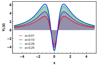
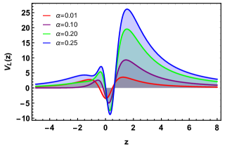
Figure 1: The effective potential for $\lambda=p=\xi=1$, and various values of the modified gravity parameter $\alpha$, for two cases of the $f(T,B)$ function, i.e., $f_{1}$ of (24), and $f_{2}$ of (25).

For the first choice of $f_{1}$, the effective potential (II.2) exhibits a standard behavior commonly discussed in the literature, portraying a perfectly symmetric brane (see $f_{1}$ of Fig. 1). This outcome is significant as it ensures the localization of fermionic modes, thereby validating the physical viability of our model. Moving forward, we observe how variations in the geometry of the model influence the potential’s shape. Increasing the parameter $\alpha$ enhances both the potential barriers and the depth of the potential well. This feature suggests that a greater contribution from the boundary term in our model enhances the localization of fermionic modes on the brane.

Our second choice, $f_{2}$, represents a novel aspect of this work, illustrating how the underlying geometry induces defects in brane symmetry. As depicted in $f_{2}$ of Fig. 1, when $\alpha\rightarrow 0$, the potential exhibits a perfect and symmetric solution. However, as the influence of the boundary term on the model increases, the potential solution deforms, showing slight asymmetry. Importantly, the likelihood of localizing fermionic modes is higher on the right side of the brane. This asymmetry signifies a distorted brane solution, demonstrating that model geometry can indeed induce deformations on the brane. Notably, similar results have been observed in other studies Battisti:2008am ; Perez-Payan:2011cvf ; Sabido:2015xfk ; Lopez:2017xaz ; Lopez-Picon:2023rhc .

In the following subsections we investigate the massless and massive fermionic modes separately.

II.2.1 Massless modes

Similarly to the Yukawa-type coupling scenario, the specific form of the non-minimal coupling $f(T,B)$ plays a crucial role in governing the dynamics of the Kaluza-Klein states. Massless modes, also known as zero modes, exhibit the following form

$$\varphi_{R0,L0}(z)\propto\exp{\Bigg{[}\pm\int\xi f(T,B)e^{A}dz\Bigg{]}},$$ (26)

owing to the supersymmetric structure of the potentials (II.2).

To ascertain whether the zero modes can indeed be localized on the brane, we need to verify whether the normalization condition for the zero modes is satisfied, namely whether we have that

$$\int\varphi_{R0,L0}(z)^{2}dz<\infty.$$ (27)

Given that $f(T,B)e^{A}|_{z\rightarrow\pm\infty}\rightarrow 0$, only the left-handed massless mode is confined to the brane (for positive $\xi$), a feature shared by Yukawa coupling models Yang2012 . Therefore, defining $p=1$, we can derive a straightforward expression for the warp factor in conformal coordinates, namely $A(z)=-\ln\sqrt{1+\lambda^{2}z^{2}}$. As $z$ tends to infinity, $e^{A}\rightarrow 1/\lambda|z|$, consequently, one has

$$\varphi_{L0}(z\rightarrow\pm\infty)\rightarrow|z|^{-\frac{\xi}{\lambda}f(T,B)|_{\infty}},$$ (28)

where $f(T,B)|_{\infty}=c$. If the normalization condition holds, we obtain the following equivalent condition

$$\int|z|^{-2\frac{\xi}{\lambda}f(T,B)|_{\infty}}dz<\infty.$$ (29)

The above integral converges only when $\xi>\lambda/2f(T,B)|_{\infty}$, implying that the left-chirality zero modes can be localized on the brane under this condition.

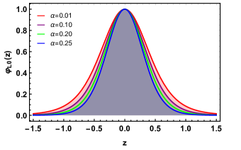
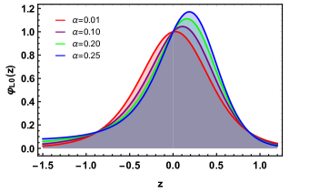
Figure 2: The massless modes for $\lambda=p=\xi=1$, and various values of the modified gravity parameter $\alpha$, for two cases of the $g(T,B)$ function, namely, $g_{1}$ of (24), and $g_{2}$ of (25).

In Fig. 2 we present the massless modes for the two choices of the $f(T,B)$ function. As we observe, the massless fermionic modes are well localized in our model. We mention that only the left-chirality fermions are localized in the brane. For $f_{1}$ case, the massless fermions feel the changes in the effective potential as $\alpha$ increases, and thus the massless modes become more localized in the brane (see $f_{1}$). Concerning the second case $f_{2}$, note that when $\alpha\rightarrow 0$ the massless mode appears symmetrically at the origin of the brane. However, when we increase the effect of the boundary term, the zero-mode solutions become deformed and more localized on the right side of the brane (see $f_{2}$). This is an important feature, as these fermions, although localized, are located outside the core of the brane. Thus, this indicates that theoretically these fermions could only be detected on one (right) side of the brane. This is one of the important results of the present work, since it may correspond to a possible observable of these fermionic particles and thus an indication for extra dimensions.

II.2.2 Massive modes

Let us now proceed to the determination of the massive fermionic modes. To achieve this, considering the even symmetry of the effective potentials illustrated in Fig. 1, we will numerically solve equations (II.2). It is crucial to note that the resulting wave functions will exhibit either even or odd symmetry. Consequently, the boundary conditions are set as follows

$$\varphi_{even}(0) = c,\ \ \partial_{z}\varphi_{even}(0)=0,$$

$$\varphi_{odd}(0) = 0,\ \ \partial_{z}\varphi_{odd}(0)=c,$$ (30)

where $c$ is a constant Almeida2009 ; Liu2009 ; Liu2009a . Here, $\varphi_{even}$ and $\varphi_{odd}$ denote the even and odd parity modes of $\varphi_{R,L}(z)$, respectively.

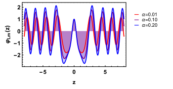
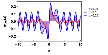
Figure 3: The massive modes for $\lambda=p=\xi=1$, for the $f_{1}$ case of (24) and various values of the modified gravity parameter $\alpha$, for even case (a), and odd case (b).

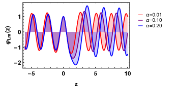
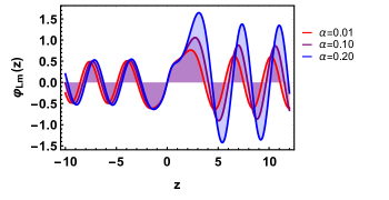
Figure 4: Same as Fig. 3 but for the $f_{2}$ case of (25).

As observed, massive fermionic modes typically resemble free wave solutions. This resemblance stems from the substantial energy that these massive fermions possess, ensuring that very massive fermions (high energy) tend to escape into the extra dimension. However, it is important to note that despite their tendency to escape into the bulk, these fermions can still sense geometric modifications near the brane core. In Fig. 3, we depict the solutions of the massive fermionic modes for the case $f_{1}$ of (24). It is evident that as the parameter $\alpha$ increases, the oscillations in the brane core undergo significant modifications. Thus, even though these modes are not localized on the brane, their influence can be detected there, potentially affecting measurements such as gravitational wave detections, leading to noise effects.

Moreover, the massive fermionic modes for $f_{2}$ exhibit asymmetric behavior, as illustrated in Fig. 4. Increasing the influence of the boundary term in the model results in heightened oscillations on the right side of the brane. Noticeably, in this scenario, the brane behaves akin to a barrier, decreasing the likelihood of fermions crossing to the left side.

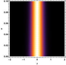
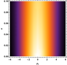
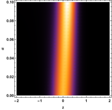
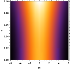
Figure 5: The entropy densities for $\lambda=p=\xi=1$. The left panels correspond to position space (32), while the right panels, correspond to momentum space (33). Additionally, the upper panels, correspond to the case $f_{1}$ of (24), while the lower panels correspond to the case $f_{2}$ of (25). Lighter regions correspond to higher probability of appearance than the darker ones.

III Information measures

In this section, we apply information measures as a tool to further analyze how geometry influences the localization of fermions on the brane. Specifically, we utilize Shannon information entropy theory and Fisher information measurement theory, focusing on the massless case. Additionally, for the massive modes, we employ the relative probability formalism.

III.1 Shannon theory

Shannon’s entropy theory is basic in information theory Shannon . Its power lies in offering insights into particle localization via the system probability density $|\varphi_{L0,R0}(z)|^{2}$, and thus it can explore the loss of information or noise between a transmitting and receiving source. We start by applying the Fourier transformation to the massless mode function, expressed as

$$|\varphi_{L0,R0}(p_{z})|^{2}=\frac{1}{\sqrt{2\pi}}\int_{-\infty}^{\infty}|\varphi_{L0,R0}(z)|^{2},\text{e}^{-ipz}dz,$$ (31)

where $p_{z}$ is the coordinate of momentum space or reciprocal space. We proceed to define Shannon entropy for both position and momentum spaces, as

$$S_{z} = -\int_{-\infty}^{\infty}\rho_{s}(z)dz,$$ (32)

$$S_{p_{z}} = -\int_{-\infty}^{\infty}\rho_{s}(p_{z})dp_{z},$$ (33)

where

$$\rho_{s}(z) = |\varphi_{L0,R0}(z)|^{2}\ln|\varphi_{L0,R0}(z)|^{2},$$ (34)

$$\rho_{s}(p_{z}) = |\varphi_{L0,R0}(p_{z})|^{2}\ln|\varphi_{L0,R0}(p_{z})|^{2},$$ (35)

are the entropy densities of the system.

Relations (32), (33) yield an uncertainty relation, known as the Beckner, Bialynicki-Birula, Mycielski (BBM) relation Beckner ; Bialy . The important aspect of this entropy uncertainty relation is its effectiveness as an alternative to the Heisenberg uncertainty principle. The BBM uncertainty relation is mathematically expressed as

$$S_{z}+S_{p_{z}}\geq D(1+\text{ln}\pi),$$ (36)

where $D$ denotes the dimensions capable of discerning changes in the system information. In our model, only the extra dimension perceives entropy modifications within the system, and therefore $D=1$.

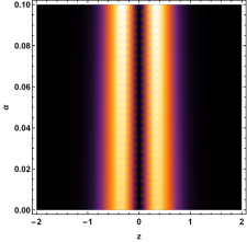
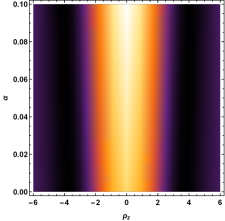
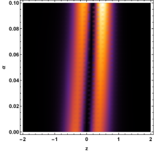
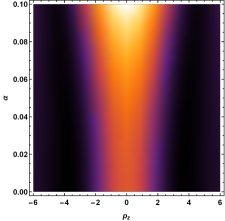
Figure 6: The information densities for $\lambda=p=\xi=1$. The left panels correspond to position space (37), while the right panels correspond to momentum space (38). Additionally, the upper panels correspond to the case $f_{1}$ of (24), while the lower panels correspond to the case $f_{2}$ of (25). Lighter regions correspond to higher probability of appearance than the darker ones.

The entropy densities can provide information on the behavior of the fermions and their possible location. In Fig. 5, we present the shape of the entropy density for our two choices of the $f(T,B)$ modified gravity function of (24) and (25). Lighter regions correspond to a higher probability of appearance than darker ones. For the $f_{1}$ case, the entropy density in position space appears linearly at the origin of the brane, while in momentum space, the density appears thicker. In contrast, for the $f_{2}$ case, the entropy density deviates from the origin as we increase the value of $\alpha$.

Lastly, Shannon entropy provides additional information about the possible location of the massless fermions. We numerically compute the equations and present the results in Table 1. Increasing the effect of the boundary term decreases Shannon entropy in position space, indicating reduced information loss and increased certainty about the fermion’s location. However, Shannon entropy in momentum space increases, reflecting greater uncertainty about the particle momentum with larger information losses, consistent with the uncertainty principle and satisfying the BBM relation. Finally, the total entropy sum increases with larger $\alpha$ values, indicating increased total information loss about the fermion.

Table 1: Shannon entropy values in position and momentum space for the two cases of the $f(T,B)$ function, with $\xi=p=\lambda=1$.

$n$	$\alpha$	$S_{z}$	$S_{p_{z}}$	$S_{z}+S_{p_{z}}$
$g_{1}$	0.01	0.21998	2.28577	2.50575
	0.10	0.20899	2.30903	2.51802
	0.20	0.16477	2.40538	2.57015
	0.25	0.15473	2.42789	2.58262
$g_{2}$	0.01	0.22122	2.28318	2.50441
	0.10	0.22023	2.28722	2.50745
	0.20	0.19858	2.37979	2.57837
	0.25	0.19099	2.41879	2.60978

III.2 Fisher theory

Fisher information theory is a useful tool of quantifying the information content carried by an observable random variable about an unknown parameter Fisher . One key aspect of this theory is its connection to the probability density of an information system, which can also be correlated with the probability density observed in quantum systems. The informational density associated with Fisher theory is expressed as

$$\rho_{F}(z) = |\varphi_{L0,R0}(z)|^{2}\bigg{[}\frac{d}{dz}\ln|\varphi_{L0,R0}(z)|^{2}\bigg{]}^{2},$$ (37)

$$\rho_{F}(p_{z}) = |\varphi_{L0,R0}(p_{z})|^{2}\bigg{[}\frac{d}{dp_{z}}\ln|\varphi_{L0,R0}(p_{z})|^{2}\bigg{]}^{2}.$$ (38)

Consequently, for the probability density of a continuous system, Fisher information can be computed for position space $F_{z}$ and momentum space $F_{p_{z}}$, namely

$$F_{z} = \int_{-\infty}^{\infty}\rho_{F}(z)dz,$$ (39)

$$F_{p_{z}} = \int_{-\infty}^{\infty}\rho_{F}(p_{z})dp_{z}.$$ (40)

We mention that these probabilistic measures of information also propose an alternative to the Heisenberg uncertainty principle, namely

$$\sigma_{z}\sigma_{p_{z}}\geq\frac{1}{(F_{z}F_{p_{z}})^{\frac{1}{2}}}\geq\frac{1}{2},$$ (41)

leading to

$$F_{z}F_{p_{z}}\geq 4,$$ (42)

where $\sigma_{z}^{2}=\langle z^{2}\rangle-\langle z\rangle^{2}$ and $\sigma_{p_{z}}^{2}=\langle p_{z}^{2}\rangle-\langle p_{z}\rangle^{2}$.

Information densities, akin to information entropy, reveal the possible location of the fermions. In Fig. 6, we present the behavior of information density for our two choices of the $f(T,B)$ modified gravity function of (24) and (25). In the $f_{1}$ case, we observe that regions with low information density separate regions with higher information density. Additionally, in position space, there are two peaks in information density, while in momentum space, there is only one. For the $f_{2}$ case, the information density illustrates the deformation of the brane in both position and momentum spaces.

We numerically compute the equations and present the results in Table 2. As observed, increasing the effect of the boundary term enhances the information measures in position space. However, in momentum space, the opposite occurs such that the total sum of information measures decreases as $\alpha$ increases. Larger Fisher information measures correspond to higher probabilities of receiving information from the fermion (indicating less information loss and noise), thereby increasing certainty about the fermion’s location.

Table 2: Fisher information values in position and momentum space for the two cases of the $f(T,B)$ function, with $\xi=p=\lambda=1$.

$n$	$k$	$F_{z}$	$F_{p_{z}}$	$F_{z}F_{p_{z}}$
$g_{1}$	0.01	2.81545	7.74121	21.7949
	0.10	2.87569	7.39004	21.2514
	0.20	3.13204	6.02243	18.8623
	0.25	3.19351	5.72364	18.2785
$g_{2}$	0.01	2.80880	7.91084	22.2199
	0.10	2.81871	7.22346	20.3608
	0.20	3.05356	5.75099	17.5609
	0.25	3.15738	5.29128	16.7065

III.3 Relative probability

Let us now focus on the massive fermionic modes. Although they do not reside on the brane, certain heavy states may exhibit significant presence in close proximity to it Almeida2009 . These substantial states manifest when the potentials near the brane form a potential well, accommodating masses $m^{2}$ within the highest value of the potential barrier Liu2009 ; Liu2009a . We refer to these occurrences as resonant modes, which arise from the analogous quantum mechanical structure of heavy modes Almeida2009 ; Liu2009 ; Liu2009a .

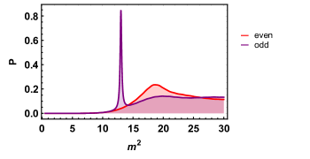
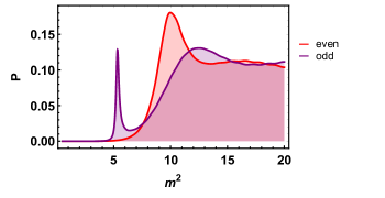
Figure 7: The relative probability (43) for $\xi=p=\lambda=1$ and $\alpha=0.1$, for two cases of the $g(T,B)$ function, namely: $g_{1}$ of (24), and $g_{2}$ of (25).

To pinpoint the solutions of the Schrödinger-like equation (II.2) with significant amplitudes near the brane, we apply the resonance method. The relative probability $P(m)$ of detecting a particle with mass $m$ within a narrow band $2z_{b}$ is given by Almeida2009 ; Liu2009 ; Liu2009a

$$P_{R,L}(m)=\frac{\int_{-z_{b}}^{z_{b}}|\varphi_{R,L}(z)|^{2}dz}{\int_{-z_{\text{max}}}^{z_{\text{max}}}|\varphi_{R,L}(z)|^{2}dz},$$ (43)

where $z_{\text{max}}$ represents the domain boundaries. While larger values of the parameter $z_{b}$ maintain consistency in locating the resonance peaks, smaller $z_{b}$ values prove more adept at pinpointing these peaks.

We numerically compute the equations, and in Fig. 7, we illustrate the relative probabilities for our model. The peaks in relative density delineate resonant modes with the highest likelihood of locating massive fermions on the brane. For the $f_{1}$ case, the peak occurs around $12<m^{2}<14$ (odd), while for the $f_{2}$ case, the peak is around $4.5<m^{2}<6.0$ (odd). This indicates that in this model, massive fermions with these mass spectra have a greater chance of being detected on the brane.

IV Conclusions

In this work, we investigated the dynamics of fermion localization within the framework of $f(T,B)$ gravity. Starting from the Dirac action for a fermion with spin $1/2$ embedded in a 5-dimensional spacetime governed by torsional $f(T,B)$ gravity, we formulated the Dirac equation and explored its solutions under various non-minimal coupling functions.

We examined two realistic forms of the non-minimal coupling function $f(T,B)$, i.e., $f_{1}(T,B)=\sqrt{-T-\alpha(B)}$ and $f_{2}(T,B)=\sqrt{-T}-\alpha B$. Our analysis revealed distinct behaviors, highlighting implications for the localization of both massless and massive fermionic modes on the brane. Particularly, we observed how geometric deformations induced in the brane can influence the localization of fermionic modes, potentially providing avenues for experimental detection of these particles.

Furthermore, we employed probabilistic measures-Shannon entropy theory, Fisher information theory, and relative probability-to investigate the localization of massless and massive fermionic modes. Our analysis provided insights into the information content and uncertainty associated with fermion localization on the brane, offering a nuanced understanding of the interplay between position and momentum spaces.

In summary, this study represents a significant step toward comprehending the impact of modified gravity on fermion localization in brane world scenarios. The observed effects could potentially serve as probes for torsional modifications and may open new avenues for exploring holography and brane cosmography.

References

- (1) T. Kaluza, Sitzungsber. Preuss. Akad. Wiss. Berlin (Math. Phys. ) 1921, 966-972 (1921).
- (2) O. Klein, Nature 118, 516 (1926).
- (3) N. Arkani-Hamed, S. Dimopoulos and G. R. Dvali, Phys. Lett. B 429, 263-272 (1998).
- (4) L. Randall and R. Sundrum, Phys. Rev. Lett. 83, 4690 (1999).
- (5) L. Randall and R. Sundrum, Phys. Rev. Lett. 83, 3370 (1999).
- (6) S. H. Dong, Wave equations in higher dimensions, Springer, Dordrecht, Heidelberg, London, New York, 2011.
- (7) R. Gregory, V. A. Rubakov and S. M. Sibiryakov, Phys. Rev. Lett. 84, 5928-5931 (2000).
- (8) T. Appelquist, H. C. Cheng and B. A. Dobrescu, Phys. Rev. D 64, 035002 (2001).
- (9) G. R. Dvali, G. Gabadadze and M. Porrati, Phys. Lett. B 485, 208-214 (2000).
- (10) O. DeWolfe, D. Z. Freedman, S. S. Gubser and A. Karch, Phys. Rev. D 62, 046008 (2000).
- (11) M. Gremm, Phys. Lett. B 478, 434 (2000).
- (12) C. Csaki, J. Erlich, T. J. Hollowood and Y. Shirman, Nucl. Phys. B 581, 309-338 (2000).
- (13) M. Gremm, Phys. Rev. D 62, 044017 (2000).
- (14) V. Dzhunushaliev, V. Folomeev and M. Minamitsuji, Rept. Prog. Phys. 73, 066901 (2010).
- (15) V. Dzhunushaliev and V. Folomeev, Gen. Rel. Grav. 43, 1253-1261 (2011).
- (16) A. Herrera-Aguilar, D. Malagon-Morejon, R. R. Mora-Luna and U. Nucamendi, gap, ” Mod. Phys. Lett. A 25, 2089-2097 (2010).
- (17) V. Dzhunushaliev, V. Folomeev, D. Singleton and S. Aguilar-Rudametkin, Phys. Rev. D 77, 044006 (2008).
- (18) M. Gogberashvili and D. Singleton, Phys. Rev. D 69, 026004 (2004).
- (19) M. Gogberashvili and D. Singleton, Phys. Lett. B 582, 95-101 (2004).
- (20) W. D. Goldberger and M. B. Wise, Phys. Rev. Lett. 83 (1999), 4922.
- (21) D. Bazeia, A. R. Gomes, L. Losano and R. Menezes, Phys. Lett. B 671 (2009), 402.
- (22) W. J. Geng and H. Lu, Phys. Rev. D 93, no.4, 044035 (2016).
- (23) V. Dzhunushaliev and V. Folomeev, Gen. Rel. Grav. 44, 253-261 (2012).
- (24) E. Abdalla, G. Franco Abellán, A. Aboubrahim, A. Agnello, O. Akarsu, Y. Akrami, G. Alestas, D. Aloni, L. Amendola and L. A. Anchordoqui, et al. JHEAp 34, 49-211 (2022).
- (25) E. N. Saridakis et al. [CANTATA], Spinger (2021), [arXiv:2105.12582 [gr-qc]].
- (26) S. Capozziello and M. De Laurentis, Phys. Rept. 509, 167 (2011).
- (27) Y. F. Cai, S. Capozziello, M. De Laurentis and E. N. Saridakis, Rept. Prog. Phys. 79, 106901 (2016).
- (28) A. A. Starobinsky, Phys. Lett. B 91, 99 (1980).
- (29) A. De Felice and S. Tsujikawa, Living Rev. Rel. 13, 3 (2010).
- (30) S. Capozziello, Int. J. Mod. Phys. D 11, 483-492 (2002).
- (31) S. Nojiri and S. D. Odintsov, Phys. Lett. B 631, 1 (2005).
- (32) A. De Felice and S. Tsujikawa, Phys. Lett. B 675, 1-8 (2009).
- (33) P. Asimakis, S. Basilakos and E. N. Saridakis, Eur. Phys. J. C 84, no.2, 207 (2024).
- (34) D. Lovelock, J. Math. Phys. 12, 498 (1971).
- (35) N. Deruelle and L. Farina-Busto, Phys. Rev. D 41, 3696 (1990).
- (36) G. W. Horndeski, Int. J. Theor. Phys. 10, 363-384 (1974).
- (37) A. De Felice and S. Tsujikawa, Phys. Rev. D 84, 124029 (2011).
- (38) C. Deffayet, X. Gao, D. A. Steer and G. Zahariade, Phys. Rev. D 84, 064039 (2011).
- (39) T. Kobayashi, M. Yamaguchi and J. Yokoyama, Phys. Rev. Lett. 105, 231302 (2010).
- (40) A. De Felice and S. Tsujikawa, JCAP 02, 007 (2012).
- (41) E. V. Linder, Phys. Rev. D 81, 127301 (2010) [erratum: Phys. Rev. D 82, 109902 (2010)].
- (42) S. H. Chen, J. B. Dent, S. Dutta and E. N. Saridakis, Phys. Rev. D 83, 023508 (2011).
- (43) G. Kofinas and E. N. Saridakis, Phys. Rev. D 90, 084044 (2014).
- (44) G. Kofinas and E. N. Saridakis, Phys. Rev. D 90, 084045 (2014).
- (45) S. Bahamonde, C. G. Böhmer and M. Wright, Phys. Rev. D 92, no.10, 104042 (2015).
- (46) S. Bahamonde and S. Capozziello, Eur. Phys. J. C 77, no.2, 107 (2017).
- (47) C. Q. Geng, C. C. Lee, E. N. Saridakis and Y. P. Wu, Phys. Lett. B 704, 384-387 (2011).
- (48) S. Bahamonde, K. F. Dialektopoulos and J. Levi Said, Phys. Rev. D 100, no.6, 064018 (2019).
- (49) S. Bahamonde, K. F. Dialektopoulos, M. Hohmann and J. Levi Said, Class. Quant. Grav. 38, no.2, 025006 (2020).
- (50) S. Capozziello, M. Caruana, J. Levi Said and J. Sultana, JCAP 03, 060 (2023).
- (51) R. Aldrovandi and J. G. Pereira, Teleparallel Gravity: An Introduction, (Springer, Berlin, 2013).
- (52) G. A. R. Franco, C. Escamilla-Rivera and J. Levi Said, Eur. Phys. J. C 80 (2020), 677.
- (53) C. Escamilla-Rivera and J. Levi Said, Class. Quant. Grav. 37 (2020), 165002.
- (54) S. Bahamonde, M. Zubair and G. Abbas, Phys. Dark Univ. 19 (2018), 78.
- (55) H. Abedi and S. Capozziello, Eur. Phys. J. C 78 (2018), 474.
- (56) G. Farrugia, J. Levi Said, V. Gakis and E. N. Saridakis, Phys. Rev. D 97, no.12, 124064 (2018).
- (57) I. Soudi, G. Farrugia, V. Gakis, J. Levi Said and E. N. Saridakis, Phys. Rev. D 100, no.4, 044008 (2019).
- (58) V. Gakis, M. Krššák, J. Levi Said and E. N. Saridakis, Phys. Rev. D 101, no.6, 064024 (2020).
- (59) M. Caruana, G. Farrugia and J. Levi Said, Eur. Phys. J. C 80 (2020), 640.
- (60) A. Pourbagher and A. Amani, Mod. Phys. Lett. A 35 (2020), 2050166.
- (61) S. Bahamonde, V. Gakis, S. Kiorpelidi, T. Koivisto, J. Levi Said and E. N. Saridakis, Eur. Phys. J. C 81 (2021), 53.
- (62) N. Azhar, A. Jawad and S. Rani, Phys. Dark Univ. 30 (2020), 100724.
- (63) S. Bahamonde, M. Caruana, K. F. Dialektopoulos, V. Gakis, M. Hohmann, J. Levi Said, E. N. Saridakis and J. Sultana, Phys. Rev. D 104, no.8, 084082 (2021).
- (64) S. Bhattacharjee, Phys. Dark Univ. 30 (2020), 100612.
- (65) M. Mylova, J. Levi Said and E. N. Saridakis, Class. Quant. Grav. 40, no.12, 125002 (2023).
- (66) J. Yang, Y. -L. Li, Y. Zhong and Y. Li, Phys. Rev. D 85, 084033 (2012).
- (67) A. R. P. Moreira, J. E. G. Silva and C. A. S. Almeida, Eur. Phys. J. C 81, no.4, 298 (2021).
- (68) Y. N. Obukhov and J. G. Pereira, Phys. Rev. D 67, 044016 (2003)
- (69) S. C. Ulhoa, A. F. Santos and F. C. Khanna, Gen. Rel. Grav. 49, 54 (2017).
- (70) C. A. S. Almeida, M. M. Ferreira, Jr., A. R. Gomes and R. Casana, Phys. Rev. D 79, 125022 (2009).
- (71) D. M. Dantas, D. F. S. Veras, J. E. G. Silva and C. A. S. Almeida, Phys. Rev. D 92, 104007 (2015).
- (72) M. V. Battisti, J. Phys. Conf. Ser. 189, 012005 (2009).
- (73) S. Pérez-Payán, M. Sabido and C. Yee-Romero, Phys. Rev. D 88, no.2, 027503 (2013).
- (74) M. Sabido and C. Yee-Romero, acceleration, ” Phys. Lett. B 757, 57-60 (2016).
- (75) J. L. López, M. Sabido and C. Yee-Romero, Phys. Dark Univ. 19, 104-108 (2018).
- (76) J. L. López-Picón, M. Sabido and C. Yee-Romero, Phys. Lett. B 849, 138420 (2024).
- (77) Y. X. Liu, J. Yang, Z. H. Zhao, C. E. Fu and Y. S. Duan, Phys. Rev. D 80, 065019 (2009).
- (78) Y. X. Liu, H. T. Li, Z. H. Zhao, J. X. Li and J. R. Ren, JHEP 10, 091 (2009).
- (79) C. E. Shannon, Bell Syst. Tech. J. 27, no.3, 379-423 (1948).
- (80) W. Beckner, Ann. Math. 102, 159 (1975).
- (81) I. Białynicki-Birula and J. Mycielski, Commun. Math. Phys. 44, no.2, 129-132 (1975).
- (82) Fisher, R. A.: Theory of Statistical Estimation. Math. Proc. Camb. Philos. Soc. 22, 700 (1925).