Resonant excitation of quasinormal modes of black holes
Abstract
We elucidate that a distinctive resonant excitation between quasinormal modes (QNMs) of black holes emerges as a universal phenomenon at avoided crossing near exceptional point through high-precision numerical analysis and theory of QNMs based on the framework of non-Hermitian physics. This resonant phenomenon not only allows us to decipher a long-standing mystery concerning the peculiar behaviors of QNMs but also stands as a novel beacon for characterizing black hole spacetime geometry. Our findings pave the way for rigorous examinations of black holes and the exploration of new physics in gravity.
Introduction. The last decade has witnessed the advent of gravitational wave (GW) astronomy, opening a new window to the universe, especially in the dynamical and strong-field regime near black holes Abbott et al. (2016); Aasi et al. (2015); Acernese et al. (2015); Akutsu et al. (2021). General relativity predicts that black holes are the simplest astrophysical objects in the universe since the only rotating astrophysical black hole solution that satisfies the Einstein equation is the Kerr spacetime Israel (1967); Carter (1971); Hawking (1972), characterized solely by mass and spin. Remnant black holes after binary black hole mergers are expected to settle into the state of a Kerr black hole, emitting ringdown GWs. Linear perturbation theory predicts that the ringdown GWs are described by a linear combination of intrinsic exponentially damped sinusoids known as quasinormal modes (QNMs) Vishveshwara (1970); Press (1971); Teukolsky (1973); Chandrasekhar and Detweiler (1975). Their timescales and amplitudes are governed by complex frequencies and excitation factors Leaver (1985, 1986a, 1986b); Sun and Price (1988); Nollert and Schmidt (1992); Nollert and Price (1999); Andersson (1995, 1997); Glampedakis and Andersson (2001, 2003), also determined solely by mass and spin, playing a central role in the black hole spectroscopy program Detweiler (1980); Echeverria (1989); Finn (1992); Dreyer et al. (2004); Berti et al. (2006). Despite extensive efforts to better understand them, the peculiar behaviors of QNMs reflecting changes in black hole parameters have remained elusive Kokkotas and Schmidt (1999); Nollert (1999); Berti et al. (2009); Konoplya and Zhidenko (2011).
In this Letter, we reveal the emergence of the resonant excitation phenomenon associated with an avoided crossing of QNMs near the exceptional point (EP). The avoided crossing in quantum mechanics, also known as level repulsion, is a phenomenon where two energy eigenvalues cannot coincide unless a certain condition is satisfied Hund (1927); von Neuman and Wigner (1929); Landau and Lifshitz (1977); Arnold (1978). It plays a pivotal role in experiments and observations across vast fields of physical science Ashcroft and Mermin (1976); Landau (1932); Zener (1932); Majorana (1932); Stückelberg (1932); Ivakhnenko et al. (2023); Purcell (1946); Herzberg (1991); Smirnov (2003); Wurm (2017); Giganti et al. (2018). The EP Kato (1995); Özdemir et al. (2019); Wiersig (2020); Parto et al. (2021); Ding et al. (2022), a branch point singularity in the complex eigenvalue plane, is crucial in non-Hermitian physics El-Ganainy et al. (2018); Bergholtz et al. (2021); Ashida et al. (2021), where avoided crossing occurs in its vicinity Heiss (2000, 2012). With these concepts, we formulate the resonance of QNMs and provide novel perspectives for exploring gravity. We employ geometric units with throughout.
Kerr QNM frequencies and excitation factors. We first reveal the emergence of the resonance of Kerr QNMs at avoided crossing and identify their unique features. Linear perturbation theory in general relativity predicts that the ringdown GW strain at far distance from perturbed Kerr black hole is given by a superposition of QNM damped sinusoids Vishveshwara (1970); Press (1971); Teukolsky (1973); Chandrasekhar and Detweiler (1975):
| (1) |
in a decomposition in terms of spin-weighted spheroidal harmonics Teukolsky (1972, 1973); Press and Teukolsky (1973). While a complex factor involves an integral depending on the initial condition, recent studies suggest that for each multipole does not strongly depend on the overtone index and black hole spin Oshita (2021); Cheung et al. (2024). Therefore, the ringdown GWs are mainly governed by complex QNM frequencies and excitation factors defined by Leaver (1986b)
| (2) |
with asymptotic amplitudes and for the outgoing and ingoing waves, respectively. and depend only on mass and spin of the black hole. Since the mass dependency is a simple scaling, the dependency on a dimensionless spin parameter is of primary interest.
We revisit numerical calculation of the QNM frequencies and excitation factors of Kerr black holes. We closely follow the strategy adopted in Zhang et al. (2013) and implement some technical improvements to achieve high-precision calculation up to higher overtones which will be presented elsewhere 111In addition, we also correct some errors found in an intermediate step of Zhang et al. (2013). Consequently, our results of excitation factors and the ones in Zhang et al. (2013) differ for a factor of .. The dataset is publicly available Motohashi (2024a).
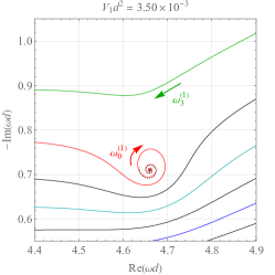
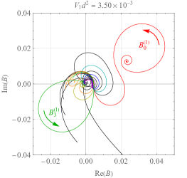
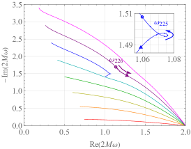
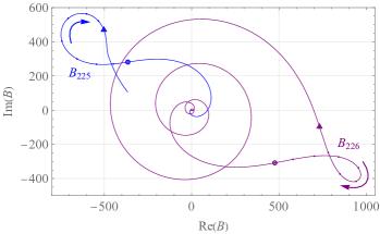
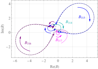
For multipole of GWs, most of the Kerr QNM frequencies uniformly migrate towards the accumulation point at Detweiler (1980); Glampedakis and Andersson (2001); Cardoso (2004); Hod (2008); Yang et al. (2013a, b). However, as depicted in Fig. 1, only the fifth overtone suddenly turns over at with making a small knot-shape loop and heads towards an isolated point far from the accumulation point. This behavior was first pointed out by Onozawa Onozawa (1997) about three decades ago and has been confirmed by other work Yang et al. (2013b); Cook and Zalutskiy (2014), but the physical reason has been veiled. While it has been implicitly assumed that the fifth overtone solely behaves in a strange manner, here we point out that, while less manifest, the trajectory of the sixth overtone QNM frequency is slightly distorted when it passes near the fifth overtone at .
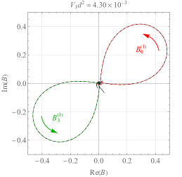
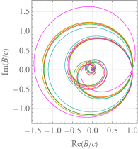
On the other hand, it was recently found that the absolute values of and become large for high-spin Kerr black holes Giesler et al. (2019); Oshita (2021), despite the fact that the excitation factors tend to zero at the extremal spin Ferrari and Mashhoon (1984); Berti and Cardoso (2006); Zhang et al. (2013) and asymptotically scale as for higher overtones Andersson (1997); Berti and Cardoso (2006). Again, the physical reason has been unclear. However, when viewed on the complex plane in Fig. 1, we notice that the excitation factors actually exhibit a suggestive behavior. While other overtones follow spiral trajectories, it turns out that and are against the spirals and are enhanced in almost opposite directions at .
The implications of these observations are two-fold: First, this phenomenon should be viewed as occurring in a pair of two modes rather than a single mode. Second, there should be an underlying interplay between the turning/distortion of the QNM frequencies and the strong excitations.
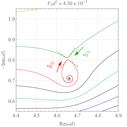
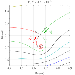
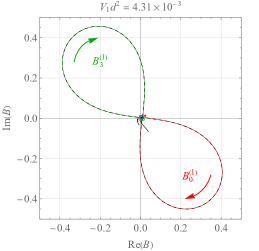
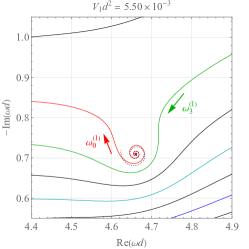
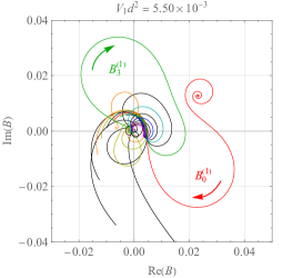
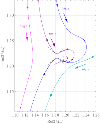
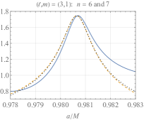
Actually, a similar phenomenon occurs more manifestly for higher multipoles. In Fig. 2, we see that modes exhibit the distinctive behaviors successively between multiple pairs. Among them the pair of and is the most manifest case, exhibiting a sharp repulsion between the two QNM frequencies 222Such repulsion was also observed in the QNMs of scalar field in Kerr Yang et al. (2013b), (anti-)de Sitter black holes Jansen (2017); Davey et al. (2022); Kinoshita et al. (2024), and charged black holes Dias et al. (2022a, b); Davey et al. (2024).. In Fig. 2, we also note that the mild repulsion between and overtones seems to be a trigger of the looping trajectory of the sixth overtone found in Onozawa (1997); Cook and Zalutskiy (2014). Further, during these peculiar behaviors of QNM frequencies, the corresponding pairs of excitation factors exhibit symmetric amplifications. The sharper the repulsion between two QNM frequencies are, the more strongly and clearly point symmetrically the corresponding pair of excitation factors are amplified.
Interestingly, for the most manifest case in Fig. 2, we find that the QNM frequencies and excitation factors almost follow the hyperbola and the lemniscate of Bernoulli, respectively. When written down in the polar coordinates with , the hyperbola and lemniscate are inverses of each other. Albeit approximate, it is remarkable that such intimately related curves are inherent in QNM spectrum of Kerr GWs.
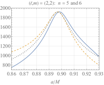
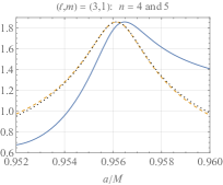
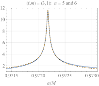
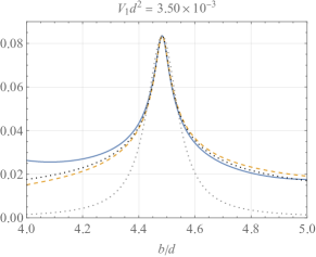
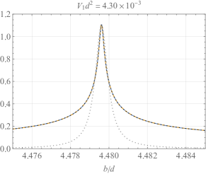
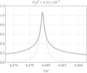
We show in Fig. 3 that the inverse proportionality between the difference of excitation factors and the difference of QNM frequencies is actually a common feature of the pair excitations, providing insight that they belong to the same underlying phenomenon. As expected, the inverse proportionality is more manifest for the case of sharper repulsion and stronger excitation. Further, we find that the peaks in Fig. 3, especially the sharp ones, demonstrate an excellent agreement with a quarter-power Lorentzian , where with positive parameters , rather than the Lorentzian itself. Not only the absolute value, we also confirm that a product remains almost constant as a complex number during the resonant excitation.
We find that this phenomenon ubiquitously occurs for Kerr QNMs, i.e., GWs with other multipoles, and scalar and electromagnetic fields. Further, even in QNMs away from Kerr, we find that the resonances with the same features show up (see Supplemental Material). These are tantalizing hints to a universal nature of QNMs.
Theory of quasinormal modes. Below we provide a theoretical explanation for this phenomenon by developing a theory of QNMs. Let us consider the QNMs of a general master equation for perturbations around a black hole after Fourier and harmonic expansions,
| (3) |
where is an effective potential and denotes the tortoise coordinate with corresponding to the spatial infinity and event horizon of the black hole, respectively. For nonrotating black holes, Regge and Wheeler (1957); Zerilli (1970) and hence (3) reads with an effective Hamiltonian , which is analogous to the Schrödinger equation in quantum mechanics. For radial perturbation equation of rotating black holes, depends on and other parameters Teukolsky (1972, 1973), so (3) defines a nonlinear eigenvalue problem. changes as the spin parameter varies, causing the migration of QNM frequencies.
A crucial difference of QNMs from the bound state in quantum mechanics originates from the boundary condition. Instead of decaying at infinity, the QNM wave function is required to satisfy the in/outgoing wave condition as . This Siegert boundary condition discretizes the QNM eigenvalues as complex number with negative imaginary part. Hence, the QNM wave function diverges at (when viewed at constant time hypersurface), and the standard inner product for bound states is not well-defined for QNMs. Several kinds of definitions of the inner product for QNMs of black holes have been considered Ching et al. (1995); Leung et al. (1997, 1998); Yang et al. (2015); Zimmerman et al. (2015); Jaramillo et al. (2021); Gasperin and Jaramillo (2022); Yang and Zhang (2023); Green et al. (2023); London (2023); London and Gurevich (2023); Ma and Yang (2024).
In quantum mechanics, this kind of system is known as the Schrödinger problem of open systems and has been utilized for studies of quantum resonances, for which the Hamiltonian is not Hermitian Gamow (1928); Landau and Lifshitz (1977); Kukulin et al. (1989); Moiseyev (2011). More recently, the non-Hermitian physics has been extensively studied both from theoretical and experimental point of view El-Ganainy et al. (2018); Bergholtz et al. (2021); Ashida et al. (2021). Here, we define a regular inner product, or more precisely biorthogonal product, for QNMs inspired by the case of the quantum resonance states Kukulin et al. (1989); More (1971a, b); Sternheim and Walker (1972). It corresponds to a generalization of Ching et al. (1995); Leung et al. (1997, 1998) to the case with (3) including rotating black holes. In this formulation, QNM wave function with eigenvalue corresponds to the resonance state, for which we introduce so-called anti-resonance (or adjoint) state with eigenvalue . We then define the biorthogonal product for QNMs along a contour as
| (4) |
where . From (3), it is straightforward to show that the biorthogonality exactly holds for any , i.e., when . Formally taking the limit , we define the “norm squared” for QNMs as
| (5) |
which is in general complex 333As a special case, if we choose a contour along the real axis, (5) reduces to the Zel’dovich regularization Zel’dovich (1961) (see also earlier work Kapur et al. (1938)).. We can analytically show that satisfies a useful formula Motohashi (2024b)
| (6) |
which allows for an alternative way to calculate the excitation factor defined by (2). The equivalence between (6) and (2) is also numerically crosschecked for various specific cases including Schwarzschild and Kerr black holes. The formula (6) tells us that the excitation factor becomes large when the norm squared becomes small, which precisely occurs at the avoided crossing near the EP.
Resonant excitation at avoided crossing. To investigate how QNM frequencies and excitation factors change when two QNM frequencies get close due to the variation of , let us regard the continuous changes as an accumulation of infinitesimal changes . If a mode is far from degeneracy, it is straightforward to generalize the Rayleigh-Schrödinger-like perturbation theory for resonance state Zel’dovich (1961); Perelomov and Zel’dovich (1998) to QNMs and obtain Motohashi (2024b)
| (7) |
which reveals another role of the excitation factor , i.e., defining the sensitivity of to .
The avoided crossing, where two (or more) eigenvalues are close to degenerate, requires a special care 444Note that the similarity between the avoided crossing and repulsion of QNM eigenvalues was pointed out in Dias et al. (2022a, b); Davey et al. (2024) in the studies of charged black holes. Here we examine QNM frequencies and also excitation factors and derive the resonant excitation.. We employ a simple analysis of bifurcation theory of eigenvalues about EP Heiss (2000); Seyranian and Mailybaev (2003) to capture the essential features of the resonance. We focus on the nonrotating black hole case with 555The rotating black hole case may be investigated by applying a prescription of auxiliary eigenvalue recently employed in Isobe et al. (2024) in the context of the bulk-edge correspondence. and assume that two QNM overtones are close and they are isolated from other QNMs so that we can approximately treat them as a two-level system. Suppose a small change as a part of continuous changes, causing a change of the QNM frequencies , which can be obtained as eigenvalues of the Hamiltonian :
| (8) |
where , with , and . When is negligible, (8) recovers , the result of perturbation theory. On the other hand, are degenerate if is satisfied, which defines EP. Since this condition involves complex variables, it is in general not possible to be satisfied by tuning a single real parameter, resulting the avoided crossing.
Let us consider the case where continuous variation of is driven by a single parameter. At each point except the avoided crossing the perturbation theory is valid, and hence follow . Suppose that the perturbation theory predicts the two modes approach on the same line, for which, denoting and , is a real parameter and and are constant. We also neglect the variation of . The single-parameter degree of freedom of is thus represented by . Denoting , it is straightforward to derive , where is defined by rotation of by . Unless , which requires a tuning of an additional parameter, follows a hyperbolic avoided crossing, and so does itself, since this occurs at a small region near EP. A simple calculation shows at the peak when , which means obeys the quarter-power Lorentzian.
On the other hand, QNM eigenstates associated to are given by and , where is governed by a dimensionless complex parameter . If the two modes are close and then and are satisfied, the eigenstates are almost degenerate , and the norm squared nearly vanish as . These behaviors are nothing but what is expected at EP Özdemir et al. (2019); Wiersig (2020); Parto et al. (2021); Ding et al. (2022). With (6) and (8), we obtain . Hence, the excitation factors are amplified following the inverse of the hyperbola, i.e., the lemniscate of Bernoulli, and the resonance peak obeys the quarter-power Lorentzian.
Conclusions and Discussion. When two QNM frequencies approach on the complex plane, they are anomalously excited. We clarified this resonance phenomenon by developing high-precision numerical analysis and theoretical framework of QNMs in the language of non-Hermitian physics. The resonance of Kerr QNMs not only allows us to decipher a long-standing mystery in black hole physics but also stands as a novel beacon for characterizing black hole spacetime geometry. Deviations from Kerr, whether due to astrophysical effects or correction to general relativity, will manifest in the resonances in QNMs. Our findings thus pave the way for rigorous examinations of black holes and the exploration of new physics in gravity.
Acknowledgments. This work was supported by Japan Society for the Promotion of Science (JSPS) Grants-in-Aid for Scientific Research (KAKENHI) Grant No. JP22K03639.
References
- Abbott et al. (2016) B. Abbott et al. (LIGO Scientific, Virgo), “Observation of Gravitational Waves from a Binary Black Hole Merger,” Phys. Rev. Lett. 116, 061102 (2016), arXiv:1602.03837 [gr-qc] .
- Aasi et al. (2015) J. Aasi et al. (LIGO Scientific), “Advanced LIGO,” Class. Quant. Grav. 32, 074001 (2015), arXiv:1411.4547 [gr-qc] .
- Acernese et al. (2015) F. Acernese et al. (VIRGO), “Advanced Virgo: a second-generation interferometric gravitational wave detector,” Class. Quant. Grav. 32, 024001 (2015), arXiv:1408.3978 [gr-qc] .
- Akutsu et al. (2021) T. Akutsu et al. (KAGRA), “Overview of KAGRA: Detector design and construction history,” PTEP 2021, 05A101 (2021), arXiv:2005.05574 [physics.ins-det] .
- Israel (1967) W. Israel, “Event horizons in static vacuum space-times,” Phys. Rev. 164, 1776 (1967).
- Carter (1971) B. Carter, “Axisymmetric Black Hole Has Only Two Degrees of Freedom,” Phys. Rev. Lett. 26, 331 (1971).
- Hawking (1972) S. W. Hawking, “Black holes in general relativity,” Commun. Math. Phys. 25, 152 (1972).
- Vishveshwara (1970) C. V. Vishveshwara, “Scattering of Gravitational Radiation by a Schwarzschild Black-hole,” Nature 227, 936 (1970).
- Press (1971) W. H. Press, “Long Wave Trains of Gravitational Waves from a Vibrating Black Hole,” Astrophys. J. Lett. 170, L105 (1971).
- Teukolsky (1973) S. A. Teukolsky, “Perturbations of a rotating black hole. 1. Fundamental equations for gravitational electromagnetic and neutrino field perturbations,” Astrophys. J. 185, 635 (1973).
- Chandrasekhar and Detweiler (1975) S. Chandrasekhar and S. L. Detweiler, “The quasi-normal modes of the Schwarzschild black hole,” Proc. Roy. Soc. Lond. A 344, 441 (1975).
- Leaver (1985) E. Leaver, “An Analytic representation for the quasi normal modes of Kerr black holes,” Proc. Roy. Soc. Lond. A 402, 285 (1985).
- Leaver (1986a) E. W. Leaver, “Solutions to a generalized spheroidal wave equation: Teukolsky’s equations in general relativity, and the two-center problem in molecular quantum mechanics,” J. Math. Phys. 27, 1238 (1986a).
- Leaver (1986b) E. W. Leaver, “Spectral decomposition of the perturbation response of the Schwarzschild geometry,” Phys. Rev. D 34, 384 (1986b).
- Sun and Price (1988) Y. Sun and R. H. Price, “Excitation of Quasinormal Ringing of a Schwarzschild Black Hole,” Phys. Rev. D 38, 1040 (1988).
- Nollert and Schmidt (1992) H.-P. Nollert and B. G. Schmidt, “Quasinormal modes of Schwarzschild black holes: Defined and calculated via Laplace transformation,” Phys. Rev. D 45, 2617 (1992).
- Nollert and Price (1999) H.-P. Nollert and R. H. Price, “Quantifying excitations of quasinormal mode systems,” J. Math. Phys. 40, 980 (1999), arXiv:gr-qc/9810074 .
- Andersson (1995) N. Andersson, “Excitation of Schwarzschild black hole quasinormal modes,” Phys. Rev. D 51, 353 (1995).
- Andersson (1997) N. Andersson, “Evolving test fields in a black hole geometry,” Phys. Rev. D 55, 468 (1997), arXiv:gr-qc/9607064 .
- Glampedakis and Andersson (2001) K. Glampedakis and N. Andersson, “Late time dynamics of rapidly rotating black holes,” Phys. Rev. D 64, 104021 (2001), arXiv:gr-qc/0103054 .
- Glampedakis and Andersson (2003) K. Glampedakis and N. Andersson, “Quick and dirty methods for studying black hole resonances,” Class. Quant. Grav. 20, 3441 (2003), arXiv:gr-qc/0304030 .
- Detweiler (1980) S. L. Detweiler, “Black holes and gravitational waves. III - The resonant frequencies of rotating holes,” Astrophys. J. 239, 292 (1980).
- Echeverria (1989) F. Echeverria, “Gravitational Wave Measurements of the Mass and Angular Momentum of a Black Hole,” Phys. Rev. D 40, 3194 (1989).
- Finn (1992) L. S. Finn, “Detection, measurement and gravitational radiation,” Phys. Rev. D 46, 5236 (1992), arXiv:gr-qc/9209010 .
- Dreyer et al. (2004) O. Dreyer, B. J. Kelly, B. Krishnan, L. S. Finn, D. Garrison, and R. Lopez-Aleman, “Black hole spectroscopy: Testing general relativity through gravitational wave observations,” Class. Quant. Grav. 21, 787 (2004), arXiv:gr-qc/0309007 .
- Berti et al. (2006) E. Berti, V. Cardoso, and C. M. Will, “On gravitational-wave spectroscopy of massive black holes with the space interferometer LISA,” Phys. Rev. D 73, 064030 (2006), arXiv:gr-qc/0512160 .
- Kokkotas and Schmidt (1999) K. D. Kokkotas and B. G. Schmidt, “Quasinormal modes of stars and black holes,” Living Rev. Rel. 2, 2 (1999), arXiv:gr-qc/9909058 .
- Nollert (1999) H.-P. Nollert, “Quasinormal modes: the characteristic ‘sound’ of black holes and neutron stars,” Class. Quant. Grav. 16, R159 (1999).
- Berti et al. (2009) E. Berti, V. Cardoso, and A. O. Starinets, “Quasinormal modes of black holes and black branes,” Class. Quant. Grav. 26, 163001 (2009), arXiv:0905.2975 [gr-qc] .
- Konoplya and Zhidenko (2011) R. A. Konoplya and A. Zhidenko, “Quasinormal modes of black holes: From astrophysics to string theory,” Rev. Mod. Phys. 83, 793 (2011), arXiv:1102.4014 [gr-qc] .
- Hund (1927) F. Hund, “Zur Deutung der Molekelspektren. I,” Z. Physik 40, 742 (1927).
- von Neuman and Wigner (1929) J. von Neuman and E. Wigner, “Über merkwürdige diskrete Eigenwerte,” Physikalische Zeitschrift 30, 467 (1929).
- Landau and Lifshitz (1977) L. Landau and E. Lifshitz, Quantum Mechanics: Non-Relativistic Theory, 3rd ed., Course of theoretical physics, Vol. 3 (Pergamon Press, 1977).
- Arnold (1978) V. I. Arnold, Mathematical Methods of Classical Mechanics, Graduate Texts in Mathematics (Springer New York, 1978).
- Ashcroft and Mermin (1976) N. Ashcroft and N. Mermin, Solid State Physics, HRW international editions (Holt, Rinehart and Winston, 1976).
- Landau (1932) L. D. Landau, “To the theory of energy transmission in collissions. II,” Phys. Zs. Sowjet 2, 46 (1932).
- Zener (1932) C. Zener, “Non-Adiabatic Crossing of Energy Levels,” Proceedings of the Royal Society of London Series A 137, 696 (1932).
- Majorana (1932) E. Majorana, “Atomi orientati in campo magnetico variabile,” Nuovo Cimento 9, 43 (1932).
- Stückelberg (1932) E. C. G. Stückelberg, “Theorie der unelastischen Stösse zwischen,” Atomen, Helv. Phys. Acta 5, 369 (1932).
- Ivakhnenko et al. (2023) O. V. Ivakhnenko, S. N. Shevchenko, and F. Nori, “Nonadiabatic Landau–Zener–Stückelberg–Majorana transitions, dynamics, and interference,” Phys. Rept. 995, 1 (2023), arXiv:2203.16348 [quant-ph] .
- Purcell (1946) E. M. Purcell, “Spontaneous emission probabilities at ratio frequencies,” in Proceedings of the American Physical Society, Vol. 69 (American Physical Society, 1946) p. 681.
- Herzberg (1991) G. Herzberg, Molecular spectra and molecular structure. Volume 3, Electronic spectra and electronic structure of polyatomic molecules (Krieger Publ., Malabar, FL, 1991).
- Smirnov (2003) A. Y. Smirnov, “The MSW effect and solar neutrinos,” in 10th International Workshop on Neutrino Telescopes (2003) pp. 23–43, arXiv:hep-ph/0305106 .
- Wurm (2017) M. Wurm, “Solar Neutrino Spectroscopy,” Phys. Rept. 685, 1 (2017), arXiv:1704.06331 [hep-ex] .
- Giganti et al. (2018) C. Giganti, S. Lavignac, and M. Zito, “Neutrino oscillations: The rise of the PMNS paradigm,” Prog. Part. Nucl. Phys. 98, 1 (2018), arXiv:1710.00715 [hep-ex] .
- Kato (1995) T. Kato, Perturbation Theory for Linear Operators (Springer-Verlag, Berlin, 1995).
- Özdemir et al. (2019) Ş. K. Özdemir, S. Rotter, F. Nori, and L. Yang, “Parity-time symmetry and exceptional points in photonics,” Nature Materials 18, 783 (2019).
- Wiersig (2020) J. Wiersig, “Review of exceptional point-based sensors,” Photon. Res. 8, 1457 (2020).
- Parto et al. (2021) M. Parto, Y. G. N. Liu, B. Bahari, M. Khajavikhan, and D. N. Christodoulides, “Non-hermitian and topological photonics: optics at an exceptional point,” Nanophotonics 10, 403 (2021).
- Ding et al. (2022) K. Ding, C. Fang, and G. Ma, “Non-Hermitian topology and exceptional-point geometries,” Nature Rev. Phys. 4, 745 (2022), arXiv:2204.11601 [quant-ph] .
- El-Ganainy et al. (2018) R. El-Ganainy, K. G. Makris, M. Khajavikhan, Z. H. Musslimani, S. Rotter, and D. N. Christodoulides, “Non-Hermitian physics and PT symmetry,” Nature Physics 14, 11 (2018).
- Bergholtz et al. (2021) E. J. Bergholtz, J. C. Budich, and F. K. Kunst, “Exceptional topology of non-Hermitian systems,” Rev. Mod. Phys. 93, 015005 (2021), arXiv:1912.10048 [cond-mat.mes-hall] .
- Ashida et al. (2021) Y. Ashida, Z. Gong, and M. Ueda, “Non-Hermitian physics,” Adv. Phys. 69, 249 (2021), arXiv:2006.01837 [cond-mat.mes-hall] .
- Heiss (2000) W. D. Heiss, “Repulsion of resonance states and exceptional points,” Phys. Rev. E 61, 929 (2000).
- Heiss (2012) W. D. Heiss, “The physics of exceptional points,” J. Phys. A 45, 444016 (2012), arXiv:1210.7536 [quant-ph] .
- Teukolsky (1972) S. Teukolsky, “Rotating black holes - separable wave equations for gravitational and electromagnetic perturbations,” Phys. Rev. Lett. 29, 1114 (1972).
- Press and Teukolsky (1973) W. H. Press and S. A. Teukolsky, “Perturbations of a Rotating Black Hole. II. Dynamical Stability of the Kerr Metric,” Astrophys. J. 185, 649 (1973).
- Oshita (2021) N. Oshita, “Ease of excitation of black hole ringing: Quantifying the importance of overtones by the excitation factors,” Phys. Rev. D 104, 124032 (2021), arXiv:2109.09757 [gr-qc] .
- Cheung et al. (2024) M. H.-Y. Cheung, E. Berti, V. Baibhav, and R. Cotesta, “Extracting linear and nonlinear quasinormal modes from black hole merger simulations,” Phys. Rev. D 109, 044069 (2024), arXiv:2310.04489 [gr-qc] .
- Zhang et al. (2013) Z. Zhang, E. Berti, and V. Cardoso, “Quasinormal ringing of Kerr black holes. II. Excitation by particles falling radially with arbitrary energy,” Phys. Rev. D 88, 044018 (2013), arXiv:1305.4306 [gr-qc] .
- Note (1) In addition, we also correct some errors found in an intermediate step of Zhang et al. (2013). Consequently, our results of excitation factors and the ones in Zhang et al. (2013) differ for a factor of .
- Motohashi (2024a) H. Motohashi, “Kerr quasinormal modes and excitation factors,” Zenodo (2024a).
- Cardoso (2004) V. Cardoso, “A Note on the resonant frequencies of rapidly rotating black holes,” Phys. Rev. D 70, 127502 (2004), arXiv:gr-qc/0411048 .
- Hod (2008) S. Hod, “Slow relaxation of rapidly rotating black holes,” Phys. Rev. D 78, 084035 (2008), arXiv:0811.3806 [gr-qc] .
- Yang et al. (2013a) H. Yang, F. Zhang, A. Zimmerman, D. A. Nichols, E. Berti, and Y. Chen, “Branching of quasinormal modes for nearly extremal Kerr black holes,” Phys. Rev. D 87, 041502 (2013a), arXiv:1212.3271 [gr-qc] .
- Yang et al. (2013b) H. Yang, A. Zimmerman, A. Zenginoğlu, F. Zhang, E. Berti, and Y. Chen, “Quasinormal modes of nearly extremal Kerr spacetimes: spectrum bifurcation and power-law ringdown,” Phys. Rev. D 88, 044047 (2013b), arXiv:1307.8086 [gr-qc] .
- Onozawa (1997) H. Onozawa, “A Detailed study of quasinormal frequencies of the Kerr black hole,” Phys. Rev. D 55, 3593 (1997), arXiv:gr-qc/9610048 .
- Cook and Zalutskiy (2014) G. B. Cook and M. Zalutskiy, “Gravitational perturbations of the Kerr geometry: High-accuracy study,” Phys. Rev. D 90, 124021 (2014), arXiv:1410.7698 [gr-qc] .
- Giesler et al. (2019) M. Giesler, M. Isi, M. A. Scheel, and S. Teukolsky, “Black Hole Ringdown: The Importance of Overtones,” Phys. Rev. X 9, 041060 (2019), arXiv:1903.08284 [gr-qc] .
- Ferrari and Mashhoon (1984) V. Ferrari and B. Mashhoon, “New approach to the quasinormal modes of a black hole,” Phys. Rev. D 30, 295 (1984).
- Berti and Cardoso (2006) E. Berti and V. Cardoso, “Quasinormal ringing of Kerr black holes. I. The Excitation factors,” Phys. Rev. D 74, 104020 (2006), arXiv:gr-qc/0605118 .
- Note (2) Such repulsion was also observed in the QNMs of scalar field in Kerr Yang et al. (2013b), (anti-)de Sitter black holes Jansen (2017); Davey et al. (2022); Kinoshita et al. (2024), and charged black holes Dias et al. (2022a, b); Davey et al. (2024).
- Regge and Wheeler (1957) T. Regge and J. A. Wheeler, “Stability of a Schwarzschild singularity,” Phys. Rev. 108, 1063 (1957).
- Zerilli (1970) F. J. Zerilli, “Effective potential for even parity Regge-Wheeler gravitational perturbation equations,” Phys. Rev. Lett. 24, 737 (1970).
- Ching et al. (1995) E. S. C. Ching, P. T. Leung, W. M. Suen, and K. Young, “Quasinormal mode expansion for linearized waves in gravitational system,” Phys. Rev. Lett. 74, 4588 (1995), arXiv:gr-qc/9408043 .
- Leung et al. (1997) P. T. Leung, Y. T. Liu, W. M. Suen, C. Y. Tam, and K. Young, “Quasinormal modes of dirty black holes,” Phys. Rev. Lett. 78, 2894 (1997), arXiv:gr-qc/9903031 .
- Leung et al. (1998) P. T. Leung, Y. T. Liu, W. M. Suen, C. Y. Tam, and K. Young, “Logarithmic perturbation theory for quasinormal modes,” Journal of Physics A: Mathematical and General 31, 3271 (1998), arXiv:math-ph/9712037 [math-ph] .
- Yang et al. (2015) H. Yang, A. Zimmerman, and L. Lehner, “Turbulent Black Holes,” Phys. Rev. Lett. 114, 081101 (2015), arXiv:1402.4859 [gr-qc] .
- Zimmerman et al. (2015) A. Zimmerman, H. Yang, Z. Mark, Y. Chen, and L. Lehner, “Quasinormal Modes Beyond Kerr,” Astrophys. Space Sci. Proc. 40, 217 (2015), arXiv:1406.4206 [gr-qc] .
- Jaramillo et al. (2021) J. L. Jaramillo, R. Panosso Macedo, and L. Al Sheikh, “Pseudospectrum and Black Hole Quasinormal Mode Instability,” Phys. Rev. X 11, 031003 (2021), arXiv:2004.06434 [gr-qc] .
- Gasperin and Jaramillo (2022) E. Gasperin and J. L. Jaramillo, “Energy scales and black hole pseudospectra: the structural role of the scalar product,” Class. Quant. Grav. 39, 115010 (2022), arXiv:2107.12865 [gr-qc] .
- Yang and Zhang (2023) H. Yang and J. Zhang, “Spectral stability of near-extremal spacetimes,” Phys. Rev. D 107, 064045 (2023), arXiv:2210.01724 [gr-qc] .
- Green et al. (2023) S. R. Green, S. Hollands, L. Sberna, V. Toomani, and P. Zimmerman, “Conserved currents for a Kerr black hole and orthogonality of quasinormal modes,” Phys. Rev. D 107, 064030 (2023), arXiv:2210.15935 [gr-qc] .
- London (2023) L. London, “A radial scalar product for Kerr quasinormal modes,” (2023), arXiv:2312.17678 [gr-qc] .
- London and Gurevich (2023) L. London and M. Gurevich, “Natural polynomials for Kerr quasi-normal modes,” (2023), arXiv:2312.17680 [gr-qc] .
- Ma and Yang (2024) S. Ma and H. Yang, “Excitation of quadratic quasinormal modes for Kerr black holes,” Phys. Rev. D 109, 104070 (2024), arXiv:2401.15516 [gr-qc] .
- Gamow (1928) G. Gamow, “Zur Quantentheorie des Atomkernes,” Z. Phys. 51, 204 (1928).
- Kukulin et al. (1989) V. I. Kukulin, V. M. Krasnopol’sky, and J. Horáček, Theory of Resonances: Principles and Applications, Reidel Texts in the Mathematical Sciences (Springer Dordrecht, 1989).
- Moiseyev (2011) N. Moiseyev, Non-Hermitian Quantum Mechanics (Cambridge University Press, 2011).
- More (1971a) R. M. More, “Theory of decaying states,” Phys. Rev. A 4, 1782 (1971a).
- More (1971b) R. M. More, “Perturbation of a decaying state,” Phys. Rev. A 3, 1217 (1971b).
- Sternheim and Walker (1972) M. M. Sternheim and J. F. Walker, “Non-hermitian hamiltonians, decaying states, and perturbation theory,” Phys. Rev. C 6, 114 (1972).
- Note (3) As a special case, if we choose a contour along the real axis, (5) reduces to the Zel’dovich regularization Zel’dovich (1961) (see also earlier work Kapur et al. (1938)).
- Motohashi (2024b) H. Motohashi, in preparation (2024b).
- Zel’dovich (1961) Y. B. Zel’dovich, “On the Theory of Unstable States,” JETP 12, 542 (1961).
- Perelomov and Zel’dovich (1998) A. M. Perelomov and Y. B. Zel’dovich, Quantum Mechanics: Selected Topics, Selected Topics Series (World Scientific Publishing Company, 1998).
- Note (4) Note that the similarity between the avoided crossing and repulsion of QNM eigenvalues was pointed out in Dias et al. (2022a, b); Davey et al. (2024) in the studies of charged black holes. Here we examine QNM frequencies and also excitation factors and derive the resonant excitation.
- Seyranian and Mailybaev (2003) A. P. Seyranian and A. A. Mailybaev, Multiparameter Stability Theory with Mechanical Applications (World Scientific, 2003).
- Note (5) The rotating black hole case may be investigated by applying a prescription of auxiliary eigenvalue recently employed in Isobe et al. (2024) in the context of the bulk-edge correspondence.
- Jansen (2017) A. Jansen, “Overdamped modes in Schwarzschild-de Sitter and a Mathematica package for the numerical computation of quasinormal modes,” Eur. Phys. J. Plus 132, 546 (2017), arXiv:1709.09178 [gr-qc] .
- Davey et al. (2022) A. Davey, O. J. C. Dias, P. Rodgers, and J. E. Santos, “Strong Cosmic Censorship and eigenvalue repulsions for rotating de Sitter black holes in higher-dimensions,” JHEP 07, 086 (2022), arXiv:2203.13830 [gr-qc] .
- Kinoshita et al. (2024) S. Kinoshita, T. Kozuka, K. Murata, and K. Sugawara, “Quasinormal mode spectrum of the AdS black hole with the Robin boundary condition,” Class. Quant. Grav. 41, 055010 (2024), arXiv:2305.17942 [gr-qc] .
- Dias et al. (2022a) O. J. C. Dias, M. Godazgar, J. E. Santos, G. Carullo, W. Del Pozzo, and D. Laghi, “Eigenvalue repulsions in the quasinormal spectra of the Kerr-Newman black hole,” Phys. Rev. D 105, 084044 (2022a), arXiv:2109.13949 [gr-qc] .
- Dias et al. (2022b) O. J. C. Dias, M. Godazgar, and J. E. Santos, “Eigenvalue repulsions and quasinormal mode spectra of Kerr-Newman: an extended study,” JHEP 07, 076 (2022b), arXiv:2205.13072 [gr-qc] .
- Davey et al. (2024) A. Davey, O. J. C. Dias, and D. S. Gil, “Strong Cosmic Censorship in Kerr-Newman-de Sitter,” (2024), arXiv:2404.03724 [gr-qc] .
- Kapur et al. (1938) P. L. Kapur, R. Peierls, and R. H. Fowler, “The dispersion formula for nuclear reactions,” Proceedings of the Royal Society of London. Series A. Mathematical and Physical Sciences 166, 277 (1938).
- Isobe et al. (2024) T. Isobe, T. Yoshida, and Y. Hatsugai, “Bulk-edge correspondence for nonlinear eigenvalue problems,” Phys. Rev. Lett. 132, 126601 (2024), arXiv:2310.12577 [cond-mat.mes-hall] .
- Barausse et al. (2014) E. Barausse, V. Cardoso, and P. Pani, “Can environmental effects spoil precision gravitational-wave astrophysics?” Phys. Rev. D 89, 104059 (2014), arXiv:1404.7149 [gr-qc] .
- Cheung et al. (2022) M. H.-Y. Cheung, K. Destounis, R. P. Macedo, E. Berti, and V. Cardoso, “Destabilizing the Fundamental Mode of Black Holes: The Elephant and the Flea,” Phys. Rev. Lett. 128, 111103 (2022), arXiv:2111.05415 [gr-qc] .
- Kyutoku et al. (2023) K. Kyutoku, H. Motohashi, and T. Tanaka, “Quasinormal modes of Schwarzschild black holes on the real axis,” Phys. Rev. D 107, 044012 (2023), arXiv:2206.00671 [gr-qc] .
- Jona-Lasinio et al. (1981) G. Jona-Lasinio, F. Martinelli, and E. Scoppola, “New approach to the semiclassical limit of quantum mechanics,” Commun.Math. Phys. 80, 223 (1981).
- Graffi et al. (1984) S. Graffi, V. Grecchi, and G. Jona-Lasinio, “Tunnelling instability via perturbation theory,” J. Phys. A: Math. Gen. 17, 2935 (1984).
- Simon (1985) B. Simon, “Semiclassical analysis of low lying eigenvalues. iv. the flea on the elephant,” Journal of Functional Analysis 63, 123 (1985).
- Santarsiero and Gori (2019) M. Santarsiero and F. Gori, “The ‘flea on the elephant’ effect,” European Journal of Physics 40, 055402 (2019).
- Nollert (1996) H.-P. Nollert, “About the significance of quasinormal modes of black holes,” Phys. Rev. D 53, 4397 (1996), arXiv:gr-qc/9602032 .
- Daghigh et al. (2020) R. G. Daghigh, M. D. Green, and J. C. Morey, “Significance of Black Hole Quasinormal Modes: A Closer Look,” Phys. Rev. D 101, 104009 (2020), arXiv:2002.07251 [gr-qc] .
- Qian et al. (2021) W.-L. Qian, K. Lin, C.-Y. Shao, B. Wang, and R.-H. Yue, “Asymptotical quasinormal mode spectrum for piecewise approximate effective potential,” Phys. Rev. D 103, 024019 (2021), arXiv:2009.11627 [gr-qc] .
- Jaramillo et al. (2022) J. L. Jaramillo, R. Panosso Macedo, and L. A. Sheikh, “Gravitational Wave Signatures of Black Hole Quasinormal Mode Instability,” Phys. Rev. Lett. 128, 211102 (2022), arXiv:2105.03451 [gr-qc] .
- Berti et al. (2022) E. Berti, V. Cardoso, M. H.-Y. Cheung, F. Di Filippo, F. Duque, P. Martens, and S. Mukohyama, “Stability of the fundamental quasinormal mode in time-domain observations against small perturbations,” Phys. Rev. D 106, 084011 (2022), arXiv:2205.08547 [gr-qc] .
- Cardoso et al. (2024) V. Cardoso, S. Kastha, and R. Panosso Macedo, “On the physical significance of black hole quasinormal mode spectra instability,” (2024), arXiv:2404.01374 [gr-qc] .
Supplemental material
In the main text we focus on the resonance at avoided crossing in the vicinity of EP of Kerr QNMs. To argue that this phenomenon is a universal feature of QNMs, it is helpful to study a simple toy model away from Kerr QNMs. Indeed, the simplest rectangular barrier potential played an important role in a pioneering work Chandrasekhar and Detweiler (1975) in the early days of QNM research. Along the same line, here we consider a simple toy model
| (9) |
with double rectangular barriers:
| (10) |
with and and . We define the QNM frequencies by requiring the purely right-/left-going boundary condition, i.e., , at and , respectively. We can then calculate the excitation factor by (2) or (6). This toy model allows us to examine the intrinsic behavior of QNMs and excitation factors in a simple and transparent manner.
Here, we introduce a hierarchy and investigate the behavior of QNM frequencies and excitation factors with respect to the variation of . For small values of , the QNM spectrum is almost the same as the unperturbed one with , but as we increase , the QNM frequencies migrate on the complex frequency plane.
The QNMs for a similar setup was investigated in Barausse et al. (2014); Cheung et al. (2022); Kyutoku et al. (2023) as the simplest variation of the “flea on the elephant” effect Jona-Lasinio et al. (1981); Graffi et al. (1984); Simon (1985); Santarsiero and Gori (2019), which has been explored recently in the context of the spectral instability Nollert (1996); Barausse et al. (2014); Daghigh et al. (2020); Jaramillo et al. (2021); Qian et al. (2021); Cheung et al. (2022); Jaramillo et al. (2022); Berti et al. (2022); Kyutoku et al. (2023); Cardoso et al. (2024). It has been known that small deformation of potential at far distance causes a drastic change of QNM frequencies while changes in the time-domain ringdown signal shows up only at late time. However, the behavior of the excitation factors has not been clarified.
Let us classify the QNM frequencies for the double rectangular barriers (10) into two categories: The first sequence denotes modes that are smoothly connected to the unperturbed modes with , whereas the second sequence denotes modes that show up when and correspond to the resonance frequencies for the effective cavity between two barriers. For small , the first sequence modes follow the logarithmic spiral around the unperturbed modes which is consistent with Leung et al. (1997). By using the perturbation theory formula (7), we obtain
| (11) |
where and are unperturbed QNM frequencies and excitation factors, respectively. On the other hand, for the second sequence, we can derive a simple analytical expression under as
| (12) |
Thus, as we increase , the second sequence modes accumulate to the origin of the complex frequency plane, during which the second sequence modes (or more generally, migrating modes including modes that were originally belonging to the first sequence) approach to the first sequence modes, which then begin to migrate together with the second sequence modes.
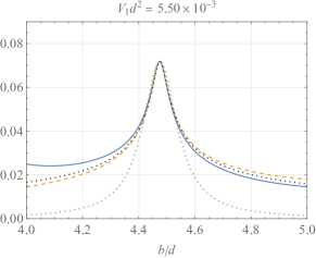
We find that when two QNM frequencies approach each other during the migration, they exhibit the same behavior observed for the Kerr QNMs; The two QNM frequencies repel each other, during which the excitation factors are point-symmetrically amplified. In the left and middle columns of Fig. 4, we depict the trajectories of QNM frequencies and excitation factors with respect to the variation of . In addition to , we control the second parameter to see how the avoided crossing and resonance change. The cases with and demonstrate sharp resonances, where the trajectories follow the hyperbola and lemniscate. The two cases switch about 90 degrees on the complex plane from each other, which is predicted at the sign flip of the RHS of in the main text. The cases with and show mild resonances. The trajectories of the QNM frequencies and excitation factors can be regarded as distorted versions of the hyperbola and lemniscate, respectively. These sharp and mild resonances reproduce what we observed in the Kerr QNM frequencies and excitation factors in the main text.
We also examine the characteristic resonant peak appearing in the difference of the excitation factors and the inverse of the difference of the QNM frequencies. As shown in the right column of Fig. 4, the peaks are well fitted by the quarter-power Lorentzian, same as the Kerr case. For the sharp resonances, the relative difference between any pair of , (normalized by multiplying a numerical constant), and the quarter-power Lorentzian remains % in the plotted region. The mild resonances are still better fitted by the quarter-power Lorentzian over the Lorentzian itself.
Note also that the resonance phenomenon occurs between the fundamental mode and third overtone of the first sequence. It implies that, while the resonances for Kerr QNMs studied in the main text occur for higher overtones, the resonances involving the fundamental mode and/or lower overtones are in general not prohibited. Indeed, we analyze the double rectangular barriers with various parameter sets and confirm the resonances for various pairs of two modes approaching each other. It suggests that the resonance is a universal feature of QNMs.