Neutrino-driven Core-collapse Supernova Yields in Galactic Chemical Evolution

Abstract

We provide yields from 189 neutrino-driven core-collapse supernova (CCSN) simulations covering zero-age main sequence masses between $11$ and $75\ \mathrm{M}_{\odot}$ and three different metallicities. Our CCSN simulations have two main advantages compared to previous methods used for applications in Galactic chemical evolution (GCE). Firstly, the mass cut between remnant and ejecta evolves naturally. Secondly, the neutrino luminosities and thus the electron fraction are not modified. Both is key to obtain an accurate nucleosynthesis. We follow the composition with an in-situ nuclear reaction network including the 16 most abundant isotopes and use the yields as input in a GCE model of the Milky Way. We adopt a GCE which takes into account infall of gas as well as nucleosynthesis from a large variety of stellar sources. The GCE model is calibrated to reproduce the main features of the solar vicinity. For the CCSN models, we use different calibrations and propagate the uncertainty. We find a big impact of the CCSN yields on our GCE predictions. We compare the abundance ratios of C, O, Ne, Mg, Si, S, Ar, Ca, Ti, and Cr with respect to Fe to an observational data set as homogeneous as possible. From this, we conclude that at least half of the massive stars have to explode to match the observed abundance ratios. If the explosions are too energetic, the high amount of iron will suppress the abundance ratios. With this, we demonstrate how GCE models can be used to constrain the evolution and deaths of massive stars.

1 Introduction

When massive stars explode as core-collapse supernovae (CCSNe) at the end of their evolution, they expel a significant fraction of their mass into the interstellar medium (ISM), including elements synthesized during hydrostatic burning phases as well as heavier elements beyond iron produced in explosive nucleosynthesis. As was shown by Romano et al. (2010), the amount and composition of the ejecta are a key uncertainty in models of Galactic chemical evolution (GCE) (see also Prantzos et al., 2018; Kobayashi et al., 2020; Palla et al., 2020). These models require a large grid of stellar progenitors, varying in mass and metallicity. However, even though the currently available yield grids come from updated stellar evolution and nucleosynthesis calculations, they can still significantly differ from each other. As a consequence, the same GCE models with the same assumptions on the main ingredients, produce different elemental abundances for different sets of yields. Although three-dimensional (3D) simulations are now accessible (see e.g. Janka et al., 2016; O’Connor & Couch, 2018; Ott et al., 2018; Burrows et al., 2020; Sandoval et al., 2021; Nakamura et al., 2022), simulating hundreds of CCSN models for several seconds is only feasible with one-dimensional (1D) simulations owing to computational cost. The stellar models that have been used so far for GCE have severe limitations related to the assumption of spherical symmetry. The multi-dimensional effects need to be replaced by an artificial energy source to trigger explosion. Previous massive star yields are usually obtained from semi-analytic prescriptions (Pignatari et al., 2016) or from simulations assuming spherical symmetry, where such an artificial energy source is added and the mass cut between the remnant and the ejecta is a free parameter (Umeda & Nomoto, 2005; Woosley & Heger, 2007; Limongi & Chieffi, 2018). In the present study, we multiply the neutrino energy deposition by a ’heating factor’. This method has the advantage that the mass cut evolves naturally in the simulations and that the neutrino luminosities are not modified. Our CCSN simulations include a state-of-the-art, two-moment neutrino treatment (Just et al., 2015), which takes all important neutrino interactions into account and allows for a self-consistent determination of the electron fraction in the ejecta. All approaches to explode massive stars in spherical symmetry have one or more free parameters (e.g. the amount of energy injected, where it is injected, the mass cut, the heating factor), which have to be calibrated to either more realistic 3D simulations or to properties of observed CCSNe. The choice of the calibration significantly impacts the final yields and can even decide between successful and failed explosion for the same stellar progenitor (see e.g. Young & Fryer, 2007; Couch et al., 2020). The question of explodability is a key problem in CCSN theory since it was found that there is no simple relation between the zero-age main sequence mass of a star and its final fate (see e.g. Ugliano et al., 2012; Sukhbold et al., 2016; Müller et al., 2016). There is no agreement between different studies on which stellar progenitors are expected to explode, although several criteria have been developed to enable this prediction (O’Connor & Ott, 2011; Ertl et al., 2016; Gogilashvili & Murphy, 2022; Boccioli et al., 2023). Additional uncertainties that enter in CCSN simulations are related to the adopted high-density equation of state (see e.g. Schneider et al., 2019; Yasin et al., 2020; Pascal et al., 2022), neutrino transport (see e.g. Iwakami et al., 2020; Wang & Burrows, 2023), pre-supernova stellar models (see e.g. Woosley et al., 2002; Ekström et al., 2012; Müller et al., 2017a; Cristini et al., 2017; Limongi & Chieffi, 2018; O’Connor & Couch, 2018; Fields & Couch, 2021; Yoshida et al., 2021; Vartanyan et al., 2022), the impact of magnetic fields and rotation (see e.g. Kuroda et al., 2020; Jardine et al., 2022; Obergaulinger & Aloy, 2022; Varma et al., 2022; Li et al., 2023), as well as the nucleosynthesis (see e.g. Harris et al., 2017; Navó et al., 2023; Sieverding et al., 2023). In this study, we use more than one calibration to account for this uncertainty and show how the uncertainty propagates into GCE models. Our aim is not to provide exact results, but to observe trends by including extreme scenarios of all stars exploding or only half of them.

Besides observations of the light curves and spectra of individual events, GCE models build the bridge to compare the yields predicted by CCSN simulations with the observed chemical properties of the ISM and stellar populations they ultimately try to reproduce. With the growing amount of observational data that is arriving from several Galactic archaeology surveys (e.g., the Galactic Archaeology with HERMES survey, GALAH, Buder et al., 2021; the Apache Point Observatory Galactic Evolution Experiment project, APOGEE, Majewski et al., 2017; the AMBRE project, de Laverny et al., 2013; the Gaia-ESO project, Mikolaitis et al., 2014), the need to build a self-consistent model of GCE able to provide stringent constraints on both stellar astrophysics and on the evolutionary history of our own Galaxy is becoming more and more important. Interpretation of observations from abundance surveys may be complex and, often, chemical evolution studies have to rely on a certain number of assumptions due to our limited understanding of some key parameters (e.g., star formation, initial mass function, gas flows and stellar migration). Nevertheless, GCE models have been proven to be powerful tools in investigating the production sources and timescales of different isotopes. To investigate the origin of the elements it is of great importance to build a self-consistent chain between stellar evolution, nucleosynthesis calculations and, finally, GCE models. In this study, we go all the way from simulating the collapse and explosion of massive stars, providing the nucleosynthesis results and using them as input for a GCE model to be able in the end to compare the results to observations of abundances for our own Galaxy.

The paper is structured as follows. In Section 2, we introduce the setup and input for our CCSN simulations, discuss the relation of progenitor properties and explosion dynamics, and explain how we obtain our massive star yields for GCE. In Section 3, we describe the adopted GCE and our main results for the solar abundances, the metallicity distribution function of the solar neighborhood and, finally, the abundance patterns of the elements produced by our new CCSN simulations. Section 4 summarises and discusses the results.

2 Core-collapse supernova yields

2.1 Hydrodynamic code

We have simulated 189 models of CCSNe with the magneto-hydrodynamics code Aenus-Alcar (Just et al., 2015; Obergaulinger & Aloy, 2022). The code includes special relativity, a pseudo-relativistic gravitational potential and a two-moment (M1) neutrino transport. The simulations employ spherical symmetry and a logarithmic grid with $1000\text{\,}$ cells in the radial direction and a central width of $200\text{\,}\mathrm{m}$. The simulations end after $1.5-5$ seconds once the yields have saturated. The SFHo nuclear equation of state (EOS) (Steiner et al., 2013) describes the matter at $T>$5.8\text{\,}\mathrm{GK}$$ assuming a nuclear statistical equilibrium (NSE) between protons, neutrons, alpha particles, and a representative heavy nucleus. Below this threshold NSE freezes out and the composition is obtained with a reduced nuclear reaction network (Navó et al., 2023) and an EOS taking into account photons, electrons, positrons and ions (Timmes & Arnett, 1999). In this work, we employ the 16-$\alpha$ chain reaction network, which has the smallest computational cost out of the implemented networks and gives comparable results to the larger networks in 1D simulations (for a comparison, see Navó et al., 2023). Between those regimes, the two EOS are interpolated linearly in order to prevent discontinuities in the thermodynamic quantities. The initial conditions for the reduced nuclear reaction network are given by an NSE solver considering the same nuclei as the network at $T=$5.8\text{\,}\mathrm{GK}$$.

2.2 Enhanced neutrino heating

It is a long-standing problem in CCSN simulations that only spherically symmetric models are feasible for systematic studies of large sets of initial conditions in terms of computational cost. The lack of multi-dimensional effects prevents these models from exploding self-consistently. There have been many approaches to artificially trigger explosions. Classic approaches are the so-called piston method (Woosley & Heger, 2007), where a mass element is followed along a ballistic trajectory or a kinetic bomb (Limongi & Chieffi, 2018), where kinetic energy is placed in a chosen mass shell. In the thermal bomb approach (Thielemann et al., 1996; Umeda & Nomoto, 2008; Imasheva et al., 2022), it is thermal energy that is injected. These methods are useful to obtain explosions and to investigate the dynamics and outcome of explosions of varying strength. However, the mass cut between the proto-neutron star (PNS) and the ejecta is a free parameter in these methods and its position significantly influences the ejecta mass and composition. In the neutrino light bulb method (Ugliano et al., 2012; Yamamoto et al., 2013), the PNS is replaced by inner boundary conditions. With this, the luminosity of neutrinos is a free parameter, the choice of which alters the electron fraction (due to neutrino reactions determining the proton to neutron ratio) and thus affects the nucleosynthesis. More recent approaches estimate the strength of convection and turbulence using a modified mixing length theory or enhance the neutrino energy deposition in the gain layer (e.g. STIR method: Couch et al., 2020 and PUSH method: Perego et al., 2015). The listed approaches differ in many ways, but they all have free parameters, which have to be calibrated to either observed supernova properties or to 3D simulations. We will show, in this work, that the results highly depend on the choice of this calibration and how this uncertainty propagates in subsequent applications.
In our artificial explosions, we enhance the neutrino heating in the gain layer by multiplying the energy source term $Q_{\text{E}}$, which describes the change of the energy density owing to neutrino reactions in the corresponding hydrodynamic equation, by a ’heating factor’. The heating factor (HF) is applied when two conditions are met: Firstly, the density is required to be below a threshold ($\rho<$1\text{\times}{10}^{10}\text{\,}\mathrm{g}\text{\,}{\mathrm{cm}}^{-3}$$) to confine the region to be outside the PNS. Secondly, there must be a positive energy gain from neutrino-matter interactions ($Q_{\text{E}}>0$) in the cell before adding the artificial heating. These conditions confine the area, where the HF is applied, to the gain region, so neutrino heating is enhanced while neutrino cooling is not modified. Since the energy increase via the HF is artificial, it is desirable to reduce it to the necessary minimum for a successful explosion. Therefore, the HF is applied only until the shock has reached a certain radius, after which it is unlikely to fall back onto the PNS. This radius is the second free parameter of our model. Once the shock reaches the chosen radius, the HF is set to one and has no further impact. It has been tested that this abrupt switch-off does not lead to instabilities in the hydrodynamic quantities and that a linear transition produces the exact same results. Note that our method shares with the PUSH and STIR methods the following advantages. Firstly, the PNS is included in the simulation domain and the mass cut evolves naturally in the simulation. Secondly, we only influence the total energy of the system, so the neutrino transport and thus the electron fraction are not modified. The nucleosynthesis in the innermost ejecta depends directly on the explosion dynamics, and specifically, on the electron fraction in these layers.

2.3 Stellar models

For a systematic study on the impact of the progenitor mass and structure on the explosion outcome, we run simulations with in total $63$ progenitor models of the non-rotating series of Woosley et al. (2002) (WHW02) with zero-age main sequence (ZAMS) masses of $11-30\ M_{\odot}$ in steps of $1\ M_{\odot}$ for three different metallicities, namely primordial, $10^{-4}$ solar, and solar metallicity. Additionally, we simulate the explosion of the solar metallicity models with ZAMS masses $35$, $40$, and $75\ M_{\odot}$. The progenitors with the same masses, but different metallicity likely form black holes, which cannot be captured in our simulations. Note that the stellar models with solar metallicity experience a significant amount of mass loss during their evolution and their mass will be much reduced at the time of the collapse, where our simulations begin (see Fig. 1). This is not the case for progenitors of primordial metallicity and also not for the intermediate metallicity of $10^{-4}$ solar. It is known that stars can be fast rotating and that this affects the structure and composition of the star (for a detailed discussion, see Limongi & Chieffi, 2018). Nevertheless, we do not include any rotating stars in this study. We denote the stellar models as ’mX’, where ’m’ indicates the metallicity (’s’ stands for solar metallicity, ’u’ for $10^{-4}$ solar, and ’z’ for primordial metallicity) and ’X’ is the ZAMS mass in solar masses. The simulations are denoted as ’mX-HF’, where the HF is added to the previous notation.
O’Connor & Ott (2011) define the compactness parameter

$$\xi_{\text{M}}=\frac{M/M_{\odot}}{R(M_{\text{bary}}=M)/$1000\text{\,}\mathrm{km}$}|_{t=t_{\text{bounce}}}$$ (1)

to link the progenitor structure to the explosion outcome in a simple way. They state that there is a threshold at which higher compactness always leads to black hole formation. The compactness is evaluated at the time of bounce as this is the most unambiguous point in core collapse. In Fig. 2, we display the compactness parameter evaluated for two mass shells for our set of progenitors. We come back to the relation of progenitor structure and its final fate in Section 2.4.

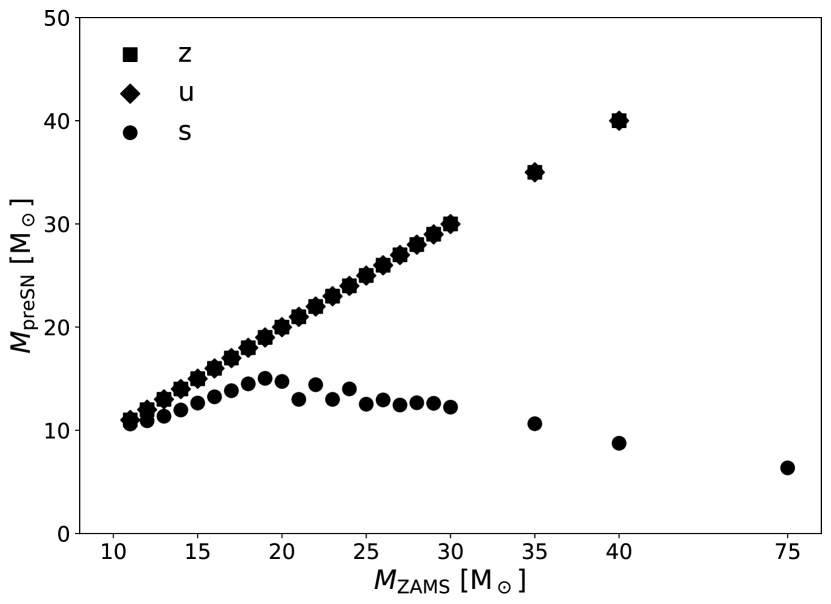
Figure 1: Progenitor mass at the onset of our simulations for all stellar models employed from the series of Woosley et al. (2002). The symbols indicate the initial metallicity.

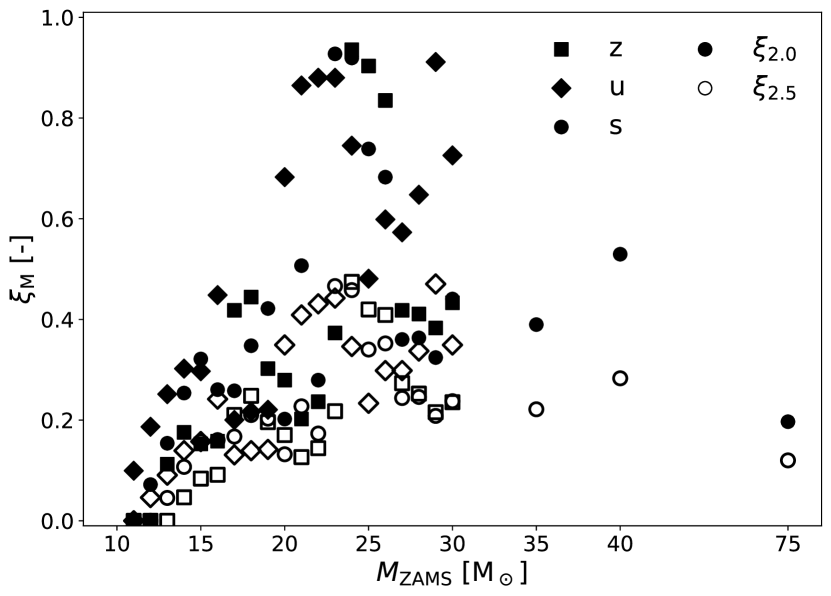
Figure 2: Compactness parameter for all progenitor models for mass shells $M=$2.0\text{\,}$M_{\odot}$ (filled circles) and $M=$2.5\text{\,}$M_{\odot}$ (open circles). If it is zero, less than $2\ M_{\odot}$ lie within the simulation region. The pattern is the same, but it is more pronounced for the mass shell enclosing $2\ M_{\odot}$. The symbols indicate the initial metallicity.

We employ several calibrations of our setup to estimate the uncertainty of our CCSN yields and propagate this uncertainty to the model of GCE. First, we calibrate to SN1987A, which is the most studied observed supernova event and has rather well constrained properties, in particular the explosion energy $E_{\text{exp}}=$1.1(3)\text{\,}\times\mathrm{1}\mathrm{0}^{51}\mathrm{e}\mathrm{r}\mathrm{g}$=$1.1(3)\text{\,}\mathrm{B}$$ (Blinnikov et al., 2000) and the amount of ejected Nickel $M(^{56}\text{Ni})=$0.071(3)\text{\,}$\ M_{\odot}$ (Seitenzahl et al., 2014). Four models of Woosley et al. (2002) have been used for the calibration: the solar metallicity models with ZAMS masses of $18\ M_{\odot}$, $18.8\ M_{\odot}$ and $19.8\ M_{\odot}$ as well as the primordial-metallicity model with a ZAMS mass of $18\ M_{\odot}$ (see Ugliano et al., 2012; Perego et al., 2015; Sukhbold et al., 2016; Ebinger et al., 2019; Curtis et al., 2018 for a similar calibration). For the sake of reaching the high explosion energy of the order of $1\text{\,}\mathrm{B}$, a very high HF of $5.6$, which is kept until the shock reaches $12\,000\text{\,}\mathrm{km}$, is needed for these progenitors. These values represent the upper limits for our free parameters. With this setup, all stellar models explode. On the lower end, we calibrate to a 3D simulation of the solar metallicity model with a ZAMS mass of $25\ M_{\odot}$ without rotation nor magnetic field, and without HF as this is not needed in 3D models. The simulation led to an explosion energy of $E_{\text{exp}}=$0.62\text{\,}\mathrm{B}$$, which can already be met with a HF of $2.4$, which is kept until the shock reaches $4000\text{\,}\mathrm{km}$. With these low values, only a fraction of about 40 per cent of our models explode. For stars that do not explode, all material falls back onto the remnant and no matter is ejected. We use these values as a lower limit. We find that for many models, the threshold of explodability lies in the region of the HF between $2.5$ and $2.7$ and decide to use $2.7$ as an intermediate and more standard case. Again, we keep the HF until the shock has reached $4000\text{\,}\mathrm{km}$. With this, we have nine failed explosions (about 14 per cent) in agreement with the inferred fraction of failed SNe of about 16 per cent (Neustadt et al., 2021).
In 1D simulations, the total energy of unbound material saturates or even decreases after a few hundred milliseconds. Since there is no simultaneous accretion and ejection in a spherically symmetric model, no more energy is injected into matter that is unbound. In multi-dimensional models, the explosion energy keeps rising for several seconds due to continuing accretion on the PNS (see e.g. Bruenn et al., 2016; Witt, 2020; Burrows et al., 2024). Since the explosion energy is expected to increase further for several seconds, we use the peak value of the total energy of unbound material (without overburden) as diagnostic explosion energy instead of the value at the last time step. One has to keep in mind the limitations of 1D simulations and that they are more suitable to observe trends rather than exact numbers. We take this into account by varying our free parameters and exploring a large range of possible explosion outcomes.

2.4 Explosion dynamics

We find a high dependency of the explosion outcome on the choice of the HF, even decisive about a successful explosion as it was explained in the previous Section. For many models, the threshold of explodability is around $\text{HF}=2.5-2.7$. In general, a higher HF adds more energy to the system, which results in earlier explosions of higher explosion energy. With the calibration that yields the highest explosion energies, all models explode and roughly at the same time around $0.2\text{\,}\mathrm{s}$ post-bounce. But there are exceptions to this trend, because the dynamics of the explosion mechanism highly depend on the stellar structure. A lower HF leads to later explosions, so that the layers behind the shock spend more time in the vicinity of the PNS, where they can gain most energy. Additionally, the increased accretion in these models powers stronger neutrino luminosities. This can, in some cases, lead to a higher explosion energy with a lower HF (e.g. models z25 and u29).

Many studies aimed to infer the explosion outcome from characteristics of the progenitor structure (see e.g. Sukhbold et al., 2016; Ertl et al., 2016; Müller et al., 2016; O’Connor & Ott, 2011; Ebinger et al., 2019). For some time, they have mostly reproduced the statement of O’Connor & Ott (2011) that a high compactness parameter has a tendency to correlate with black hole formation. Ebinger et al. (2019) adopted the assumption that progenitors with high compactness are unlikely to explode and calibrated the PUSH method in a compactness-dependent way, artificially reproducing this assumption. However, Couch et al. (2020) do not find that progenitors with a high compactness are particularly difficult to explode. They highlight that this is a distinguishing feature between the STIR method and the 1D neutrino-driven explosion model of Sukhbold et al. (2016) and Ertl et al. (2016). Note that Couch et al. (2020) use the same set of progenitors that was used in Sukhbold et al. (2016). They draw the conclusion that including the impact of turbulent convection in 1D simulations results in dynamics that are significantly different from those for purely neutrino-driven 1D explosions. Meanwhile, studies of multi-dimensional CCSN simulations have confirmed that stars with higher compactness are actually easier to explode. Vartanyan & Burrows (2023) have analysed 100 2D simulations and they state that models between $12$ and $15\ M_{\odot}$ are more difficult to explode, because they have shallow Silicon-Oxygen (Si/O) interfaces, whose accretion is not sufficient to revive the shock expansion. In many progenitors, the accretion of the Si/O-interface is accompanied with a sudden decrease in density and thus a drop in the accretion ram pressure, which can aid the initiation of the explosion (see Summa et al., 2016 and Boccioli et al., 2023 for more details on the role of the Si/O-interface). Burrows et al. (2024) have analysed a suite of twenty state-of-the-art 3D CCSN simulations. Only four of their simulations result in black hole formation and they state that the models with ZAMS masses $12.25$ and $14\ M_{\odot}$ have a too low compactness to explode.
The present approach, which is purely neutrino-driven and spherically symmetric, also readily explodes progenitors with high compactness, and even with less additional heating than progenitors with a small compactness parameter. Our explodability pattern aligns well with the findings of multi-dimensional simulations and STIR (see Fig. 3). Low compactness stars with $\xi_{2.0}<0.4$ fail to explode with the lowest HF. Around the threshold of $\xi_{2.0}=0.4$, there is no clear cut and stars with similar compactness can explode or not explode for the same HF, depending on their detailed structure. Above the threshold, the simulations result in explosion. The models that only explode with our highest HF mostly have ZAMS masses in the range of $11-15\ M_{\odot}$ (see zero iron ejection for non-exploding models in Fig. 4).
The compactness parameter does not only indicate whether a star is likely to explode, but is also connected to the explosion energy. Barker et al. (2022) employ the STIR method (Couch et al., 2020) and find a positive correlation between the compactness parameter of a progenitor and its explosion energy and explain this with the higher gravitational binding energy that is available in the explosion of models with more compact cores. Burrows et al. (2024) have confirmed this correlation with their suite of 3D simulations. Our simulations (though purely neutrino-driven and 1D) reproduce this correlation of explosion energy with progenitor compactness, independent of the choice of calibration (see Fig. 3).

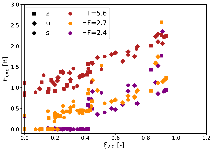
Figure 3: Relation of diagnostic explosion energy and compactness parameter $\xi_{2.0}$ for all models. If $\xi_{2.0}$ is zero, less than $2\ M_{\odot}$ lie within the simulation region. If $E_{\mathrm{exp}}$ is zero, the stellar model did not explode in our simulation. The different symbols indicate the initial metallicity, the colors the adopted heating factor.

2.5 Yields

From our simulations, we obtain the CCSN yields with a reduced, in-situ nuclear reaction network. We have compared the abundance pattern of the in-situ network with a full network calculation in post-processing using WinNet (Reichert et al., 2023) and we have found that the abundances of the main isotopes are well reproduced with the reduced network (Navó et al., 2023). Note that it is the shell just above the PNS that produces significant amounts of ⁴⁴Ti, ⁴⁸Cr, ⁵²Fe, ⁵⁴Fe, and mostly ⁵⁶Ni. Therefore, the exact location of the mass cut between the remnant and the ejecta determines the yields of a CCSN. Our simulations include the region of the PNS and do not require an assumption on the mass cut.
In Fig. 4, we present the amount of iron that is ejected in all our CCSN simulations. When the iron yield is zero, that means that the simulation did not result in an explosion and correspondingly, all yields are zero. The iron comes from the decay of radioactive ⁵⁶Ni. We find a correlation between the ejected amount of ⁵⁶Ni and the explosion energy that is independent on the metallicity or adopted heating factor (see Fig. 5). This is a well-known relation, which has been theoretically expected from semi-analytic CCSN models (e.g. Pejcha & Thompson, 2015) as well as from simulations (e.g. Sukhbold et al., 2016, Ebinger et al., 2019, Burrows et al., 2024) and has been observed astronomically (e.g. Hamuy, 2003, Müller et al., 2017b). Comparing more quantitatively to the 3D simulations by Burrows et al. (2024), our results agree in that simulations with explosion energies around $0.5-$1.25\text{\,}\mathrm{B}$$ eject around $0.1\ M_{\odot}$ of ⁵⁶Ni. For higher explosion energies, there is a better agreement with their results for our two lower heating factors. The amount of ⁵⁶Ni ejected by our simulations with $\text{HF}=5.6$ is much higher than what they find for explosion energies between $1.5-$2.5\text{\,}\mathrm{B}$$.

Figure 4: Iron ejected during the explosion (total, not net and no wind) for all models. The different symbols indicate the initial metallicity, the colors the adopted heating factor.

Figure 5: Relation of ejected iron and diagnostic explosion energy for all models. The different symbols indicate the initial metallicity, the colors the adopted heating factor.

In the following, we describe how we obtain the massive star yields from our CCSN simulations to apply them in our GCE model. In our GCE model, we take away the ZAMS mass of a star from the ISM when it is formed and give back the same initial mass with its initial composition to the ISM when the star dies. The stellar nucleosynthesis, both hydrostatic and explosive, is taken into account by adding net yields to the initial ones when they are given back.
We obtain the net yields in the following way. Material in cells that lie above the innermost cell with positive total energy density and that have positive radial velocity are considered to be unbound. For each of the 16 isotopes in our network, the mass of all unbound cells is summed up, once the yields have saturated (after $1$-$5\text{\,}\mathrm{s}$, depending on the model). We add, to the mass that is already unbound, all mass that is still outside the shock radius with the composition of the progenitor prior to the supernova simulation:

$$M_{\text{ejecta,i}}=M_{\text{unbound,i}}+M_{\text{envelope,i}}.$$ (2)

Most of these cells lie outside the simulation region. We expect that this mass would eventually be unbound with only minor changes in the composition if the simulation were to be continued to shock breakout. We consider all unstable isotopes to have decayed to stable isotopes. In GCE, we consider elements, not isotopes, so we sum together all isotopes of the same element. During their evolution of hydrostatic burning, the stars of solar metallicity will have ejected some of their mass in stellar winds. The mass of the wind can be obtained from the difference of the mass of the star prior to the supernova and in the ZAMS phase:

$$M_{\text{wind,i}}=X_{\text{wind,i}}\left(M_{\text{ZAMS}}-M_{\text{preSN}}\right).$$ (3)

The composition of the wind is not provided for the WHW02 progenitors. Compared to the explosive yields, the contribution from the wind to the final yields is negligible for all elements except for hydrogen and helium. We take the wind into account for mass conservation and assume a composition purely of hydrogen and helium. The ratio of those is inferred from wind data for a similar set of progenitors (Woosley & Heger, 2007). Only for the most massive progenitors ($30-75\ M_{\odot}$), this assumption underestimates the wind contribution for carbon and oxygen.
For the initial composition we multiply the expected mass fractions to the ZAMS mass of the model. For solar metallicity, we use the solar mass fractions of Anders & Grevesse (1989). For sub-solar metallicity, we rescale these mass fractions. For primordial metallicity, we assume the mass fractions $X=0.76$, $Y=0.24$, and $Z=0.00$ for H, He, and the other elements, respectively. The final net yields that are produced (or destroyed if negative) result in

$$M_{\text{final,i}}=M_{\text{ejecta,i}}+M_{\text{wind,i}}-M_{\text{ZAMS,i}}.$$ (4)

3 Galactic chemical evolution

In this Section, we present the chemical evolution models adopted in order to study the effect of the different massive star yields on the chemical evolution of the solar neighbourhood. In particular, the models are as follows:

• the one-infall model (see e.g., Matteucci & Greggio, 1986; Matteucci & Francois, 1989; Grisoni et al., 2018), according to which the solar vicinity forms by means of a single episode of primordial gas infall, with a timescale of $\mathrm{\tau\simeq 7\ Gyr}$.

• the delayed two-infall model of Spitoni et al. (2021) (see also Spitoni et al., 2019; Palla et al., 2020), which assumes that the Milky Way (MW) disc formed as a result of two different gas infall episodes. The delayed two-infall model is a variation of the classical two-infall model of Chiappini et al. (1997) (see also Chiappini et al., 2001) developed in order to fit the dichotomy in $\alpha$-element abundances observed both in the solar vicinity (e.g., Hayden et al., 2014; Recio-Blanco et al., 2014; Mikolaitis et al., 2017) and at various radii (e.g., Hayden et al., 2015). The model assumes that the first primordial gas infall event formed the chemically thick disc (namely the high-$\alpha$ sequence) whereas the second infall event, delayed by $\mathrm{\sim 4\ Gyr}$ formed the chemically thin disc (the low-$\alpha$ sequence). We stress that the two-infall model adopted here is not aiming to distinguish the thick and thin discs populations geometrically or kinematically (see Kawata & Chiappini, 2016 for a discussion).

The models are multi-zones, but here we focus on the evolution of the solar neighborhood only, corresponding to the Galactocentric distance $\mathrm{R_{GC}=8\ kpc}$. We adopt the metallicity dependent stellar lifetimes of Schaller et al. (1992) for stars with $\mathrm{0.1\leq M/M_{\odot}\leq 120}$.

3.1 The model

The basic equations which describe the evolution of the fraction of gas mass in the form of a generic chemical element $i$ are:

$$\dot{G}_{i}(R,t)=-\psi(R,t)X_{i}(R,t)+\dot{G}_{i,\text{inf}}(R,t)+R_{i}(R,t),$$ (5)

where $X_{i}(R,t)$ represents the abundance by mass of a given element $i$. $\psi(R,t)X_{i}(R,t)$ is the rate at which the element $i$ is subtracted from the ISM to be included in stars. $\psi(R,t)$ is the star formation rate (SFR), here parametrized according to the Schmidt-Kennicutt law (Kennicutt, 1998):

$$\psi(R,t)\propto\nu\sigma_{\text{gas}}(R,t)^{k},$$ (6)

with $k=1.5$ and $\sigma_{\text{gas}}$ being the surface gas density. The star formation efficiency, $\nu$, is a function of the Galactocentric distance, with $\mathrm{\nu(8\ kpc)=1\ \text{Gyr}^{-1}}$. $\dot{G}_{i,\text{inf}}(R,t)$ is the rate at which the element $i$ is accreted through infall of gas. For the two-infall model, the accretion term is computed as:

$$\dot{G}_{i,\text{inf}}(R,t)=AX_{i,\text{inf}}e^{-\frac{t}{\tau_{1}}}+\theta(t-t_{\text{max}})BX_{i,\text{inf}}e^{\frac{t-t_{\text{max}}}{\tau_{2}}},$$ (7)

where $X_{i,\text{inf}}$ is the composition of the infalling gas, here assumed to be primordial for both the infall events. $\tau_{1}\simeq 0.1\ \text{Gyr}$ and $\tau_{2}\simeq 4\ \text{Gyr}$ are the infall timescales for the first and the second accretion event, respectively, and $t_{\text{max}}\simeq 4\ \text{Gyr}$ is the time for the maximum infall on the disc and it corresponds to the start of the second infall episode. The parameters $A$ and $B$ are fixed to reproduce the surface mass density of the MW disc at the present time in the solar neighborhood. In case of single infall, the formulation for the accretion of gas is the following, simpler, one:

$$\dot{G}_{i,\text{inf}}(R,t)=BX_{i,\text{inf}}e^{-\frac{t}{\tau}}.$$ (8)

Different gas flows than the infall ones (Galactic winds and/or Galactic fountains) are not included. In particular, Galactic fountains, which are more likely to occur in disc galaxies, should not impact in a significant manner the chemical evolution of the disc (see e.g. Melioli et al., 2009).
Finally, $R_{i}(R,t)$ is the rate of restitution of matter from the stars with different masses into the ISM in the form of the element $i$. This last term takes into account a large variety of stars and phenomena, such as stellar winds, SN explosions of all types, novae and neutron-star mergers. It depends also on the initial mass function (IMF), which here is taken from Kroupa et al. (1993). In this work, we are interested in testing the yields prescriptions of CCSNe described in the previous Sections. Concerning the stellar yields of the other sources, for all stars sufficiently massive to die in a Hubble time, the following prescriptions have been adopted:

• for low-intermediate mass stars (LIMS, $\mathrm{1\leq M/M_{\odot}\leq 8}$), we adopt the non-rotational set of yields available on the F.R.U.I.T.Y. data base (Cristallo et al., 2009, 2011, 2015).

• for Type Ia SNe, we assume the single-degenerate scenario for the progenitors with stellar yields from Iwamoto et al. (1999) (their model W7).

• for nova systems we adopt prescriptions from José & Hernanz (2007).

• for neutron-star mergers, which do not affect significantly the elements treated in this paper but are important for the production of neutron-capture elements, we adopt the prescriptions described in Molero et al. (2023). Magneto-rotational SNe are also included in the model, but exclusively for the production of neutron-capture elements.

As described in Section 2.3, the yields adopted for massive stars are a grid of models in the mass range $\mathrm{11-75\ M_{\odot}}$ and initial metallicities $\mathrm{Z=0.0}$, $\mathrm{Z=10^{-4}\times Z_{\odot}}$ and $\mathrm{Z=Z_{\odot}}$. The adopted solar chemical composition is the one of Anders & Grevesse (1989), corresponding to $\mathrm{Z_{\odot}\simeq 0.02}$. For each metallicity, the models are computed for three different HFs: $\mathrm{2.4,2.7,5.6}$. The grid of yields corresponding to the progenitor mass range of $\mathrm{11-30\ M_{\odot}}$ is provided in steps of $\mathrm{1\ M_{\odot}}$ for the three metallicities and the three HFs, providing great precision in the computation of the chemical evolution. Grids of yields for the ZAMS stars with masses $\mathrm{35}$, $\mathrm{40}$, and $\mathrm{75\ M_{\odot}}$ are provided only for solar metallicity. For each HF, stars at solar metallicity that are not exploding are assumed to contribute to the chemical enrichment only through the wind. Because of the high precision in the progenitors stellar masses, the chemical evolution model does not require interpolation in large mass ranges for CCSN yields. On the other hand, the model interpolates in the mass range between super-AGB stars and low mass CCSNe (in this model this mass range is $\mathrm{8-11\ M_{\odot}}$, but it can vary depending on the adopted sets of yields from LIMS and massive stars), where no complete grid is currently available. In fact, the recently new set of yields from Limongi et al. (2024) for this mass range provides yields only at solar metallicity while for super and massive-AGB stars, yields from Doherty et al., 2014b, a are computed only until $\mathrm{9.0\ M_{\odot}}$. This interpolation can potentially be a source of uncertainty since, once weighted with the IMF, this mass range is one of the major contributors to the Galactic enrichment (see Romano et al., 2010 for a full discussion). Mass conservation is ensured, with massive star remnant (neutron star, black hole or white dwarf) masses being equal to the progenitor mass subtracted by the total ejected mass in the form of the different chemical species.

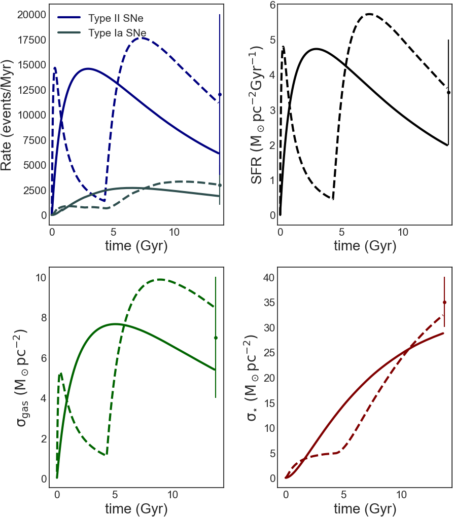
Figure 6: Time evolution of the rate of Type Ia SNe, Type II SNe (upper left panel), SFR (upper right panel), surface densities of gas (lower left panel) and of stars (lower right panel) as predicted by the one- (solid lines) and by the two-infall (dashed lines) models. Predictions of the models are compared to present day values from Cappellaro et al. (1999) (for SNe rates) and from Prantzos et al. (2018) (for SFR and surface gas and stars densities).

Comparisons of the evolution of some important quantities predicted by our model to present-day observations are reported in Fig. 6. The predicted SFR, and surface densities of stars and gas are computed in the solar neighbourhood and compared with present-day estimates as suggested by Prantzos et al. (2018). Rates of Type Ia and Type II SNe are averaged over the whole disc and compared with the observational estimates of Cappellaro et al. (1999). There is a satisfactory agreement with rates of all kinds of SNe as well as with the SFR, and surface densities of gas and stars. In general, the two-infall model provides the best agreement. One of the main observables in the solar neighbourhood is the metallicity distribution function (MDF) which will be discussed in the next Section, because of its dependence on the Fe yield and therefore on the CCSN prescriptions.

3.2 Results

In this Section, we present the results for the solar elemental abundances and MDF predicted by both the one- and the two-infall models. Then, we discuss, for each element, the behaviour of their abundance ratios as functions of metallicity in the typical $\mathrm{[X/Fe]}$ vs. $\mathrm{[Fe/H]}$ diagrams. We will refer to models with HF=2.4, 2.7, 5.6 as models M-24, M-27 and M-56, respectively. For comparison, we show also the results with the non-rotating massive star yields set of Limongi & Chieffi (2018). We will refer to this model as model M-LC. Because of the differences between our stellar and nucleosynthetic models with those of Limongi & Chieffi (2018), this comparison is intended to be only qualitative. All the other important parameters of the chemical evolution model, such as IMF, SFR, infall parameters, etc. are kept the same.

3.2.1 Solar abundances and metallicity distribution function

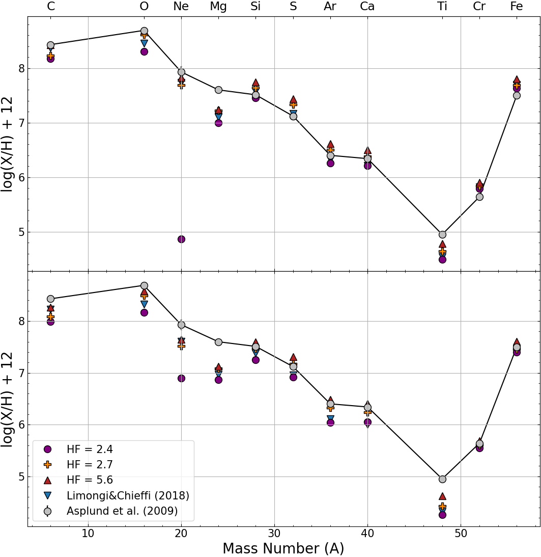
Figure 7: Predicted log(X/H)+12 solar abundances for Fe, C, O, Ne, Mg, Si, S, Ar, Ca, Ti and Cr obtained at the time of the formation of the Solar System by one- (upper panel) and two-infall (lower panel) models using different SNe Type II yield sets. The predictions are compared to the observed photospheric solar abundances by Asplund et al. (2009).

In Fig. 7, we show the solar abundances for Fe, C, O, Ne, Mg, Si, S, Ar, Ca, Ti and Cr predicted by the one- and the two-infall models, compared with the observed photospheric solar abundances by Asplund et al. (2009). At solar metallicity, the adoption of a larger HF increases considerably the production of all elements, not necessarily in a linear fashion. For the majority of the elements, the models which better agree with the observed solar abundances are model M-27 and M-56, with either $\mathrm{HF=2.7}$ or $\mathrm{HF=5.6}$. The best fit with the Fe abundance, in particular, is obtained for the two-infall model with $\mathrm{HF=2.7}$. Similar results are obtained by adopting the yields from Limongi & Chieffi (2018), which here have been used as a second, theoretical, comparison. In particular, since our new CCSN models do not include rotation, we are using the Limongi & Chieffi (2018)’s yields set R with no initial rotational velocity. However, we remind the reader that the inclusion of rotation in stellar evolutionary models (and as a consequence in chemical evolution studies as well) significantly alters the outputs of traditional nucleosynthesis, increasing the yields of almost all elements by factors which depend on the metallicity (we refer to Cescutti et al., 2013; Prantzos et al., 2018; Romano et al., 2019; Rizzuti et al., 2019; Molero et al., 2024 for more discussions on the effect of massive stellar rotators to the chemical evolution of different nuclear species). The majority of the solar abundances for elements studied here are reproduced to more than 95 per cent by the two-infall model with higher HF, with the exception of Ne which is underproduced in almost all models and the usual exceptions of Mg and Ti, which are underproduced. The problem of the Mg and Ti underproduction is present in the majority of massive stars yield sets, including Woosley & Weaver (1995); François et al. (2004); Limongi & Chieffi (2018) and it will be discussed further in Section 3.2.2.

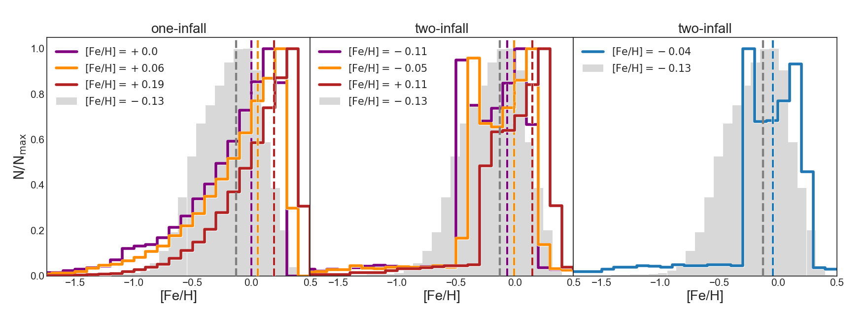
Figure 8: MDF in the solar neighborhood predicted by the one- (left panel) and the two- (middle and right panels) infall models for the three different HFs ($\mathrm{HF=2.4}$ purple line; $\mathrm{HF=2.7}$ orange line; $\mathrm{HF=5.6}$ red line) and for the Limongi & Chieffi (2018)’s yields (blue line) compared with data from the SDSS/APOGEE DR17 sample (grey region). In the legends are reported the predicted and observed values of the median of the distributions.

In Fig. 8, we present our results for the solar neighbourhood MDF predicted by the one- and the two-infall models for the different sets of yields adopted. The predicted MDFs are compared with data from the SDSS/APOGEE DR17 sample of stars with Galactocentric distance $\mathrm{7\leq R_{GC}\leq 9\ kpc}$. The observed MDF is characterized by a single-peak shape, with the peak position at $\mathrm{[Fe/H]\simeq 0.0\ dex}$ and a median at $\mathrm{[Fe/H]=-0.13\ dex}$. The single-peak shape is nicely obtained also by our one-infall model, for each value of the HF. The one-infall model results tend, however, to overestimate the number of stars both in low-metallicity ($\mathrm{[Fe/H]\leq-0.75\ dex}$) and in the high-metallicity ($\mathrm{[Fe/H]\geq-0.25\ dex}$) regions, with this latter in a more severe manner. Increasing the HF increases the production of Fe and, as a consequence, causes a shift in the MDF towards higher metallicity. This effect is reduced with the two-infall model, for which the predicted MDFs remain confined in the observed metallicity range even for larger HFs. For $\mathrm{HF=5.6}$, the model still overestimates the number of stars at high [Fe/H], but in a less dramatic way with respect to the correspondent one-infall model. Moreover, for all the HFs, the two-infall models do not overestimate stars in the low-metallicity regime. In the case of the non-rotational set of yields from Limongi & Chieffi (2018), the two-infall models do not show particular differences. By looking at the overall MDF shape and at the predicted median values (see legends in Fig. 8), the models that agree better with the observed MDF, are the two-infall models with low to intermediate HFs (models M-24 and M-27). The MDF shape has a strong dependence on the stellar yields because of the different Fe production. However, it must be reminded that to properly constrain the model with the MDF, dynamical features such as stellar migration and radial gas flows should be taken into account (see e.g., Minchev et al., 2013; Spitoni et al., 2015; Grisoni et al., 2018; Palla et al., 2020; Vincenzo & Kobayashi, 2020). Nevertheless, since this work is restricted to the study of the impact of new yield sets on the chemical evolution, it most probably benefits the most in the framework of a simpler GCE model. Therefore, as a first approach, dynamical effects on stars and gas have been excluded.

3.2.2 Abundance ratios

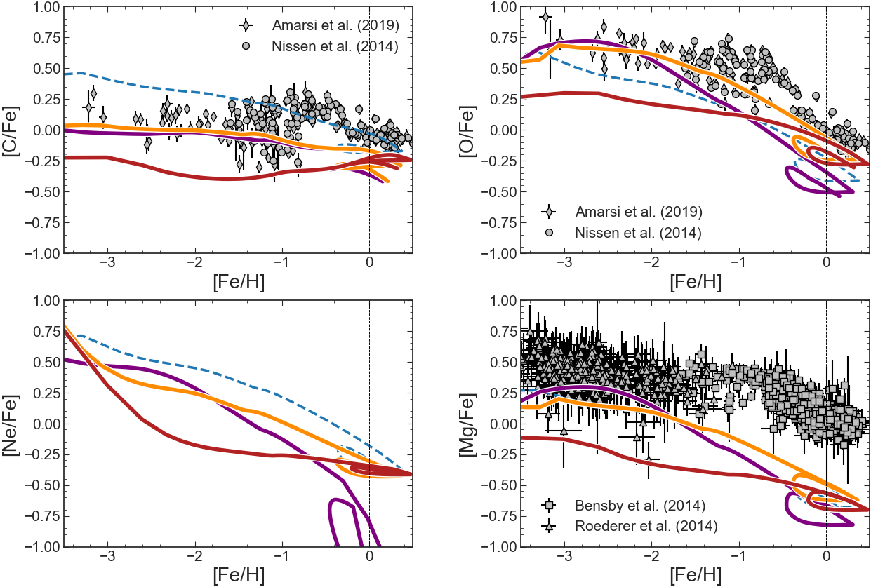
(a)

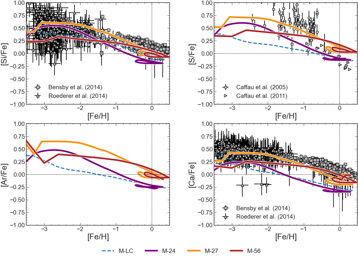
(b)

Figure 9: Evolution of abundance ratios [X/Fe] vs. [Fe/H] for C, O, Ne, Mg, Si, S, Ar and Ca compared to observational data. Model M-24, M-27 and M-56 include the new sets of yields with HFs $\mathrm{HF=2.4,2.7}$ and $\mathrm{5.6}$, respectively. Model M-LC correspond to the non-rotational yield set R from Limongi & Chieffi (2018)

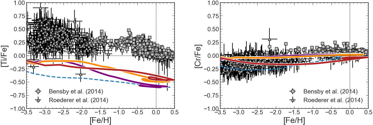
Figure 10: Same as Fig. 9 but for Ti and Cr.

In this Section, we present the predicted behaviour of the different abundance ratios as a function of metallicity for the elements produced by the CCSN models. We use Fe as a metallicity indicator and show the results in the typical [X/Fe] vs. [Fe/H] diagnostic diagrams. We will show results only for the two-infall models, which, with the current set of yields, agrees better with the solar abundances as well as with the MDF, as shown in the previous Section. Results are displayed in Figures 9 and 10. We compare our model results with data from only a few surveys, to keep the data set as homogeneous as possible and to not overcrowd the plots. Nevertheless, some dispersion in the data is still visible at low metallicity probably due to the inhomogeneities in the ISM (see e.g., Cescutti, 2008 and Cescutti & Chiappini, 2014).

Carbon: For the analysis of the [C/Fe] vs. [Fe/H] trend, we adopt data from Nissen et al. (2014) and Amarsi et al. (2019) (grey circles and diamonds in Fig. 9, respectively). Note that this is the same observational set adopted by Romano et al. (2019), where the evolution of the CNO isotopes is widely investigated (see also Romano & Matteucci, 2003; Romano et al., 2017). Nissen et al. (2014) determined abundances for C, O and Fe for F and G main-sequence stars in the solar vicinity with $\mathrm{-1.6<[Fe/H]<+0.4\ dex}$. Carbon abundances are determined from the $\lambda\lambda 5052,5380\ \rm{CI}$ lines to which 1D non-local thermodynamic equilibrium (non-LTE) corrections were applied. The observed stars belong to different stellar populations, including both thin and thick discs as well as the halo. Amarsi et al. (2019) carried out 3D non-LTE radiative transfer calculations for $\rm CI$ and $\rm OI$. The derived absolute corrections between the 3D non-LTE and 1D LTE were used in the re-analysis of C, O and Fe in F and G dwarfs belonging to the MW disc and halo with $\mathrm{[Fe/H]\leq-1.5\ dex}$. The behaviour of [C/Fe] at low metallicities observed in the data from Amarsi et al. (2019) is rather flat, with almost a solar value. This flat trend is nicely reproduced by models M-24 and M-27 that assume low HFs (2.4 and 2.7). The two models predict similar results for all the range of metallicity, with model M-27 only slightly above model M-24. The increase of the HF to the high value of $\mathrm{HF=5.6}$ does not translate into a higher [C/Fe] trend. Since, after weighting by the IMF, the Fe enrichment is greater than the C one, the line corresponding to model M-56 lies below those of models M-24 and M-27 for all the range of metallicity, reaching similar values only at solar. The $\mathrm{[C/Fe]\sim 0}$ produced by model M-24 and M-27 is obtained also with the yields from Woosley & Weaver (1995) and from Nomoto et al. (2013) (without hypernovae). Data with $\mathrm{[Fe/H]\geq-1.6}$ from Nissen et al. (2014) are not reproduced by the models with our new sets of yields, which underestimate the [C/Fe] ratio. On the other hand, model M-LC provides an adequate fit to this observed trend, but it fails to reproduce the flat trend at low [Fe/H].

$\alpha$-elements: For the $\alpha$-elements O, Si, S, and Ca, we adopt different sets of observational data from Caffau et al. (2005, 2011); Nissen et al. (2014); Bensby et al. (2014); Roederer et al. (2014) and Amarsi et al. (2019). Bensby et al. (2014) conducted a high-resolution spectroscopic study of F-G dwarf and subgiant stars in the solar neighborhood. In particular, they selected stars kinematically belonging to the thin and thick discs, the metal-rich halo as well as to sub-structures as the Hercules stream and the Arcturus moving group. The elemental abundances have been determined using 1D, plane-parallel model atmospheres under the LTE assumption, correcting the $\rm{FeI}$ lines for non-LTE effects. The low metallicity data are from Roederer et al. (2014). The authors presented detailed abundances from high resolution optical spectroscopy of 313 metal-poor stars. They performed a standard LTE abundance analysis by using 1D model atmospheres for their analysis, applying line-by-line statistical corrections. The observational data adopted for the [S/Fe] vs. [Fe/H] are from Caffau et al. (2005) and Caffau et al. (2011). Caffau et al. (2005) assembles a sample of 253 stars with metallicity in the range $\mathrm{-3.2\leq[Fe/H]\leq+0.5\ dex}$ made of both literature data and their own measurements of 74 Galactic stars high resolution spectra. From their sample a significant scatter in the [S/Fe] at $\mathrm{[Fe/H]\simeq-1.0\ dex}$ is observed, that the authors did not attribute necessarily to distinct stellar populations. As shown in Fig. 9, data are showing the typical abundance pattern of $\alpha$-elements, characterized by a plateau and by a high [$\alpha$/Fe] ratio at low [Fe/H] values, where the production of both $\alpha$-elements and Fe is only due to CCSNe, and a decrease in [$\alpha$/Fe] ratio with higher [Fe/H] because of the late injection of Fe from Type Ia SNe (time-delay model, Matteucci, 2012). Model M-24, with the lowest HF, tends to underestimate the observed abundance pattern of all $\alpha$-elements and for almost all the range of metallicity. In fact, for $\mathrm{HF=2.4}$, only few progenitors are actually exploding at primordial and solar metallicity. The majority of them are exploding at intermediate metallicity, causing the peak in the [$\alpha$/Fe] at $\mathrm{[Fe/H]\simeq-3\ dex}$. After the peak, the model quickly decreases with metallicity because of the strong contribution to the Fe production by Type Ia SNe, which is not being compensated by CCSNe. As a consequence, model M-24 cannot reproduce the typical ’plateau’ like pattern of $\alpha$-elements, and, except at $\mathrm{[Fe/H]\leq-2\ dex}$ for O and Si, it underestimates the general trend for the entire range of metallicity. Increasing the HF to the high value of $\mathrm{HF=5.6}$ allow us to obtain results in agreement with the typical ’plateau’ like trend but, because of the stronger production of Fe than $\alpha$-elements, the model lies under the observed trend for all the range of metallicity, similarly to what happens with C. The underproduction is not critical in the case of Si, S and Ca, in particular at intermediate and at solar metallicity. In fact, even though the predicted trend is generally below the observed one, some stars have abundances that may be consistent with a stronger explosion, similarly to what has been found by Romano et al. (2010) in the case of hypernovae. Model M-27, with an intermediate value for the HF, produces the best agreement with the observations for all the $\alpha$-elements, in particular below $\mathrm{[Fe/H]\simeq-1.0\ dex}$. Towards higher [Fe/H], the model tends to slightly underestimate the observed trend, as in the case of O and Ca. However, since this discrepancy is present in a metallicity range where the contribution to the Fe (and partially also to $\alpha$-elements) from Type Ia SNe is not negligible, it is difficult to state to what extend this inconsistency is due to CCSNe only.

Magnesium and Titanium: Concerning Mg and Ti, their evolution is not well reproduced by our model. The solar abundance of these two elements is underestimated, as explained above, and the underproduction characterizes their whole evolution. Only model M-24 provide a slight agreement with the data from Roederer et al. (2014) for the [Mg/Fe] at low [Fe/H] values, but it is considered by no means to be satisfactory. Depending on the model, [Mg/Fe] and [Ti/Fe] are $\sim 0.25-0.4\ \mathrm{dex}$ underabundant overall. The underproduction of Mg and Ti is a well known problem in GCE. Similar results to those obtained here arise also with yields of different authors (as for example those of Woosley & Weaver, 1995 and of Limongi & Chieffi, 2018 for which we refer to the corresponding chemical evolution studies of Timmes et al., 1995 and Prantzos et al., 2018, respectively), which often need to be increased by large factors (see e.g. François et al., 2004). An alternative solution for Mg can be represented by the inclusion of hypernovae in the chemical evolution calculations, as shown by Kobayashi et al. (2006) and by Romano et al. (2010). In both cases, $\sim 50$ per cent of stars more massive than $20\ M_{\odot}$ should explode as hypernovae (this fraction can slightly change depending on the adopted IMF). On the other hand, up to date, no solution is known to correct the Ti abundances (see however Maeda & Nomoto, 2003). We remind the reader that this is not related to the problem of producing sufficient ⁴⁴Ti in CCSNe as this radioactive isotope decays to ⁴⁴Ca, while our Ti comes from the decay of ⁴⁸Cr.

Noble gases: We report the evolution also of the noble gases Ne and Ar for which, however, there are no observations in stars. Ne and Ar are $\alpha$-elements with plateau values predicted by our models of $\mathrm{[Ar-Ne/Fe]\sim 0.5\ dex}$ for $\mathrm{[Fe/H]\leq-1.0\ dex}$. Indeed, increasing the HF produces similar effects in Ne and Ar as in the other $\alpha$-elements. With respect to model M-LC, with Limongi & Chieffi (2018)’s yields, our models tend to underestimate and overestimate the [Ne/Fe] and [Ar/Fe] vs. [Fe/H] trends overall, respectively, independently on the HF.

Chromium: Model M-24 and M-27 produce near-solar [Cr/Fe] for all the range of metallicities, with a slightly decreasing trend toward lower [Fe/H]. This is well in agreement with observations which down to $\mathrm{[Fe/H]\sim-1.5\ dex}$ show a constant [Cr/Fe] ratio which then slightly decreases with decreasing metallicity. Since Cr, together with the other Fe-peak elements, is half produced by Type Ia SNe, which contribution is not a function of the metallicity, the increase of the [Cr/Fe] with [Fe/H] obtained by our model is only due to massive stars. Model M-56, tends to underestimate the overall trend, in particular at intermediate [Fe/H], most probably due to the stronger Fe production.

4 Conclusions

In this work, we provide a new set of CCSN yields and test them in a consistent model of GCE able to reproduce the main features of the Milky Way disc and of the solar vicinity. The new grid of stellar yields covers the mass range $\mathrm{11-75\ M_{\odot}}$, mostly in steps of $\mathrm{1\ M_{\odot}}$, and the initial metallicities $\mathrm{Z=0.0,10^{-4},1.0\ Z_{\odot}}$. In our spherically symmetric, neutrino-driven CCSN simulations, additional energy is injected with a ’heating factor’ (HF) to mimic the support to the neutrino heating mechanism by convection and turbulence. We test the impact of different calibration methods for these artificial explosions and find that the results significantly change when calibrating to SN1987A or to a 3D simulation. This uncertainty estimate is propagated by using three sets of yields with different HFs (2.4, 2.7, and 5.6) in our GCE model. The uncertainty in the CCSN yields is still relevant after weighting by the IMF and combining with other stellar sources. All predictions from our GCE model differ significantly for our three sets of yields. Generally, a higher HF increases the production of all elements. Interestingly, this does not result in linear trends in the abundance ratios.
The model that best reproduces the observations is the one with $\text{HF}=2.7$. It has the best agreement with the shape of the solar MDF, as well as the solar iron abundance, in particular in the case of a two-infall scenario of disc formation. This model also nicely reproduces the order of magnitude of the $\alpha$-elements abundance ratios as well as the trend with metallicity. The [Mg/Fe] and [Ti/Fe] vs. [Fe/H] abundance trends are underproduced with a slight improvement with respect to the non-rotational set of Limongi & Chieffi (2018). The evolution of [Cr/Fe] with [Fe/H] as well as the plateau observed in the [C/Fe] at low [Fe/H] is well reproduced by both models with lower HF.
Comparing the sets with $\text{HF}=2.4$ and $\text{HF}=2.7$, the main difference is that only about half of the stars explode with the lower HF. The question of the explodability pattern (which stars explode and how many of them) remains open. Our simulations, though 1D, reproduce the explodability pattern of recent 3D simulations. How many and which stars explode significantly changes the final yield predictions, because for a star that does not explode, the CCSN contribution is lost. Since the set with the lowest HF underproduces almost all elements, this suggests that at least half of the massive stars have to explode to fit the observed chemical evolution of the solar neighbourhood.
We find a positive correlation between the amount of iron that is ejected and the explosion energy. This has been found in previous studies and shows that the dynamics of the explosions have a direct impact on the nucleosynthesis. Also the yields of the other elements are increased with higher explosion energy, but they do not scale as strongly. This is the main reason for the differences between the models with $\text{HF}=2.7$ and $5.6$. Most models explode in both cases, but, in general, the explosions with the higher HF are more energetic. The increased iron production reduces the ratio with respect to iron ([X/Fe]) for all elements and thus their abundance patterns seem to be underproduced. As a result, increased explosion energies of about $1-$2.5\text{\,}\mathrm{B}$$ lessen the agreement with the observational data. This indicates that the typical CCSN explosion energy should be lower than about $2\text{\,}\mathrm{B}$.
With this work, we proved the great importance of building a self-consistent chain between the final stage of stellar evolution, nucleosynthesis calculations and GCE models. We conclude that using late advances in spherically symmetric CCSN simulations or even the growing set of multi-dimensional simulations to obtain yields for GCE models can provide useful constraints to both fields.

Data Availability

The data underlying this article will be uploaded as extra material available online.

References

- Amarsi et al. (2019) Amarsi A. M., Nissen P. E., Skúladóttir Á., 2019, A&A, 630, A104
- Anders & Grevesse (1989) Anders E., Grevesse N., 1989, Geochim. Cosmochim. Acta, 53, 197
- Asplund et al. (2009) Asplund M., Grevesse N., Sauval A. J., Scott P., 2009, ARA&A, 47, 481
- Barker et al. (2022) Barker B. L., Harris C. E., Warren M. L., O’Connor E. P., Couch S. M., 2022, ApJ, 934, 67
- Bensby et al. (2014) Bensby T., Feltzing S., Oey M. S., 2014, A&A, 562, A71
- Blinnikov et al. (2000) Blinnikov S., Lundqvist P., Bartunov O., Nomoto K., Iwamoto K., 2000, ApJ, 532, 1132
- Boccioli et al. (2023) Boccioli L., Roberti L., Limongi M., Mathews G. J., Chieffi A., 2023, Astrophys. J., 949, 17
- Bruenn et al. (2016) Bruenn S. W., et al., 2016, ApJ, 818, 123
- Buder et al. (2021) Buder S., et al., 2021, MNRAS, 506, 150
- Burrows et al. (2020) Burrows A., Radice D., Vartanyan D., Nagakura H., Skinner M. A., Dolence J. C., 2020, MNRAS, 491, 2715
- Burrows et al. (2024) Burrows A., Wang T., Vartanyan D., 2024, preprint (arXiv:2401.06840)
- Caffau et al. (2005) Caffau E., Bonifacio P., Faraggiana R., François P., Gratton R. G., Barbieri M., 2005, A&A, 441, 533
- Caffau et al. (2011) Caffau E., Bonifacio P., Faraggiana R., Steffen M., 2011, A&A, 532, A98
- Cappellaro et al. (1999) Cappellaro E., Evans R., Turatto M., 1999, A&A, 351, 459
- Cescutti (2008) Cescutti G., 2008, A&A, 481, 691
- Cescutti & Chiappini (2014) Cescutti G., Chiappini C., 2014, A&A, 565, A51
- Cescutti et al. (2013) Cescutti G., Chiappini C., Hirschi R., Meynet G., Frischknecht U., 2013, A&A, 553, A51
- Chiappini et al. (1997) Chiappini C., Matteucci F., Gratton R., 1997, ApJ, 477, 765
- Chiappini et al. (2001) Chiappini C., Matteucci F., Romano D., 2001, ApJ, 554, 1044
- Couch et al. (2020) Couch S. M., Warren M. L., O’Connor E. P., 2020, ApJ, 890, 127
- Cristallo et al. (2009) Cristallo S., Straniero O., Gallino R., Piersanti L., Domínguez I., Lederer M. T., 2009, ApJ, 696, 797
- Cristallo et al. (2011) Cristallo S., et al., 2011, ApJS, 197, 17
- Cristallo et al. (2015) Cristallo S., Straniero O., Piersanti L., Gobrecht D., 2015, ApJS, 219, 40
- Cristini et al. (2017) Cristini A., Meakin C., Hirschi R., Arnett D., Georgy C., Viallet M., Walkington I., 2017, MNRAS, 471, 279
- Curtis et al. (2018) Curtis S., Ebinger K., Fröhlich C., Hempel M., Perego A., Liebendörfer M., Thielemann F.-K., 2018, ApJ, 870, 2
- Doherty et al. (2014a) Doherty C. L., Gil-Pons P., Lau H. H. B., Lattanzio J. C., Siess L., 2014a, MNRAS, 437, 195
- Doherty et al. (2014b) Doherty C. L., Gil-Pons P., Lau H. H. B., Lattanzio J. C., Siess L., Campbell S. W., 2014b, MNRAS, 441, 582
- Ebinger et al. (2019) Ebinger K., Curtis S., Fröhlich C., Hempel M., Perego A., Liebendörfer M., Thielemann F.-K., 2019, ApJ, 870, 1
- Ekström et al. (2012) Ekström S., et al., 2012, A&A, 537, A146
- Ertl et al. (2016) Ertl T., Janka H.-T., Woosley S. E., Sukhbold T., Ugliano M., 2016, ApJ, 818, 124
- Fields & Couch (2021) Fields C. E., Couch S. M., 2021, ApJ, 921, 28
- François et al. (2004) François P., Matteucci F., Cayrel R., Spite M., Spite F., Chiappini C., 2004, A&A, 421, 613
- Gogilashvili & Murphy (2022) Gogilashvili M., Murphy J. W., 2022, MNRAS, 515, 1610
- Grisoni et al. (2018) Grisoni V., Spitoni E., Matteucci F., 2018, MNRAS, 481, 2570
- Hamuy (2003) Hamuy M., 2003, Astrophys. J., 582, 905
- Harris et al. (2017) Harris J. A., Hix W. R., Chertkow M. A., Lee C. T., Lentz E. J., Messer O. E. B., 2017, Astrophys. J., 843, 2
- Hayden et al. (2014) Hayden M. R., et al., 2014, AJ, 147, 116
- Hayden et al. (2015) Hayden M. R., et al., 2015, ApJ, 808, 132
- Imasheva et al. (2022) Imasheva L., Janka H.-T., Weiss A., 2022, MNRAS, 518, 1818
- Iwakami et al. (2020) Iwakami W., Okawa H., Nagakura H., Harada A., Furusawa S., Sumiyoshi K., Matsufuru H., Yamada S., 2020, ApJ, 903, 82
- Iwamoto et al. (1999) Iwamoto K., Brachwitz F., Nomoto K., Kishimoto N., Umeda H., Hix W. R., Thielemann F.-K., 1999, ApJS, 125, 439
- Janka et al. (2016) Janka H.-T., Melson T., Summa A., 2016, Annu. Rev. Nucl. Part. Sci., 66, 341
- Jardine et al. (2022) Jardine R., Powell J., Müller B., 2022, MNRAS, 510, 5535
- José & Hernanz (2007) José J., Hernanz M., 2007, Journal of Physics G Nuclear Physics, 34, R431
- Just et al. (2015) Just O., Obergaulinger M., Janka H.-T., 2015, MNRAS, 453, 3387
- Kawata & Chiappini (2016) Kawata D., Chiappini C., 2016, Astronomische Nachrichten, 337, 976
- Kennicutt (1998) Kennicutt Robert C. J., 1998, ApJ, 498, 541
- Kobayashi et al. (2006) Kobayashi C., Umeda H., Nomoto K., Tominaga N., Ohkubo T., 2006, ApJ, 653, 1145
- Kobayashi et al. (2020) Kobayashi C., Karakas A. I., Lugaro M., 2020, ApJ, 900, 179
- Kroupa et al. (1993) Kroupa P., Tout C. A., Gilmore G., 1993, MNRAS, 262, 545
- Kuroda et al. (2020) Kuroda T., Arcones A., Takiwaki T., Kotake K., 2020, ApJ, 896, 102
- Li et al. (2023) Li L., Zhu C., Guo S., Liu H., Lü G., 2023, ApJ, 952, 79
- Limongi & Chieffi (2018) Limongi M., Chieffi A., 2018, ApJS, 237, 13
- Limongi et al. (2024) Limongi M., Roberti L., Chieffi A., Nomoto K., 2024, ApJS, 270, 29
- Maeda & Nomoto (2003) Maeda K., Nomoto K., 2003, ApJ, 598, 1163
- Majewski et al. (2017) Majewski S. R., et al., 2017, AJ, 154, 94
- Matteucci (2012) Matteucci F., 2012, Chemical Evolution of Galaxies. Springer-Verlag, Berlin
- Matteucci & Francois (1989) Matteucci F., Francois P., 1989, MNRAS, 239, 885
- Matteucci & Greggio (1986) Matteucci F., Greggio L., 1986, A&A, 154, 279
- Melioli et al. (2009) Melioli C., Brighenti F., D’Ercole A., de Gouveia Dal Pino E. M., 2009, MNRAS, 399, 1089
- Mikolaitis et al. (2014) Mikolaitis Š., et al., 2014, A&A, 572, A33
- Mikolaitis et al. (2017) Mikolaitis Š., de Laverny P., Recio-Blanco A., Hill V., Worley C. C., de Pascale M., 2017, A&A, 600, A22
- Minchev et al. (2013) Minchev I., Chiappini C., Martig M., 2013, A&A, 558, A9
- Molero et al. (2023) Molero M., Magrini L., Matteucci F., Romano D., Palla M., Cescutti G., Vázquez C. V., Spitoni E., 2023, MNRAS, 523, 2974
- Molero et al. (2024) Molero M., Matteucci F., Spitoni E., Rojas-Arriagada A., Rich R. M., 2024, preprint (arXiv:2405.12585)
- Müller et al. (2016) Müller B., Heger A., Liptai D., Cameron J. B., 2016, MNRAS, 460, 742
- Müller et al. (2017a) Müller B., Melson T., Heger A., Janka H.-T., 2017a, MNRAS, 472, 491
- Müller et al. (2017b) Müller T., Prieto J. L., Pejcha O., Clocchiatti A., 2017b, Astrophys. J., 841, 127
- Nakamura et al. (2022) Nakamura K., Takiwaki T., Kotake K., 2022, MNRAS, 514, 3941
- Navó et al. (2023) Navó G., Reichert M., Obergaulinger M., Arcones A., 2023, ApJ, 951, 112
- Neustadt et al. (2021) Neustadt J. M. M., Kochanek C. S., Stanek K. Z., Basinger C., Jayasinghe T., Garling C. T., Adams S. M., Gerke J., 2021, Mon. Not. Roy. Astron. Soc., 508, 516
- Nissen et al. (2014) Nissen P. E., Chen Y. Q., Carigi L., Schuster W. J., Zhao G., 2014, A&A, 568, A25
- Nomoto et al. (2013) Nomoto K., Kobayashi C., Tominaga N., 2013, ARA&A, 51, 457
- O’Connor & Ott (2011) O’Connor E., Ott C. D., 2011, ApJ, 730, 70
- Obergaulinger & Aloy (2022) Obergaulinger M., Aloy M. A., 2022, MNRAS, 512, 2489
- Ott et al. (2018) Ott C. D., Roberts L. F., Da Silva Schneider A., Fedrow J. M., Haas R., Schnetter E., 2018, ApJ, 855, L3
- O’Connor & Couch (2018) O’Connor E. P., Couch S. M., 2018, ApJ, 865, 81
- Palla et al. (2020) Palla M., Matteucci F., Spitoni E., Vincenzo F., Grisoni V., 2020, MNRAS, 498, 1710
- Pascal et al. (2022) Pascal A., Novak J., Oertel M., 2022, MNRAS, 511, 356
- Pejcha & Thompson (2015) Pejcha O., Thompson T. A., 2015, Astrophys. J., 801, 90
- Perego et al. (2015) Perego A., Hempel M., Fröhlich C., Ebinger K., Eichler M., Casanova J., Liebendörfer M., Thielemann F.-K., 2015, ApJ, 806, 275
- Pignatari et al. (2016) Pignatari M., et al., 2016, ApJS, 225, 24
- Prantzos et al. (2018) Prantzos N., Abia C., Limongi M., Chieffi A., Cristallo S., 2018, MNRAS, 476, 3432
- Recio-Blanco et al. (2014) Recio-Blanco A., et al., 2014, A&A, 567, A5
- Reichert et al. (2023) Reichert M., et al., 2023, ApJS, 268, 66
- Rizzuti et al. (2019) Rizzuti F., Cescutti G., Matteucci F., Chieffi A., Hirschi R., Limongi M., 2019, MNRAS, 489, 5244
- Roederer et al. (2014) Roederer I. U., Preston G. W., Thompson I. B., Shectman S. A., Sneden C., 2014, ApJ, 784, 158
- Romano & Matteucci (2003) Romano D., Matteucci F., 2003, MNRAS, 342, 185
- Romano et al. (2010) Romano D., Karakas A. I., Tosi M., Matteucci F., 2010, A&A, 522, A32
- Romano et al. (2017) Romano D., Matteucci F., Zhang Z. Y., Papadopoulos P. P., Ivison R. J., 2017, MNRAS, 470, 401
- Romano et al. (2019) Romano D., Matteucci F., Zhang Z.-Y., Ivison R. J., Ventura P., 2019, MNRAS, 490, 2838
- Sandoval et al. (2021) Sandoval M. A., Hix W. R., Messer O. E. B., Lentz E. J., Harris J. A., 2021, ApJ, 921, 113
- Schaller et al. (1992) Schaller G., Schaerer D., Meynet G., Maeder A., 1992, A&AS, 96, 269
- Schneider et al. (2019) Schneider A. S., Roberts L. F., Ott C. D., O’Connor E., 2019, Phys. Rev. C, 100, 055802
- Seitenzahl et al. (2014) Seitenzahl I. R., Timmes F. X., Magkotsios G., 2014, ApJ, 792, 10
- Sieverding et al. (2023) Sieverding A., Waldrop P. G., Harris J. A., Hix W. R., Lentz E. J., Bruenn S. W., Messer O. E. B., 2023, ApJ, 950, 34
- Spitoni et al. (2015) Spitoni E., Romano D., Matteucci F., Ciotti L., 2015, ApJ, 802, 129
- Spitoni et al. (2019) Spitoni E., Silva Aguirre V., Matteucci F., Calura F., Grisoni V., 2019, A&A, 623, A60
- Spitoni et al. (2021) Spitoni E., et al., 2021, A&A, 647, A73
- Steiner et al. (2013) Steiner A., Hempel M., Fischer T., 2013, ApJ, 774, 17
- Sukhbold et al. (2016) Sukhbold T., Ertl T., Woosley S. E., Brown J. M., Janka H.-T., 2016, ApJ, 821, 38
- Summa et al. (2016) Summa A., Hanke F., Janka H.-T., Melson T., Marek A., Müller B., 2016, ApJ, 825, 6
- Thielemann et al. (1996) Thielemann F.-K., Nomoto K., Hashimoto M.-A., 1996, ApJ, 460, 408
- Timmes & Arnett (1999) Timmes F. X., Arnett D., 1999, ApJS, 125, 277
- Timmes et al. (1995) Timmes F. X., Woosley S. E., Weaver T. A., 1995, ApJS, 98, 617
- Ugliano et al. (2012) Ugliano M., Janka H.-T., Marek A., Arcones A., 2012, ApJ, 757, 69
- Umeda & Nomoto (2005) Umeda H., Nomoto K., 2005, ApJ, 619, 427
- Umeda & Nomoto (2008) Umeda H., Nomoto K., 2008, ApJ, 673, 1014
- Varma et al. (2022) Varma V., Müller B., Schneider F. R. N., 2022, MNRAS, 518, 3622
- Vartanyan & Burrows (2023) Vartanyan D., Burrows A., 2023, MNRAS, 526, 5900
- Vartanyan et al. (2022) Vartanyan D., Coleman M. S. B., Burrows A., 2022, MNRAS, 510, 4689
- Vincenzo & Kobayashi (2020) Vincenzo F., Kobayashi C., 2020, MNRAS, 496, 80
- Wang & Burrows (2023) Wang T., Burrows A., 2023, ApJ, 943, 78
- Witt (2020) Witt M. R., 2020, Phd thesis, Technische Universität Darmstadt, http://tuprints.ulb.tu-darmstadt.de/11567/
- Woosley & Heger (2007) Woosley S. E., Heger A., 2007, Phys. Rep., 442, 269
- Woosley & Weaver (1995) Woosley S. E., Weaver T. A., 1995, ApJS, 101, 181
- Woosley et al. (2002) Woosley S. E., Heger A., Weaver T. A., 2002, Rev. Mod. Phys., 74, 1015
- Yamamoto et al. (2013) Yamamoto Y., Fujimoto S.-i., Nagakura H., Yamada S., 2013, ApJ, 771, 27
- Yasin et al. (2020) Yasin H., Schäfer S., Arcones A., Schwenk A., 2020, Phys. Rev. Lett., 124, 092701
- Yoshida et al. (2021) Yoshida T., Takiwaki T., Kotake K., Takahashi K., Nakamura K., Umeda H., 2021, ApJ, 908, 44
- Young & Fryer (2007) Young P. A., Fryer C. L., 2007, ApJ, 664, 1033
- de Laverny et al. (2013) de Laverny P., Recio-Blanco A., Worley C. C., De Pascale M., Hill V., Bijaoui A., 2013, The Messenger, 153, 18